1. Introduction

Ice cores contain a wealth of palaeoclimatic information (e.g. Reference LangwayLangway, 1967), but the ice temperature measured in the borehole itself can also reveal information about past climate. Atmospheric temperature acts as an upper boundary condition for the temperature within the ice sheet. This temperature signal is advected downwards and diffuses over time. At the bottom of an ice sheet the geothermal heat flux serves as a lower boundary condition for the internal temperature distribution. Ice flow may complicate the thermal profile as a result of horizontal and vertical advection, strain heating and friction near the bottom.

Several studies have been carried out to retrieve the temperature history at the surface from ice-temperature measurements along ice cores or in deep boreholes in polar areas (e.g. Dahl-Jensen andJohnsen, 1986; Reference Cuffey, Clow, Alley, Stuiver, Waddington and SaltusCuffey and others, 1995; Reference Dahl-JensenDahl-Jensen and others, 1998). Most of these studies focus on the temperature reconstruction on the glacial–interglacial time-scale because the cores come from ice sheets with large ice thickness and small accumulation rate. Although Reference Cuffey, Alley, Grootes, Bolzan and AnandakrishnanCuffey and others (1994) and Reference Dahl-JensenDahl-Jensen and others (1998) have also derived climate information over the last century from deep boreholes, the temperature reconstruction from medium-depth boreholes reported by Reference PatersonPaterson and Clarke (1978) on Devon Island, Canada, and Reference Nicholls and ParenNicholls and Paren (1993) on the Antarctic Peninsula has a greater similarity to the work presented in this study.

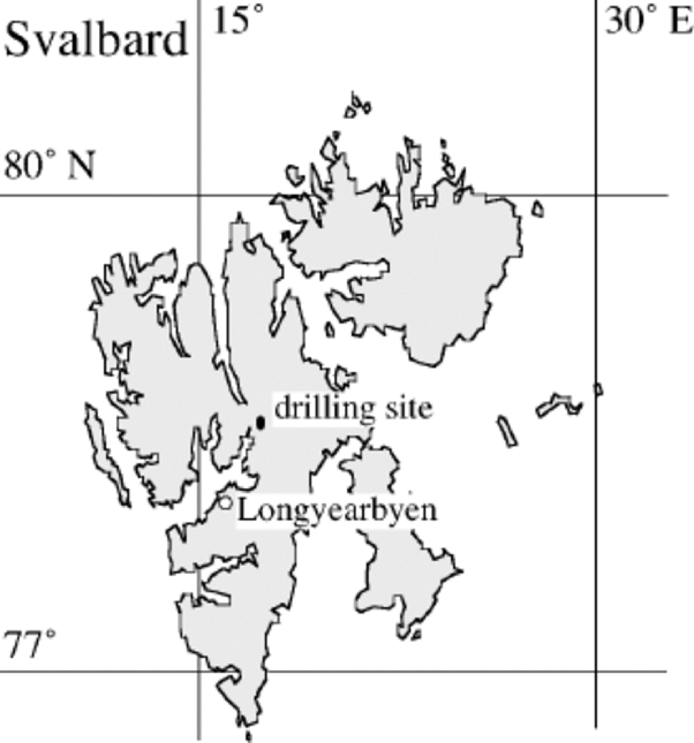
Here we consider the temperature profile in a medium-lengthborehole120mdeep drilled at the highest point of the Lomonosovfonna plateau, Svalbard (Fig. 1). Lomonosovfonna is one of the highest icefields in Svalbard and is a suitable site for retrieving ice cores. In April 1997 a 120 m deep ice core was drilled at the ice divide at 1230 ma.s.l. (78˚51’53’’N, 17˚25’30’’ E) by a Dutch–Norwegian–British– Swedish–Finnish team. the ice-core analysis programme includes measurements of dielectric and electrical properties, ice structures, β -activity, oxygen isotopes, deuterium, major ions and methanesulphonate. the influence of melt on the climatological signals in the ice core is discussed by Reference PohjolaPohjola and others (2002). Interpretation of the chemistry of the upper part of the core covering the period 1920–97 is presented by Reference IsakssonIsaksson and others (2001), while Reference O’DwyerO’Dwyer and others (2000) discuss the possibility of methanesulphonic acidmeasured in this core as an indicator of ocean climate.

Fig. 1

The Lomonosovfonna drilling site at 1230 m a.s.l.

The local ice thickness was measured using a Ramac ground-penetrating radar that generates a monopulse wavelet with a centre frequency of 50 MHz (Malå Geoscience, Sweden). Radar measurements were taken at approximately 2 m intervals on profiles to the west, south and east of the borehole, with five closest approaches to within 20m of the borehole, and radar travel time corresponding to 119–121m of solid ice. Correction for the lower-density firn was made from detailed density measurements performed on the upper 18m of core, which corresponds roughly to the firn/ice transition depth, to give a total ice thickness of 126.5±1.5 m.

The ¹³⁷Cs activity from the atmospheric thermonuclear tests was measured by high-resolution γ-spectrometry. the peak level corresponds to the 1963 level; using the integrated density measurements above this level reveals an accumulation rate of 380 kg m^–2 a^–1. Measurements by Reference Gordienko, Kotlyakov, Punning and VaikmyaeGordienko and others (1980), carried out ~250m lower and ~5 km downstream at the same glacier, indicate an accumulation rate of 820 kg m^–2 a^–1 over the period 1951–76. There is no sound explanation for the difference. This shallow ice thickness and accumulation rate imply that only a limited time range is covered by this core. Application of a Nye time-scale (Reference Paterson and ClarkePaterson 1994) indicates that the ice at 120m depth is approximately 1000 years old. This means that possible temperature changes during the 20th century can be detected. Verification of the estimated depth–age relation could provide better insight into the vertical velocity profile, but is beyond the scope of this paper.

In this paper we try to reconstruct the temperature history by solving the heat-flow equation for an ice divide numerically, neglecting the horizontal advection. We present the measurements in section 2, and briefly discuss the theory in section 3. In section 4 we discuss time-dependent solutions and a historical simulation. the role of refreezing is considered in the final section.

2. Measurements

Temperature was measured in the 120m deep borehole at the end of drilling by taking resistance measurements using a Fluke 8060A meter (characterized by a low current excitation to reduce self-heating) on three calibrated Betatherm Corporation type .3K3A1 thermistors (nominally 300 Ω at 25˚C) spaced 2 m apart on a four-core cable. the cable was lowered in 4m steps to overlap the upper and lower thermistors on each measurement cycle. Readings were taken several times at each depth to ensure the resistance had stabilized at the new temperature. Cable resistance was measured and subtracted from the thermistor resistances.

The thermistors were calibrated in the Cambridge laboratory in a cooled water bath, with salt added to depress the freezing point to –12˚C (personal communication from K. Makinson, 1997). Calibration data are taken at several points in the range –12˚ to + 15˚C against the water-bath temperature measured using an Automatic Systems Laboratories Ltd F300 Mk2 thermometry bridge and a Tinsley Model 5187SA Primary Standard Platinum Resistance Thermometer (SPRT), with a nominal resistance of 25 ±0.5Ω at 0.0000˚C. All temperatures use the reference T90 temperature scale, and the SPRT is regularly calibrated using the following fixed points:

In addition, the thermometer was calibrated commercially at the National Physics Laboratory against a lower fixed temperature:

Combining the calibrations of the thermometry bridge and SPRT, the calibration system has an accuracy of ±0.001˚C and resolution of 0.0001˚C.

With this level of calibration the thermistors should be accurate to 0.01±0.005K. However, we found that the uppermost thermistor gave results 0.1K higher than the other two thermistors; we assume that this thermistor had been damaged and the data were rejected. Ideally, measurements should be made several days after drilling, to allow the borehole temperature to relax after the drilling operation, but this was not possible due to lack of time in the field. One set of measurements over the depth range 0–82m was made within hours of completion of drilling, while a second set was made 16 hours later over the range 68–121m. Examination of the overlapping sections indicates the change in borehole temperature over the 16 hours was <0.01K, suggesting the measurements were not unduly affected by the drilling operation (which had taken 4 days to reach 120 m), but some noise is evident in the lowest readings, so we conservatively estimate the accuracy of our results to be no better than ±0.05K.

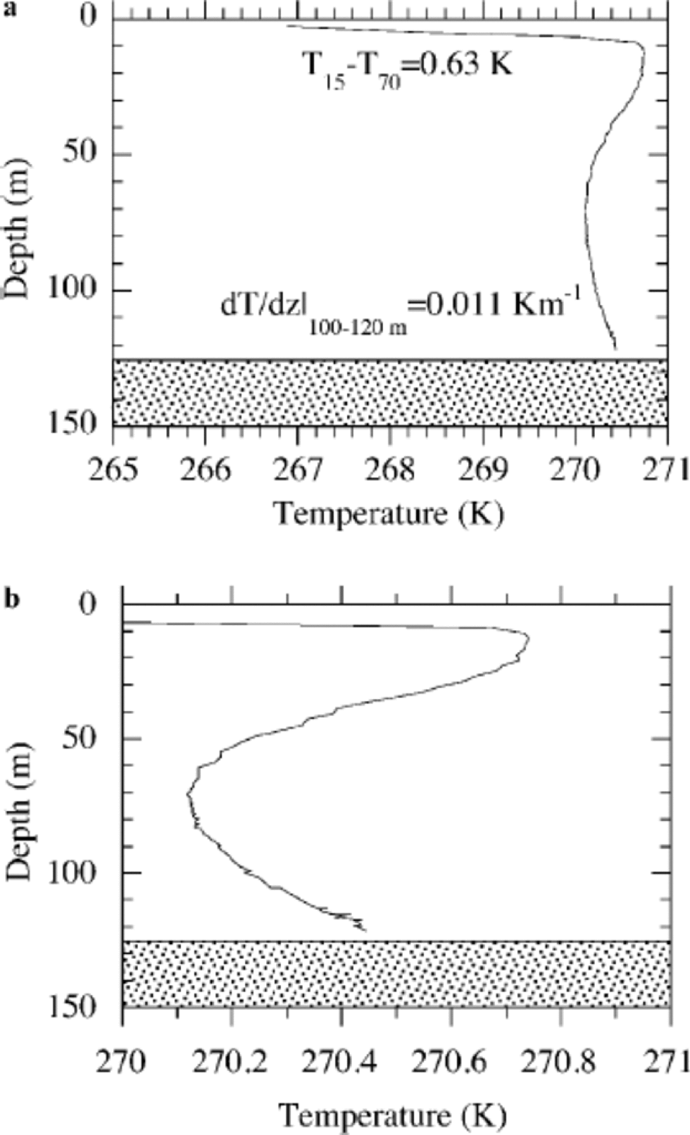
The temperature profile contains two striking features. Firstly, one observes that the profile is nearly isothermal but with a minimum at 70 m depth. Similar reverse temperature gradients are observed for some other ice cores on Svalbard (e.g. Reference Zagorodnov, Zotikov., Avsyuk and BalkemaZagorodnov and Zotikov, 1988, at the divide between eastern Grönfjordbreen and Fridtjovbreen; Reference UchidaUchida and others, 1996, at Åsgårdfonna). the observed temperature range at 15– 120m depth is only 0.6 K. Secondly, one observes that the gradient near the bottom is about 0.011Km^–1 in the section from 100 to 120m. This indicates a low value for the geothermal heat flux, since a typical geothermal heat flux of 50 mWm^–2 would yield a gradient of 0.02 Km^–1 under steady-state conditions (which do not necessarily apply as will be seen later). These two characteristics will be used at a later stage.

Note that a bottom temperature of approximately 270.5 K implies a permafrost layer of 100–350m, depending on the thermal conductivity of the rock. This is within the range observed on Svalbard (personal communication from J.O. Hagen, 1997). However, the permafrost thickness does not influence the ice-temperature calculations since the lower boundary condition is prescribed in terms of a temperature gradient, as discussed in the next section.

3. Theory

If we consider the thermodynamic equation where heat transfer is balanced by vertical conduction and vertical advection due to ice motion, we can write:

In this equation k is the thermal diffusivity and w is the vertical velocity. the vertical coordinate ranges from z = h at the surface to z =0 at the bottom and is positive upwards. Advection in the horizontal direction is neglected as we consider an ice divide. Since the measurements indicate basal temperatures below zero, friction at the bottom can also be neglected. A simple scale analysis, as described by Reference Cuffey, Alley, Grootes, Bolzan and AnandakrishnanCuffey and others (1994), shows that heat production to strain heating can be neglected.

The simplest solution for this equation is the steady-state solution with ∂T/∂t=0 We furthermore assume that k is independent of the temperature; this assumption is justified because of the nearly isothermal profile which leads to variations in k smaller than 1% of the mean value. Finally we have to assume that the glacier itself is in balance since a changing ice flow would change the vertical velocity profile and thus the advection and temperature profile.

In order to obtain a steady-state solution we impose the following boundary conditions for Equation (1): T = T_s at z = h – 15 m (temperature at 15 m depth which is a depth considered to be unaffected by the seasonal cycle), and dT/dz is constant at z = 0 (bottom). Integration of Equation (1) (with ∂T/∂t = 0) yields:

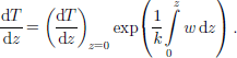
This can be solved analytically for certain functions of z. Three solutions will be considered in this analysis. We know w at the surface from the net accumulation rate, and w at the bottom must be zero. the simplest solution is w = –bz/h, where b is the net accumulation rate. the second solution, w = bz²/h², is more appropriate for an ice divide and has –been suggested by Reference RaymondRaymond (1983). the third solution assumes sliding and no deformation, implying that w is everywhere equal to the surface value. the last solution should be considered as a sensitivity test of the influence of the vertical velocity profile on the vertical temperature distribution.

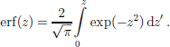
Integration of Equation (2) with a linear profile for w yields the Robin solution (Reference Robin and deRobin,1955) for steady state:

with l² = 2kh/b (b positive), and

4. Time-Dependent Solutions

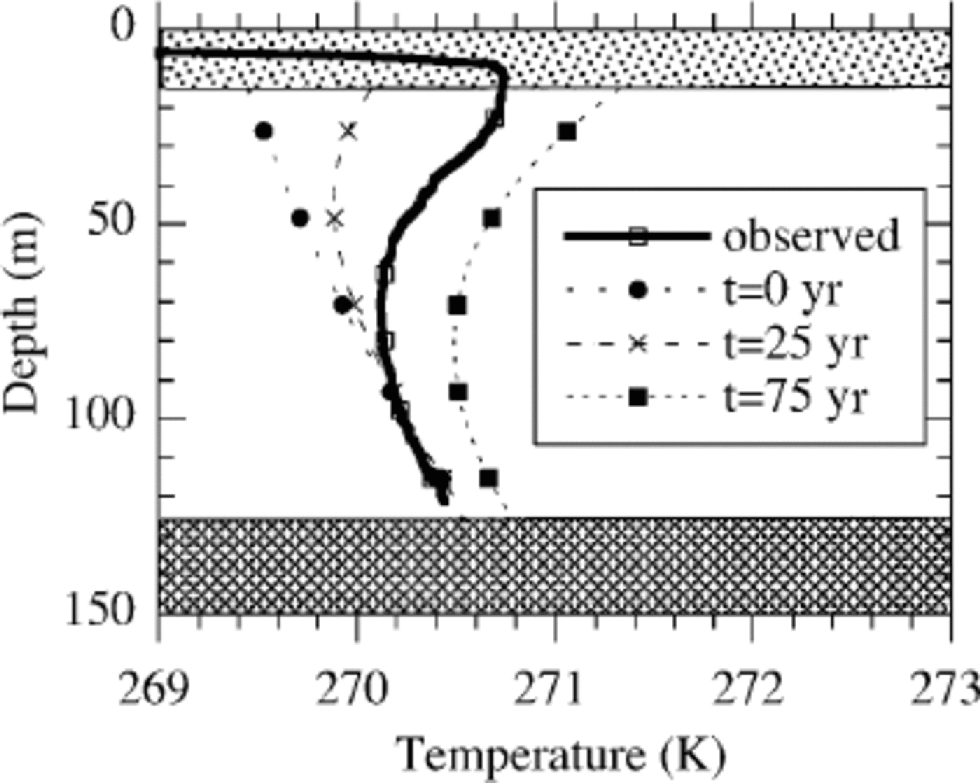
In Figure 2a we observe a significant decrease in temperature 15–70m below the surface; this cannot be attributed to a steady-state solution or uncertainty in the calculations. Therefore, we consider a non-steady state with the following parameter setting: H = 126.5 m, G = 25 mWm^–2, w_s = –0.38m a^–1, linear profile. for this purpose, Equation (1) has to be solved numerically (see Appendix). the vertical temperature profile is in principle determined by the temperature history, changes in ice thickness and changing geothermal heat flux. We consider cases where variations in ice thickness and geothermal heat flux can be neglected and are decoupled from variations in the temperature history. Given the limited constraints, we only consider solutions with a linear trend in temperature. to resolve the trend in the temperature we simply prescribe the temperature at 15 m depth (T^s) linearly in time (t):

Fig. 2

(a)Measurements of the temperature in the borehole; (b) same data but on a stretched horizontal scale.

At time t₀ the temperature at depth z =15m equals T₀ and the vertical profile is in steady state. In other words, if t < t₀ then T_s = T₀. Note that we introduce three parameters to be optimized (T₀, α, t). the reason for choosing this simple approach is the uniform temperature gradient at 15 –70 m, which suggests a simple form of temperature forcing. In practice, only a few attempts are needed to find the best solution for the rate of increase (α) and time (t), since the thermal inertia leads to a temperature minimum which travels downwards with a wave velocity that depends on the perturbation.

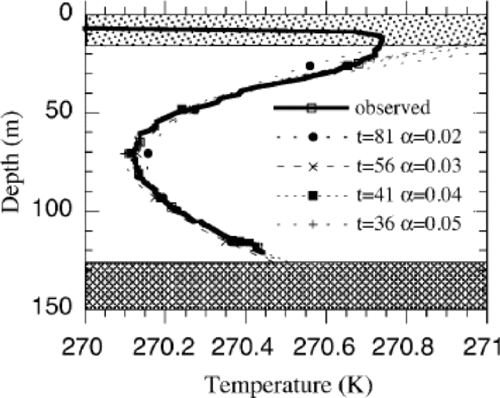
Figure 3 shows an example of the development of a temperature minimum and the downward migration of this minimum. There are three parameters, initial temperature, forcing rate and time, which are coupled, leading to unique solutions for the temperature distribution. Changing only one parameter will change the match between observations and calculations. the best solution is found after 56 years for a temperature increase of 0.03Ka^–1 (see Fig. 5). Increasing or decreasing the rate of the temperature change and simultaneously changing T₀ and t does not improve the match between observed and calculated temperature (see Fig. 4). Increasing the rate of temperature increase at the surface leads to an overestimation of the surface temperature, and decreasing the rate of increase leads to an overestimation of the temperature minimum. This means that we have at least one satisfactory temperature history which explains the upper half of the temperature profile.

Fig. 3

Temperature evolution in time for α = 0.03 Ka^–1. the initial profile and temperature profiles after 25 and 50 years are shown. the thick line represents the observations. the initial profile is determined by the observations near the bottom. Parameters: H = 126.5m, G = 25m Wm^–2, w_s = –0.38ma^–1, linear profile.

Fig. 4

Temperature profiles for different values of α (Ka^–1), showing the snapshots in time which resulted in the best match between observation and calculation for a particular value of α. Parameters: H =126.5, G = 25 m Wm^–w_s = -0.38 m a^–linear profile.

So far, we have considered a solution obtained from an initial equilibrium state at t₀. the limitation of this solution is that we have to use rather a low value for the geothermal heat flux in order to obtain a reasonable match between the observed temperature gradient and the calculated one near the bottom. Physically there is of course no reason to assume that the initial state is in equilibrium. the observed low gradient near the bottom actually points to a non-steady state, even near the bottom of the core.

Figure 5 illustrates the evolution of the gradient between 100 and 120m in a 126.5m deep borehole in the case of two different perturbations. the geothermal heat flux is 37.5m Wm^–2 in these calculations. This means that at t₀ the gradient is 0.02Km^–1 in this depth interval under steady-state conditions. the observed gradient was 0.011Km^–1. If the boundary condition at the surface is changed, the temperature profile has to adjust in time with this forcing. Diffusion and advection will slowly change the temperature from the top to the bottom. As a direct result, the gradient near the bottom will decrease (see Fig 6). One observes that soon after the perturbation at the surface has terminated, the temperature gradient near the bottom increases again. the initial steady-state gradient will be reached after about 500 years. the typical response time (1 – 1e–²) before the temperature gradient is close to the equilibrium value again is about 228 years (which is independent of the magnitude of the temperature increase).

Fig. 5

The evolution of the temperature gradient near the bottom of the core in the case of an increase of 0.02 and 0.04 Ka^–1 over a period of a 100 years (indicated by the vertical line). the horizontal line indicates the observed gradient in this section. Parameters: H = 126.5m, G = 37.5 m Wm^–2, w_s = –0.38 m a^–1, linear profile.

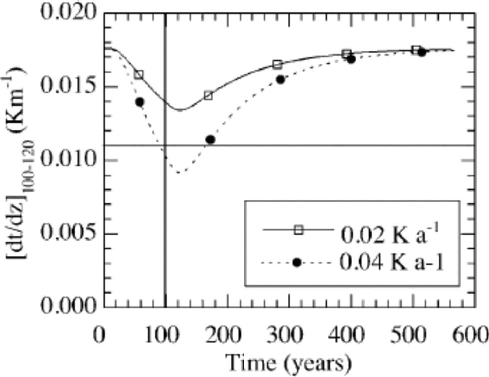
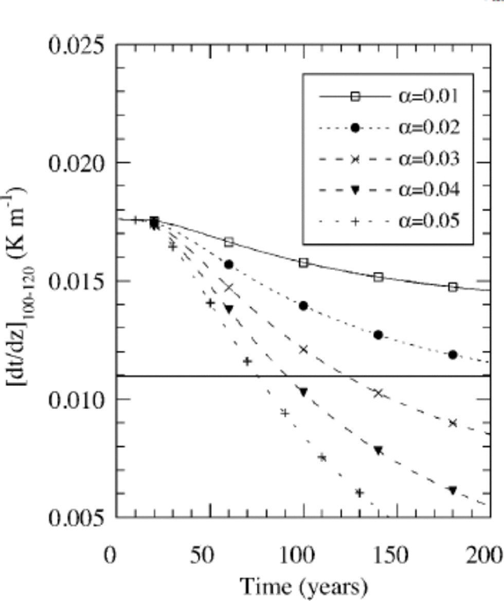
The results presented in Figure 5 show that an observed gradient of 0.01Km^–1 can be explained by a perturbation at the surface, even if the geothermal heat flux is 37.5 mWm^–2, instead of the lower value of 25 mWm^–2 which we used in the previous experiment (Fig. 4) to explain the gradient in the upper half of the profile. Figure 6 shows how the gradient near the bottom reduces for five different rates of increase in the 15m temperature. One can observe that, in the case of a larger perturbation, the gradient is reduced faster. With a slow increase of 1K per 100 years it takes a very long time for the gradient to reduce to 0.01 Km^–1. A perturbation of 4K per 100 years leads to a 50% reduction in ±100 years.

Fig. 6

The evolution of the temperature gradient in the 100– 120 m depth interval for an increase in temperature of 0.01– 0.05Ka^–1. Parameters: H = 126.5 m, G = 37.5 mWm^–2, w_s = –0.38m a^–1, linear profile.

In summary, the results obtained so far indicate that the increase in temperature in the upper half of the profile can be explained by a temperature increase, but one needs an extremely low value for the geothermal heat flux (Fig. 4 and 5). on the other hand, the calculations in Figures 5 and 7 suggest that it is possible to explain the low observed gradient near the bottom, even without an extremely low value for the geothermal heat flux.

A more rigorous treatment of the time-dependent solutions is to optimize the parameters such that the rms error between observations and measurements along the entire borehole is minimized. for this purpose the five-dimensional search space determined by

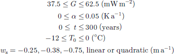
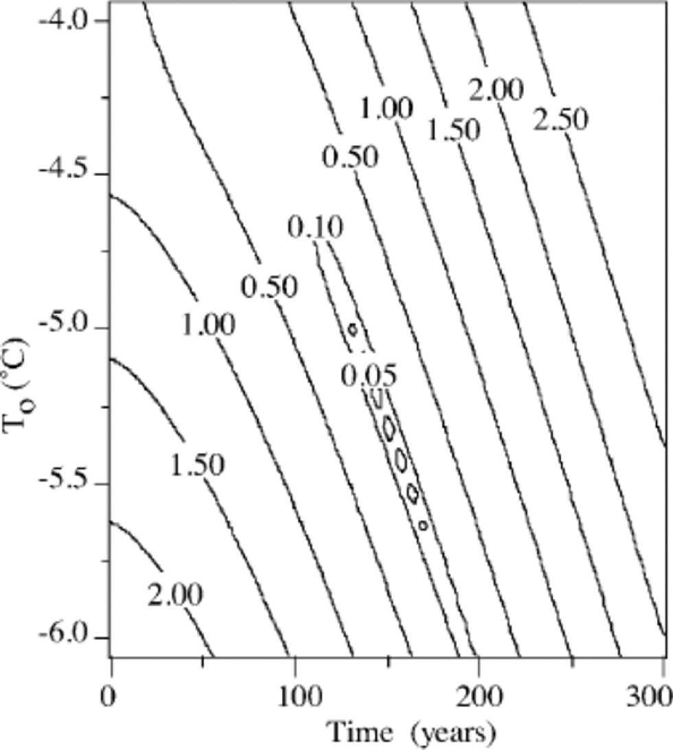
has been screened for optimal solutions. Figure 7 shows a typical result for G = 37.5 mWm^–2, α = 0.02 Ka^–1, w_s = –0.38ma^–1 and a quadratic profile. It is obvious that there is a narrow time band with optimal solutions for a given setting of G, α, W, T₀. A minimum rms error of 0.022 K is found for the above-mentioned parameter setting 102 years after the start of the perturbation. Nevertheless, small changes of T₀ still yield reasonable results, but at different times. However, this does not significantly affect the optimal value for α, which is of primary interest. Differences between solutions are not always statistically significant, so it does not make sense to define one single best solution. Results are, for example, not very sensitive to the magnitude of the vertical profile or the shape of the vertical profile, but for the parameter of key interest, α, sensitivity is higher.

Fig. 7

Typical example of the rms error between the observations and the calculations for the variables T₀ and t. the other parameters are constant: H =126.5 m, G = 37.5 mW m^–2, α = 0.025K a^–1, w_s =–0.38 m a^–1 and a quadratic profile.

The best solutions in the search space defined above are presented in Figure 8a. It turns out that the geothermal heat flux should be around 37.5 mWm^–2 and the rate of temperature increase 0.025 Ka^–1. Slightly better profiles can be found if a smaller value is used for the geothermal heat flux, but this seems to contradict the sparse data on the geothermal heat flux. Reference LiestølLiestøl (1977) presented temperature profiles in Svalbard which indicated a geothermal heat flux of 40 mWm^–2, but these measurements are only approximately comparable since they were made in other parts of the island.

Fig. 8

Optimal solutions for different vertical velocity profiles. the geothermal heat flux is 37.5 mW m^–2 for (a, c) and 50 mW m^–2 for (b). H =126.5 m, α = 0.025 K a^–1 for (a, b) and α = 0.02Ka^–1 for (c). the year mentioned in the legend is the elapsed time (t) for the optimal solution (see Equation (5)). the left column shows the absolute temperatures, and the right column the difference between observed and modelled temperatures.

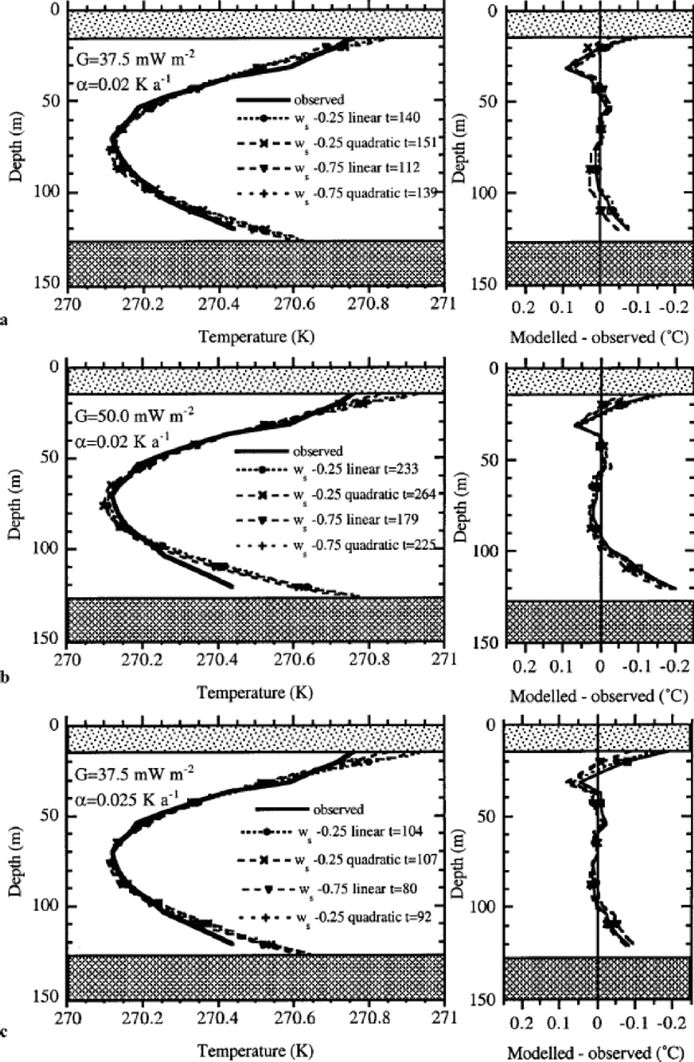
Figure 8c shows the optimal solutions for somewhat higher values of the temperature trend. Results are somewhat poorer than presented in Figure 8a, but differences between the solutions in Figure 8a and c are not significant.

The statistically best parabolic fit to the measurements yields a rms difference of 0.020 K, whereas the optimized model yields 0.022 K. the small remaining difference between measurements and calculations can be attributed to noise in the observations or a more complicated temperature increase in time. One cannot expect a statistically better result from the advection diffusionmodel used.

Larger values for the geothermal heat flux give poorer results, as can be observed in Figure 8b for G = 50 mWm^–2. All profiles are too steep near the bottom, irrespective of the assumptions for the vertical profile, and also show a temperature minimum that is both deeper and colder than observed. the experiments presented in Figures 8 and 9 show the best statistical solution within the range defined. Experiments with larger values for the vertical velocity at the surface also showed that the best results are obtained for a geothermal heat flux of 37.5 mWm^–2.

Fig. 9

Mean annual air temperature at Svalbard airport (Reference Hanssen-Bauer, Solås and Steffensen.Hanssen-Bauer and others, 1990) updated with some improvements by I. Hanssen-Bauer. Mean temperature over the period 1912–96 is –6.3˚C.

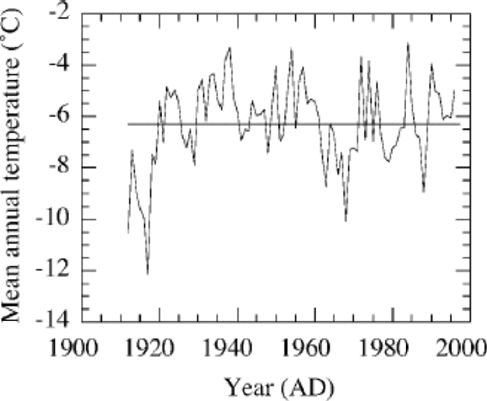
An independent test of the validity of these experiments can be obtained by a historical experiment. for this purpose we ran the model with the observations of the longest temperature record from Svalbard airport (Fig. 9), covering the period 1912–96. Before this period we used a constant temperature. the constant was optimized in order to find the best modelled temperature profile at the end of the run in 1996. the best profile was again defined as the profile with the smallest rms error between model and observations. the temperature in the 19th century was found to be 2.4K colder than the average over the period 1912–96. This experiment showed firstly that the estimated temperature increase from minimizing the rms error over the entire profile as presented in Figures 7 and 9 did not contradict the meteorological observations. Secondly, it showed that the temperature difference between the 20th and 19th centuries is about 2.4K and that the record of observations started (1912–20) in a relatively cold period, comparable to the conditions at the end of the 19th century.

5. Discussion and Conclusions

The temperature observations cannot be explained by a steady-state solution, because the difference in temperature between surface and bottom is so small and because of the fact that we observe a temperature minimum. for this reason we performed time-dependent experiments. One of the uncertainties in this kind of calculation is due to the lack of a vertical velocity profile. However, by varying the vertical velocity between 0.25 and 0.75 ma^–1 , a series of results are obtained which can be compared with the measured data. These solutions indicate that the rate of increase in temperature (α), which is of primary interest, is 0.02 –0.025 Ka^–1, but that the elapsed time (t) for the best solution varies. the elapsed time of the solutions in Figure 8a is 112–151years, and 80–107 years for the results in Figure 8c. This implies that the range of temperature increase (αt) is 2.2–3.0K for the results in Figure 8a, and 2.0–2.7K for those in Figure 8c. This paper therefore shows that ice-core temperatures from medium-length ice cores at an ice divide can be used to reconstruct the temperature over the last 100 years, even though the vertical velocity profile is not known precisely.

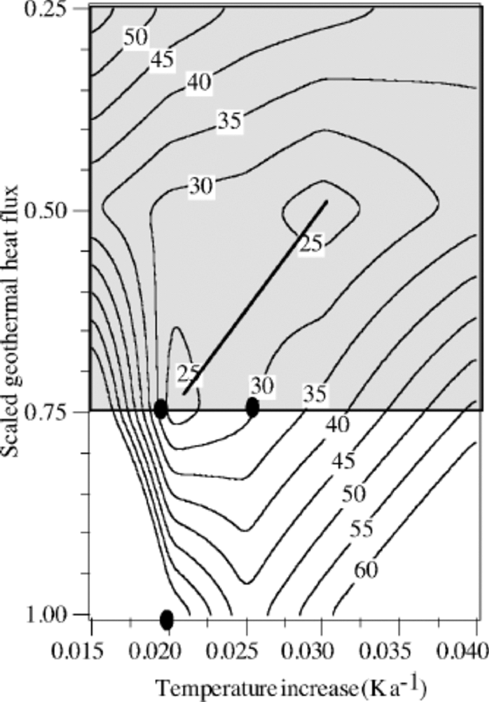
As indicated in section 4, a statistically better solution can be found for extremely low values of the geothermal heat flux. Figure 10 shows a contour diagram of the rms error as a function of the geothermal heat flux and the temperature increase. the absolute minimum is found for a scaled geothermal heat flux of 50% (=25mWm^–2). the black dots in the figure indicate the position of three optimal solutions which are presented in Figure 8a–c. Since the results presented in Figure 8a are better, especially near the bottom, than those in Figure 8c, one can conclude from Figure 10 that increasing the geothermal heat flux will not improve the results. Since we consider the temperature increase as the main parameter, and the geothermal heat flux as an important source of uncertainty, we can conclude from Figure 10 that the uncertainty in the temperature increase does not depend very much on the uncertainty in the geothermal heat flux. the line indicates the dependence of the temperature increase on the geothermal heat flux: a vertical line would indicate that it is independent of the geothermal heat flux. for a realistic range of 37.5 –50 mWm^–2, the temperature increase is 0.02–0.025Ka^–1. Higher values of the geothermal heat flux yield poor solutions, and lower values of the geothermal heat flux are considered physically unrealistic. In fact, the low values for the geothermal heat flux may be explained by the fact that we neglect the heat capacity of the underlying bedrock, which tends to suppress the heating near the bottom. Including this effect might improve the solutions near the bottom, but would not influence the main result of the calculated temperature increase.

Fig. 10

Rms error between the observations and the calculations for the variables temperature increase and scaled geothermal heat flux. the geothermal heat flux is scaled by 50 mW m^–2. Parameters: H =126.5 m, w_s = –0.38 m a^–1 and a quadratic profile. the black dots are solutions which are presented in Figure 8a–c as a function of depth. the line indicates the local minima as a function of the geothermal heat flux. the shaded area is considered physically unrealistic.

The historical experiment described at the end of section 4 showed that the temperature in the 19th century was estimated to be 2.4 K colder than the mean temperature over the period 1912–96 and that the temperature trend derived from the borehole temperatures does not contradict the meteorological observations at Svalbard airport. Air-temperature records for Svalbard over the period 1912–20 are also 2.4 Klower than the mean of the entire record, indicating that temperatures at the start of the record were comparable to temperatures at the end of the 19th century.

One might wonder whether no other temperature history can lead to a snapshot which matches the observations as well as the solution proposed here. Here, we considered first-order solutions with a simple linear trend in time. As no non-linearities are involved, one might expect to find higher frequencies with the same trend which explain the observations as well. Rapid variations in time will be diffused and will certainly lead to identical results. This, however, is of less climatological importance since it is the trend that is of primary interest. No evidence could be found for a stepwise change in the forcing at the surface.

One might also argue that changes in temperature are coupled to changes in accumulation rate and therefore influence the results obtained here by increasing the vertical advection. However, this is probably not the case, as increased accumulation will also increase the ice thickness, which compensates the effect of increased accumulation. to be able to understand fully the non-steady-state ice thickness and vertical velocity effect, one would need a thermodynamic ice-flow model. However, this is not feasible for this site due to a lack of constraints, such as ice velocity, mass-balance history and bedrock elevation.

The largest source of uncertainty is the role of refreezing. At the warmest point in the profile at 15m, the ice temperature is probably higher than the mean annual temperature (unknown at this site) due mainly to refreezing. However, structural analysis on the ice core indicates that water percolates <1m (Reference PohjolaPohjola and others, 2002). Calculations with the vertical advection and diffusion model show that nearly all heat from the refreezing in summer escapes by diffusion back to the atmosphere. Only deep percolation, to about 10 m over the short 1 month summer period, can substantially increase 15 m temperature. Our reconstructed temperature increase should be taken as a temperature increase at 15 m below the surface and not a surface temperature or atmospheric temperature. the increase in 15 mtemperature could imply either an equivalent air-temperature increase or an increase in the refreezing rate. the likelihood is that both refreezing and air temperature have changed because if the air temperature rises at this site the melting and refreezing rate will also increase. However, it is difficult to estimate the importance of changes in refreezing since the yearly mean temperature of this site is unknown, and our calculated trend is therefore an upper limit for the increase in air temperature.

Finally, if we consider the solutions presented in Figure 8a and c as the best solutions, we can calculate the temperature evolution near the bottom in the future, under the assumption that we neglect the heat generation from melting of the permafrost layer. We speculate that, roughly 90 years from now, temperatures near the bottom will be at pressure-melting point. This means that the increasing temperatures near the surface as reconstructed will probably lead to changes in the dynamics of this icefield in the near future.