1. Introduction
Chronic diseases, characterized by prolonged and often irreversible health conditions, have become a major global health concern, contributing significantly to healthcare expenditures (Yach et al., Reference Yach, Hawkes, Gould and Hofman2004). Modeling the healthcare cost data for chronic diseases pose a substantial challenge for actuaries in determining appropriate premiums, as the data are typically collected from multiple sources, such as public health institutions, insurers, and clinical diagnosis centers, resulting in high-dimensional risk characteristics (Alanazi, Reference Alanazi2022).
Beyond direct clinical factors, healthcare costs are shaped by patients’ self-perceptions (MacLeod et al., Reference MacLeod, Yang, Oakes, Connelly and Natarajan2016). Derived from structured questionnaires, these psychological constructs reveal multidimensional behavioral patterns that enrich traditional clinical metrics. Such questionnaires, commonly used in chronic disease management, assess factors like adherence to treatment protocols, dietary habits, exercise routines, and patients’ interpretations of health indicators, such as laboratory results or physical examinations. Patients with a deeper understanding of their condition tend to provide more consistent responses to related items, naturally forming covariate clusters. For instance, items related to dietary habits or exercise routines often show uniform answering tendencies, whether all correct or incorrect, highlighting underlying behavioral coherence.
Incorporating self-perception data into healthcare cost models is fraught with methodological challenges, particularly given the high-dimensional nature of survey-based covariates, which often exhibit strong correlations within behaviorally defined clusters. These interrelationships complicate predictive modeling, as conventional regularization methods like Lasso or Ridge regression treat covariates as independent, failing to capture the structured interdependencies inherent in self-perception data. Existing research has focused on low-dimensional covariates (Fellingham et al., Reference Fellingham, Kottas and Hartman2015; Shi and Zhang, Reference Shi and Zhang2015; Duncan et al., Reference Duncan, Loginov and Ludkovski2016; Richardson and Hartman, Reference Richardson and Hartman2018) or applied regularization to high-dimensional insurance data (Devriendt et al., Reference Devriendt, Antonio, Reynkens and Verbelen2021; Fung et al., Reference Fung, Tzougas and Wüthrich2023), yet these approaches neglect the latent structure of behavioral clusters. This limitation forces mutually informative covariates, such as those tied to lifestyle choices or treatment perceptions, to compete rather than collaborate, undermining the meaningful patterns they represent.
Covariate clustering offers a promising solution, as it groups highly related covariates into clusters that reflect common behavioral patterns. Integrating this approach with regularization techniques harnesses these structures to clarify how self-perception influences healthcare costs, thus transforming a high-dimensional, unstructured problem into a manageable, interpretable framework. Several studies in the statistical literature have explored this within the generalized Lasso regression framework, such as Witten et al. (Reference Witten, Shojaie and Zhang2014), Hallac et al. (Reference Hallac, Leskovec and Boyd2015) and Zhu (Reference Zhu2017). And more recently, Andrade et al. (Reference Andrade, Fukumizu and Okajima2021) introduced logistic regression models with convex covariate clustering for classification. These frameworks shrink coefficients for similar covariates based on the prior expert information, providing an analytical approach for modelling questionnaire-based healthcare data. We can then investigate complex relationships among high-dimensional features by leveraging graph-based methods and gain more insights into chronic disease progression with associated costs.
Another challenge for actuaries is the presence of unobserved heterogeneity, which can result in different effects of covariates on the response, especially in scenarios where risk characteristics impact healthcare costs differently for high-risk and low-risk patients. It frequently results in multi-modal distributions, making statistical inference difficult and highlighting the importance of identifying subgroups within the population (Kurz and Hatfield, Reference Kurz and Hatfield2019; Chen et al., Reference Chen, Tran-Dinh, Kosorok and Liu2021). One approach to address this is treating the outcome data as a mixture of several subgroups, each with its parameters, and fitting a finite mixture of regression (FMR) model. For instance, Atienza et al. (Reference Atienza, Garca-Heras, Muñoz-Pichardo and Villa2008) modeled hospital length of stay within diagnosis-related groups using a mixture of Gamma, Weibull, and Lognormal distributions. Similar methodologies, such as predictive models based on convolutive mixtures distributions (Ickowicz and Sparks, Reference Ickowicz and Sparks2017) or the use of Dirichlet mixture models for healthcare cost modeling (Fellingham et al., Reference Fellingham, Kottas and Hartman2015; Richardson and Hartman, Reference Richardson and Hartman2018), employ nonparametric models that can adapt to various distribution shapes. These approaches highlight the necessity of FMR models in healthcare utilization modeling, as they can effectively capture the underlying heterogeneity of patient populations, account for varying risk profiles, and model the diverse distributional shapes that typical healthcare utilization data often exhibit. In addition, regularization approaches in FMR models have been introduced to address the challenge of high-dimensional correlated covariates (Khalili and Chen, Reference Khalili and Chen2007; Khalili and Lin, Reference Khalili and Lin2013), with the
 $\ell_p$
regularization term being a particularly popular choice. More recently, a mixture Gamma regression model was proposed to fit heavy-tailed insurance claim data with neural networks, allowing for the detection of non-linear regression patterns (Delong et al., Reference Delong, Lindholm and Wüthrich2021). Building on these advancements, we can develop a predictive model that integrates covariate clustering with subgroup analysis, allowing clustering patterns to vary across subgroups to reflect distinct behavioral dynamics within chronic disease populations. For instance, the clustering structure of covariates and their impact on healthcare costs may differ between high-risk and low-risk subgroups, requiring separate consideration.
In this paper, we propose a novel statistical framework that integrates covariate clustering techniques into the FMR model to account for the impact of clustered covariates on specific subgroups within the dataset. The proposed approach builds on the work of Andrade et al. (Reference Andrade, Fukumizu and Okajima2021), which clusters the regression coefficients of covariates using pair-wise fused penalty. Specifically, our framework starts with an FMR model based on the exponential family of distributions, where the outcome is treated as a mixture of different subgroups. Each subgroup is assumed to be an underlying distribution with its own set of parameters, and the mean parameter of each distribution is determined by a combination of the covariates. To obtain the covariate clustering results during mixture regression, two convex penalty terms are introduced to the log-likelihood function, regularizing the model fit (the
 $\ell_2$
norm of the coefficients) and the distance of similarity between covariates (the
 $\ell_1$
norm of the difference of pair-wise coefficients). The proposed model adaptively explores the pair-wise structure of a large number of highly correlated covariates by shrinking group-specific coefficients in different mixture components. Its versatility allows applications to one-dimensional (i.e., non-mixture) scenarios where the observed sample exhibits weak heterogeneity. Our work can be seen as an extension of regression framework with a convex clustering method discussed in Chen et al. (Reference Chen, Huang, Chan and Yau2019) and Cheng et al. (Reference Cheng, Feng, Li and Wu2022).
Regarding inference, we propose a specialized expectation-maximization-alternating direction method of multipliers (EM-ADMM) algorithm to solve the complex optimization problem. In this algorithm, we implement an ADMM at the M-step of the EM algorithm, deviating from the use of Newton–Raphson optimization for estimating unknown parameters. The ADMM algorithm exhibits favorable properties for objective functions featuring
 $\ell_p \ (p\ge1)$
regularization terms, as demonstrated by Boyd et al. (Reference Boyd, Parikh, Chu, Peleato and Eckstein2011) and Chi and Lange (Reference Chi and Lange2015). Moreover, these regularizations can shrink some pairwise differences of the estimated parameters to zero. To achieve satisfactory covariate clustering results for each component in the mixture model, we set the penalty imposed on the regression coefficients within each component of the FMR model to be proportional to the mixture weight, aligning with the approach of Khalili and Chen (Reference Khalili and Chen2007).
Our research makes several significant contributions to the literature. First, we propose a comprehensive framework for modeling healthcare costs, addressing the complexities of heterogeneous samples and high-dimensional, correlated questionnaire data. Our approach employs a dual-structured learning strategy: (1) Behavioral Pattern Preservation: By incorporating convex clustering penalties within each mixture component, we automatically group covariates sharing common risk signatures, thereby preserving the integrity of self-perception constructs; (2) Heterogeneity-Aware Clustering: Unlike conventional clustering techniques, our framework permits covariate groupings to vary across population subgroups, acknowledging that behavioral patterns differing between high-risk diabetics and low-risk patients may exhibit distinct clustering structures. To our knowledge, this represents the first integration of covariate clustering with subgroup analysis in the fields of biostatistics and insurance. Second, we introduce a novel EM-ADMM algorithm for statistical inference, offering a distinctive advancement in actuarial science. We provide a detailed discussion of its implementation and convergence properties, with its effectiveness and robustness validated through simulation studies and real-world applications. Third, we analyze a diabetes dataset integrating multi-source data, including demographic, clinical, and questionnaire-based self-perception metrics, to enhance chronic disease management for the benefit of policyholders and insurers alike. By combining covariate clustering with interpretable techniques such as network analysis, we uncover variations in healthcare costs driven by patients’ diabetes knowledge and their underlying behavioral structures.
The remainder of this paper is organized as follows: Section 2 presents the data structure and characteristics. Section 3 details the methodology, presenting a regression analysis framework suitable for datasets with unobserved heterogeneity and high-dimensional covariates. Additionally, it outlines the proposed EM-ADMM algorithm designed for solving the optimization problem. Section 4 conducts simulation studies to verify the performance of the proposed model. Section 5 offers empirical results, providing an in-depth analysis of healthcare costs for diabetes patients. Section 6 concludes the paper. To enhance accessibility for practitioners, we provide the R programming codes for implementation, available at https://github.com/huangyf2217/FMR-covariates-clustering.
2. Data characteristics
In this study, we analyze healthcare cost data for 5961 Chinese diabetes patients from the year 2018. This dataset was compiled from three sources: hospital databases that provide personal demographic information, clinical diagnosis center databases that document diagnostic test results, and insurance company databases that include patient questionnaires measuring patients’ self-perceptions of diabetes. Each observation records a patient’s annual treatment and hospitalization costs realated to diabetes, which is a positive amount covered by commercial health insurance after deducting basic social health insurance. In addition, the insurance company conducts a questionnaire survey for each patient to assess their knowledge of diabetes. The survey consists of 26 main multiple-choice questions with a total of 111 options and records whether each option is answered correctly by the patient (0 for incorrect, 1 for correct). The questionnaire covers topics such as patients’ attitudes toward diabetes, awareness of medication and proper diet. And those with better knowledge are more likely to comply with treatment plans and engage in proactive self-management, thereby reducing the risk of complications and long-term costs. Variations in patient perceptions may significantly impact healthcare costs, highlighting the importance of considering these differences when developing cost prediction models for insurers and healthcare providers.
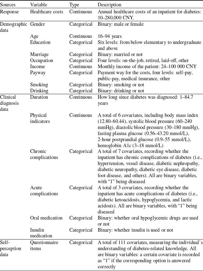
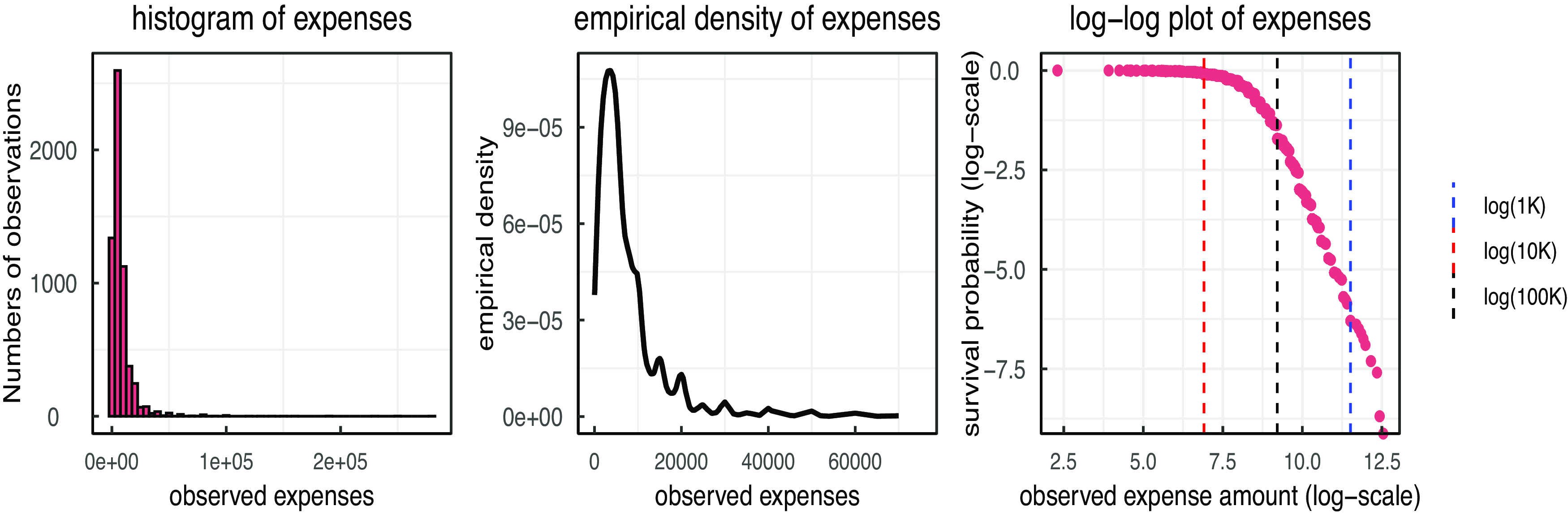
Table 1 provides an overview of the 139 covariates detailing the risk factors, and Figure 1 illustrates the empirical distribution of healthcare costs. The log–log plot shows a linear trend in the largest 10% of the tail, indicating a heavy-tailed characteristics. Additionally, the density function is highly skewed and, to some extent, multi-modal; but the subsequent peaks are not significant. The minimum healthcare cost is 10 CNY because in China, commercial health insurance pays after social health insurance reimbursement. And there are only five observations with healthcare costs below 100, which have a negligible impact on the modeling results, so we directly use it in the study.
Description of variables in diabetes dataset.

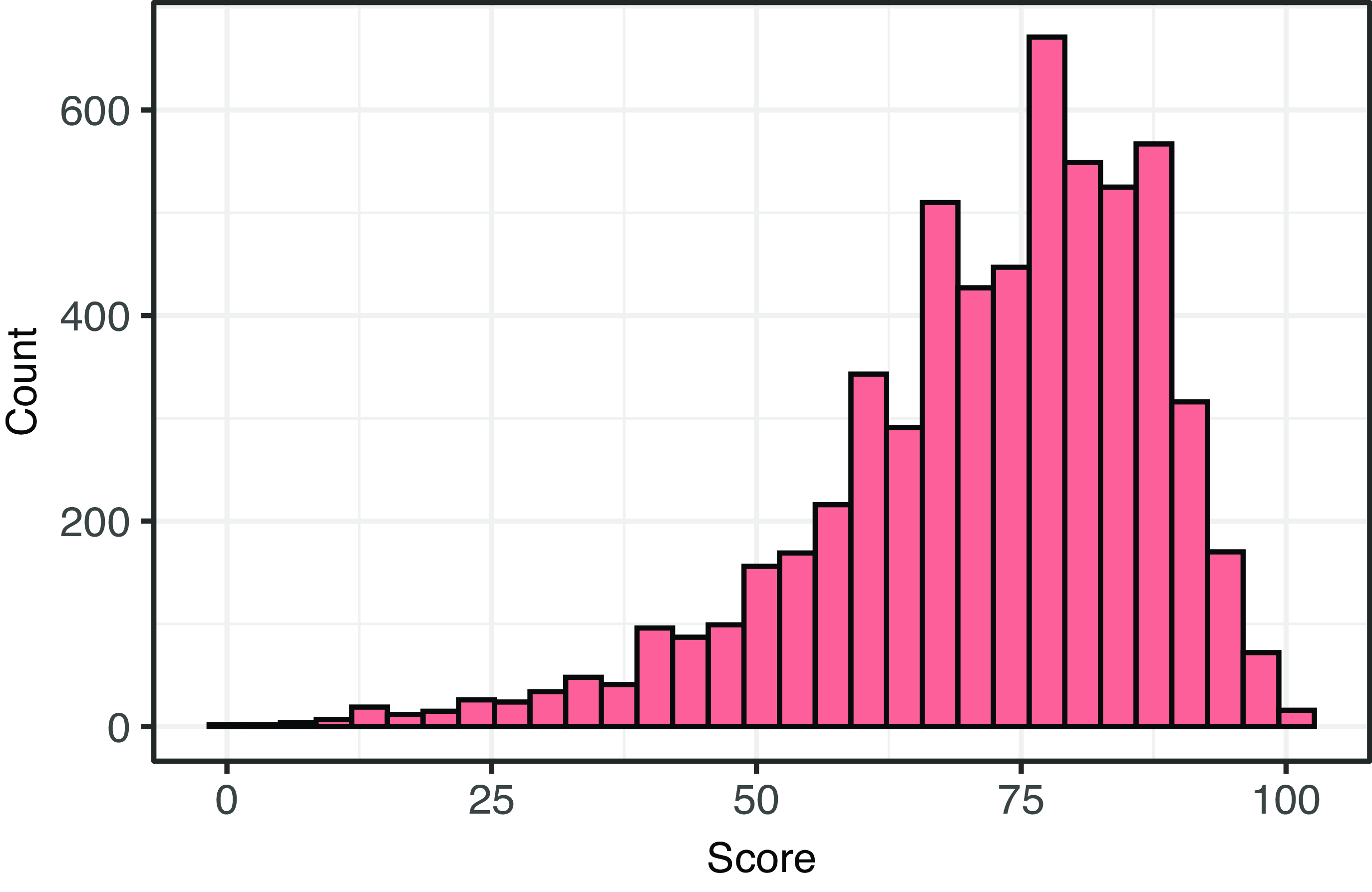
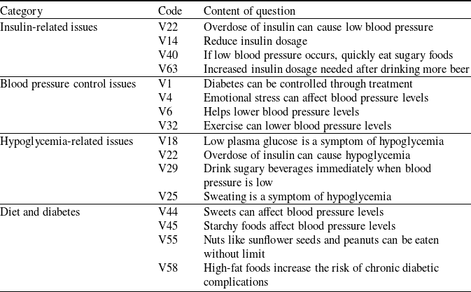
Figure 2 displays the histogram of the patients’ questionnaire scores, where each score represents the total number of correct responses out of the 111-option survey. A higher score reflects a better understanding of diabetes. Table 2 presents some of the questions, which we manually categorized based on their content. Further analysis of patients’ responses within the same categories revealed a significant positive correlation, indicating that questions in the same category are often answered correctly or incorrectly together.
3. Methodology
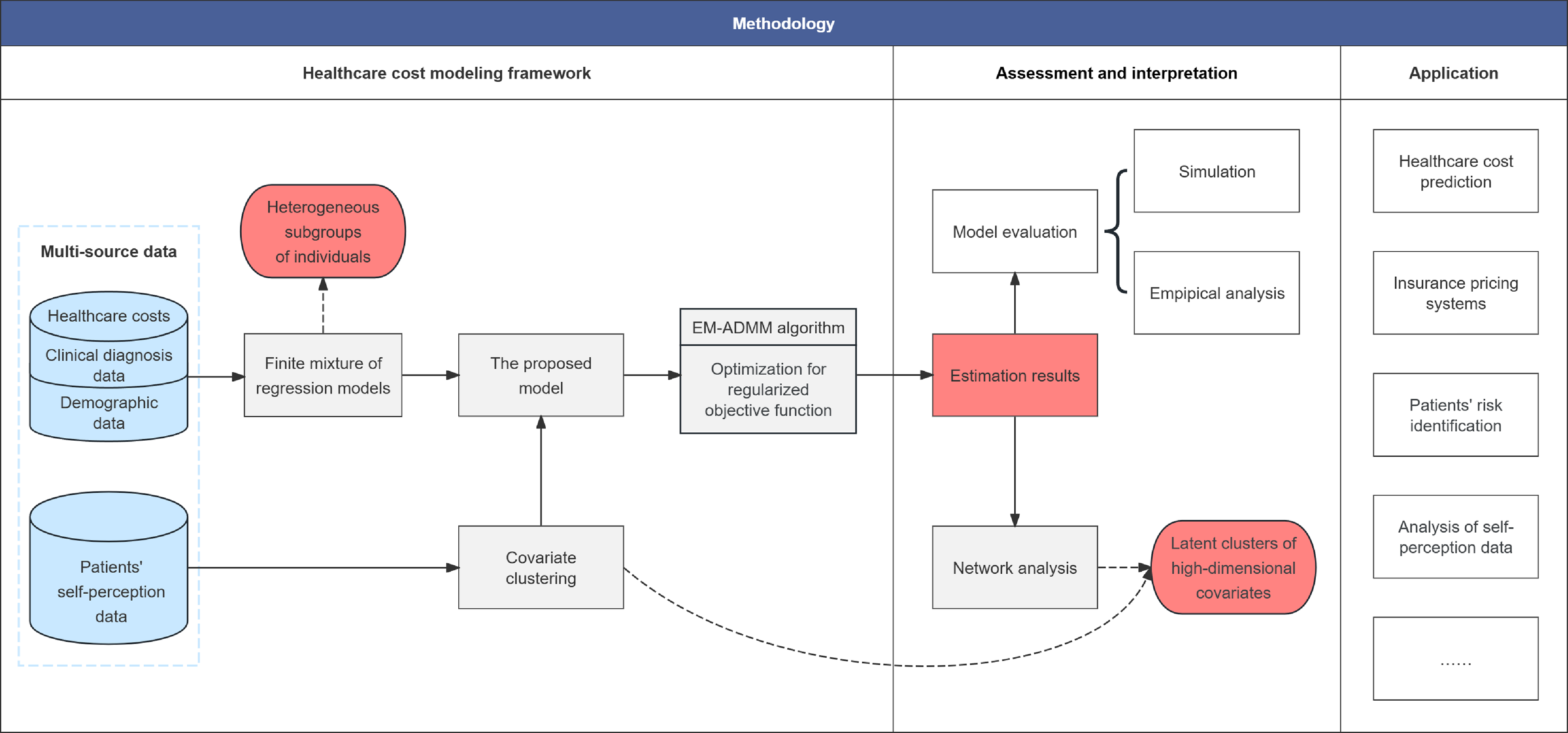
Figure 3 illustrates the general process for modeling multi-source, high-dimensional, and heterogeneous healthcare cost data in this paper. We first established an FMR of generalized linear model after cleaning and summarizing the dataset and further introduce the convex covariate clustering approach to identify clusters of the covariates from the questionnaire data. By combining EM and ADMM algorithms, the proposed model can rapidly and stably obtain the parameter estimates, enabling us to interpret the structure of covariates and their relationship with healthcare costs.
Diabetes expense dataset: Left panel: histogram of the patients’ healthcare costs; Middle panel: empirical density (upper-truncated at 75,000); Right panel: log-log plot of observed expenses.

The histogram of the patients’ questionnaire scores, the mean is 71.9 and the standard deviation is 15.9.

Examples of some questions and their corresponding categories in questionnaire data. Note that the questions within each category are not necessarily limited to those listed in the table, and the categorization may vary.

3.1. Finite mixture of regression models
Let’s assume that the healthcare cost of each patient is positive random variable (response variable), denoted as Y in the paper;
 $\boldsymbol{x} = (x_1,x_2, ...,x_p)$
is the p-dimensional covariate vector representing risk factors related to chronic disease, which can be continuous or discrete (binary) types.
Generally, the unobservable latent factors in heterogeneous response variable can be distinguished by the mixture of underlying distributions. In GLMs, Y comes from a parametric exponential family
 $\mathbb{F} = \left\{ \,f(y; \mu,\phi); (\mu, \phi) \in \mu \times \left(0, +\infty \right) \right\}$
, where
 $\mu$
is the mean parameter and is often expressed as a function of the covariates (i.e.,
 $\mu:=\mu(\boldsymbol{x})$
), and
 $\phi$
is the dispersion parameter. Then, the conditional density function of Y given
 $\boldsymbol{x}$
has the form, extending the above structure to a FMR model:
 \begin{equation} f_{\text{mix}} \left(y \left| \boldsymbol{x}, \boldsymbol{\omega}, \boldsymbol{\beta}_0, \mathbf{B}, \boldsymbol{\phi} \right. \right) =\sum_{h=1}^H {\omega_h} \,{f\left(y \left| \mu_h(\boldsymbol{x}), \phi_h \right. \right)},\end{equation}
where
 $\mu_h(\boldsymbol{x}) = g^{-1}(\beta_{0,h} + \boldsymbol{x}^T \boldsymbol{\beta}_h)$
has a linear relationship with covariates through the link function
 $g(\!\cdot\!)$
.
 $\boldsymbol{\beta}_0 = \left(\beta_{0,1},\beta_{0,2},\ldots,\beta_{0,H} \right)^T \in \mathbb{R}^{1\times H}$
and
 $\mathbf{B} = (\boldsymbol{\beta}_1, \boldsymbol{\beta}_2, \ldots, \boldsymbol{\beta}_H)^T \in \mathbb{R}^{p\times H}$
contain the intercept terms and regression coefficients, respectively, where
 $\boldsymbol{\beta}_h = (\beta_{1,h}, \beta_{2,h}, \ldots, \beta_{p,h})$
is the vector of regression coefficients in the h-th component;
 $\boldsymbol{\phi} = \left(\phi_1,\phi_2,\ldots,\phi_H \right)^T\in \mathbb{R}^{1\times H}$
represents the dispersion parameters of all H components. The component weight
 $\boldsymbol{\omega} = \left(\omega_1,\omega_2,\ldots,\omega_H \right)^T$
satisfies the constraints
 $\omega_h \gt 0$
and
 $\sum_{h=1}^{H}\omega_{h}=1$
, so the mixture density function is actually the weighted sum of all components’ densities. The form of
 $f(\!\cdot\!)$
can vary according to the response variable.
Given a sample of observations
 $\{(\boldsymbol{x}_1,y_1),(\boldsymbol{x}_2,y_2),...,(\boldsymbol{x}_n,y_n)\}$
, the (penalized) log-likelihood function of the FMR model can be designed as follows:
 \begin{align} \ell_n(\boldsymbol{\Psi})&=\sum_{i=1}^n\log f_{\text{mix}} \left(y_i \left| \boldsymbol{x}_i, \boldsymbol{\omega}, \boldsymbol{\beta}_0, \mathbf{B}, \boldsymbol{\phi} \right. \right)=\sum_{i=1}^n\log \sum_{h=1}^H {\omega_h}{f\left(y_i \left| \mu_h(\boldsymbol{x}_i), \phi_h \right. \right)},\end{align}
 \begin{align} \breve{\ell}_n(\boldsymbol{\Psi})& = \ell_n(\boldsymbol{\Psi}) - p_n(\boldsymbol{\Psi}), \\[8pt]\nonumber\end{align}
where
 $\boldsymbol{\Psi} := \left(\boldsymbol{\omega}, \boldsymbol{\beta}_0, \boldsymbol{\beta}, \boldsymbol{\phi} \right)$
,
 $\boldsymbol{x}_{i}=(x_{1,p},...,x_{i,p})$
is the p-dimensional covariates vector, and the regularization term is defined as
 $p_n(\boldsymbol{\Psi}) = \gamma \sum_{h=1}^H {\omega_h}{\left\| \boldsymbol{\beta}_h \right\|_{2}^{2}}$
with
 $\gamma$
being a nonnegative regularization parameter. The weighted
 $\ell_2$
norm shrinks the insignificant parameters in each component, which improves the model’s ability to recognize important covariates and is in line with the common practice (Khalili and Chen, Reference Khalili and Chen2007). The number of subgroups H and the corresponding underlying distributions are usually prespecified, which is usually not too large in healthcare cost modeling.
3.2 Convex covariate clustering
To analyze the effects of covariates in different components, we start by identifying the covariates with similar semantics or values, then clustering them and assigning the same regression coefficients.
The newly proposed framework for healthcare data analysis. The blue boxes represent the datasets, the gray boxes indicate the corresponding modeling techniques, and the red boxes denote the model’s results.

Suppose a similarity matrix
 $\mathbf{S}=\{s_{j,k}\}_{p \times p}$
is given a priori, where the element
 $s_{j,k}$
defines the similarity measure between the covariate j and k, as known to the experts. And generally,
 $s_{j,k} = s_{k,j}$
holds. In the graphical interpretation of clustering, the similarity matrix can be viewed as an undirected weighted graph, in which each covariate corresponds to a node, and an edge exists between nodes j and k whenever
 $s_{j,k} \gt 0$
.
Following the idea of Andrade et al. (Reference Andrade, Fukumizu and Okajima2021), we further introduce a similarity regularization term in (3.3), and the penalized objective function is then defined as
 \begin{equation} \widetilde{\ell}_n(\boldsymbol{\Psi}) = \breve{\ell}_n(\boldsymbol{\Psi}) - \frac{v}{2} \sum_{h=1}^{H} \sum_{j,k \in I} \omega_{h} s_{j,k} \lvert{\beta}_{j,h} - {\beta}_{k,h}\rvert, \end{equation}
where
 $I = \left\{1,2,...,p\right\}$
is the index set of covariates,
 $\lvert{\beta}_{j,h} - {\beta}_{k,h}\rvert$
measures the Euclidean distance between the effects of any pair of two covariates j and k in the h-th component, and v is a nonnegative tuning constant. The distance will be penalized by
 $s_{j,k}$
under this setup, thus tending to make the covariates with higher similarity obtain the same coefficients.
By adjusting the magnitude of v, we can make the coefficients
 $\hat{\beta}_{j,h}$
and
 $\hat{\beta}_{k,h}$
of similar covariates approach each other while maximizing the objective function (3.4). This utilizes the information from the response variable to guide the covariate clustering process. Note that the two regularization terms are both set to be proportional to the component weight
 $\omega_h$
, we can obtain distinct clustering and estimation results for each subgroup’s covariates. Specifically, if we set
 $H=1$
(i.e., not considering the heterogeneity in the population), the proposed framework is equivalent to adding covariate clustering in traditional GLMs.
Remark 1. In the real-data application described in Section 2, we add penalties to the 111 binary questionnaire covariates of patient responses, aiming to correlate higher correctness rates with reduced healthcare costs due to enhanced diabetes knowledge. A simpler example to illustrate the proposed model is given with the case
 $H=1,p=2$
and
 $\gamma=0$
, in which we only have two covariates with the following penalized objective function, that is,
 \begin{align} \log \mu_i &= \beta_0 + \beta_1 x_{i1} + \beta_2 x_{i2},\end{align}
 \begin{align}\widetilde{\ell}_n(\boldsymbol{\Psi}) &=\sum_{i=1}^n\log{f\left(y_i \left| \mu(x_{i1}, x_{i2}), \phi \right. \right)} - \frac{v}{2} s_{1,2} \lvert{\beta}_{1} - {\beta}_{2}\rvert, \\[8pt]\nonumber \end{align}
where
 $x_{i1}, x_{i2}\in \left\{0, 1\right\}^2$
denotes whether the questions answered correctly by patient. Sometimes the two covariates may represent similar topics, such as (1) increased physical activity can cause hypoglycemia and (2) drinking can cause hypoglycemia, patients are likely to answer these questions correctly or incorrectly simultaneously (i.e.,
 $x_{i1} = x_{i2}$
). Then our framework will suggest grouping similar domain knowledge to characterize their combined effect on healthcare costs, which is equivalent to transforming (3.5) into
 $\log \mu_i = \beta_0 + \widetilde{\beta}(x_{i1} + x_{i2})$
. By avoiding potential collinearity issues, this method is expected to be more accurate than modeling the two covariates separately. It can also reduce the impact of individual observations’ randomness in single covariates on the prediction results.
Remark 2. Our framework is not only applicable to
 $0/1$
type covariates but can also be extended to more application scenarios, such as multi-level categorical covariates (Avanzi et al., Reference Avanzi, Taylor, Wang and Wong2024) or spatial covariates (Halder et al., Reference Halder, Mohammed, Chen and Dey2021). By setting
 $\mathbf{S}=\{s_{j,k}\}_{p \times p}$
as a spatial weighting matrix, the effects of similar regions can be clustered and estimated collectively.
3.3. Optimization with the EM-ADMM algorithm
For simple FMR models, the EM algorithm is a convenient tool to solve the parameter estimation problem (Dempster et al., Reference Dempster, Laird and Rubin1977). This algorithm is generally divided into two steps: computing the conditional expectation of the log-likelihood function for a given sample data (the E-step) and, maximizing the conditional expectation and iteratively updating the estimates of
 $\boldsymbol{\Psi}$
(the M-step). However, commonly used Newton-type methods are insufficient for complex optimization with pairwise penalties, requiring improvements to the EM algorithm.
In this paper, we discuss a numerical optimization method that incorporates the ADMM algorithm into the EM iterations, enabling parameter estimation for the FMR model with covariate clustering. We call it EM-ADMM algorithm. Consistent with the EM algorithm, we first introduce the latent variables
 $u_{i,h}(h=1,2,\ldots,H)$
to indicate the subgroup of the i-th observation, where a certain
 $u_{i,h}=1$
if and only if
 $y_i$
comes from the h-th mixture component. Then based on these latent variables, the objective function (3.4) can be rewritten in the following form:
 \begin{equation} \begin{aligned} \widetilde{\ell}_n^c\left(\boldsymbol{\Psi} \right) &= \sum_{i=1}^n \sum_{h=1}^H u_{i,h} \left[\log \omega_{h} + \log{f\left(y_i \left| \mu_h(\boldsymbol{x}_i), \phi_h \right. \right)} \right] \\ &\quad - \gamma \sum_{h=1}^H {\omega_h}{\left\| \boldsymbol{\beta}_h \right\|_{2}^{2}} - \frac{v}{2} \sum_{h=1}^{H} \sum_{j,k \in I} \omega_{h} s_{j,k} \lvert{\beta}_{j,h} - {\beta}_{k,h}\rvert. \end{aligned}\end{equation}
Our proposed algorithm consists of two layers of loops to maximize
 $\widetilde{\ell}_n^c\left(\boldsymbol{\Psi} \right)$
. The outer layer is a classic EM iteration that repeatedly implements E-steps and M-steps. Assume that
 $m=1,2,\ldots,M$
represents the the number of EM iterations, the operation at the
 $(m+1)$
-th iteration is as follows.
(1) E-step. The E-step computes the conditional expectation of the function
 $\widetilde{\ell}_n^c\left(\boldsymbol{\Psi} \right)$
with respect to
 $u_{i,h}$
(referred to as the Q-function). This function has a definition of:
 \begin{equation} \begin{aligned} Q(\boldsymbol{\Psi} ; \boldsymbol{\Psi}^{(m)}) &= \sum_{i=1}^n \sum_{h=1}^H \pi_{i,h}^{(m)} \log{\omega_h} + \sum_{i=1}^n \sum_{h=1}^H \pi_{i,h}^{(m)} \log{f\left(y_i | \mu_h(\boldsymbol{x}_i), \phi_h \right)} \\ &- \gamma \sum_{h=1}^H {\omega_h}{\left\| \boldsymbol{\beta}_h \right\|_{2}^{2}} - \frac{v}{2} \sum_{h=1}^{H} \sum_{j,k \in I} \omega_{h} s_{j,k} \lvert{\beta}_{j,h} - {\beta}_{k,h}\rvert, \end{aligned}\end{equation}
which is built upon the estimation results of the previous iteration (i.e., the superscript
 $^{(m)}$
) and will be used as the objective for the M-step. And
 $\pi_{i,h}^{(m)}$
are the expectations of the unobserved
 $u_{i,h}$
as
 \begin{equation} \pi_{i,h}^{(m)}=\frac{w_h^{(m)} f\left(y_i | \mu_h^{(m)}(\boldsymbol{x}_i), \phi_h^{(m)} \right)} {\sum\limits_{h^{'}=1}^{H} w_{h^{'}}^{(m)} f\left(y_i | \mu_{h^{'}}^{(m)}(\boldsymbol{x}_i), \phi_{h^{'}}^{(m)} \right)},\end{equation}
where
 $ \mu_h^{(m)}(\boldsymbol{x}_i) = g^{-1}(\beta_{0,h}^{(m)} + \boldsymbol{x}_i \boldsymbol{\beta}_h^{(m)})$
.
(2) M-step. The M-step updates the parameters
 $\boldsymbol{\Psi}$
to maximize
 $Q(\boldsymbol{\Psi} ; \boldsymbol{\Psi}^{(m)})$
. When there are many parameters in the function, it is often possible to optimize in a sequential manner (i.e., expectation-conditional maximization, ECM).
First, we update the component weights
 $\omega_h$
like the scheme of Khalili and Chen (Reference Khalili and Chen2007):
 \begin{equation} \omega_{h}^{(m+1)} = \frac{1}{n} \sum_{i=1}^n \pi_{i,h}^{(m)}, \quad h=1,2,\ldots,H.\end{equation}
which yields a fast and relatively stable solution in our simulations.
Next, we fix
 $\omega_h = \omega_h^{(m+1)}$
and maximize
 $Q(\boldsymbol{\Psi} ; \boldsymbol{\Psi}^{(m)})$
with respect to the other parameters. Considering that the pairwise fusion penalty is not differentiable with respect to
 $\beta_{j,h}$
, we further re-parameterize the maximization of Q-function into the following optimization problem:
 \begin{align} \mathrm{minimize}_{\beta_{0}, \boldsymbol{\beta}, \phi, \boldsymbol{z}} \quad & \sum_{h=1}^H \left\{ -\sum_{i=1}^n \pi_{i,h}^{(m)} \log{f\left(y_i | \mu_h(\boldsymbol{x}_i), \phi_h \right)} + \gamma \omega_h {\left\| \boldsymbol{\beta}_h \right\|_{2}^{2}} + \frac{v}{2} \omega_h \sum_{j,k \in I} s_{j,k} \lvert z_{j,k,h} - z_{k,j,h}\rvert \right\}, \nonumber\\ \text{s.t.} \quad & z_{j,k,h} - \beta_{j,h} = 0, \quad {\forall} j,k \in \{1,2,\ldots,p\}, h \in \{1,\ldots,H\},\end{align}
where
 $\boldsymbol{z}_{h}=\{z_{j,k,h}\}$
is a set of auxiliary variables introduced for the hth component. In each of EM loops, an additional inner loop of ADMM with T iterations is required to solve the above problem. And since the parameters of each component do not interfere with each other, this problem can be optimized in a parallel manner. Under the framework of scaled ADMM (Boyd et al., Reference Boyd, Parikh, Chu, Peleato and Eckstein2011), the parameters of the h-th component during the
 $(t+1)$
-th iteration will be updated as follows:
-
• For the parameters
 $\beta_{0,h}^{(m,0)}, \boldsymbol{\beta}^{(m,0)}_{h}, \phi^{(m,0)}_{h}$
, solve the dual optimization problem (3.12): (3.12)where
\begin{align} \mathrm{argmin}_{\beta_{0,h}, \boldsymbol{\beta}_{h}, \phi_{h}} \quad g(\beta_{0,h}, \boldsymbol{\beta}_{h}, \phi_{h}) \triangleq &- \sum_{i=1}^n \pi_{i,h}^{(m)} \log{f\left(y_i | \mu_{h}(\boldsymbol{x}_i), \phi_{h} \right)} + \omega_{h} \gamma {\left\| \boldsymbol{\beta}_{h} \right\|_{2}^{2}} \nonumber \\ &+ \frac{\rho}{2} \sum_{j=1}^p \sum_{k=1}^p \left(z_{j,k,h}^{(m,t)} - \beta_{j,h} + r_{j,k,h}^{(m,t)} \right)^2. \end{align}
$\rho \gt 0$
is a predefined penalty parameter, and
$\boldsymbol{r}_{h}=\{r_{j,k,h}\}$
is a set of scaled dual variables. This problem can generally be solved using the BFGS (Broyden–Fletcher–Goldfarb–Shanno) algorithm, as for most exponential families, its derivatives can be easily computed by the chain rule.
-
• For the auxiliary variables
$\{z_{j,k,h}^{(m,t+1)}\}$
, solve the dual optimization problem (3.13): (3.13)
\begin{equation} \mathrm{argmin}_{\boldsymbol{z}_h} \quad \omega_h \frac{v}{2} \sum_{j=1}^p \sum_{k=1}^p s_{j,k} \left| z_{j,k,h} - z_{k,j,h} \right| + \frac{\rho}{2} \sum_{j=1}^p \sum_{k=1}^p \left(z_{j,k,h} - \beta_{j,h}^{(m,t+1)} + r_{j,k,h}^{(m,t)} \right)^2. \end{equation}
-
• For the scaled dual variables
$\{r_{j,k,h}^{(m,t+1)}\}$
, which is equivalent to the residual between
$\beta_{j,h}^{(m,t+1)}$
and its auxiliary variable
$z_{j,k,h}^{(m,t+1)}$
, the estimates can be easily calculated by (3.14)
\begin{equation} r_{j,k,h}^{(m,t+1)} = r_{j,k,h}^{(m,t)} + \left(z_{j,k,h}^{(m,t+1)} - \beta_{j,h}^{(m,t+1)} \right). \end{equation}


(3) Repeat E-step and M-step until the norm difference between the predicted regression coefficients of the two adjacent EM algorithms
 $\lVert \boldsymbol{\hat{\mathbf{B}}}^{(m+1)} - \boldsymbol{\hat{\mathbf{B}}}^{(m)} \lVert_{F}$
is less than the given threshold.
Proposition 1. The optimization problem (3.11) conforms to the general form of ADMM; hence, the Q-function is guaranteed to achieve conditional maximization in each M-step.
For each component h, the objective function can be simplified as
 $g_1(\boldsymbol{\psi}) + g_2(\boldsymbol{z})$
, along with the constraint
 $\mathbf{A}\boldsymbol{\psi} + \mathbf{B}\boldsymbol{z} = 0$
. Here,
 $g_1(\boldsymbol{\psi})= -\sum_{i=1}^n \pi_{i,h}^{(m)} \log{f\left(y_i | \mu_h(\boldsymbol{x}_i), \phi_h \right)} + \gamma \omega_h {\left\| \boldsymbol{\beta}_h \right\|_{2}^{2}}$
represents the first two terms of (3.11), with
 $\boldsymbol{\psi} = \{\beta_{0,h},\boldsymbol{\beta}_h,\phi_h\}$
; and
 $g_2(\boldsymbol{z}) = \frac{v}{2} \omega_h \sum_{j,k \in I} s_{j,k} \lvert z_{j,k,h} - z_{k,j,h}\rvert$
represents the last term of the function.
According to Boyd et al. (Reference Boyd, Parikh, Chu, Peleato and Eckstein2011), the convergence of ADMM requires two conditions: the first is that both
 $g_1$
and
 $g_2$
are convex, and the second is the existence of a saddle point for the unaugmented Lagrangian function
 $L_0(\boldsymbol{\psi},\boldsymbol{z},y) = g_1(\boldsymbol{\psi}) + g_2(\boldsymbol{z}) + y^T(\mathbf{A}\boldsymbol{\psi} + \mathbf{B}\boldsymbol{z})$
. The convexity requirement is easy to prove. Since the negative log-likelihood of the exponential family,
 $-\log{f(\!\cdot\!)}$
, is convex, and both the
 $\ell_1$
and
 $\ell_2$
norms are obvious convex functions, it follows that
 $g_1$
and
 $g_2$
are convex, as they are linear combinations of a finite number of convex functions.
Given that the objective function is convex and the constraints are linear, it suffices to prove that the optimization problem satisfies Slater’s condition to ensure the existence of at least one saddle point for
 $L_0$
. The matrices
 $\mathbf{A}$
and
 $\mathbf{B}$
are defined as follows:
 \begin{equation*}\mathbf{A} = \left[\begin{array}{c@{\quad}c@{\quad}c@{\quad}c@{\quad}c}\mathbf{0}_{p \times 1} & \mathbf{-1}_{p \times 1} & \cdots & \mathbf{0}_{p \times 1} & \mathbf{0}_{p \times 1} \\\vdots & \vdots & \ddots & \vdots & \vdots \\\mathbf{0}_{p \times 1} & \mathbf{0}_{p \times 1} & \cdots & \mathbf{-1}_{p \times 1} & \mathbf{0}_{p \times 1}\end{array}\right]_{p^2 \times (p+2)},\ \ \mathbf{B} = \mathbf{I}_{p^2},\end{equation*}
where in each row of
 $\mathbf{A}$
, only the element corresponding to
 $\beta_j$
has a value of
 $-1$
, and all other elements are 0. Since the matrix
 $[\mathbf{A},\mathbf{B}]$
is full rank for any positive integer p, the linear constraint system must have a solution, which guarantees the presence of at least one feasible point and thus satisfies Slater’s condition. The optimization problem (3.11) shows strong duality, and there exist
 $(\boldsymbol{\psi}^\star, \boldsymbol{z}^\star, y^\star)$
such that
 $L_0(\boldsymbol{\psi}^\star, \boldsymbol{z}^\star, y) \leq L_0(\boldsymbol{\psi}^\star, \boldsymbol{z}^\star, y^\star) \leq L_0(\boldsymbol{\psi}, \boldsymbol{z}, y^\star)$
.
Proposition 2. The EM-ADMM is essentially a variant of the ECM (Expectation/Conditional Maximization) algorithm proposed by Meng and Rubin (Reference Meng and Rubin1993). And under the update scheme for the CM-steps in this paper, it can converge properly just like the EM algorithm.
In each step of the maximization process (disregarding the effects of different components h), we decompose the parameter space as
 $\boldsymbol{\Psi} = \{\psi_1 = \omega_h, \boldsymbol{\psi}_2 = (\beta_{0,h},\boldsymbol{\beta}_h,\phi_h)\}$
so that
 $Q(\boldsymbol{\Psi}; \boldsymbol{\Psi}^{(m)})$
becomes easier to maximize for
 $\psi_1$
given
 $\boldsymbol{\psi}_2$
and vice versa. The original M-step is replaced by two CM-steps, and according to (3.10) and Proposition 1, both steps perform conditional maximization with respect to
 $\psi_1$
or
 $\boldsymbol{\psi}_2$
. Specifically, our update scheme setup guarantees that
 $Q(\psi_1^{(m+1)}, \boldsymbol{\psi}_2^{(m)}) \geq Q(\psi_1^{(m)}, \boldsymbol{\psi}_2^{(m)})$
and
 $Q(\psi_1^{(m+1)}, \boldsymbol{\psi}_2^{(m+1)}) \geq Q(\psi_1^{(m+1)}, \boldsymbol{\psi}_2^{(m)})$
. Meanwhile, it is easy to see that the two optimization processes are independent of each other. When searching for the conditional maximum with respect to one parameter, the other parameter will not restrict the search direction, namely, “space filling”. Meng and Rubin (Reference Meng and Rubin1993) proved that the ECM algorithm retains the stable convergence properties of the EM algorithm under such conditions, in particular the objective function (3.7) increasing monotonically and converging to a stationary point of
 $\widetilde{\ell}_n^c\left(\boldsymbol{\Psi} \right)$
.
Our model and algorithm are, to some extent, similar to those of Khalili and Chen (Reference Khalili and Chen2007). However, we introduce a more complex penalty term into the likelihood function to achieve covariate clustering and solve it using the ADMM algorithm.
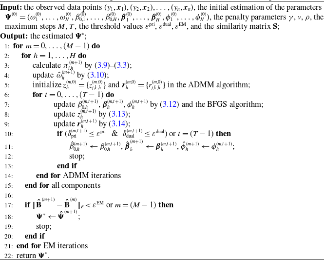
The complete EM-ADMM algorithm is provided by Algorithm 1, which is implemented in the R platform in this paper. The convergence of the algorithm is demonstrated in the simulation study; please refer to the supplementary materials for further computational details.
The EM-ADMM algorithm for FMR models with covariate clustering.

4. Simulation
A simulation study is first conducted to validate the effectiveness of the proposed framework and algorithm in covariate clustering and parameter estimation for the FMR model. We assume that the observations will be generated by a mixture distribution consisting of two components, each of which obeys a Gamma distribution but with different mean and dispersion parameters, as follows:
 \[Y_i \sim \omega_1 \text{Gamma}(y_i \left| \mu_{1}(\boldsymbol{x}_i), \phi_1 \right. ) + \omega_2 \text{Gamma}(y_i \left| \mu_{2}(\boldsymbol{x}_i), \phi_2 \right. ),\quad i = 1,\ldots, n,\]
where the mean parameters are expressed as
 $\mu_{h}(\boldsymbol{x}_i) = \exp(\beta_{0,h} + \boldsymbol{x}_i^T \boldsymbol{\beta}_h), h=1,2$
.
For this mixture Gamma model, we set the true parameter values for each component as
 \begin{align*} \text{Component} \ 1&: \omega_1=0.3, \ \beta_{0,1}=2,\ \boldsymbol{\beta}_1 = (\overbrace{\beta_{1,1},...,\beta_{5,1}}^{0.1}, \overbrace{\beta_{6,1},...,\beta_{10,1}}^{0.2}), \ \phi_1 = 0.1\\ \text{Component} \ 2&: \omega_2=0.7, \ \beta_{0,2}=1,\ \boldsymbol{\beta}_2 = (\overbrace{\beta_{1,2},...,\beta_{5,2}}^{-0.1}, \overbrace{\beta_{6,2},...,\beta_{10,2}}^{-0.2}), \ \phi_2 = 0.2;\end{align*}
which essentially assumes that these 10 covariates originate from 2 clusters, with covariates within the same cluster sharing a common effect on the outcome data, that is,
 $\boldsymbol{x}=(1, \overbrace{x_{1},...,x_{5}}^{\text{cluster 1}}, \overbrace{x_{6},...,x_{10}}^{\text{cluster 2}})$
. The regression coefficients of the covariates are completely opposite between the two components, reflecting the challenge caused by unobserved heterogeneity in healthcare cost modeling.
We then generate the dataset with a sample size
 $n=1000$
for each run of the simulation. In robust tests, the covariates
 $\boldsymbol{x}_i$
are assumed to be a set of continuous variables drawn from a multivariate normal distribution
 $\text{MN}(\mathbf{0}, \mathbf{\Sigma})$
, which has the mean of
 $\mathbf{0}$
and the covariance matrix of
 $\mathbf{\Sigma}$
.
 $\mathbf{\Sigma}$
is a
 $p \times p$
block diagonal matrix with the following structure:
 \begin{align*} \Sigma_{kk'}=\begin{cases} 0.04 & \text{if}\quad k=k',\\ 0.04\varrho & \text{if}\quad 1 \le k,k' \le 5 \ \text{or} \ 6 \le k,k' \le 10, \ k \neq k',\\ 0& \text{otherwise},\end{cases}\end{align*}
where
 $\varrho$
denotes the correlation coefficient. And we vary the value of
 $\varrho$
from the grid
 $\{0.1,0.5,0.9\}$
to reflect the influence of different covariate similarities on our model. The observations of
 $Y_i(i=1,\ldots, n)$
will be generated according to the following scenario: first, simulate a random number on the (0,1) interval to determine the latent subgroup h to which the individual belongs; then draw the value from the corresponding component
 $\text{Gamma}(y_i \left| \mu_h(\boldsymbol{x}_i),\phi_h \right.)$
.
For each simulated dataset, we first fit the correct two-component Gamma model using a wide range of tuning values for v
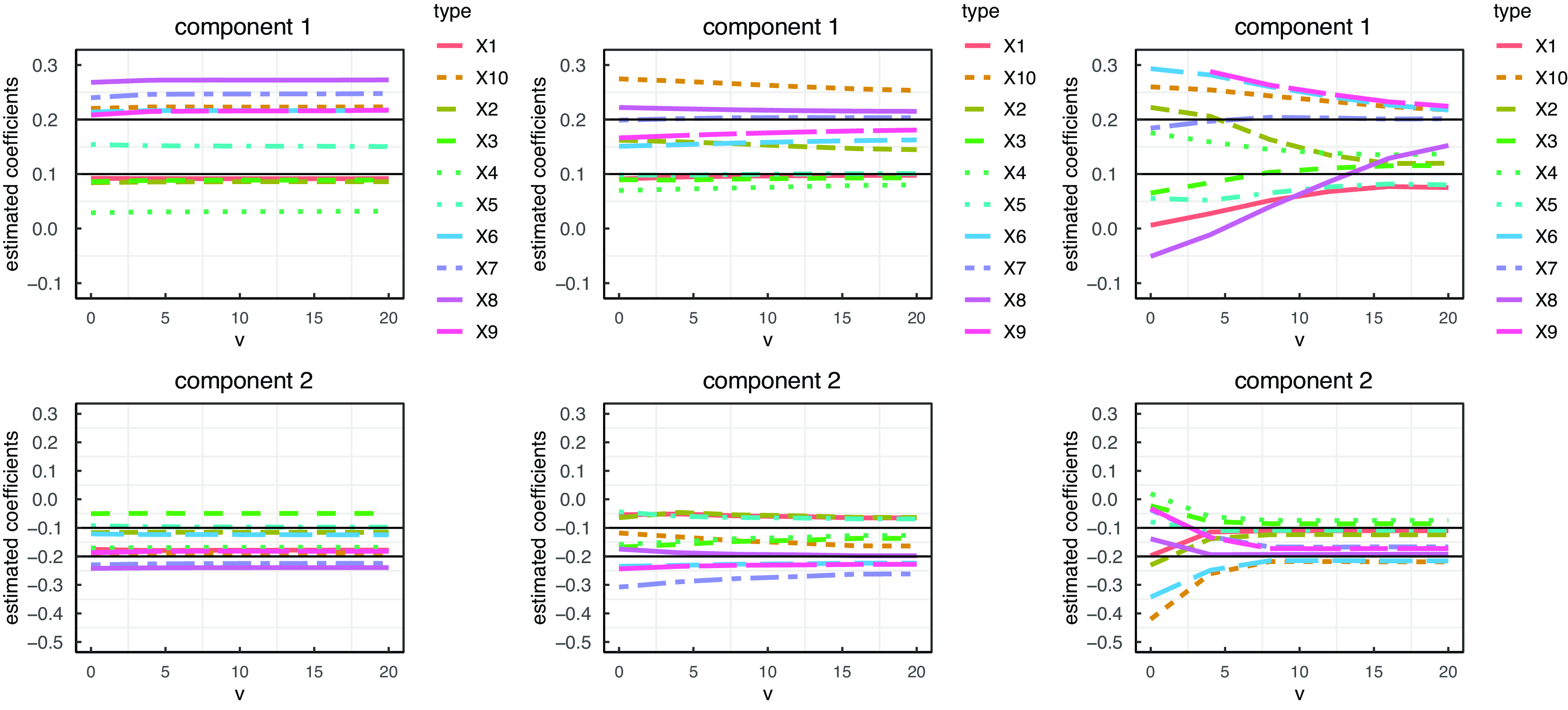
Footnote 1. Figure 4 displays the solution paths of the covariate coefficients against v under three simulated samples with
 $\varrho = 0.1, 0.5, 0.9$
. When there is indeed a certain correlation among covariates (e.g.
 $\varrho=0.5$
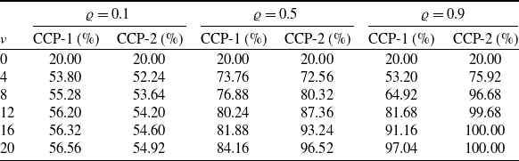
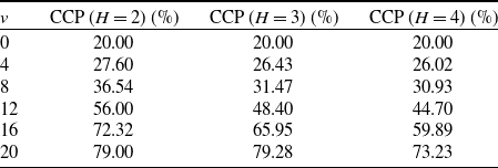
), our model can cluster them in each component and assign them the correct coefficient estimates, and the identification and clustering performance are better for the important subgroup with a larger weight. In Table 3, we report the correctly clustered proportion (CCP) of the covariates in each component, which is calculated based on the average results of 100 simulations. The CCP measures the agreement between the true and estimated clusters, and a value close to 1 is preferred. As expected, CCP-1 and CCP-2 both increase as the tuning parameter v increases, especially when the true correlation of the covariates is high.
The correct clustering proportion (CCP) in each component for Gamma mixture regressions in the case that the covariates are assumed to be grouped into two clusters. The results are averaged by repeating the simulation 100 times.

*CCP-1 and CCP-2 denote the correct clustering proportion in components 1 and 2, respectively.
The solution paths for the covariates clustering against v based on random samples with various values of
 $\varrho$
. Left panel, Middle panel, and Right panel display the estimated coefficients when
 $\varrho=0.1,0.5,0.9$
respectively. The components 1 and 2 are presented in the Top and Bottom panels. The true values of regression coefficients are marked as the black solid lines.

To examine the covariate clustering results when the distributional assumptions of the model are violated, we continue fitting the following model:
 \begin{align*} f_{mix}(y) = \sum_{h=1}^{H}\omega_h \,f_{\text{}}(y \left| \mu_{h}(\boldsymbol{x}), \sigma_h \right. ),\end{align*}
where the mean parameter is expressed as
 $\mu_{h}(\boldsymbol{x}) = \beta_{0,h} + \boldsymbol{x}^T \boldsymbol{\beta}_h$
. This setting assumes the distribution of each component to be normal (i.e., differs from the Gamma distribution of the true data), and we also experimented with different component numbers (i.e.,
 $H=2,3,4$
) to evaluate the modified model from two perspectives. Table 4 presents the CCP measures for models under different values of v. It indicates that even under incorrect distributional assumptions, our framework is still able to accurately identify the clusters to which the covariates belong. Although the accuracy of covariate clustering is affected when the model’s distributional assumption does not align with the true data (i.e., compared to Table 3, the CCP decreases under the same v), further increasing v is expected to improve this. Moreover, the clustering results are evidently best when
 $H=2$
, but even with
 $H=3,4$
, the model maintains clustering performance in redundant components.
The CCP over all components for Normal mixture regressions in the case that the covariates are assumed to be grouped into two clusters. The simulated data are generated using the same method as before, with the correlation coefficient chosen as
 $\varrho=0.9$
. The results are averaged by repeating the simulation 100 times.

5. Empirical analysis
5.1. Experimental setup
In this section, we demonstrate the superiority of the proposed covariate clustering regression model for predicting the healthcare costs in the diabetes dataset described in Section 2. To prevent overfitting, the dataset
 $\mathcal{L}(y_{i},\boldsymbol{x}_i), {0\le i\le n}$
is randomly split into a training set and a testing set at an 80:20 ratio, resulting in 4768 observations for model fitting and hyperparameter tuning, and 1193 for out-of-sample analysis. We transform the response variable into
 $y^*=y/10,000$
, normalize all continuous covariates, and convert the other (multiple) categorical covariates into dummy ones.
Model comparison is conducted in terms of goodness of fit, predictive accuracy, and discriminative ability for samples at different risk levels. Two commonly used metrics, negative log-likelihood (NLL) and pseudo R
 $^2$
, are employed to evaluate model fit. NLL can be defined as
 $-\ell_n(\boldsymbol{\Psi})$
with the set of estimated parameters, when assuming each mixture component follows a Gamma distribution, the density function f(y) in (3.2) has the form of:
 \begin{equation} f\left(y \left| \mu, \phi \right. \right) = \frac{y^{\frac{1}{\phi^2}-1} \exp\left(-\frac{y}{\mu\phi^2}\right)} {(\mu\phi^2)^{\frac{1}{\phi^2}} \ \Gamma({1}/{\phi^2})},\end{equation}
where
 $\Gamma(\!\cdot\!)$
is the gamma function. The pseudo R
 $^2$
measures the gap of log-likelihood between the saturated and predictive model. Specifically, given the true observations
 $\boldsymbol{y} = ({y}_1, \ldots, {y}_n)$
and the predictions
 $\hat{\boldsymbol{y}} = (\hat{y}_1, \ldots, \hat{y}_n)$
, where
 $\hat{y}_i = \sum_{h=1}^H \hat{\omega}_h \hat{\mu}_h(\boldsymbol{x}_i)$
, the pseudo R
 $^2$
under the Gamma distribution assumption can be expressed as:
 \begin{equation} \text{R}^2 = 1 - \frac{\sum_{i=1}^n \left[\log(y_i / \hat{y}_i) - (y_i-\hat{y}_i)/\hat{y}_i \right]} {\sum_{i=1}^n \log(y_i / \bar{y})},\end{equation}
where
 $\bar{y}$
is the sample mean of
 $y$
. A lower NLL and a higher R
 $^2$
are preferred for the model.
Regarding predictive accuracy, we use mean squared error (MSE) for point estimation accuracy and mean continuous ranked probability score (MCRPS) for distribution estimation accuracy. While MSE is easy to calculate, CRPS measures how well the overall predicted distribution takes values around the true observation (Gneiting and Raftery, Reference Gneiting and Raftery2007). Its analytical form is
 \begin{equation} \text{CRPS}(y_i, \hat{F}) = \int_{\mathbb{R}} \left[\hat{F}(y_i|\boldsymbol{x}_i) - \text{I}(y_i \leq z) \right]^2 dz,\end{equation}
where
 $\hat{F}(\!\cdot\!)$
is the estimated cumulative distribution function corresponding to (3.1), and
 $\text{I}(\!\cdot\!)$
is an indicator function. A smaller CRPS indicates a predicted distribution more concentrated around the true value. We average the CRPS across all samples to evaluate the model’s overall performance.
Finally, we use the two-way Lift metric to assess the model’s ability to discriminate risk across samples (Lee, Reference Lee2021). To calculate the Lift, we bin the samples into ten equal groups according to their predicted losses, from low to high, and then divide the average response of the top-decile group by that of the bottom-decile group. A higher Lift means that the model can better distinguish between high-risk and low-risk individuals.
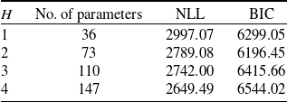
We first test FMR models with different component numbers H, using only 28 traditional risk factors. Table 5 reports the NLL and BIC of models with varying H values on the training set. Although NLL decreases as H increases, it significantly raises the number of parameters (especially with questionnaire covariates). When
 $H \geq 2$
, the decline in NLL stabilizes, and the BIC values also indicate that
 $H=2$
can balance model simplicity and capture patient heterogeneity effectively. Therefore, subsequent modeling will consider at most two mixture components.
NLL and BIC of models with different H on the training data.

Additionally, we adopt a data-driven approach that constructs the similarity matrix
 $\mathbf{S}=\{s_{j,k}\}_{p \times p}$
by computing the cosine similarity between covariates
 $x_j$
and
 $x_k$
in the training set. More sophisticated methods for defining covariate similarity are worth exploring in future research.
5.2. Comparative results
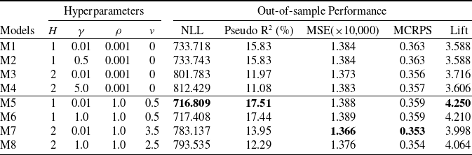
Table 6 presents the out-of-sample performance of some competing models, including conventional GLMs, ridge GLMs, and covariate clustering GLMs, as well as corresponding FMR models. Among them, M1 to M4, respectively, represent the conventional GLM (without
 $\ell_2$
-penalty and similarity penalty), ridge GLM (without similarity penalty), conventional FMR model (without
 $\ell_2$
-penalty and similarity penalty), and FMR model with
 $\ell_2$
-penalty (without similarity penalty); M5–M8 are similar to M1–M4, but they all incorporate our proposed covariate clustering framework (i.e. with similarity penalty). The Gamma distribution is used for GLMs, and the two-component Gamma mixture distribution is used for FMR models. Regarding the selection of tuning parameters, when the
 $\ell_2$
norm regularization term is considered,
 $\gamma$
is tuned from the values
 $\{0.5, 1.0, 5.0 \}$
; otherwise
 $\gamma = 0.01$
is fixed to ensure the convexity of the objective function. When the regularization term for covariate clustering is added,
 $\rho = 1.0$
is fixed, and v is tuned from the grid values
 $\{0.5, 1.0, \ldots, 4.5, 5.0 \}$
; otherwise,
 $\rho = 0.001$
, and
 $v = 0$
are fixed. We select the tuning parameters that can achieve the minimum NLL on the validated set for each model.
Diabetes expense dataset: out-of-sample performance of the eight competing models. The hyperparameters are selected through cross-validation on the training set; after determining the optimal ones, the model is retrained and evaluation metrics are calculated on the testing set.

*The optimal values of metrics are in bold.
From Table 6, we can conclude that the proposed covariate clustering method significantly improves the model’s performance for predicting the diabetes expenses characterized by a large number of highly correlated risk factors, as most of the metrics of M5–M8 (i.e. with the proposed covariate similarity penalty) are superior to those of M1–M4 (i.e. without the similarity penalty). Notably, the covariate clustering model not only accurately estimates the expected value (point estimates) but also effectively characterizes the overall distribution of the target outcome, as evidenced by the improvement in goodness of fit (NLL and pseudo R
 $^2$
) and the ability to discriminate extreme observations (Lift). This phenomenon is consistent with our expectations that the covariate clustering method is equivalent to aggregating the effects of multiple related risk factors, which eliminates the random disturbance and mutual interference among the covariates, ultimately enhancing the data. Second, once the covariates with similar or repeated effects have been clustered during the regression process, the original
 $\ell_2$
norm penalty for the compression and selection of covariates is no longer necessary. The results indicate that the performance of models {M2, M4, M6, M8} (i.e. with
 $\ell_2$
-penalty) is not as optimal as that of models {M1, M3, M5, M7} (i.e. without
 $\ell_2$
-penalty). As previously mentioned, dimensionality reduction can also be achieved by clustering similar covariates, rendering the use of the
 $\ell_2$
norm penalty unnecessary in subsequent experiments. Third, in comparing mixture and non-mixture models, it can be observed that M5 (i.e. single-component, non-mixture) exhibits the best performance in terms of goodness of fit and risk discrimination ability, while M7 (i.e. two-component mixtures) performs best in terms of prediction accuracy. Non-mixture models are effective in capturing the characteristics of diabetes expenses data when heterogeneity is insignificant, while mixture models can generally capture the majority values of the sample and have advantages in point estimation.
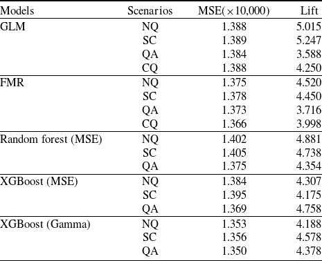
We further examine the influence of different covariate subsets on healthcare costs, which is conducted under four distinct scenarios:
-
• NQ Scenario: this scenario excludes the 111 questionnaire dummy variables from the model.
-
• SC Scenario: the total count of correct responses from the 111-question survey is included as a continuous score, a higher score indicates a better understanding of diabetes.
-
• QA Scenario: the questionnaire data are introduced as 111 dummy variables into the model.
-
• CQ Scenario: here, we perform regression while simultaneously clustering the 111 questionnaire dummy variables by the proposed framework.
In addition to the distributional regression models (i.e., GLMs and FMR), we also evaluate two machine learning models: random forest and XGBoost. Both random forest (MSE) and XGBoost (MSE) are trained using the mean squared error loss function, while XGBoost (Gamma) is trained using the Gamma deviance loss function. Optimal hyperparameters for these models are selected through a fivefold cross-validation process. The comparative results are summarized in Table 7. Note that machine learning models can only provide point estimates of the mean and, therefore, are unable to assess their performance in fitting the distribution, such as NLL, pseudo R
 $^2$
, and CRPS.
Diabetes expense dataset: out-of-sample performance of distributional regression and machine learning models in different scenarios. All models are evaluated on the testing set after tuning.

A notable finding is that, no matter distributional regression or machine learning techniques are used, the MSE values in the QA scenario are consistently lower than those in the NQ scenario, highlighting the value of incorporating patients’ self-perception into predictive models. The detailed questionnaire responses in the QA scenario also provide richer and more actionable insights than a single aggregated score in the SC scenario, which leads to lower MSE across the models. However, this trend is less pronounced in the GLM and FMR models, likely due to their limitations in handling high-dimensional covariates. The CQ scenario yields the lowest MSE for the FMR model, indicating that incorporating covariate clustering can enhance the model’s predictive performance. In fact, the CQ scenario outperforms both the NQ and SC scenarios in terms of MSE, demonstrating the advantage of covariate clustering in improving model accuracy among distributional regression models. Among all machine learning models, the XGBoost (Gamma) model applied to the QA scenario demonstrates relatively strong performance, even outperforming the FMR model in the CQ scenario. This is understandable, as XGBoost is optimized for predictive accuracy and can handle the complex relationships among covariates to some extent. However, the model lacks interpretability about insurance pricing results and cannot provide the distributional characteristics of healthcare costs, making it challenging to analyze skewness, kurtosis, and tail risk measures, which are crucial for effective risk management. Our proposed model also outperforms the random forest with a lower MSE and offers advantages in interpretability and distribution fitting.
Beyond predictive accuracy, we observe that the CQ scenario increases the lift value relative to the QA scenario among distributional regression models, improving the ability to distinguish between high- and low-risk patients. The XGBoost (MSE) model in the QA scenario achieves the highest lift among machine learning models, but its MSE does not perform as well as FMR’s CQ scenario, suggesting a trade-off between the risk discrimination ability and predictive accuracy.
5.3. Network analysis of patients’ self-perception data
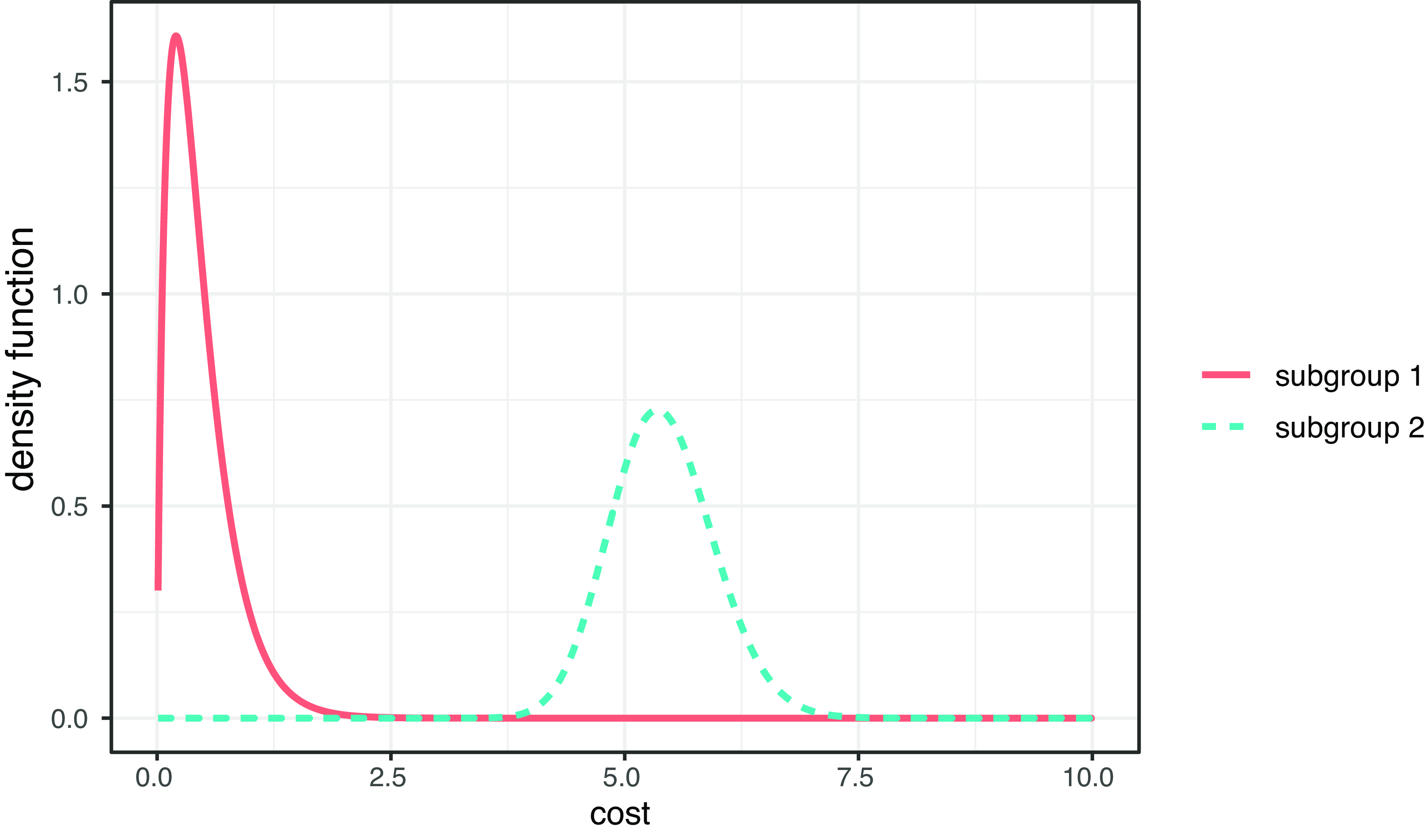
We utilize network analysis to investigate the relationships between covariates in M7. Figure 5 illustrates the density function of the cost data for two subgroups with individuals exhibiting average risk characteristics. The two subgroups reveal unobserved heterogeneity in patients’ risk, with subgroup 1 having lower healthcare costs than subgroup 2. The estimated component weight of subgroup 1 is
 $\hat{\omega}_1=0.96$
, compared to
 $\hat{\omega}_2=0.04$
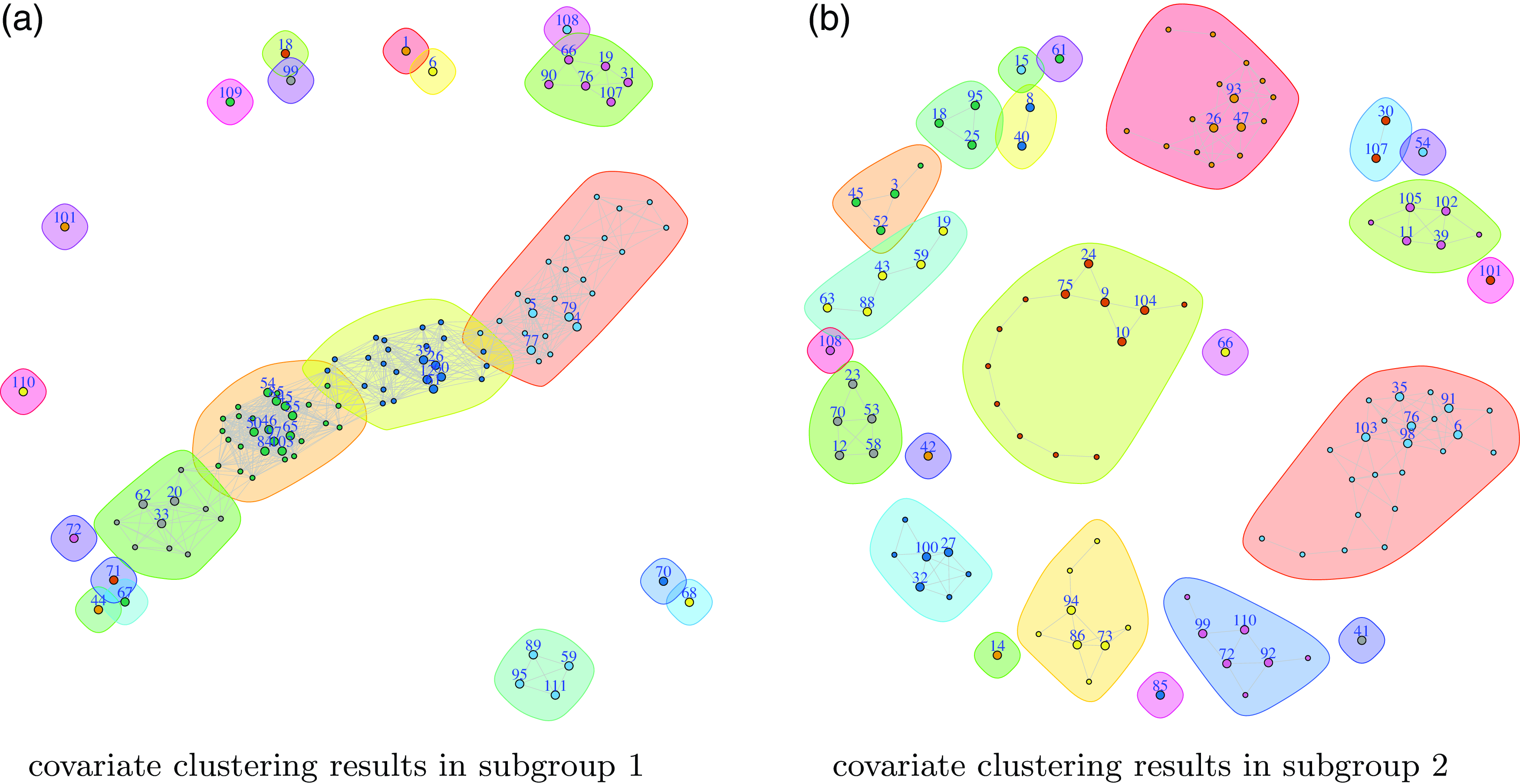
of subgroup 2, suggesting that most individuals have low healthcare costs. Figure 6 illustrates the clustering results of covariates in the two subgroups, represented by undirected and unweighted graphs (note that the distances between non-connected clusters do not indicate their similarity). Subgroup 1 predominantly groups the covariates into one main cluster in the middle and two minor clusters in the upper-right and lower-right regions, while the remaining covariates have unique effects that cannot be clustered. Subgroup 2, on the other hand, yields more distinct clusters, enabling better differentiation of the covariates’ effects, consistent with the prior similarity analysis. The model clusters most covariates in subgroup 1 (low-cost group), while fine-tuning the clustering effects on subgroup 2 (high-cost group). Furthermore, the utilization of colored backgrounds provides a more nuanced representation of clustering outcomes, where community formation is determined by the edge betweenness of each vertex (Girvan and Newman, Reference Girvan and Newman2002).
Diabetes expense dataset: the density function of cost data (
 $/10,000$
) for two subgroups when the covariates are chosen to be the median of the sample.

Clustering results of the proposed model: the vertex is a covariate, the edge is an association between two covariates, and the covariates can be grouped into a single cluster if a connected path exists between them; the colored background depicts a covariate’s “community” with finer granularity than the “cluster”.

We further identify and compile a list of significant covariates for large communities, enabling exploration of their internal relationships. For instance, the largest cluster of subgroup 1 can be subdivided into four communities, with one of them containing “V4,”“V5,” “V77,” and “V79,” which relate to fundamental knowledge and the detrimental effects of smoking on diabetes patients.Footnote 2 In statement “V4,” it is suggested that emotional stress can impact blood sugar levels in individuals with diabetes. Statement “V5” asserts that blood sugar levels may not necessarily increase the likelihood of developing complications associated with diabetes. Statement “V77” suggests that smoking can significantly increase the risk of severe diabetic foot amputation in individuals with diabetes. Statement “V79” notes that the combination of smoking and diabetes can lead to an increased risk of stroke. While we have only conducted basic analyses based on the covariates’ network structure, using more semantic methods in the future can improve the definition of the similarity matrix and provide more comprehensive insights into patients’ diabetes self-perception.
6. Conclusion
This paper proposes a framework for implementing covariate clustering in mixture regression models, which can identify and analyze the effects of covariates on heterogeneous population subgroups. The proposed framework incorporates a novel regularization term and uses the EM-ADMM algorithm to solve the complex optimization problem, thereby exploring the potential network graph of the covariates and conducting feature selection. Moreover, it can be regarded as an extension of GLMs with a convex covariate clustering procedure.
The empirical study aims to investigate the use of self-perception data related to diabetes, as measured through individual questionnaires, in predictive modeling. This study contributes to research in several ways. First, we employ eight feature selection and clustering algorithms (M1–M8) based on both non-mixture and mixture models to cluster a questionnaire dataset consisting of 111 variables. We evaluate these models in terms of goodness of fit, predictive accuracy, and discriminative ability. Mixture models, particularly those employing subgroup analysis with clustering methods, demonstrate the ability to effectively capture most of the sample values and provide advantages in point estimation. This is beneficial for the analysis of increasingly larger, multidimensional, and complex healthcare databases. We also emphasize the importance of considering the trade-off between predictive accuracy and risk discrimination when selecting the most suitable modeling approach. Second, our graph analysis of the clustered questionnaire data reveals the intricate interplay of factors affecting the management and potential complications of diabetes within different subgroups. This underscores the need for a holistic approach to treatment and risk reduction tailored to individuals in these distinct subgroups who have diabetes. Additionally, utilising self-perception data may provide information to the insurance company allowing for the design of medical insurance products that cover the risk of chronic diseases. This information, in turn, enables the provision of medical counselling services to insured individuals for the early intervention in the treatment of chronic diseases. To assess the robustness of the proposed algorithm, we conduct several simulation experiments and analyze another dataset related to short-term health insurance in China.
However, this paper has several limitations worth noting. First, the definition of the similarity matrix significantly impacts the results of covariate clustering and relies heavily on prior or expert knowledge. In our analysis, we only consider the similarity matrix by computing the cosine similarity of covariates, but incorporating natural language processing (NLP) approaches could enhance the definition of the similarity matrix and provide more comprehensive insights into patients’ diabetic self-perception. Second, this paper does not address the specific optimization of the execution speed of the algorithm, such as implementing parallel processing techniques. Future research could also explore expanding the range of distributions in mixture models and applying additional similarity penalties to covariates. For instance, replacing the Gamma distribution with a Poisson distribution for frequency predictions or a Tweedie distribution for aggregated loss predictions (including zero values) (Yang et al., Reference Yang, Qian and Zou2018), and incorporating penalty terms such as SCAD or MCP, could improve model performance. These modifications could enable our model to be applied in a wider range of scenarios, such as spatiotemporal data modeling, where covariate clustering is particularly useful for reducing data dimensionality or characterizing the correlation relationships among covariates.
Supplementary material
The supplementary material for this article can be found at https://doi.org/10.1017/asb.2025.13.
Acknowledgments
We are deeply grateful to the editor and the two anonymous reviewers for their constructive comments and suggestions, as well as to Prof. Peng Shi for his assistance in improving this article. Zhengxiao Li acknowledges the financial support from the National Natural Science Foundation of China (Grant No. 72271056) and “the Fundamental Research Funds for the Central Universities” in UIBE (Grant No. CXTD13-02). Yifan Huang acknowledges the financial support from the National Natural Science Foundation of China (Grant No. 72201062) and the National Social Science Fund of China (Grant No. 22ATJ005).
Competing interests
The authors declare no competing interests.