NOMENCLATURE
- C D
-
drag coefficient
- C L
-
lift coefficient
- C p
-
pressure coefficient
- D
-
diameter of hole, m
- δC D
-
drag coefficient increment
- δC L
-
lift coefficient increment
- δt
-
interframe time, s
- J
-
momentum flux ratio
- L i
-
linear dimension of interrogation area, m
- R
-
radius of hole, m
- V f
-
tunnel freestream velocity, m/s
- V R
-
velocity ratio (V jet /V f )
- V x
-
velocity in x direction, m/s
- V y
-
velocity in y direction, m/s
- V z
-
velocity in z direction, m/s
- x/c
-
normalised distance in the chordwise direction
- y/c
-
normalised distance in the spanwise direction
- z/c
-
normalised distance in the vertical direction
Acronyms
- CVP
-
Counter-Rotating Vortex Pair
- HSV
-
Horse Shoe Vortex
- JICF
-
Jets in Cross-Flow
- Nd:YAG
-
Neodymium-doped: Yttrium Aluminium Garnet
- PIV
-
Particle Image Velocimetry
Greek Symbol
- α
-
Incidence angle, °
- Δx
-
displacement vector in image domain, m
- ρ
-
density, kg/m3
1.0 INTRODUCTION
It is increasingly common for unmanned aerial vehicles to fly in areas where the risk of damage is high. Survivability is a key consideration when designing aircraft that fly in such places. It is important to consider the aerodynamic effects of battle damage to a wing, beyond structural integrity, as increased drag due to battle damage will result in increased fuel burn. As far back as the 1960s, studies were being undertaken to determine the effects of battle damage on the aerodynamic capabilities of a wing or aircraft. In 1968, Hayes(Reference Hayes1) simulated damage on a swept-wing model by removing wing panels. Although this early work was crude in its approach, it provided a basic understanding of the effects of battle damage. It was not until the 1990s that a systematic technique to test battle damage was developed. Irwin(Reference Irwin2) used simulated damage with uniform hole shapes and sizes in relation to chord length. Irwin conducted studies on the modelling of battle damage and presented data relating to damage occurrence, damage processes and damage shape. A summary of this can be found in Irwin and Render(Reference Irwin and Render3), while a full description can be found in Irwin(Reference Irwin2). As well as Irwin’s work, investigations have been carried out into the effects of damage holes with different shapes (Mani and Render)(Reference Mani and Render4), damage from live fire (Robinson and Leishman)(Reference Robinson and Leishman5) and three-dimensional tests using wings of finite span (Samaad-Suhaeb)(Reference Samaad-Suhaeb6) and (Djellal)(Reference Djellal and Ouibrahim7). The technique developed by Irwin is now the most commonly used method to test battle damage. Simulated damage is used because it makes use of regular shapes (e.g., circles) with sizes in relation to the chord length of the wing. This technique is preferred over live fire damage because it makes the experimental variables easier to control; using live fire to produce damage can cause random shapes and sizes that differ from test to test. However, Irwin’s investigations showed that a circular hole is the most common shape approximation of damage. As a consequence, much of the work subsequent to Irwin, including the current study, used circular holes. Although this is a reasonably established practice, the damage of a wing component in battle remains a stochastic phenomenon. This study does not attempt to progress techniques for modelling the variability of the damage shape in single strike events but adopts the hypothesis of a circular hole and explores in detail its aerodynamic performance consequence.
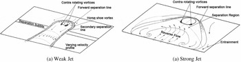
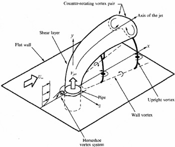
Irwin identified the main flow features produced by a single simulated damage hole and characterised them as a weak jet and a strong jet (see Fig. 1, as reported in Irwin and Render(Reference Irwin and Render3)), a third case occurs in transition between a weak and a strong jet which can display features of both. It was concluded that battle damage reduces lift, increases drag and changes the pitching moment. The prominent features of a weak jet are the narrow reverse flow region, as shown in Fig. 1(a) where the jet is attached to the wing surface towards the trailing edge, and the lack of freestream penetration by the jet. The jet and the Horse-Shoe Vortex (HSV) remain close to the upper surface of the wing. Different flow features can be seen for a strong jet case; the jet penetrates the freestream and creates a larger reverse flow region in both the vertical and spanwise directions. The HSV is larger and does not remain attached to the wing surface. Although Irwin(Reference Irwin2) did not measure the mainstream flow he theorised, from surface flow visualisation, that the surface pressure distributions and flow features for battle damage had similarities with Jets In Cross-Flow (JICF). Figure 2 shows the flow features of a typical flat plate JICF; the formation of the HSV can be seen just in front of the jet. The jet trajectory is affected by the cross-flow, bending it in the cross-flow direction and the Counter-Rotating Vortex Pair (CVP) is seen in the jet. The features of JICF seen in Fig. 2 are described in more detail later in this section.
Sketch of the key flow features of a weak jet and a strong jet from a single simulated battle damage hole, from Irwin and Render(Reference Irwin and Render3).

Vortex system from typical flat plate in cross-flow, from Kelso et al(Reference Kelso, Lim and Perry8).

Previous work on battle damage has concentrated on balance measurements to determine lift and drag increments (e.g., Pickhaver and Render(Reference Pickhaver and Render9)) with only limited flowfield information available from surface flow visualisation, as in Irwin and Render(Reference Irwin and Render10). This has provided a limited understanding of the flowfield and flow mechanisms, hence the need for more in-depth studies involving PIV. CFD simulations were performed by Yang et al(Reference Yang, Samaad-Suhaeb and Render11) and Saeedi et al(Reference Saeedi, Ajalli and Mani12) on a solid model (no cavity), but were not validated, hence the need for more relevant CFD predictions on the current wing model. Irwin(Reference Irwin2) performed experiments to test the effects of an internal cavity and concluded that it had only a small effect on the external flow and the lift and drag performance, but there is limited flowfield evidence to support this assertion. Bou-Mosleh and Patel(Reference Bou-Mosleh and Patel13) performed CFD simulations on multiple damage cases, including a small box cavity. However, little flowfield information inside the cavity is provided, hence the need for further investigation. Even though the fundamental external flow features produced by battle damage flow have been documented, they are not understood in great detail.
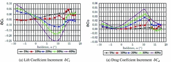
Render and Pickhaver(Reference Render and Pickhaver14) extended Irwin’s studies and investigated the influence of battle damage on a NASA LS(1)-0417MOD aerofoil at a Reynolds number of 500,000. Figure 3 shows the force coefficient increment data (force coefficient of damaged wing minus force coefficient of undamaged wing) for simulated battle damage with holes of varying size, all located at half-chord. For hole sizes of 5% and 10% chord, there is little difference in the aerodynamic performance until the high incidence angles. However, the effects of the larger holes are more significant with large reductions in lift and increases in drag. Below the zero lift angle the jet flow direction is reversed leading to a reduction in negative lift. In all cases, both lift and drag increments worsen with incidence. Beyond α = 10° the trend reverses due to the large amounts of separation on the upper surface of the wing(Reference Render and Pickhaver14).
Force increments for damage holes located at mid-chord, from Render and Pickhaver(Reference Render and Pickhaver14).

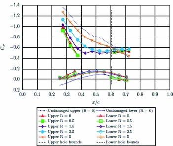
Figure 4 shows the surface pressure distribution over the upper and lower surfaces of the damaged aerofoil with a damage hole of 20%c diameter located at mid-chord, along with the undamaged wing surface pressure distribution. The hole bounds are shown as vertical dashed lines at 0.4x/c and 0.6x/c. On the upper surface there is an adverse pressure gradient in front of the hole along its centreline and at R = 0.5 off the centrelineFootnote ‡ . Compared to the undamaged case, the pressure coefficient (C p ) and the adverse pressure gradient both increase with the presence of the damage hole. The increase in C p indicates a reduced velocity on the surface of the wing and the increase in pressure gradient can be attributed to the blockage effects of the jet, as found by Doligalski et al(Reference Doligalski, Smith and Walker15). The pressure gradient behind the hole is small for all spanwise locations, even though a pressure gradient was present for the undamaged wing, indicating that there is little change in velocity in this region.
Surface pressure data for the damaged wing at 8°, from Render and Pickhaver(Reference Render and Pickhaver14). Each line denotes a different spanwise location from the centre of the damage hole.

From previous studies of battle damaged wings, it is clear that a jet of air passes through the wing and out into the freestream flow above the wing, very similar to classical JICF. Mahesh(Reference Mahesh16) defines the term ‘Jet in Cross-flow’ as referring to a jet of fluid that exits an orifice to interact with the surrounding fluid that is flowing across the orifice. By this simple definition, the problem being described in this paper can be thought of as a JICF. Important parameters in the study of JICF are jet velocity ratio, V R (Equation (1)), where V jet is the mean velocity across the hole exit and V f is the freestream (or cross-flow) velocity, and momentum flux ratio, J (Equation (2)), where ρ jet and ρ∞ are the density of the jet fluid and of the cross-flow fluid, respectively. Since this study was performed using air as a fluid with no density changes, ρ is constant and J is equal to V 2 R .
 $$\begin{equation}
V_R = (V_{jet} / V_f ),
\end{equation}$$\\
 $$\begin{equation}
J = \rho _{jet} V_{jet}^2/ \rho _f V_f^2
\end{equation}$$
In classic JICF, V R and J are often easier to calculate due to the experimental arrangements. In most cases, the jet will be issuing from a recessed pipe, driven by a metered air supply and passing through the full area of the pipe. With this set-up, it can be assumed that the change in mass flow across the diameter of the pipe is small, making measurements of the jet mass flow rate simple. In the case of battle damage, the jet is not driven by an external source, such as a compressed air reservoir, but exists due to the pressure difference between the pressure and suction surfaces of the aerofoil. There is also a cavity in the centre of the wing, meaning the jet enters and leaves a large space rather than passing through a solid pipe. Hence, it is not easy to measure V R for a battle damaged wing.
Key features of JICF are the CVP and HSV, as mentioned previously. The exact nature of the flow physics behind CVP formation is disputed, but the general consensus is that the CVP formation occurs due to the modification of the jet vorticity by the cross-flow, a process that happens in the near field (see Kelso et al(Reference Kelso, Lim and Perry8), Cortelezzi and Karagozian(Reference Cortelezzi and Karagozian17) and Marzouk and Ghoniem.(Reference Marzouk and Ghoniem18)). Gopalan et al(Reference Gopalan, Abraham and Katz19) state that at velocity ratios >2, the higher jet momentum resists the cross-flow and bends far away from the wall. The jet vorticity, although distorted by the cross-flow, is carried away from the wall by the momentum and remains confined to the jet (the increased clearance between the jet and the wall allows the jet to keep its vorticity). When this is the case, the jet vorticity aligns itself with the streamwise direction, forming the CVP.
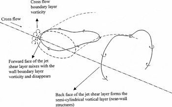
The flow features at velocity ratios <2 differ from those explained above. The so-called semi-cylindrical vorticity layer, a sketch of which can be seen in Fig. 5, exists due to the forward and inner boundaries of the jet experiencing different conditions as the jet leaves the hole. The back side of the jet shear layer is protected from the incoming cross-flow and is exposed to slow moving fluid, mostly from the reverse flow region. Conversely, the forward face is exposed to the incoming cross-flow. On the forward side of the hole, the vorticity of the cross-flow boundary layer and the vorticity of the jet have opposite signs. Gopalan et al(Reference Gopalan, Abraham and Katz19) and Mahesh(Reference Mahesh16) conclude that this interaction, along with the cross-flow moving over the jet due to the low jet momentum, causes the disappearance of jet vorticity at the forward side (the cross-flow vorticity effectively overwhelms the jet vorticity). The result is the effective shedding of vorticity at the back and the formation of the semi-cylindrical vortical shell with a ‘dead zone’ at the back side of the jet. The cause of the jet vortex ring ‘stretching’ at the back of the hole (seen in Fig. 5) is due to the significant differences in vertical velocity components between the front and back of the jet.
Representation of the semi-cylindrical vortical layer behind the jet at low velocity ratios (V R < 2), from Gopalan et al(Reference Gopalan, Abraham and Katz19).

It was shown by Almond et al(Reference Almond, Render and Walker20) that, with a battle damaged wing, the jet does not exit the full area of the hole, but the jet vertical velocity cross-section is biased towards the rear. The velocity ratio was also found to be low (<0.3). Gopalan et al(Reference Gopalan, Abraham and Katz19) classify a low velocity ratio (V R ) as <2; however, they performed experiments down to V R = 0.5. For comparison, a battle damaged wing showing ‘strong’ characteristics (i.e., large effects on lift/drag performance and large spanwise effects seen in flow visualisation studies) can have a velocity ratio as low as 0.22, increasing to around 0.3 at higher incidence angles(Reference Almond, Render and Walker20). This suggests that even at high incidence angles, the flow characteristics of the jet are of the weak jet type, using the JICF nomenclature, even though large effects can be seen in the aerodynamic performance and on the surface flow. Gopalan et al(Reference Gopalan, Abraham and Katz19) also observe the jet only exiting a small portion of the hole towards the rear and describe this mechanism as ‘squeezing’ of the jet. Ki-Young(Reference Ki-Young21) also concluded that the flow structure created by battle damage on a wing at low incidence angles shows agreement with the work from Gopalan et al(Reference Gopalan, Abraham and Katz19) and Mahesh(Reference Mahesh16).
The aim of the current paper is to further understand the flow structures created by simulated battle damage and relate them to accepted theory on JICF, whilst identifying similarities and differences and explaining why these occur. The flow characteristics will be related to the force coefficient increments to try and explain why large differences are seen through the incidence range. In this work, the battle damage model is limited to a circular hole, consistent with previous studies (Irwin(Reference Irwin2) and Pickaver(Reference Pickhaver22)). It is acknowledged that a broader investigation on the shape and location effects of battle damage, including multiple holes and uneven hole edges (petalling), is required for improving the survival rate from individual damage events.
2.0 METHODOLOGY
2.1 PIV Experiments
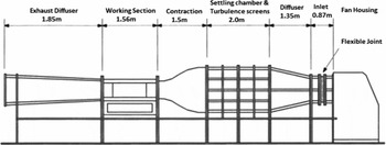
The tests were conducted in the Loughborough University Low Turbulence Wind Tunnel. The wind tunnel is of open return design with a closed working section measuring 0.45 m × 0.45 m. Typical inlet turbulence intensity is approximately 0.1%. For convenience, the model was attached to an under-floor force balance, although no balance data will be presented in the present study. The tests were performed at a wind speed of 37 m/s, which gave a Reynolds number of 500,000 with a model of 200 mm chord. A schematic diagram of the wind-tunnel facility is shown in Fig. 6.
Schematic of Loughborough University Low Turbulence Wind Tunnel(Reference Render and Pickhaver14).

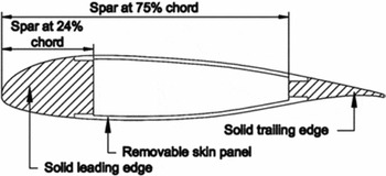
The wing model used a NASA LS(1)-0417MOD aerofoil. This profile was chosen because of its close similarity to the wing profiles of existing reconnaissance unmanned aerial vehicles. To represent typical construction of aircraft the wing-section model was of hollow construction and used removable composite skin panels. Damage was applied to the panels using a laser cutter and the panels were fixed using counter-sunk screws so that they sat flush with the wing surface. A spanwise cross-section of the wing model is shown in Fig. 7. Two damage cases were chosen for this work, each with a single hole located at half chord. The first was a hole of 20% chord diameter. This was chosen because it provides a typically survivable damage case that produces both a weak and a strong jet over the incidence range tested. Secondly, a hole of 40% chord length in diameter was tested for use as a comparison, as this is considered the upper limit of survivability from a structural perspective.
Sketch of thin-walled wing cross-section(Reference Render and Pickhaver14).

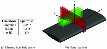
A LaVision two component PIV system was used in three streamwise planes (hereafter referred to as chordwise) and three spanwise planes, Fig. 8 shows the locations of these planes. Two separate set-up configurations were used for each plane direction. The chordwise planes required the camera to be located outside the wind tunnel, at 90° to the wing cross-section. The spanwise planes required a more complex set-up, with the camera located inside the wind tunnel downstream of the working section. The camera was located in a perspex box to protect it from the wind and from seeding fluid; the camera was mechanically decoupled from the box to ensure that no vibrations were transferred from the box to the camera. This was done to improve the image quality.
Location of chordwise (red) and spanwise (green) PIV planes and reference coordinate system.

The light sheet for the PIV was produced by a 200-mJ double-pulsed Nd:YAG laser, located above the working section of the wind tunnel on a traverse mechanism. The laser emits a circular beam of 4 mm diameter, which, when focused through a cylindrical lens, gave a light sheet of approximately 1 mm thickness at the measurement plane. A single Imager LX 8M CCD camera with a resolution of 3312 × 2488 pixels was used to record the PIV images using a 105-mm focal length Nikon lens with an aperture value of 1/5.6. The camera and laser were controlled by a LaVision external Programmable Timing Unit (synchronizer), which sets the trigger rate at 8.5 Hz. The typical time between images within a pair (interframe time or δt) was 30–40 μs; this was optimised for each set-up position. The flow was seeded with 1–2 μm particles produced by a LaVision aerosol generator at 4 bar using olive oil as the seeding fluid. It was shown by Hollis(Reference Hollis23) that oil particles of 2 μm faithfully followed the flow in air for accelerations greater than seen in this experiment, giving an acceptable particle velocity lag at the worst-case scenario.
The system was calibrated in each measurement plane using a two-dimensional calibration plate. The markings on the plate represented a known dimension in x and y, allowing the software to perform a spatial calibration for use in the velocity measurements. To verify that the PIV and wind-tunnel settings were appropriate, 50 image pairs were taken over a range of δt values and processed to check for data quality and peak locking. The particle image diameter was between 1 and 2 pixels (the apparent size of the particle based on the scattered light entering the camera lens), meaning pixel biasing effects were within acceptable limits in regard to the quality of the measured flow patterns and flow statistics(Reference Adrian and Westerweel24). A total of 1,000 image pairs were taken for each incidence angle and processed using LaVision’s DaVis 8.0 software. An additional test taking 2,000 images showed no significant improvement in the statistical accuracy of the PIV data(Reference Hollis23).
The processing of images was a four-step procedure. First, a background image was removed by applying a time filter; this helps reduce any effects from background light or any constant sources of light that may be present in the image (such as light reflections). A geometric mask was then applied to the images to discard any parts that were taken up by the model, as the data in this region would be noise. The third step was vector calculation, which was performed using a multi-pass technique. The chordwise and spanwise planes required different parameters because the flowfield was very different. In both cases, five passes were done in total, two at a larger window size (64 × 64 pixels) and three at a smaller window size (32 × 32 for the chordwise planes and 24 × 24 for the spanwise planes). The smaller window size in the spanwise planes was possible due to the lower δt values used because of the high amounts of out of plane motion. A window offset correlation was used in the multi-pass processing to improve the peak detectability for the displacement peak by reducing the in-plane loss of correlation. This allowed the use of smaller window sizes to increase the spatial resolution. The number of vectors in the final vector field was approximately 14,000. The final step of the processing was taking an average vector field from the 1,000 instantaneous image pairs.
The accuracy was optimised for the jet and the reverse flow region, with the trade-off being a less than optimal arrangement in the freestream. The average particle displacement in the reverse flow region is 7.4 pixels, conforming to the design rule defined by Adrian and Westerweel(Reference Adrian and Westerweel24) shown in Equation (3) by which the displacement vector |Δx| ought to be less than a quarter of the linear dimension of the final interrogation area, LI:
 $$\begin{equation}
\vert \Delta x \vert < \frac{1}{4} \text{L}_{\text{I}}
\end{equation}$$
In the freestream, the value was much higher at 22 pixels. Although this value was higher than the optimum, the flow is nominally consistent and laminar in its passage through the area of interest, meaning the software easily calculated the velocity, helped by the multi-pass processing technique. In the freestream, the instantaneous velocity fields showed over 99.8% first-choice vectors, higher than the turbulent reverse flow region, which produced around 90% first-choice vectors. The remaining data were removed during processing due to it being more than 2 standard deviations away from neighbouring vectors. This technique reduces spurious vectors and improves the average vector field.
The surface flow visualisation photographs taken from Pickhaver(Reference Pickhaver22) were used during the analysis of the results and these were obtained using a mixture of titanium dioxide powder, linseed oil and paraffin. The mixture was applied to the upper surface of the model using spanwise strokes of a paint brush. The tunnel was then run at the normal test speed of 37 m/s, and the flow patterns were photographed from above the working section. The wind tunnel was left running during this process to ensure the visible flow patterns were those caused by the airflow and not from gravity after the airflow was turned off.
2.2 Computational Fluid Dynamics
Standard CFD techniques were employed for the numerical work with RANS predictions generated using the commercial CFD package Star-CCM+. The entire working section of the wind tunnel was modelled to ensure similarity with the experiment. A velocity inlet was used to replicate the measured wind-tunnel inlet conditions. An unstructured polyhedral mesh was used along with volumetric controls to increase mesh density in important regions (e.g., the wing cavity, jet and wake region). Prism layers were also used to increase the near wall mesh density and ensure y+ values close to unity in order to resolve the boundary layers. Although not reported here, a mesh dependency study was conducted varying both the global cell density and the local cell density in the cavity and in the wake region. For the final mesh, the overall cell count was close to 2.8 m cells with approximately 50 cells across the hole. Increasing the overall cell count close to 5 m did not notably alter the CFD predictions. Importantly, the 2.8 m cell mesh enabled incompressible RANS solutions to be generated on a high-performance desktop PC within reasonable timescales. The solutions were generated using a segregated solver with second-order upwind differencing. Turbulence was modelled using the two-equation realisable k-ε model in conjunction with a low y+ near wall approach. A k-ω SST model was also examined, however, it did not perform as well as the k-ε model with regards to predicting the shape of the jet.
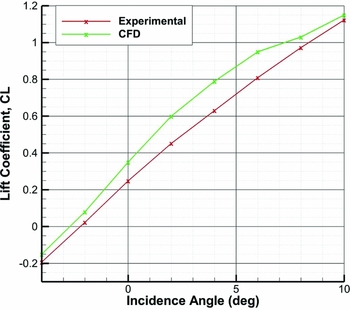
To reiterate, the main aim of the CFD was to support the PIV measurements in and around the wing cavity where it was not possible to obtain experimental data. In order for the CFD to be used to examine the cavity flow, it must first be validated against the external flowfield measured using PIV. Figure 16 shows colour iso-levels of velocity magnitude on the mid-plane through the hole at an incidence of 8°. Details of the flowfield will be discussed later, but it is clear from Fig. 16 that the PIV and CFD data are in relatively good agreement. There are subtle differences, but the agreement is more than sufficient to give confidence in the predicted cavity flow. In terms of overall performance, Fig. 9 shows that the CFD simulations over-predicted the absolute values of lift to those measured experimentally; however, the trends were accurately reproduced.
Comparison of lift coefficient obtained experimentally and lift coefficient from the (CFD) simulations.

3.0 RESULTS AND ANALYSIS
PIV data have been used to identify several features of the flowfield produced by simulated battle damage(Reference Almond, Render and Walker20). More specifically, it has been used to describe the flow features on the upper surface of a wing, with particular interest to the areas above and behind the hole. The external flow features created by a 20%c and a 40%c hole will be described using PIV and CFD data. Then, because the CFD showed good agreement with the external flow features, it will be used to describe the flow structures inside the cavity, where experimental data are lacking.
3.1 20% Chord Damage Hole
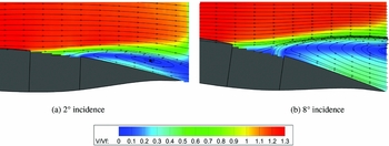
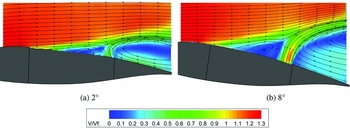
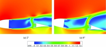
The chordwise planes provide a perspective of the flow in the direction of the freestream. Figure 10 shows the PIV data along the centreline of the hole at 2° and 8° incidence. All velocities have been normalised by the freestream velocity, V f . A jet can be seen exiting through the hole on the suction side of the wing. The bulk of the jet mass flow exits through the rear of the hole in both cases, forming a reverse flow region behind the jet shear layer above it. The incoming cross-flow merges with the jet as it becomes aligned to the cross-flow direction. The maximum freestream penetration is approximately 0.5 hole diameters for the 2° case and 1 hole diameter for the 8° case. This was estimated by measuring the distance from the wing-suction surface to the jet shear-layer boundary, 1.5 hole diameters downstream of the hole trailing edge. The size of the jet is approximately 1/8D in this plane at 8°, determined by measuring the vertical core of the jet at the same chordwise location.
Colour iso-levels of in-plane velocity magnitude and streamlines from PIV on hole centreline.

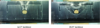
As was noted by Almond et al(Reference Almond, Render and Walker20), the bulk of the jet mass flow exits through the rear of the hole, with a velocity ratio of around 0.13 and 0.3 for the 2° and 8° cases, respectively, measured in the centre of the jet. This velocity ratio is low compared with the majority of JICF applications and would be classed as a weak case. Looking at the very back of the hole, the reverse flow can be seen impinging on the jet. The 8° incidence case creates a more vertical trajectory than the 2° incidence case in this impingement zone. The flow visualisation images shown in Fig. 11 highlight some of the prominent flow features close to the surface. The reverse flow region seen in the PIV can also be seen here, travelling from the wing trailing edge to the back of the hole. The difference between 2° and 8° is a larger spanwise effect; the wake region at the wing trailing edge growing from around 1.5 hole diameters wide at 2° to 5 hole diameters at 8°. The increase in affected surface area contributes to the increased aerodynamic losses at higher incidence angles. A Horse-Shoe Vortex is seen to form ahead of the jet in both cases, before travelling downstream and surrounding the wake region created by the jet.
Surface flow visualisation images of the wing upper surface, from Pickhaver(Reference Pickhaver22). Freestream flow direction from bottom to top.

The flow visualisation shows a significant change in flow behaviour between 2° and 8°, as mentioned in Section 1. The behaviour and flow mechanisms between low incidence angles and high incidence angles were thought to be very different(Reference Gopalan, Abraham and Katz19). However, the change is less severe in the PIV data. The data suggest that the same features exist in both cases, with an increase in the jet strength as the incidence angle is increased. PIV tests have been performed at all angles between 2° and 8°, and no distinct switch in flow pattern was seen. When comparing the velocity ratio found in Almond et al(Reference Almond, Render and Walker20) with JICF literature, all incidence angles from the battle damage studies should produce ‘weak’ jet features. However, large effects on aerodynamic performance are seen throughout the incidence range, particularly above 2° incidence. More PIV data must be considered before an explanation to this behaviour can be presented.
Figure 12 shows the in-plane velocity magnitude iso-levels for the 8° case at y = 0.25D and y = 0.5D; y = 0.5D being the edge of the hole. It can be seen that compared to Fig. 10(b), the height of the reverse flow region reduces and the jet shear layer is visibly thinner. The freestream penetration is reduced from 1D on the centreline to 0.9D and 0.7D at locations of 0.25D and 0.5D, respectively (measured 1.5D downstream of the hole), indicating that the jet strength is highest along the centre of the hole and reduces towards the edge. For completeness, the maximum velocity ratios at the y = 0.25D and y = 0.5D locations are 0.19 and 0.1, respectively, compared with 0.3 on the centreline.
Colour iso-levels of normalised in-plane velocity magnitude at y = 0.25D and y = 0.5D, both at 8°. Vertical lines show the approximate local hole cross-sections.

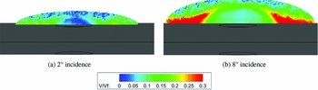
Figure 13 shows PIV data in a spanwise plane located 0.5 hole diameters downstream of the hole trailing edge. As shown by the figure legend, the velocity magnitudes are much smaller in this plane, as the majority of the flow motion is out of plane (coming towards the reader). The wake region for both incidence angles is contained within a semi-elliptical region. Above this area, the PIV images produce high amounts of noise due to the flow being entirely out of plane, therefore this portion of the measurement plane has been omitted from the figure. The highest in-plane velocity magnitudes in both cases are outboard of the hole edges, with the flow moving outwards in the spanwise direction. The velocity above the hole itself is low. The width of the data plane is 3.4D for 2° incidence and 4.2D for 8°, which is the width of the wake at this location.
Colour iso-levels of in-plane normalised velocity magnitude on the spanwise plane 1D downstream of the hole centre.

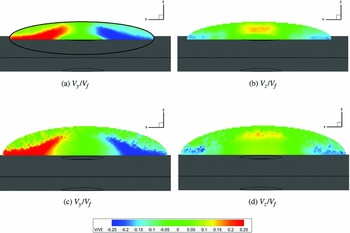
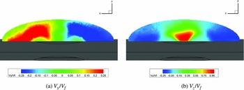
A more detailed picture of the flow can be obtained by separating the contributions from the y (spanwise) and z (vertical) velocity components, which allows specific features to be identified. Figure 14 shows the iso-contours of y and z velocity components from PIV at a spanwise plane located at the trailing edge of the hole. The y velocity (Fig. 14(a)) shows an outflow of jet fluid in the spanwise direction. This can also be seen in the surface flow visualisation (Fig. 11) where the surface flow can be seen travelling outwards towards the HSV. This explains the increasing width of the affected surface area at higher incidence angles. The z velocity is lower in magnitude which is due to the jet aligning itself with the cross-flow and therefore not having a large vertical component of velocity at this location.
Spanwise PIV data showing normalised y and z velocity at the hole trailing edge (a) and (b) and 1D downstream of hole centre (c) at (d) at 8° incidence.

A feature noticeable from the spanwise planes is the semi-elliptical shape of the wake region, as highlighted in black in Fig. 14(a). This trend also matches the features noted in the chordwise planes of reducing reverse flow region height and reducing penetration as the chordwise plane is moved away from the hole centre. The jet size, estimated by looking at the z velocity at the hole trailing edge and spanwise planes over the jet (not shown) is approximately 1/4D. This was estimated by blanking the z = 0 iso-level, thus defining the edges of the jet. This means the jet shape can be approximated as an ellipse (1/8D wide by 1/4D deep), meaning the jet occupies approximately 0.125 of the hole area.
From the PIV data, it can be seen that the size of the jet increases as the incidence angle is increased. This can be seen best in Fig. 10 over the jet opening towards the rear, where the core of the jet is more visible in the 8° case. This introduces some complexity in the way the jet can be idealised, compared to a JICF. Specifically, the jet is thought of as an eliptical solid protruding into the flow, then as incidence angle is increased, the size of the ellipse is increased. If the jet size is larger, then a larger obstruction is presented to the flow, hence a larger HSV and wake region will form. This is further complicated by an increased adverse pressure gradient on the wing surface at the higher incidence angle (Fig. 4), making the cross-flow more susceptible to separation. The adverse pressure gradient on the wing has a magnified effect on the wake compared with the cross-flow (or freestream); the low momentum wake fluid is less able to overcome the adverse pressure gradient and therefore slows, spreads more and is more prone to separation.
The effects of the jet can now be considered. It is known that the velocity of the jet increases, albeit not by a large magnitude, by increasing the angle of incidence. This produces more freestream penetration, which in turn produces a larger wake region in the vertical plane. Combining with the adverse gradient effect, this produces a larger wake region as the incidence angle is increased, with the largest change in wake region size being in the spanwise direction. This increase creates a larger recirculation region, which causes the jet to expand spanwise, as seen in the PIV iso-levels of Fig. 13. Further, the increasing reduction in lift and increase in drag reported in Section 1 can be attributed to the increase in wing area that is affected by the wake region.
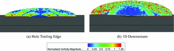
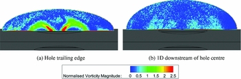
From the literature on JICF, the spanwise plane should display the counter-rotating vortex pair in the jet as a prominent feature of the flow. However, this is not the case, as shown in Fig. 15. At the trailing edge of the hole (Fig. 15(a)), the normalised x-vorticity can be seen emanating from two points in line with the edges of the hole. These are not the CVP, but x-vorticity produced by the sideways expansion of the jet (seen in Fig. 14(a)). Figure 15(b) shows x-vorticity on the spanwise plane 0.5D downstream of the hole trailing edge, indicating that this vorticity component is significantly reduced. Even though the jet has a better alignment with the cross-flow (and hence the PIV plane) no characteristic kidney-shaped vortex pair can be seen. Indeed, it is difficult to even identify the jet in this second plane. Elevated levels of x-vorticity can be seen at the extremities of the shear layer that bounds the wake region, shown on the outer regions of the measurement plane. As seen in the chordwise planes, the shear layer thickens as it moves downstream, which is reflected in the increased spatial extent of the x-vorticity that delimits the extent of the shear layer in Fig. 15.
Colour iso-levels of normalised x-vorticity magnitude shown at two axial planes behind the hole trailing edge, 8° incidence. Vorticity normalised by V f /D.

Several references, including Kelso et al(Reference Kelso, Lim and Perry8), Moussa et al(Reference Moussa, Trischka and Eskinazi25) and Coelh and Hunt(Reference Coelho and Hunt26), have noted that the CVP form from the thin vortex sheet (or thin shear layer) which emanates from the pipe, combined with the initial acceleration of the jet fluid by the cross-flow. During the current tests, a hollow model has been used to represent the internal structure of a wing. For this reason, there is no ‘pipe’, hence no walls for a nozzle boundary layer to feed into the jet shear layer, and hence no vorticity to carry into the cross-flow. Further, any vorticity taken into the cross-flow would tend to dissipate rapidly due to its interaction with the cross-flow boundary layer because of the low velocity ratio. The low jet momentum means the cross-flow boundary layer moves over the top of the jet, keeping the jet close to the wall (or wing surface) and forming the semi-cylindrical vortical layer, as sketched in Fig. 5.
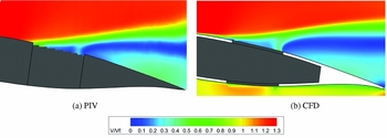
To help explain some of the external flow features, CFD was used to predict and examine the internal flow inside the cavity. However, before using CFD to study the flow structure inside the cavity, it was important to ensure the external flow features were predicted accurately by the numerical scheme. Figure 16 shows a comparison of the time-averaged in-plane velocity magnitude on the chordwise plane through the hole centreline between PIV and CFD at 8° incidence. In general, the CFD prediction shows a good qualitative agreement with the PIV measurements. The location and trajectory of the jet is well matched, as is the size and strength of the recirculating region. There are some subtle differences, such as the thickness of the jet core and the velocity magnitudes in the reverse flow region. However, the agreement is sufficiently good, so it is reasonable to use the CFD predictions to further examine the flow and in particular the effect of the wing cavity.
Colour iso-levels of in-plane velocity magnitude on the hole centreline providing a comparison of PIV and CFD external flow field data, 8° incidence.

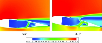
Figure 17 shows CFD predictions on the centreline plane taken through the hole, with the cavity flow visible. The flow coming into the cavity from the lower surface enters at a maximum velocity of approximately 0.6V f for the 2° case and 0.9V f for the 8° case and impacts the upper panel behind the hole. The bulk of the flow then travels rearwards to the back of the cavity, before moving down causing the flow to roll into a bound vortex; this vortex then extends spanwise in both directions. This feature will be referred to as the cavity vortex. The external ‘jet’ that can be seen in Figs 10(b) and 12 on the upper surface of the wing is not flow coming directly from the lower hole (i.e., straight through the wing), but more of an over-flow of the cavity.
Colour iso-levels of normalised velocity magnitude on a chordwise centreline CFD plane showing the cavity flow.

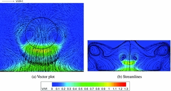
Figure 18 shows the flow inside the cavity on a horizontal plane located half way between the suction and the pressure surfaces. The colour iso-levels are levels of normalised velocity magnitude, while the vectors in Fig. 18(a) denote the in-plane velocity component. Figure 18(a) shows vectors of the flow in the vicinity of the hole, and Fig. 18(b) shows streamlines of the flow around the entire cavity. The internal jet, prior to contact with the upper surface of the wing, shows the highest y magnitude being located just downstream of the hole rear edge, as indicated by the yellow tone in Fig. 18(a). The vectors of Fig. 18(a) show that the in-plane chordwise velocity component is largest in this region of high velocity magnitude. Further downstream, the flow appears to be deflected spanwise by the rear wing spar. A vortex pair can be seen underneath the edge of the hole, in front of the jet, which corresponds with the location of a collection of flow visualisation fluid seen on the edge of the hole seen in Fig. 11(b). This internal vortex pair was first observed by Pickhaver(Reference Pickhaver22), when flow visualisation tests were performed on the inside of the panels. The vortex pair is created when the flow in the cavity vortex and flow recirculating back from the forward portion of the cavity impinges on the internal jet. Figure 18(b) shows the full cavity, revealing a second vortex pair in the forward corners. This vortex pair is larger; however, the flow in this region has lower velocity magnitude compared to the flow close to the hole. The cavity fluid then moves along the front surface of the cavity and moves backwards to form the jet.
Colour iso-levels of normalised velocity magnitude showing flow on a central plane inside the cavity, looking from above the wing with the freestream flow from top to bottom, 8° incidence.

The majority of the flow inside the cavity is low velocity recirculation, but the presence of the cavity is affecting the external flow. With no cavity (solid model), flow from the lower surface would travel straight through the hole (along the rear face), leading to a higher normalised jet velocity. However, as shown in Fig. 17, the internal jet is impacting the upper panel behind the hole and hence reducing the strength of the flow exiting through the upper surface. It is clear that the efflux from the hole is not a distinct jet but it is more like a spillage flow. This is one reason why the velocity ratio is low and the jet does not penetrate far into the freestream.
The flowfield for a 20% chord damage case can now be related to the change in the aerodynamic forces reported in Fig. 3. At 8° incidence, the lift coefficient increment is approximately three times bigger than at 2° incidence, and the same trend is observed for the drag. As the PIV and CFD data have shown, the differences between 2° and 8° are significant. In the vertical direction, it is likely that more flow enters the cavity from the lower surface. This increase causes a larger amount of spillage or outflow leading to a larger external jet. However, it is in the spanwise direction that the biggest changes in behaviour are observed. The outflow of jet fluid is stronger at higher incidence angles, leading to a larger wake that affects more of the wing surface area.
3.2 40% Chord Damage Hole
A 40% chord damage hole is now considered in comparison to the 20% chord damage hole case. This will help explain the importance of hole size in relation to the wing as well as hole size in relation to the cavity. As the cavity is kept the same size, its relative size in comparison to the hole is smaller. Figure 19 shows colour iso-levels of normalised velocity magnitude from PIV measurements on the hole centreline for a 40% chord damage hole. At first glance, the 40% chord damage hole case shows broadly the same flow features to the ones of the 20% chord damage hole but the jet is stronger and has a higher maximum velocity ratio of 0.5 at 2° and 1.2 at 8°. At both incidence angles, the maximum velocity ratio is four times higher than the equivalent test using a 20% chord damage hole. There is more freestream penetration, which in turn creates a larger reverse flow region and a larger wake in the vertical plane. Even though the freestream penetration is larger in Fig. 19 than in Fig. 10, when normalised by the hole diameter it is 0.4D at 2° and 1D at 8°.
Colour iso-levels of normalised velocity magnitude on a chordwise centreline PIV plane for a 40% chord damage hole.

The core of the jet is much better defined, particularly at 8° incidence, compared to the 20% chord damage hole case and can be easily distinguished from the flow features around it. The jet and cross-flow show much less merging close to the wing surface. This makes it easier to estimate the jet velocity ratio, as the jet is less affected by the upper surface cross-flow because it outflows through the suction side surface. At both incidence angles, there is a flow structure in front of the jet that does not occur in the 20% chord damage hole case. This structure is a low-velocity region created by the obstruction of the jet. It is larger at the higher incidence angle due to the larger obstruction, but in both cases flow appears to be moving between this region and the cavity.
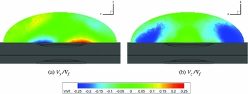
Figures 20 and 21 show the normalised y and z velocity components at two spanwise planes located respectively at the hole trailing edge and at 1 hole diameter downstream of hole centre. These planes extend 2.25D spanwise for the 8° test case. At the trailing-edge spanwise plane (Fig. 20), there is a large outflow of jet fluid in the spanwise direction surrounding the core of the jet located in the centre. The z velocity shows higher magnitudes (note the higher scale) in the jet, and lower negative z velocities in the wake region further outward compared to the 20% chord damage hole case shown in Fig. 14(b). At the rear spanwise plane (Fig. 21), low z velocity regions can be seen in the centre of the wake where the jet has aligned itself with the cross-flow, meaning that most of the flow is out of plane.
Colour iso-levels of normalised y and z velocity components measured by PIV at the hole trailing edge, 8° incidence.

Colour iso-levels of normalised y and z velocity components measured by PIV at the 1D downstream of hole centre location, 8° incidence.

Plots of the x-vorticity component can be seen in Fig. 22, at the same locations as the previous images, taken at 8° incidence. Much like the 20% chord damage hole case, x-vorticity can be seen emanating from the edge of the hole through the suction surface, moving in the spanwise direction. By the second plane 1D downstream of the hole centre, the x-vorticity magnitude has significantly reduced. The spanwise outflow from the hole appears to have flattened out over the wing suction surface, as shown by the two regions of positive x-vorticity (in red) either side of the hole centreline.
Colour iso-levels of normalised x-vorticity magnitude from PIV at two spanwise planes behind the hole, 8° incidence. Vorticity normalised by V f /D.

CFD has also been used to study the flow features inside the cavity with the 40% chord damage hole. The flow on the centreline chordwise plane is shown in Fig. 23. The pressure difference between the section and pressure sides causes ingress of flow through the pressure side hole, which bends upstream due to the blockage of the trailing-edge wing spar, forming a jet inside the cavity. Unlike with a 20% chord damage hole, there is much less suction surface wing skin at the back of the cavity for this jet flow to impact on; however, the trajectory of the jet does cause it to impact the panel at both incidence angles. At 8° incidence, the highest jet outflow velocity is predicted close to the suction side rear edge, in agreement with the PIV measurements of Fig. 19(b). Some of the flow passes straight through the wing, but the peak velocities in this internal jet can be seen where the jet is directed towards the suction surface rear skin, at 2°. Interestingly, the peak velocity of the jet at 2° occurs inside the cavity, mid-way between the lower and the upper surfaces. The cavity vortex is present at both incidence angles, but it is much smaller than that seen with a 20% chord damage hole. The 2° test shows a slightly forward trajectory of the jet as it leaves the hole, which agrees with the PIV data, caused by a deflection from the upper surface panel.
Colour iso-levels of normalised velocity magnitude on the chordwise centreline CFD plane showing the flow through the cavity, 8° incidence.

The cavity is having less of an effect on the external flow because the relative size of the remaining wing skin delimiting the cavity is smaller. The jet is behaving more like a jet passing through a solid model but is still only exiting a small percentage of the hole. The jet velocity ratio is still very low compared with that from a JICF.
As with the 20% chord damage hole, the flowfield can be related to the force coefficients. The 40% chord damage hole produces much larger changes in both the lift and drag coefficients than the 20% chord damage hole. This agrees with the PIV and CFD data that have shown that the 40% chord damage hole produces much stronger features. The wake region for the larger hole is taller, wider and extends further downstream over the wing, leading to large reductions in wing performance.
4.0 CONCLUSION
PIV and CFD have been used together to map the flowfield created by simulated battle damage to a two-dimensional hollow wing. The external flow features from two damage sizes have been examined and related to the corresponding features of JICF reported in literature. It has been shown that neither a 20%c nor a 40%c damage hole created conventional JICF features, such as the counter-rotating vortex pair, due to the very low velocity ratios and internal wing structure. An increase in wake size in the spanwise direction with increasing incidence has been attributed to the combined effects of an increasing jet blockage and of a strengthening adverse pressure gradient.
CFD has been used to understand the cavity flow inside a hollow damaged wing, which was previously assumed as having little effect on the external flow. This was found not to be the case, particularly for the 20% chord damage hole. The jet fluid entering the cavity from the lower surface does not pass through the wing unobstructed, but it impacts the upper surface before the bulk of the flow travels rearwards. The external jet is created by an over-flow from the cavity, explaining why the velocities in the external jet are low compared to the ones from a JICF exiting from a pipe. The cavity is much smaller relative to hole size for the 40%c hole case, enabling the flow at 8° to cross the wing section from the lower surface to the upper surfaces relatively unimpeded. However, the cavity still affects the jet trajectory at low incidence angles.
The flow features of both hole sizes have been related to the force coefficient increments and show good correspondence with the observed changes in the aerodynamic loads from force balance measurements. The increasing increments at higher incidence angles match well with the larger wakes and larger amount of affected wing surface area. Further, the wake region with the 40%c hole is significantly larger than with a 20%c hole confirming the balance data which shows larger performance losses occurring with the larger hole.
This investigation limited the battle damage analysis to round flush holes through a hollow wing. Given the stochastic nature of battle damage events and of the surviving structure, caution should be exerted in extrapolating general trends on all battle damaged structures and their aerodynamic performance from the current analysis.
ACKNOWLEDGEMENTS
The authors would like to express their thanks to David Cooper for the technical support he provided during the experiments.