



1. Introduction
Turbulent boundary layers are ubiquitous in various engineering applications, such as aerospace engineering, turbomachinery flows and naval engineering. The vast majority of turbulent boundary layers encountered in practical engineering scenarios are three-dimensional (3-D) and non-equilibrium. The three-dimensionality manifests as a misalignment between the primary flow direction and the pressure gradient (Schlichting & Gersten Reference Schlichting and Gersten2017). This misalignment induces a crossflow velocity perpendicular to the primary flow direction, significantly altering the characteristics of the shear stress distribution within the boundary layer. In the present study, the non-equilibrium effect is characterised by a local imbalance between turbulence production and dissipation (Devenport & Lowe Reference Devenport and Lowe2022), exhibiting a strong dependence on upstream conditions in space or time – a phenomenon commonly referred to as turbulence history effects. A deep understanding of the physical mechanisms governing 3-D non-equilibrium turbulent boundary layers is crucial for developing high-fidelity turbulence models, predicting complex flow phenomena (such as separation, transition and noise), and optimising engineering designs.
To advance our understanding of 3-D turbulent boundary layers, the primary requirement is access to high-fidelity data capable of characterising their essential 3-D features. Such data can, in principle, be obtained through high-resolution experimental measurements or high-fidelity numerical simulations. However, accurately measuring the 3-D turbulent flow field within a boundary layer itself remains a challenge (Westerweel et al. Reference Westerweel, Elsinga and Adrian2013).
In contrast, rapid advancements in computing power, particularly the advent of high-performance computing, have enabled the widespread application of direct numerical simulations (DNS) in turbulence research. However, the vast majority of existing DNS studies remain confined to statistically stationary, one-/two-dimensional turbulent boundary layers, such as those over flat plates (Jiménez et al. Reference Jiménez, Hoyas, Simens and Mizuno2010; Schlatter & Örlü Reference Schlatter and Örlü2010; Pirozzoli & Bernardini Reference Pirozzoli and Bernardini2011; Wenzel et al. Reference Wenzel, Gibis, Kloker and Rist2019, Reference Wenzel, Gibis and Kloker2022; Cogo et al. Reference Cogo, Salvadore, Picano and Bernardini2022; Huang et al. Reference Huang, Duan and Choudhari2022) or in pipes (Pirozzoli et al. Reference Pirozzoli, Romero, Fatica, Verzicco and Orlandi2021; Yao et al. Reference Yao, Rezaeiravesh, Schlatter and Hussain2023) or channels (Jiménez et al. Reference Jiménez, Hoyas, Simens and Mizuno2010; Lee & Moser Reference Lee and Moser2015). The DNS studies of these statistically stationary one-dimensional (1-D) or two-dimensional (2-D) flows have profoundly deepened our understanding of turbulent boundary layers. Nevertheless, it is crucial to recognise that 3-D effects are intrinsic to the vast majority of engineering flows. In the terminology used here, a 1-D wall-bounded turbulent flow denotes a statistically fully developed configuration in which mean quantities vary primarily in the wall-normal direction, such as canonical channel or pipe flows. A 2-D boundary layer denotes a spatially developing flow in which the mean field varies in the streamwise and wall-normal directions, but the wall-parallel pressure gradient, wall shear stress and external velocity are collinear, so that no intrinsic crossflow is generated. By contrast, a genuinely 3-D boundary layer is characterised by a non-collinearity among the wall-parallel pressure gradient, the external velocity and the wall-shear-stress vector, which induces a crossflow component and causes the turbulence to evolve under a continuously changing shear orientation. Therefore, fundamental differences exist between 1-D/2-D and 3-D boundary layer physics. Consequently, understanding how insights gained from canonical 1-D/2-D turbulent boundary layers can be extrapolated to genuinely 3-D scenarios is of paramount importance. Attempts to capture 3-D turbulent boundary layer effects often rely on simplified models – for instance, imposing a prescribed transverse pressure gradient onto an underlying 1-D turbulent channel flow (Moin et al. Reference Moin, Shih, Driver and Mansour1990; Lozano-Durán et al. Reference Lozano-Durán, Giometto, Park and Moin2020). Crucially, as already noted by Moin et al. (Reference Moin, Shih, Driver and Mansour1990), such simulations inherently fail to accurately represent the realistic co-evolution of the primary flow and crossflow, along with their associated history effects. This inherent limitation underscores the significant challenges in performing DNS of realistic 3-D turbulent boundary layers.
Compared to DNS studies of 2-D turbulent boundary layers, 3-D turbulent boundary layers present the following challenges: (i) they require significantly more computational grids to resolve shear characteristics as well as crossflow features in multiple directions; (ii) there is a lack of effective simplified standard models that are both sufficiently simple and capable of capturing the essential features of real 3-D turbulent boundary layers.
To better understand 3-D boundary layer flows and to simplify the problem, a commonly employed model is the infinity-swept configuration. In this configuration, although there exists a spanwise velocity component in the flow field, the primary variables are assumed to be functions of a planar coordinate only. As a result, this model is often referred to as a 2.5-D model. Research on turbulent boundary layers under this configuration can be traced back to 1999, when Huai et al. (Reference Huai, Joslin and Piomelli1999) utilised large-eddy simulations (LES) to investigate the evolution of transition in the flow over an incompressible swept flat plate. In the downstream region of the computational domain, they presented the mean velocity profiles. While a clear logarithmic layer with slope
 $1/0.41$
was observed, the corresponding intercept was significantly higher than the predictions of the classical log-law for 2-D boundary layers. Bonfigli et al. (Reference Bonfigli, Kloker, Wagner, Krause and Jäger2003) performed DNS for a similar configuration. Their results demonstrated that the velocity profiles obtained from DNS aligned well with the classical log-law for 2-D boundary layers. Duan et al. (Reference Duan, Choudhari, Li and Wu2013, Reference Duan, Choudhari and Li2014) performed DNS to examine laminar to turbulent transition due to high-frequency secondary instability of stationary crossflow vortices in a subsonic swept-wing boundary layer for a realistic natural-laminar-flow aerofoil configuration. A non-orthogonal vortex aligned grid was used. In those DNS, the streamwise coordinate was oriented along the direction of the crossflow vortex axis. They found that at the fully turbulent region, the mean chordwise velocity profile shows a logarithmic region, and conforms well with the incompressible law-of-the-wall following the van Driest transformation. In supersonic and hypersonic regions, in 2010, Mack & Schmid (Reference Mack and Schmid2010) conducted DNS of hypersonic flow over a swept blunt body using the shock-fitting method. Their study focused on the unstable discrete modes within the 3-D boundary layer, and the potential occurrence of non-modal effects in the subcritical regime. Due to the limitations of computational resources at the time, the complete transition process and the fully turbulent state were not resolved in their simulations.
To circumvent the prohibitive computational cost of resolving fully developed turbulence over complex geometries, subsequent DNS studies have predominantly relied on simplified canonical configurations driven by idealised forcing mechanisms. Spalart (Reference Spalart1989) conducted DNS of a flat-plate boundary layer with an oscillating freestream velocity, creating a time-dependent quasi-3-D flow to examine the phase lag of turbulence. Moin et al. (Reference Moin, Shih, Driver and Mansour1990) performed a seminal study using a temporally developing turbulent channel flow subjected to an impulsive transverse pressure gradient. They reported a counter-intuitive phenomenon where the magnitude of Reynolds shear stress decreases despite the increase in the total strain rate – a feature now known as stress depletion – along with a significant misalignment between the stress vector and the strain-rate vector. Building on this temporal model, Lozano-Durán et al. (Reference Lozano-Durán, Giometto, Park and Moin2020) extended the analysis to higher Reynolds numbers and provided a structural explanation, attributing the stress depletion to the ‘toppling’ of wall-attached eddies caused by the sudden transverse strain. Adopting a different approach, Abe (Reference Abe2020) investigated a spatially developing 3-D boundary layer where the crossflow was generated by a spanwise moving wall (shear-driven). He examined the non-equilibrium scaling of the Townsend structure parameter
 $\alpha _1$
, confirming its reduction in 3-D shear flows relative to the 2-D equilibrium value
 $0.15$
. Recently, Gomez (Reference Gomez2025) extended the temporal channel flow configuration to the supersonic regime, confirming that stress depletion and structural misalignment persist in compressible flows. He also highlighted unique thermal non-equilibrium effects, such as the sign reversal of velocity–temperature correlations.
Despite the valuable insights provided by these studies, current simulation approaches employing canonical configurations exhibit intrinsic limitations that constrain the understanding of realistic 3-D turbulent boundary layers. Even these state-of-the-art studies (Abe Reference Abe2020; Gomez Reference Gomez2025) rely on an idealised set-up, leaving the interplay between compressibility, streamline curvature and spatially evolving crossflow – inherent to realistic vehicles – unexplored. Moreover, the artificial generation of crossflow decouples the flow physics from the surface geometry. This idealisation neglects the spatial history effects inherent in boundary layers where crossflow is gradually induced by streamline curvature and pressure gradients over a realistic swept wing. Also, regarding flow regimes, existing DNS databases are largely confined to incompressible or subsonic speeds. It remains an open question whether the classical mechanisms of stress depletion and structural parameter
 $\alpha _1$
reduction persist under high-speed conditions, where strong compressibility, baroclinic torques and wall cooling fundamentally alter the near-wall turbulence cycle.
Recently, we conducted high-resolution simulations of the attachment-line boundary layer of a hypersonic swept blunt leading edge (Xi et al. Reference Xi, Yan, Yang, Sha, Zhu and Fu2025). In that work, the emphasis was placed on the complete roughness-induced subcritical transition scenario. In the present study, we shift the focus to the post-transition, fully turbulent region, and examine how the established turbulent boundary layer evolves downstream under the combined effects of favourable pressure gradient (FPG) and crossflow shear. The swept blunt body configuration serves as a natural model to bridge 2-D and 3-D turbulent boundary layers. Unlike temporal simulations that rely on artificial initial conditions, this configuration offers a continuous spatial evolution: from a quasi-2-D flow at the attachment line, to a highly 3-D, non-equilibrium state downstream. Furthermore, swept leading edges are not arbitrary choices but represent a widely observed feature in hypersonic vehicle designs.
It is well known that the spatial 3-D boundary layer is conventionally associated with structural distortion and inflection instabilities (Reed & Saric Reference Reed and Saric1989; Saric et al. Reference Saric, Reed and White2003; Westerweel et al. Reference Westerweel, Elsinga and Adrian2013). Canonical 2-D boundary layer studies have long established that FPGs can stretch fluid elements, suppress turbulence generation (Fernholz & Warnack Reference Fernholz and Warnack1998; Warnack & Fernholz Reference Warnack and Fernholz1998), and ultimately lead to spatial relaminarisation (Narasimha & Sreenivasan Reference Narasimha and Sreenivasan1979). However, when these two fundamentally opposing mechanisms, the FPG-induced suppression and the crossflow-induced destabilisation, collide within the present realistic spatially developing swept leading-edge flow, their nonlinear competition remains unexplored.
Therefore, rather than merely cataloguing a new high-fidelity dataset, this study leverages unprecedented DNS of a spatially developing hypersonic swept leading edge to unravel the extreme non-equilibrium physics. Specifically, we aim to answer two fundamental scientific questions that remain elusive in complex aerodynamic flows.
-
(i) How do geometry-induced FPGs and highly skewed 3-D shear nonlinearly compete to dictate the dynamical breakdown and spatial relaminarisation of the near-wall regeneration cycle?
-
(ii) During this dynamical collapse, by what mechanisms are multiscale turbulent structures selectively annihilated or suppressed, and does the thermodynamic field decouple into chaos, or remain structurally locked to the surviving momentum streaks?
To present the features of the present 3-D turbulent boundary layer and address these questions, § 2 introduces the physical model and numerical strategies. Section 3 presents the key insights obtained from the present DNS dataset, and the implications for advanced turbulence modelling are given in § 4. Finally, conclusions are drawn in § 5. Note that to maintain a focused physical narrative, detailed grid resolutions, statistical convergence, extensive validations of classical scalings and general statistical results are documented in the supplementary material, which is available at https://doi.org/10.1017/jfm.2026.12114.
2. Methodology
2.1. Governing equations
The governing equations for all simulations in this work are the dimensionless compressible Navier–Stokes equations for a Newtonian fluid, which can be written as
 \begin{align} \frac {\partial Q}{\partial t}+\frac {\partial F_{\kern-1pt j}}{\partial x_{\kern-1pt j}} + \frac {\partial F_{\kern-1pt j}^{v}}{\partial x_{\kern-1pt j}}=0, \\[-28pt] \nonumber \end{align}
 \begin{align} Q = \left [ \rho ,{\rho {u_1}},{\rho {u_2}},{\rho {u_3}},{{E_t}} \right ]^{\rm T}, \\[-28pt] \nonumber \end{align}
 \begin{align} {F_{\kern-1pt j}} = \left [ {\begin{array}{c} {\rho {u_{\kern-1pt j}}} \\[3pt] {\rho {u_1}{u_{\kern-1pt j}} + p{\delta _{1j}}} \\[3pt] {\rho {u_2}{u_{\kern-1pt j}} + p{\delta _{2j}}} \\[3pt] {\rho {u_3}{u_{\kern-1pt j}} + p{\delta _{3j}}} \\[3pt] {\left ( {{E_t} + p} \right ){u_{\kern-1pt j}}} \end{array}} \right ],\quad {F_{\kern-1pt j}^{v}} = \left [ {\begin{array}{c} 0 \\[3pt] -{{\tau _{1j}}} \\[3pt] -{{\tau _{2j}}} \\[3pt] -{{\tau _{3j}}} \\[3pt] -{{\tau _{jk}}{u_k} + {q_{\kern-1pt j}}} \end{array}} \right ]. \\[-12pt] \nonumber \end{align}
Throughout this work, the coordinates
 $x_i\ (i =1, 2, 3)$
are referred to as
 $x, y, z$
, respectively, with corresponding velocity components
 $u_1 = u,\ u_2 = v,\ u_3 = w$
, and
 $F_{\kern-1pt j}$
and
 $F_{\kern-1pt j}^{v}$
stand for the inviscid and viscous fluxes. The total energy
 $E_t$
and the viscous stress
 $\tau _{\textit{ij}}$
are given as
 \begin{align} \begin{aligned} E_{t}&=\rho \left (\frac {T}{\gamma (\gamma -1) M^{2}_{\infty }}+\frac {u_{k} u_{k}}{2}\right )\!, \\[5pt]\tau _{\textit{ij}}&=\frac {\mu }{Re_{\infty }}\left (\frac {\partial u_{i}}{\partial x_{\kern-1pt j}}+\frac {\partial u_{\kern-1pt j}}{\partial x_{i}}-\frac {2}{3} \delta _{\textit{ij}} \frac {\partial u_{k}}{\partial x_{k}}\right ). \end{aligned} \end{align}
The pressure
 $p$
and heat flux
 $q_i$
are obtained from
 \begin{align} p=\frac {\rho T}{\gamma M_{\infty }^{2}}, \quad q_{\kern-1pt j}=-\kappa \frac {\partial T}{\partial x_{\kern-1pt j}},\quad\kappa = \frac {\mu }{(\gamma -1) M_{\infty }^{2}\, Re_{\infty }\, Pr}. \end{align}
The viscosity is calculated using the Sutherland law
 \begin{align} \mu = T^{3/2}\frac {T_{\infty } + C}{T\,T_{\infty } + C}, \end{align}
with
 $C = 110.4\,\text{K}$
. The freestream Reynolds number
 $Re_{\infty }$
, Mach number
 $M_{\infty }$
and Prandtl number
 $ \textit{Pr}$
are defined as
 \begin{align} Re_{\infty } = \frac {\rho _{\infty }^* U_{\infty }^* l_0^*}{\mu _{\infty }^*}, \quad M_{\infty } = \frac {U_{\infty }^*}{\sqrt {\gamma R_g^* T_{\infty }^*}}, \quad Pr = 0.72, \end{align}
where
 $\rho _{\infty }^*$
,
 $U_{\infty }^*$
,
 $T_{\infty }^*$
and
 $\mu _{\infty }^*$
stand for the freestream density, velocity, temperature and viscosity, respectively. Also,
 $R_g^* = 287\ \text{J}\ \text{K}^{-1}\ \text{kg}^{-1}$
represents the specific gas constant, and
 $\gamma = 1.4$
stands for the ratio of specific heats. The length scale
 $l_0^*$
is chosen as
 $1$
mm in this research. The superscript
 $\ast$
denotes dimensional flow parameters in this part.
2.2. Numerical methods
Two solvers have been employed in this study. The first code used to perform computations is the high-order finite-difference code developed at Tsinghua University. A shock-fitting method (Zhong Reference Zhong1998) is used to compute steady hypersonic viscous flow together with the high-order accurate non-compact finite-differences methods. The fifth-order upwind scheme (for inviscid flux
 $F_{\kern-1pt j}$
) and the sixth-order centre scheme (for viscous flux
 $F^{v}_{\kern-1.5pt j}$
) are used to compute the flow field. A fourth-order Runge–Kutta method is applied for the time integration, and the simulations are performed until the maximum residual reaches a small value of the order of
 $10^{-15}$
. A full implicit scheme can also be used for fast convergence. Validations of the code and some applications for calorically perfect gas and thermal-chemical non-equilibrium flow can be found in our previous studies (Xi et al. Reference Xi, Ren and Fu2021a
,
Reference Xi, Ren, Wang and Fub
; Chen et al. Reference Chen, Xi, Ren and Fu2022). The solver is used mainly to determine the location of the leading shock and give a high-quality initial laminar flow field.
The second code used in this study is a well-validated fluid dynamic shock capture solver OPENCFD, developed by Li et al. (Reference Li, Fu and Ma2008), which is mainly used to simulate the whole transition/turbulent processes. The code has been validated and verified in previous studies (Li et al. Reference Li, Fu and Ma2008, Reference Li, Fu and Ma2010; Liang et al. Reference Liang, Li, Fu and Ma2010). For 3-D calculations presented in this study, a hybrid high-order finite-difference scheme, including the seventh-order upwind scheme, and fifth-order and seventh-order WENO schemes (Jiang & Shu Reference Jiang and Shu1996), together with a shock sensor (Dang et al. Reference Dang, Liu, Guo, Duan and Li2022), is used for the inviscid flux in the characteristic form. Based on that formulation, during the calculation, more than 98 % of the regions use the linear seventh-order upwind scheme; only a few regions corresponding to discontinuities use the nonlinear WENO schemes, which greatly increases the calculation efficiency. A standard sixth-order central-difference scheme is used for viscous flux. Time advancement is achieved by the explicit third-order total variation diminishing Runge–Kutta scheme.
2.3. Simulation set-up
 $(a)$
Experimental model and the infrared measurements of the temperature distribution along the leading edge of the swept blunt body. Dots indicate the positions of the pressure sensors; pink represents high-temperature regions, while blue indicates low-temperature regions.
 $(b)$
Schematics of the swept blunt leading edge used for numerical simulations. The blue lines stand for the leading shock, the red line represents the leading edge attachment line, and the green line stands for the typical external streamline at the edge of the 3-D boundary layer.

The detailed simulation set-up, validations and verifications are given in the supplementary material. Here, only brief information is provided. Our computational model, shown in figure 1
 $(b)$
, is designed based on the experimental configuration presented in figure 1
 $(a)$
(see Xi et al. (Reference Xi, Yan, Yang, Sha, Zhu and Fu2025) for more details). The model is the front part of a delta wing with a swept angle
 $\varLambda=45^\circ$
. The thickness of the wing is
 $2L_4 = 40$
. The computational model can be likened to a sandwich-like configuration, where the top and bottom layers consist of semicircles with radius
 $R_1 = 17.5$
, and the intermediate layer is a flat rectangular slab with width
 $L_3 = 5$
. Together, these three layers form the complete swept blunt body configuration. The roughness element is located at
 $z = L_2 = 40$
, at the centre of the leading flat rectangular slab. The radius of the roughness is
 $R_2 = 1$
. The length of the whole model is designed as
 $L_1 = 200$
. Based on experiments, the surface temperature is set to
 $T_w^* = 370\,\text{K}$
; other relevant flow parameters are listed in table 1. In this study, we have established a coordinate system, as in figure 1. The
 $z$
-axis aligns with the leading edge of the swept blunt model, coinciding with the attachment line, and extending in the corresponding spanwise direction. The normal direction on the corresponding attachment line and swept blunt body is defined as the
 $y$
-axis. Finally, the
 $x$
-axis is defined to complete the typical Cartesian coordinate system in conjunction with these two axes. As usual, a body-fitted coordinate system
 $(\xi ,\eta ,z)$
is also established with the same spanwise direction as the Cartesian coordinate system, while the
 $\xi$
-axis is defined along the chordwise direction, and the
 $\eta$
-axis is defined along the surface normal directions.
Basic flow parameters for the present case.

Table 1. Long description
A table with one row and seven columns listing flow conditions and their corresponding values. The columns are labeled as Flow conditions, M infinity, Re infinity, T infinity star, T w star, Lambda, and Gamma. The values in the row are 6.0, 1.8 x 10^4, 56.58 K, 370 K, 45 degrees, and 1.4 respectively.
Following previous studies on 3-D boundary layers, a local external 3-D streamline coordinate system
 $(S,\eta,C)$
is further established, as shown in figure 1
 $(b)$
and detailed in figure 2. In this coordinate system, the main streamwise and crossflow directions (
 $S$
and
 $C$
) can be determined according to the flow deflection angle
 \begin{align} \theta _s = \text{arctan}\frac {\overline {u}_{\xi ,e}}{\overline {w}_{e}}, \end{align}
which is defined based on the chordwise velocity
 $\overline {u}_{\xi , e}$
and spanwise velocity
 $\overline {w}_e$
at the edge of the corresponding 3-D boundary layer. Accordingly, the streamwise velocity
 $u_s$
and the crossflow velocity
 $u_c$
can be defined as
 \begin{align} \left . \begin{aligned} u_s &= w \cos(\theta _s) + u_{\xi } \sin(\theta _s), \\[4pt] u_c &= - w \sin(\theta _s) + u_{\xi } \cos (\theta _s). \end{aligned} \right \} \end{align}
Schematic of 3-D turbulent boundary layer velocity profile, where
 $S$
and
 $C$
represent the streamwise and crossflow directions.

Following previous analysis of the attachment-line boundary layers (Mack & Schmid Reference Mack and Schmid2010; Xi et al. Reference Xi, Ren and Fu2021a
,
Reference Xi, Ren, Wang and Fub
), we define the sweep Mach number
 $M_s$
and the sweep Reynolds number
 $Re_s$
based on laminar state as
 \begin{align} Re_s = \frac {w^*_{\infty } \delta _{al}^* }{\nu ^*_r} \approx 714,\quad M_s = \frac {w^*_{\infty }}{c^*_s} \approx 2, \end{align}
based on the length scale
 $\delta _{al}^* = \sqrt {\nu ^*_r / ({\partial u^*_e}/{\partial x^*} )}$
at exact attachment line
 $x^*=0$
and the variables outside the attachment-line boundary layer. The subscript
 $e$
denotes the boundary layer edge location at the attachment-line position,
 $c^*_s$
is the sound speed after the leading shock,
 $\nu ^*_r$
stands for the kinematic viscosity at recovery temperature
 $T^*_r\approx 433\,\mathrm{K}$
, and the temperature at the edge of the leading attachment-line boundary layer is
 $T_{at, e}^*\approx 260\,\mathrm{K}$
. The value
 ${\partial u^*_e}/{\partial x^*}$
at exact attachment line
 $x^*=0$
is not known a priori for the present case. The potential flow around a circular cylinder with equivalent radius
 $L_4$
is thus used to preliminarily evaluate the derivative. It should be noted that there is a certain discrepancy between the actual results and the corresponding values evaluated in advance. An isolated roughness element, which is designed based on experimental study, is used to trigger the transition, and more details about the transition mechanism can be found in our previous study (Xi et al. Reference Xi, Yan, Yang, Sha, Zhu and Fu2025).
The calculation process for this problem is divided into four steps, with two kinds of compressible solvers (Li et al. Reference Li, Fu and Ma2008; Xi et al. Reference Xi, Ren, Wang and Fu2021b ) as shown in figure 3. Similar computational methods are often used in high-precision numerical simulations of flow fields with strong bow shock waves (Li et al. Reference Li, Fu and Ma2008; Hader & Fasel Reference Hader and Fasel2019; Dang et al. Reference Dang, Liu, Guo, Duan and Li2022; Dong et al. Reference Dong, Yu, Tong, Wang and Yuan2024).
-
(i) Step 1. Assuming that the incoming flow has reached an asymptotic state, a 2-D calculation with infinity-span assumption
 $(\partial /\partial z = 0)$
is performed first using a shock-fitting solver. With the exact location of the shock revealed, alignment and clustering of the mesh along the bow shock wave can be easily achieved for the following shock-capture calculation.
-
(ii) Step 2. To diminish the numerical perturbations between the two solvers, a 3-D domain is further designed for pre-calculation with a periodic boundary condition along the spanwise direction, with the newly built grid and the initial field from the fitting solver.
-
(iii) Step 3. When the calculation is converged, the solution from the middle slice of the periodic 3-D domain is used for the fully 3-D calculation. As the boundary layer develops along the attachment line and the chordwise direction, non-reflection outlet boundary conditions are used further downstream along the attachment line and the chordwise direction. Away from the surface, as the shock is embedded in the computational domain, freestream boundary conditions are applied at the outside. The roughness element is designed to simulate a pressure sensor with a circular disk configuration, maintaining a smooth geometric transition with the leading-edge surface. In the computations, the roughness element is resolved using a body-fitted curvilinear grid. Detailed grid distributions around the roughness element and the physical mechanism of roughness-induced transition can be found in Xi et al. (Reference Xi, Yan, Yang, Sha, Zhu and Fu2025).
-
(iv) Step 4. Having established through our prior implicit LES (ILES) that the boundary layer becomes homogeneous in the spanwise (
$z$
) direction, once the flow is fully developed in the main stream direction, we extract a computational domain of sufficient spanwise length. The ILES solution is interpolated onto a significantly refined grid within this domain, where the grid resolution meets the requirements for DNS. Since the computational grids for ILES and DNS are consistent in the wall-normal
$\eta$
-direction, the interpolation from the ILES results to the initial field for DNS only requires a sixth-order polynomial interpolation in each
$\xi{-}z$
plane. This interpolated solution serves as the initial field for the subsequent DNS computation. Furthermore, leveraging the established spanwise homogeneity of the flow, periodic boundary conditions are applied in the
$z$
-direction to cover a range of
$L_z \approx 22.68181$
in the fully developed turbulent region. It should be emphasised that the DNS domain retains the same chordwise physical extent as the preceding ILES calculation, extending from the attachment-line region to the downstream chordwise exit.


The outline of calculation processes, where S-F means shock fitting, S-C means shock capture, and BC means boundary condition. (a–c) Contours of laminar density distributions. (d) Instantaneous iso-surface of
 $\lambda _2 = -0.035$
(Jeong & Hussain Reference Jeong and Hussain1995) for the complete 3-D flow field, where the iso-surfaces are coloured with spanwise velocity
 $w$
. The fine black line indicates the full ILES computational domain. The DNS computational domain is denoted by the thick black line.

Both Reynolds-averaged and Favre-averaged mean quantities are employed to investigate the mean field characteristics of the 3-D turbulent boundary layer, following the approach of Huang et al. (Reference Huang, Coleman and Bradshaw1995). The Reynolds-averaged mean of an arbitrary variable
 $f$
is denoted by
 $\overline {f}$
, while the Favre-averaged mean is denoted by
 $\tilde {f}=\overline {\rho f}/\overline {\rho }$
. In addition, the fluctuations around the Reynolds and Favre averages are represented by single and double primes, respectively, i.e.
 $f^{\prime } = f - \overline {f}$
and
 $f^{\prime \prime } = f - \tilde {f}$
. Some common variables are defined based on wall surface quantities. We define the velocity
 ${u}^{+}$
, as well as some other variables, based on inner scale
 $\delta _v$
as
 \begin{align} \left . \begin{aligned} {u}^+ &= \frac {|\overline {u}_p|}{\overline {u}_\tau }, \quad |\overline {u}_p| = \sqrt {\overline {u}_{\xi }^2 + \overline {w}^2}, \quad h^+ = \frac {\overline {\rho }_w \overline {u}_{\tau } \eta }{\overline {\mu }_w},\quad \delta _v = \frac {\overline {\nu }_w}{u_{\tau }}, \\[5pt] {u}_{\tau } &= \sqrt {\frac {\overline {\tau }_w}{\overline {\rho }_w}}, \quad \overline {\tau }_w = \frac {\overline {\mu }}{Re}\left . \frac {\partial \overline {u}_p}{\partial \eta } \right |_{\eta =0},\quad h^* = \frac {\overline {\rho } \sqrt {\overline {\tau _w}/\rho } \eta }{\overline {\mu }}, \end{aligned} \right \} \end{align}
where
 $\overline {u}_{p}$
is the velocity parallel to the surface, and
 $\overline {u}_{\xi }$
is also the velocity parallel to the surface but confined to the
 $x{-}y$
or
 $\xi{-}\eta$
plane. The skin-friction coefficient
 $C_f$
, surface heat flux
 ${\theta }_{tw}$
, and
 $C_h$
for this kind of flow are defined as
 \begin{align} C_f = \frac {2 \overline {\tau }_w^*}{\rho _{\infty }^* U_{\infty }^{*2}} = \frac {2 \overline {\mu }_w}{Re}\frac {\partial \overline {u}_{p}}{\partial \eta } = 2 \overline {\tau }_w,\quad {\theta }_{tw} = - \left |\kappa\, \boldsymbol{\nabla }\overline {T} \boldsymbol{\cdot }\boldsymbol{n}\right |,\quad C_h = \frac {(\gamma - 1) M_{\infty }^2 \theta _{tw}}{\rho _{\infty }U_{\infty }(T_w - T_{0,\infty })}, \end{align}
where
 $T_{0,\infty }$
is the total temperature at the freestream. The thickness of boundary layer
 $\delta _{b}$
is mainly defined based on spanwise velocity as the wall-normal distance from the wall to the location where
 ${\overline {w}} = {\overline {w}_e}$
for the first time. As shown in the supplementary material, all turbulence statistics are computed by first performing a time average followed by a spanwise average. Statistical convergence is verified by calculating averages over significantly different averaging intervals, and by ensuring that the differences in the turbulence dissipation rate obtained from different averaging intervals are negligible.
To meet the requirements for DNS (Poggie et al. Reference Poggie, Bisek and Gosse2015), the grid numbers used for DNS of the selected region are
 $N_{\xi } \times N_{\eta } \times N_{z} = 4801 \times 601 \times 2001$
. The computational grid for the present DNS is designed according to the following principles, extending classical flat-plate boundary layer DNS standards to address the unique complexities of 3-D turbulent boundary layers. First, building upon the canonical requirement
 $\Delta x^+ \lt 10$
(streamwise) and
 $\Delta z^+ \lt 5$
(spanwise) in wall units for flat plates, the variable local streamwise direction within the wall-parallel plane in 3-D flows necessitates near-isotropic resolution in this plane. Consequently, both wall-parallel grid spacings (
 $\Delta \xi ^+$
and
 $\Delta z^+$
) are maintained below 5 to resolve fine-scale turbulent structures potentially aligned perpendicular to any evolving local streamwise direction. Second, the intense, multi-directional shear layers characteristic of 3-D boundary layers demand exceptionally high wall-normal resolution within the buffer layer, where turbulent production peaks. To ensure accurate resolution of the steep velocity gradients and the fine-scale dynamics governing turbulence generation in this critical region, particularly under the influence of additional 3-D shear components, 50 grid points across the buffer layer are targeted. This exceptionally fine clustering guarantees the precise capture of the most intense gradients and small-scale structures. The resulting grid point distributions and corresponding grid spacings (in wall units) are summarised in table 2. Throughout the entire 3-D boundary layer, the grid spacings (
 $\Delta \xi ^+$
,
 $\Delta \eta ^+$
,
 $\Delta z^+$
), based on inner scales, in all coordinate directions remain below 5.0. Furthermore, based on the relatively rigorous validation and verification processes given in the supplementary material, one can ensure that the predominant scales of the turbulent motion inside the 3-D turbulent boundary layer can be adequately resolved.
Parameters of the DNS simulations. Grid points and maximum grid sizes are presented in wall units at the fully developed turbulent boundary region, for DNS simulation in step 4. Here,
 $\Delta \xi _{m}^+$
and
 $\Delta \eta _{m}^+$
stand for the maximum grid sizes at the wall surface,
 $\Delta \xi _{m, b}^+$
and
 $\Delta \eta _{m,b}^+$
stand for the maximum grid sizes at the edge of the boundary layer,
 $(\Delta \eta / \eta _K)_{m}$
is defined as the maximum of the ratio of the wall-normal grid size to the local Kolmogorov scale
 $\eta _K$
in the associated three-dimensional boundary layer, and
 $Re_{\tau }^{al}$
and
 $Re_{\tau }^{ex}$
stand for the friction Reynolds numbers at the attachment line and around the chordwise exit.

Table 2. Long description
The table presents data on grid numbers and sizes for DNS simulations. It has 2 rows and 7 columns. The columns are labeled as follows: N subscript xi, N subscript eta, N subscript z, Delta xi subscript m superscript plus, Delta eta subscript m superscript plus, Delta z subscript m superscript plus, and (Delta eta/eta subscript K) subscript m. The row labels are 4801, 601, 2001 and 4.3, 4.6, 0.4, 3.0, 4.6, 1.35, 449, 241.
3. Physical mechanisms of the spatially evolving 3-D boundary layer
In this section, we examine the physical mechanisms of the spatially evolving 3-D boundary layer. The analysis proceeds in three steps: first, the general flow features and the quantitative distortion of the turbulent streaks are established; second, the stress depletion and relaminarisation of the boundary layer are diagnosed; third, the scale-selective suppression of turbulent motions and the thermal–kinematic lock-in are investigated. These three parts contain the core physical findings of the present work. Routine analyses, such as the evolution of mean scaling laws and extended velocity/temperature profiles, are provided in the supplementary material for brevity.
The interpretation in this section is guided by two categories of existing studies on 3-D turbulent boundary layers. The first category employs unsteady forcing, such as time-varying freestream conditions (Spalart Reference Spalart1989) or time-dependent spanwise pressure gradients (Moin et al. Reference Moin, Shih, Driver and Mansour1990; Lozano-Durán et al. Reference Lozano-Durán, Giometto, Park and Moin2020; Gomez Reference Gomez2025), to generate unsteady 3-D turbulent boundary layers. The second category uses steady forcing, exemplified by Abe (Reference Abe2020), who imposed local spanwise wall shear to create a shear-driven steady 3-D turbulent boundary layer. These studies have commonly observed phenomena such as stress depletion, stress–strain misalignment, and a delayed turbulence response under rapid changes of the shear direction. The present DNS consider a steady Mach 6 swept-leading-edge boundary layer where, without any artificial forcing, the FPG and crossflow shear both arise from the realistic geometry and coexist naturally.
3.1. General features and quantitative structural distortion
To build an intuitive picture of the turbulent flow, we first examine the near-wall region, where the strongest coherent motions reside. The supplementary movie 1 illustrates the temporal evolution of the low- and high-speed streaks at a wall-normal distance
 $h^* \approx 15$
. The movie reveals the characteristic streamwise elongation, meandering and transient break-up of these structures. To move from this planar near-wall view to a volumetric perspective of the entire flow field, the instantaneous 3-D vortical structures are educed using iso-surfaces of the
 $\lambda _2$
criterion. As shown in figure 4, the vortical structures in the attachment-line region (figure 4
a) remain similar to those in a conventional 2-D turbulent boundary layer over a flat plate, with no pronounced tilting or skewing observed. In the downstream chordwise regions (figures 4
b,c), however, as the flow accelerates, the vortices exhibit significant skewing due to the pressure gradient induced by the geometry. This visual evidence supports the non-equilibrium effects discussed in the subsequent analysis. Due to the strong FPG from the attachment line to the chordwise outlet, the vortical structures are observed to gradually become more sparse, indicating a local reduction in turbulence intensity.
Snapshots of vortices by iso-surfaces of the
 $\lambda _2$
criterion with
 $\lambda _2=-0.35$
. The colour denotes the spanwise velocity component
 $w$
. The threshold
 $\lambda _2 = -0.35$
is dimensionless, normalised by
 $U_{\infty }^2 / l_0^{*2}$
.

To understand the underlying mechanisms, we first examine the characteristics of the mean flow. To investigate the streamwise evolution, data are extracted at seven chordwise stations
 $\xi _i$
, from the attachment line
 $\xi _1$
to a downstream position, as indicated in figure 5. Figure 5
 $(a)$
presents the variation of mean velocity profiles at different chordwise stations, while the corresponding 3-D velocity changes are illustrated in figure 6. From the figures, it can be clearly observed that with the change in chordwise station, the fluid accelerates gradually along the
 $\xi $
-direction under the influence of the chordwise pressure gradient. At some downstream stations (e.g.
 $\xi _5$
and
 $\xi _7$
positions), a distinct velocity overshoot appears, where the velocity magnitude within the boundary layer exceeds the potential flow velocity at the boundary layer edge. As the
 $\xi $
-direction velocity increases, the corresponding flow deflection angle
 $\theta _s$
of the 3-D boundary layer also becomes larger (figure 5
b), and the magnitude of the crossflow velocity gradually increases. In other words, the associated crossflow effect intensifies with the progression from upstream to downstream along the chordwise direction.
 $(a)$
Mean spanwise velocity profiles
 $\overline {w}$
and chordwise velocity profiles
 $\overline {u_\xi }$
at chordwise positions
 $\xi _1$
,
 $\xi _3$
,
 $\xi _5$
and
 $\xi _7$
.
 $(b)$
Variation of the crossflow angle
 $\theta _s$
as a function of the chordwise coordinate
 $\xi$
.

Schematic of streamwise velocity profiles
 $\overline {u}_s$
, crossflow velocity profiles
 $\overline {u}_c$
, and full velocity profiles at chordwise positions
 $\xi _1$
,
 $\xi _3$
,
 $\xi _5$
and
 $\xi _7$
.

It is well known that in general practical flows (such as those over swept wings or cones at an angle of attack), the most fundamental distinction between a 3-D boundary layer and a 2-D one lies in the misalignment between the direction of the pressure gradient and the velocity vector. For a boundary layer flow, if there is no pressure gradient perpendicular to the main flow direction, then the flow – even with so-called transverse velocity components – can be treated as a rigid rotation of a 2-D boundary layer about the wall-normal coordinate axis. Returning to our specific case, as shown in figure 7, the pressure gradient is distributed along the
 $\xi $
-direction,
 $\partial \overline {p}/ \partial \xi$
. We decompose it into the main streamwise direction
 $S$
and the crossflow direction
 $C$
of the corresponding 3-D boundary layer. For a steady 3-D boundary layer, the pressure gradient along the crossflow direction
 $C$
,
 $\partial \overline {p}/\partial C$
, is the source that induces the secondary flow, which is also known as the crossflow, while the influence of the pressure gradient
 $\partial \overline {p}/\partial S$
, along the main streamwise direction
 $S$
, can be analogised to the behaviour of pressure gradients in conventional 2-D boundary layers. It can be clearly observed from the figure that the entire 3-D boundary layer is located within a region of FPG. Furthermore, the majority of the pressure gradient lies in the crossflow direction, with only a portion contributing to acceleration in the main flow direction. In terms of the equivalent streamwise Rotta–Clauser coefficient, it is not constant across the entire 3-D boundary layer, and shows a progressive increase.
 $(a)$
Distributions of the pressure gradients along the
 $\xi$
-direction.
 $(b)$
Distributions of two streamwise Rotta–Clauser parameters along the
 $\xi$
-direction. Here,
 $\delta _K$
is defined as
 $\int _{0}^{\infty }(1 - ({\overline {w}}/{w_{\infty }}))\,\text{d}\eta$
, and
 $\overline {\tau }_{w,s}$
is the streamwise component of the total
 $\overline {\tau }_{w}$
.

The non-equilibrium evolution of the 3-D boundary layer, evidenced by the varying Rotta–Clauser coefficient, naturally affects the wall-transfer characteristics. Figure 8 presents the dimensionless skin-friction coefficient
 $C_f$
, heat-transfer coefficient
 $C_h$
, and their corresponding Reynolds analogy factor
 $2C_h/C_f$
. As the flow develops along the chordwise
 $\xi $
-direction, both the heat transfer and skin friction exhibit a trend of a slight initial increase followed by a subsequent decrease. The initial mild increase of
 $C_f$
and
 $C_h$
is consistent with a turbulent boundary layer still adjusting to the sudden acceleration, while the subsequent decrease coincides with the weakening of turbulence already observed in the sparse-vortex visualisations. The corresponding Reynolds analogy parameter also decreases accordingly and does not remain constant, indicating the absence of significant similarity in the 3-D turbulent boundary layer at each individual
 $\xi$
station.
 $(a)$
Distributions of the skin-friction coefficient
 $C_f$
and the heat-transfer coefficient
 $C_h$
along
 $\xi$
.
 $(b)$
Distributions of the Reynolds analogy factor along
 $\xi$
.

The gross features described so far all point to a 3-D turbulent boundary layer that evolves far from equilibrium. A natural question then arises: how are the turbulent structures themselves, in particular the near-wall streaks, reorganised under such conditions? The qualitative visualisations already hinted at strongly skewed vortical structures. To move from impression to understanding, a quantitative characterisation of this skewing is required. In the following, we therefore examine the orientation of the turbulent streaks in terms of the streak deflection angle, and trace its chordwise evolution relative to the mean-flow skewing and the wall-transfer quantities already discussed.
Chordwise evolution of the streak orientation angle
 $\theta _{s,s}$
, compared with the external streamline angle
 $\theta _{s}$
and the wall shear stress
 $\theta _{w,s}$
.

Three angles are used to quantify the chordwise distortion of the mean-flow and near-wall streaks, as shown in figure 9. The external-streamline angle
 $\theta _s$
is defined from the edge velocity components, as introduced in (2.8). The wall shear angle
 \begin{align} \theta _{w,s}=\arctan\frac {\overline {\tau }_{w, \xi }}{\overline {\tau }_{w, z}} \end{align}
is the angle of the local wall-shear-stress vector relative to the spanwise
 $z$
-direction. The streak angle
 $\theta _{s,s}$
is extracted at a reference wall-normal distance
 $h^*\approx 15$
from the two-point correlation of the spanwise velocity fluctuation
 $w^{\prime }$
. This location resides within the buffer layer of the turbulent boundary layer, a region characterised by intense velocity fluctuations and a notable concentration of turbulent kinetic energy. Physically,
 $\theta _{s,s}$
represents the principal orientation of the near-wall streaky structures in the
 $\xi{-}z$
plane. The streak angle
 $\theta _{s,s}$
is defined as the orientation angle of the major axis of the two-point correlation map
 $C_{w'w'}(\Delta \xi ,\Delta z)$
at
 $h^*\approx 15$
. The detailed Hessian-based procedure used to evaluate this angle is given in the supplementary material.
A clear ordering of the three characteristic angles is observed, characterised by
 $\theta _{w,s} \gt \theta _{s,s} \gt \theta _{s}$
, which quantifies the varying degrees of lateral deflection throughout the boundary layer. While the surface shear experiences the most dramatic turning – reaching approximately
 $70^{\circ}$
at
 $\xi \approx 30$
– the velocity streaks, extracted via two-point correlations, exhibit a significant ‘structural lag’ relative to the near-wall flow. Notably, the orientation of these streaks remains more closely aligned with the external streamline direction than with the local wall shear, though a persistent deviation of approximately
 $10^{\circ}$
is maintained. This consistent
 $10^{\circ}$
offset indicates that while the large-scale turbulent structures are primarily anchored by the main stream momentum, they are simultaneously subjected to internal skewing, reflecting the non-equilibrium nature and structural inertia of turbulence under strong 3-D pressure gradients.
3.2. Stress depletion and relaminarisation tendency of the 3-D boundary layer
The structural lag unveiled by the streak deflection analysis indicates that the turbulent structures do not adjust instantaneously to the rapidly turning mean flow. In 2-D turbulent boundary layers, FPGs are known to suppress turbulence production and may drive the flow towards relaminarisation when the acceleration is sufficiently strong (Narasimha & Sreenivasan Reference Narasimha and Sreenivasan1979; Fernholz & Warnack Reference Fernholz and Warnack1998; Warnack & Fernholz Reference Warnack and Fernholz1998). The present configuration adds a further layer of complexity: the pressure gradient acts predominantly in the crossflow direction, so that the momentum and the organised turbulent structures are skewed relative to one another. A central question is therefore whether this misalignment, combined with the continuous chordwise acceleration, leads to a depletion of the turbulent stresses and a tendency towards relaminarisation in the 3-D boundary layer.
Reynolds stress profiles at different
 $\xi$
:
 $(a)$
 $\overline {\rho }\,\widetilde {u_{s}''u_{s}''}/\overline {\tau }_w$
,
 $(b)$
 $\overline {\rho }\,\widetilde {u_{c}''u_{c}''}/\overline {\tau }_w$
,
 $(c)$
 $\overline {\rho }\,\widetilde {u_{\eta }''u_{\eta }''}/\overline {\tau }_w$
,
 $(d)$
 $\overline {\rho }\,\widetilde {u_{s}''u_{\eta }''}/\overline {\tau }_w$
,
 $(e)$
 $\overline {\rho }\,\widetilde {u_{s}''u_{c}''}/\overline {\tau }_w$
,
 $(f)$
 $\overline {\rho }\,\widetilde {u_{\eta }''u_{c}''}/\overline {\tau }_w$
.

To answer this question, we first examine the Reynolds stress profiles. Figure 10 presents the wall-normal profiles of the Reynolds stress tensor components, scaled by the local wall shear stress
 $\overline {\tau }_w$
, in the local streamline coordinate system
 $(S,\eta,C)$
. This transformation allows for a direct physical interpretation of the turbulence evolution from the attachment line (
 $\xi _1$
) to the downstream chordwise region (
 $\xi _7$
). Three distinctive features regarding the interplay between three-dimensionality and the strong FPG are identified.
First, a dramatic suppression of turbulence intensity, referred to as stress depletion, is observed in the streamwise components. At the attachment line (
 $\xi _1$
, solid black line), the profiles of the streamwise normal stress
 $\overline {\rho }\, \widetilde {u^{\prime \prime }_s u^{\prime \prime }_s}$
(figure 10
a) and the primary shear stress
 $\overline {\rho }\, \widetilde {u^{\prime \prime }_s u^{\prime \prime }_{\eta }}$
(figure 10
d) exhibit typical characteristics of fully developed turbulence, resembling canonical 2-D distributions. However, as the flow accelerates downstream (
 $\xi _1 \to \xi _7$
), the magnitude of these stresses decreases monotonically and significantly. By the chordwise exit (
 $\xi _7$
, red line), the primary shear stress
 $\overline {\rho }\, \widetilde {u^{\prime \prime }_s u^{\prime \prime }_{\eta }}$
has nearly vanished. This behaviour indicates a strong tendency towards relaminarisation, driven by the intense acceleration (velocity overshoot) and the associated strong FPG, which inhibits turbulence production and stretches fluid elements.
Second, the crossflow-related stresses exhibit a non-monotonic evolution due to the competing mechanisms of 3-D shear and flow acceleration. At the attachment line (
 $\xi _1$
), the crossflow components
 $\overline {\rho }\, \widetilde {u^{\prime \prime }_s u^{\prime \prime }_c}$
(figure 10
e) and
 $\overline {\rho }\, \widetilde {u^{\prime \prime }_{\eta } u^{\prime \prime }_c}$
(figure 10
f) are negligible, consistent with the statistical symmetry of the flow. In the intermediate region (
 $\xi _2 \to \xi _5$
), these components rise sharply, reflecting the establishment of the 3-D boundary layer and the generation of turbulence via crossflow shear. However, in the downstream region (
 $\xi _6 \to \xi _7$
), the stabilising effect of the FPG becomes dominant, overwhelming the production due to crossflow shear. Consequently, the crossflow Reynolds stresses collapse alongside the streamwise components under the dominant FPG, despite the flow being highly 3-D. This reinforces the view that the non-equilibrium forcing overrides the crossflow-induced production in the downstream region.
Third, a distinct outward shift of the Reynolds-stress peaks is observed. As shown in figures 10
 $(a)$
and 10
 $(d)$
, the peak location moves away from the wall as the flow evolves from
 $\xi _1$
to
 $\xi _7$
. This shift is interpreted as a finite-response, or convective-history, effect. The near-wall turbulence is directly exposed to the strong local acceleration and rapidly loses production, whereas the outer-layer motions are convected from upstream and decay over a longer turbulence time scale. This interpretation is supported by the time scale ratio
 $S k/\phi _{\epsilon _k}$
discussed below. The outward displacement of the peak therefore reflects the faster suppression of the inner-layer stresses relative to the more slowly decaying outer-layer motions, rather than an amplification of the outer layer. This decoupling between the inner and outer layers suggests that local equilibrium assumptions (and simple eddy-viscosity models) may fail to capture the physics in this strongly accelerated 3-D regime.
Wall-normal profiles of the turbulent structure parameter
 $\alpha _1$
at several locations along
 $\xi$
as a function of wall-normal distance:
 $(a)$
 $h^*$
,
 $(b)$
 $\eta$
.

The observed stress depletion and the outward shift of the peak stresses suggest that the very structure of turbulence is being altered, not merely its intensity. To quantify this structural change, we examine the Townsend structure parameter
 \begin{align} \alpha _1 = \frac {\sqrt {\widetilde {u^{\prime \prime }_{\xi } u^{\prime \prime }_{\eta }}^2 + \widetilde {u^{\prime \prime }_{\eta } w^{\prime \prime }}^2 }}{2k} = \frac {\sqrt {\widetilde {u^{\prime \prime }_{s} u^{\prime \prime }_{\eta }}^2 + \widetilde {u^{\prime \prime }_{\eta } u^{\prime \prime }_c}^2 }}{2k},\quad k = \frac {1}{2}\big (\widetilde {u^{\prime \prime }u^{\prime \prime }} + \widetilde {v^{\prime \prime }v^{\prime \prime }} + \widetilde {w^{\prime \prime }w^{\prime \prime }}\big ), \end{align}
i.e. the ratio of the resultant turbulent shear stress magnitude to the turbulent kinetic energy
 $k$
. Figure 11 illustrates the wall-normal profiles of
 $\alpha _1$
at various chordwise locations. The deviation from the equilibrium value 0.15 (indicated by the red dashed line) provides compelling evidence of the structural distortion within the 3-D boundary layer. Specifically, in the downstream region, a precipitous drop in
 $\alpha _1$
is observed throughout the bulk of the boundary layer (
 $h^*\gt 200$
), with values falling significantly below 0.15. This collapse of structural efficiency confirms that the reduction in Reynolds stress discussed above is not merely a consequence of reduced turbulent kinetic energy, but rather stems from a fundamental decorrelation between velocity fluctuations. The strong FPG and crossflow shear distort the coherent structures, rendering the turbulence ineffective or inefficient at generating shear stress. This behaviour is similar to the stress-depletion mechanisms reported in idealised 3-D turbulent boundary layers, where the Reynolds shear stress decreases and becomes misaligned with the mean strain under rapid changes of shear direction (Spalart Reference Spalart1989; Moin et al. Reference Moin, Shih, Driver and Mansour1990; Abe Reference Abe2020; Lozano-Durán et al. Reference Lozano-Durán, Giometto, Park and Moin2020; Gomez Reference Gomez2025). The present case differs from these idealised configurations in that the depletion occurs in a spatially developing swept-leading-edge boundary layer, where the FPG and crossflow shear are induced continuously by the geometry. The widely varying profile of
 $\alpha _1$
across the boundary layer underscores the limitations of isotropic eddy-viscosity models (which inherently assume a constant relationship between stress and energy) in predicting such complex, accelerating 3-D flows.
Balance of production
 $P_k^+$
and dissipation
 $\phi _{\epsilon _k}^+$
of turbulent kinetic energy at several
 $\xi$
.

To further confirm the departure from equilibrium, we now examine the turbulence energy balance. Figure 12 illustrates the wall-normal profiles of the ratio between the production term (
 $P_k^+$
) and the viscous dissipation term (
 $\phi _{\epsilon _k}^+$
), plotted as
 $P_k^+/\phi _{\epsilon _k}^+ - 1$
. At the attachment line (
 $\xi _1$
), the profile exhibits a canonical distribution typical of equilibrium turbulent boundary layers, with a distinct peak reaching approximately 1.0 within the buffer layer (
 $h^* \approx 15$
). This indicates that the production of turbulent kinetic energy significantly exceeds dissipation (
 $P_k^+ \approx 2\phi _{\epsilon _k}^+$
), sustaining the turbulence regeneration cycle, and providing a net flux of turbulent kinetic energy towards the outer layer.
However, a dramatic collapse of this energy balance is observed as the flow accelerates downstream. The peak value of the ratio decreases monotonically from
 $\xi _1$
to
 $\xi _7$
. Strikingly, at the chordwise exit (
 $\xi _7$
, red line), the ratio drops below zero across the entire boundary layer, including the buffer region. Physically, this condition (
 $P_k^+ \lt \phi _{\epsilon _k}^+$
) implies that the local extraction of energy from the mean flow by Reynolds stresses is insufficient to overcome viscous dissipation, and the turbulent production is insufficient to balance dissipation, leading to a decay in turbulent kinetic energy.
Wall-normal profiles of the time scale ratio
 $S k/\phi _{\epsilon _k}$
at different chordwise stations, plotted against (a)
 $h^*$
and (b)
 $\eta$
. Here,
 $S=(2S_{\textit{ij}}S_{\textit{ij}})^{1/2}$
,
 $k$
is the turbulent kinetic energy, and
 $\phi _{\epsilon _k}$
is the turbulent kinetic energy dissipation rate.

The time scale ratio
 $S k/\phi _{\epsilon _k}$
compares the turbulence response time
 $k/\phi _{\epsilon _k}$
with the local mean strain time
 $1/S$
. In the core part of the boundary layer, this ratio remains significantly larger than unity, indicating that the turbulence response time is longer than the local mean strain time. As the flow develops downstream, the peak of
 $S k/\phi _{\epsilon _k}$
moves away from the wall, consistent with the outward displacement of the Reynolds stress peaks in figure 10. Meanwhile, the peak magnitude decreases, showing that the outward shift does not result from an amplification of outer-layer turbulence. Instead, it reflects the rapid suppression of the near-wall regeneration cycle and the slower decay of outer-layer motions carrying upstream-history effects.
The pressure–strain term provides the main inter-component redistribution mechanism in the Reynolds stress transport equation (Gatski & Bonnet Reference Gatski and Bonnet2013). In the present flow, it can contribute to the reorientation of the Reynolds stress tensor as the mean shear direction changes. However, pressure–strain redistribution does not create turbulent kinetic energy; it mainly redistributes energy already extracted from the mean flow. Once the local production becomes smaller than dissipation, as shown in figure 12, the pressure–strain mechanism cannot restore the depleted shear stress magnitude. The simultaneous occurrence of stress reorientation and stress depletion is therefore consistent with finite pressure–strain redistribution acting under a strongly weakened production cycle.
Taken together, the progressive depletion of the Reynolds stresses, the collapse of the structure parameter, the global deficit of turbulent kinetic energy production and the time scale separation quantified by
 $S k / \phi _{\epsilon _k}$
demonstrate that the geometry-induced FPG and the highly skewed 3-D shear do not cooperate, but nonlinearly compete. In the upstream region, the crossflow shear temporarily enhances the turbulent stresses, yet further downstream, the dominant FPG overwhelms this production, leading to a continuous chordwise tendency towards relaminarisation. This tendency is fundamentally non-equilibrium in character: the near-wall regeneration cycle breaks down not merely because the turbulence is weakened, but because the turbulent structures are distorted and decoupled in a way that precludes self-sustaining dynamics.
3.3. Scale-selective suppression and thermal–kinematic lock-in
The previous subsection showed that the 3-D boundary layer exhibits a relaminarisation tendency through a non-equilibrium collapse of the Reynolds stresses and the turbulence energy budget. Those integral diagnostics, however, do not distinguish which scales of motion are suppressed preferentially, nor whether the thermal field disintegrates into incoherent fluctuations or remains structurally tied to the surviving momentum streaks. To answer these questions, we turn to the spanwise pre-multiplied energy spectra of the velocity and temperature fields.
To quantify the multiscale structural evolution and elucidate the scale-by-scale mechanisms underlying the relaminarisation tendency, we analyse the spanwise pre-multiplied energy spectra for the spanwise velocity (
 $k_z E_{ww}$
), chordwise velocity (
 $k_z E_{u_{\xi }u_{\xi }}$
) and temperature (
 $k_z E_{TT}$
), as presented in figure 14. The spectra are plotted against the dimensionless spanwise angular wavenumber
 $k_z^+ = 2\pi k_z \delta _{\nu }$
.
Wavenumber-pre-multiplied energy spectral density at
 $\xi _1, \xi _3, \xi _5, \xi_7$
: (a)
 $k_z E_{ww}$
, (b)
 $k_z E_{u_{\xi }u_{\xi }}$
, (c)
 $k_z E_{TT}$
. All the pre-multiplied energy spectral density values are normalised by their maximum.

Figure 14. Long description
Twelve colour contour plots are arranged in four rows and three columns. From top to bottom, the rows correspond to chordwise stations ξ_1, ξ_3, ξ_5 and ξ_7. Columns (a), (b) and (c) show the wavenumber-premultiplied energy spectra of spanwise velocity, chordwise velocity and temperature, respectively. The horizontal axis is the dimensionless spanwise angular wavenumber, 2πk_zδv, and the vertical axis is the semi-local wall-normal coordinate, h*. Both axes use logarithmic scales. A shared colour bar represents normalised spectral density from 0 to 1, with dark blue indicating low values and yellow indicating high values. From the attachment-line station ξ_1 to the downstream station ξ_7, the regions of higher normalised spectral density shift towards larger spanwise wavenumbers. At ξ_7, these regions are concentrated within a narrower wavenumber band. The temperature spectra show broadly similar downstream changes to the velocity spectra.
A striking feature of the spectral evolution is the dramatic shift in the energetic peak location of the chordwise velocity fluctuations (figure 14
b). At the attachment line (
 $\xi _1$
), the dominant energy is concentrated at very low wavenumbers
 $k_z^+\approx 0.003$
(figure 14
bi). In contrast, at the downstream station (
 $\xi _7$
), the peak shifts by an order of magnitude to higher wavenumbers, centring at
 $k_z^+\approx 0.05 {-} 0.06$
(figure 14
biv). This shift is fundamentally governed by the rotation of the mean-flow vector relative to the fixed spectral coordinate system (
 $z$
-axis).
At the attachment line (
 $\xi _1$
), the mean flow is aligned with the spanwise direction
 $z$
(
 $\theta _s \approx 0^{\circ}$
). Consequently, the turbulent structures are elongated along the
 $z$
-axis. In this configuration, the spanwise wavenumber
 $k_z$
samples the flow parallel to the structural axis, measuring the streamwise length of the structures (
 $\lambda _z^+ \gt 2000$
) rather than their transverse spacing.
At the downstream station (
 $\xi _7$
), the flow develops significant three-dimensionality, with a typical turbulent streak angle
 $\theta _{s,s} \approx 40^{\circ}$
, relative to the
 $z$
-axis. Here, the turbulent streaks are aligned obliquely. Thus the spectrum along
 $z$
captures the projection of the streak spacing. Applying a geometric projection to the canonical streak spacing
 $\lambda _p^+ \approx 100$
, the theoretical projected wavenumber is
 $2\pi / \lambda _p^+ \sin {\theta _{s,s}} \approx 0.04$
. This prediction aligns well with the observed peak at
 $k_z^+\approx 0.05$
, confirming that the downstream turbulence consists of standard, albeit skewed, near-wall streaks.
The spanwise velocity spectra
 $k_z E_{ww}$
exhibit a remarkable structural similarity to the chordwise component. This is explained by the skewed morphology of the streaks. Since the coherent structures are aligned with the local streamline
 $S$
, the fluctuations measured in the coordinate system (
 $u^{\prime \prime }_{\xi }$
and
 $w^{\prime \prime }$
) are both kinematic projections of the primary streamwise streak intensity (
 $u^{\prime \prime }_s$
). Specifically, based on the flow angle definition, the spanwise fluctuation relates to the streamwise intensity as
 $w^{\prime \prime }\approx u^{\prime \prime }_s \cos \theta _s$
. This implies that
 $w^{\prime \prime }$
is not an independent turbulent mode, but a significant geometric component of the ‘frozen’ streamwise streaks. This dependency explains why the structural features of
 $w^{\prime \prime }$
also mirror those of the streaks themselves.
Finally, the temperature spectra
 $k_z E_{TT}$
, shown in figures 14(ci–civ), display a clear spectral similarity to the velocity spectra. The thermal field retains a distinct near-wall peak that shifts to higher wavenumbers consistently with the momentum streaks. This provides robust spectral evidence for the strong Reynolds analogy: the thermal structures remain strictly locked to the momentum streaks (
 $T^{\prime \prime } \sim u^{\prime \prime }_s$
). Since
 $w^{\prime \prime }$
is also a projection of
 $u_s^{\prime \prime }$
, a high statistical correlation
 $R_{w^{\prime \prime }T^{\prime \prime }}$
between
 $w^{\prime \prime }$
and
 $T^{\prime \prime }$
naturally emerges, as observed in temperature–velocity correlation coefficients in the supplementary material. The spectral narrowing at
 $\xi _7$
further indicates that the flow has been filtered into a skeleton of highly organised, streak-dominated turbulence.
Moreover, beyond the above discussions, the spectra reveal a genuine physical alteration of the turbulence structure: scale-selective suppression. While geometric projection accounts for the peak location, it cannot explain the significant narrowing of the spectral bandwidth observed at
 $\xi _7$
. The strong reduction of energy in the low-wavenumber regime (
 $k_z^+\lt 0.02$
) indicates that low-wavenumber motions are strongly suppressed within the resolved DNS domain by the combined effects of strong acceleration and crossflow shear. Conversely, the near-wall streaks exhibit resilience, and remain identifiable during this suppression process.
Turbulent heat flux at several
 $\xi$
locations.
 $(a)$
Normalised turbulent heat flux
 $\overline {\rho u_{s}^{\prime \prime }T^{\prime \prime }} / \overline {\rho u_{\tau } T_w}$
along the streamwise
 $S$
-direction.
 $(b)$
Normalised turbulent heat flux
 $\overline {\rho u_{\eta }^{\prime \prime }T^{\prime \prime }} / \overline {\rho u_{\tau } T_w}$
along the wall-normal
 $\eta$
-direction.
 $(c)$
Normalised turbulent heat flux
 $\overline {\rho u_c^{\prime \prime }T^{\prime \prime }} / \overline {\rho u_{\tau } T_w}$
along the crossflow
 $C$
-direction.

The pre-multiplied spectra demonstrate a spectral lock-in between the thermal and momentum fields, but kinematic projections inherent in the fixed coordinate system
 $(\xi,\eta,z)$
may obscure the genuine physical nature of the thermal transport. To eliminate this ambiguity, we examine the turbulent heat flux vector in the local streamline coordinate system
 $(S,\eta,C)$
, as shown in figure 15.
The streamwise heat flux
 $\overline {\rho u_{s}^{\prime \prime }T^{\prime \prime }}$
exhibits an evolution trend similar to the streamwise Reynolds stress. As the flow accelerates downstream (
 $\xi _7$
, red line), the magnitude decreases significantly, and the peak location shifts outwards (
 $h^* \gt 30$
). This similarity confirms the structural essence of the Reynolds analogy: the thermodynamic fluctuations are physically locked to the streamwise momentum streaks. The thermal field behaves as a passive scalar transported primarily by the surviving streamwise velocity fluctuations.
As shown in figure 15
 $(b)$
, the wall-normal heat flux decays monotonically and virtually vanishes at
 $\xi _7$
. Since
 $u^{\prime \prime }_{\eta }$
is the sole mechanism for convective heat exchange between the wall and the outer layer, its suppression indicates a state of weakened wall-normal turbulent heat transport, explaining the reduction in surface heat transfer. Crucially, figure 15
 $(c)$
reveals that the intrinsic crossflow heat flux is negligible, with a magnitude approximately an order of magnitude smaller than the streamwise component. The absence of significant physical crossflow transport confirms that the thermal streaks are structurally frozen: there is virtually no active lateral mixing or meandering. The heat is strictly convected along the streamlines within the localised high-speed/low-speed streaks.
This physical picture is further corroborated by the correlation coefficients
 \begin{align} \begin{aligned} R_{u_s^{\prime \prime }T^{\prime \prime }} = - \frac {\widetilde {u_s^{\prime \prime }T^{\prime \prime }}}{\sqrt {\widetilde {T^{\prime \prime }T^{\prime \prime }}}\sqrt {\widetilde {u_s^{\prime \prime }u_s^{\prime \prime }}}},\quad R_{u_c^{\prime \prime }T^{\prime \prime }} = - \frac {\widetilde {u_c^{\prime \prime }T^{\prime \prime }}}{\sqrt {\widetilde {T^{\prime \prime }T^{\prime \prime }}}\sqrt {\widetilde {u_c^{\prime \prime }u_c^{\prime \prime }}}}, \end{aligned} \end{align}
as shown in figure 16. The streamwise correlation
 $R_{u_s^{\prime \prime }T^{\prime \prime }}$
remains close to
 $-0.8$
in the near-wall region (
 $h^* \sim 15$
), while the crossflow correlation
 $R_{u_c^{\prime \prime }T^{\prime \prime }}$
is relatively small. The sustained high correlation, the near collapse of the wall-normal heat flux, and the negligible intrinsic crossflow heat transport all indicate that the thermal field inherits the spatial coherence of the last surviving turbulent structures. Even as the flow approaches relaminarisation, an organised, albeit weakened, heat-transfer pathway persists along the streamwise direction, with virtually no active lateral thermal mixing.
Profiles of the temperature–velocity correlation coefficients as functions of wall-normal distance at several
 $\xi$
stations:
 $(a)$
 $-R_{u^{\prime \prime }_sT^{\prime \prime }}$
,
 $(b)$
 $-R_{u^{\prime \prime }_cT^{\prime \prime }}$
.

4. Possible implications for turbulence modelling in 3-D high-speed flows
The non-equilibrium physics documented above, including stress depletion, scale selectivity and thermal lock-in, exposes fundamental limitations of standard turbulence models for 3-D high-speed flows. Although the present work does not attempt to modify existing models, the DNS data and physical insights obtained here naturally point to several directions in which Reynolds-averaged Navier–Stokes (RANS) closures could be improved for 3-D high-speed flows. We briefly outline these below.
Specifically, the data reveal two primary reasons for the failure of linear eddy-viscosity closures in this regime. First, the direction of the principal turbulent shear stress is misaligned with the direction of the mean strain rate. This misalignment, observed both in the present DNS and in earlier experimental and simplified-configuration studies (Moin et al. Reference Moin, Shih, Driver and Mansour1990; Abe Reference Abe2020; Gomez Reference Gomez2025), cannot be captured by the Boussinesq assumption. Adequate modelling of this regime therefore requires nonlinear constitutive formulations that explicitly account for the stress–strain misalignment. Second, the strong non-equilibrium evolution renders local equilibrium assumptions invalid. The stress depletion documented earlier fundamentally originates from a lag between the turbulence response and the rapid mean-flow acceleration. The corresponding variation of the Townsend structure parameter
 $\alpha _1$
indicates that the structural efficiency of the turbulence changes appreciably along the chord, depending not only on the local strain rate, but also on the cumulative strain history experienced by the flow. These two aspects point to the need for turbulence models that incorporate both nonlinear stress–strain relations and transport equations capable of carrying history effects, a combination that standard eddy-viscosity models do not offer. The present DNS data, covering the entire path from fully turbulent to quasi-laminar states, can serve as a benchmark to calibrate and validate such advanced models under 3-D non-equilibrium conditions.
For the first issue, the inherent misalignment between the principal axes of the turbulent shear stress and the mean strain rate, the linear Boussinesq assumption can be relaxed by adopting a nonlinear eddy-viscosity model that expresses the Reynolds stress anisotropy as a tensor polynomial of the mean strain and rotation rates. A common approach is to construct the constitutive relation from the five-term integrity basis formed by mean strain rate tensor
 $\boldsymbol{S}$
and the mean rotation rate tensor
 $\boldsymbol{\varOmega }$
, supplemented by appropriate scalar invariants (Fu et al. Reference Fu, Wang and Guo2011). The DNS data obtained here can be exploited to calibrate the model coefficients of such a nonlinear closure, either globally or as functions of suitably chosen scalar invariants, so that the stress–strain misalignment observed in the 3-D boundary layer is captured.
Here, we show one possible nonlinear eddy-viscosity model calibrated using the present DNS data. By introducing a scalar kinematic eddy-viscosity
 $\nu _t$
, the usual linear and the proposed nonlinear eddy-viscosity models for Reynolds stress can be written as
 \begin{align} - \widetilde {u^{\prime \prime }_i u^{\prime \prime }_{\kern-1pt j}} = 2\nu _t \left (S_{\textit{ij}} - \frac {1}{3}S_{kk}\delta _{\textit{ij}}\right ) - \frac {2}{3}k\delta _{\textit{ij}} \end{align}
and
 \begin{align} \begin{aligned} - \widetilde {u^{\prime \prime }_i u^{\prime \prime }_{\kern-1pt j}} ={}& 2\nu _t \left (S_{\textit{ij}} - \frac {1}{3}S_{kk}\delta _{\textit{ij}}\right ) - \frac {2}{3}k\delta _{\textit{ij}} \\ &{}-2\nu _t \left [ \frac {C_1}{\|\boldsymbol{\nabla }\boldsymbol{U}\|} \left (S_{\textit{ik}}\varOmega _{\textit{kj}} + S_{jk}\varOmega _{ki}\right ) + \frac {C_2}{\| \boldsymbol{\nabla }\boldsymbol{U}\|} \left (S_{\textit{ik}}S_{jk} - \frac {1}{3}S_{\textit{mn}} S_{\textit{mn}} \delta _{\textit{ij}} \right ) \right ] \\ &{}-2\nu _t \left [ \frac {C_3}{\|\boldsymbol{\nabla }\boldsymbol{U}\|} \left (\varOmega _{\textit{ik}}\varOmega _{\textit{kj}} - \frac {1}{3}\delta _{\textit{ij}}\,\text{tr}(\boldsymbol{\varOmega }^2) \right ) + \frac {C_4}{\|\boldsymbol{\nabla }\boldsymbol{U}\|^2} \left (\varOmega _{\textit{im}}S_{\textit{mn}}S_{\textit{nj}} + \varOmega _{\textit{jm}} S_{\textit{mn}}S_{\textit{ni}}\right )\right ], \end{aligned} \end{align}
where
 \begin{align} \|\boldsymbol{\nabla }\boldsymbol{U}\| = \sqrt {\text{tr}(\boldsymbol{S}^2) - \text{tr}(\boldsymbol{\varOmega }^2)} \end{align}
represents the characteristic magnitude of the mean velocity-gradient tensor, with
 \begin{align} S_{\textit{ij}} = \frac {1}{2}\left (\frac {\partial \widetilde {u}_i}{\partial x_{\kern-1pt j}} + \frac {\partial \widetilde {u}_{\kern-1pt j}}{\partial x_i}\right )\!,\quad \varOmega _{\textit{ij}} = \frac {1}{2}\left (\frac {\partial \widetilde {u}_i}{\partial x_{\kern-1pt j}} - \frac {\partial \widetilde {u}_{\kern-1pt j}}{\partial x_i}\right ). \end{align}
Here,
 $C_1, C_2, C_3, C_4$
are the coefficients. The major parts of the modelled Reynolds stress anisotropy tensors for linear and nonlinear models can be written as
 \begin{align} T_{ij, L} = \left (S_{\textit{ij}} - \frac {1}{3}S_{kk}\delta _{\textit{ij}}\right ) \!, \\[-28pt] \nonumber \end{align}
 \begin{align} \begin{aligned} T_{\textit{ij}, N} ={}& \left (S_{\textit{ij}} - \frac {1}{3}S_{kk}\delta _{\textit{ij}}\right ) \\ &{}- \left [ \frac {C_1}{\|\boldsymbol{\nabla }\boldsymbol{U}\|} \left (S_{\textit{ik}}\varOmega _{\textit{kj}} + S_{jk}\varOmega _{ki}\right ) + \frac {C_2}{\| \boldsymbol{\nabla }\boldsymbol{U}\|} \left (S_{\textit{ik}}S_{jk} - \frac {1}{3}S_{\textit{mn}} S_{\textit{mn}} \delta _{\textit{ij}} \right ) \right ] \\ &{}- \left [ \frac {C_3}{\|\boldsymbol{\nabla }\boldsymbol{U}\|} \left (\varOmega _{\textit{ik}}\varOmega _{\textit{kj}} - \frac {1}{3}\delta _{\textit{ij}}\text{tr}(\boldsymbol{\varOmega }^2) \right ) + \frac {C_4}{\|\boldsymbol{\nabla }\boldsymbol{U}\|^2} \left (\varOmega _{\textit{im}}S_{\textit{mn}}S_{\textit{nj}} + \varOmega _{\textit{jm}} S_{\textit{mn}}S_{\textit{ni}}\right )\right ]\!. \end{aligned} \\[0pt] \nonumber \end{align}
To obtain the coefficients, based on the work of Tamaki & Kawai (Reference Tamaki and Kawai2024), we define the cosine of the angle between the modelled Reynolds stress anisotropy tensor
 $T_{\textit{ij}}$
and the Reynolds stress anisotropy tensor
 $\widetilde {b}_{\textit{ij}}$
from DNS, which are shown in the supplementary material, as
 \begin{align} \sigma _{lag} = - \frac {T_{\textit{ij}} \widetilde {b}_{\textit{ij}}}{\sqrt {T_{\textit{ij}} T_{\textit{ij}}}\,\sqrt {\widetilde {b}_{\textit{ij}}\widetilde {b}_{\textit{ij}}}}. \end{align}
The performance of different models in predicting the direction of the Reynolds stress tensors over the entire
 $x$
–
 $y$
plane:
 $(a)$
linear eddy-viscosity model;
 $(b)$
nonlinear eddy-viscosity model. The DNS statistics are obtained by time and spanwise averaging, exploiting the statistical homogeneity in the
 $z$
-direction.

In principle, the coefficients may be obtained by minimising an error measure based on
 $\sigma _{lag}$
. For the present assessment, the coefficients were selected through a constrained grid search in coefficient space. To reduce the number of free parameters and avoid overfitting, we imposed
 $C_2=C_3$
. The remaining 3-D parameter space was scanned with spacing
 $0.1$
over
 $[-1, 1]$
. For each coefficient set, the modelled tensor
 $T_{\textit{ij},N}$
was evaluated at
 $h^*\approx 15$
for the representative stations
 $\xi _1,\xi _3,\xi _5,\xi_7$
, and its alignment with the DNS anisotropy tensor was measured using
 $\sigma _{lag}$
. The selected coefficients correspond to the region in coefficient space where the station-averaged alignment is closest to unity. This procedure gives
 \begin{align} C_1=-0.9,\quad C_2=C_3=0.25,\quad C_4=0.1. \end{align}
It should be stressed that these coefficients are neither globally optimal nor universal. They are used solely for the present assessment, to illustrate how a nonlinear constitutive relation can reduce the stress-orientation error associated with the linear Boussinesq assumption in this 3-D flow.
To examine the characteristics of the Reynolds stress anisotropy, we directly compare the performance of the nonlinear eddy-viscosity model with that of the conventional linear eddy-viscosity model, as shown in figure 17. Because the flow is statistically homogeneous in the
 $z$
-direction, the DNS statistics used here are averaged in time and in the spanwise direction. The model assessment is therefore performed pointwise over the entire
 $x{-}y$
plane, rather than at a selected
 $z$
station or a single chordwise station. The performance of the linear eddy-viscosity model deteriorates as the flow develops from the attachment line towards the downstream chordwise direction, as shown in figure 17
 $(a)$
. Nevertheless, within the boundary layer, the direction cosine predicted by the linear model still reaches values approximately 0.6 or higher. This is a respectable result for a model built upon a single tensor basis, and it helps to explain, to some extent, why the linear eddy-viscosity model has been widely adopted and favoured in engineering applications, where it often yields acceptable predictions. By contrast, the nonlinear eddy-viscosity model exhibits a substantial improvement, as demonstrated in figure 17
 $(b)$
. Throughout almost the entire boundary layer, the direction cosine remains at approximately 0.9, indicating that the model accurately captures the orientation of the Reynolds stress anisotropy within this 3-D boundary layer.
It should be emphasised, however, that the present nonlinear eddy-viscosity formulation is merely one possible constitutive model derived from the current DNS data. The optimisation of the model coefficients, as well as the assessment of its general applicability to arbitrary 3-D boundary layers, are matters that extend far beyond the scope of this paper.
For the second issue, the strong non-equilibrium evolution and the resulting history effects, nonlinear eddy-viscosity models and their algebraic Reynolds-stress-model counterparts are still fundamentally limited by their local equilibrium assumptions. From a theoretical standpoint, a differential Reynolds stress model (Hanjalić & Launder Reference Hanjalić and Launder2021) offers the correct and complete framework to represent all the key phenomena documented in this work: stress depletion, structural anisotropy, history effects and spatial relaminarisation. The transport equations for the individual stress components naturally accommodate the lag between the turbulence and the mean flow, and are capable of reproducing the progressive outward shift of the peak stresses and the scale-selective suppression observed in the spectra. In practice, however, the Reynolds stress model closures face substantial challenges in strongly non-equilibrium flows. The pressure–strain and dissipation-rate models must be sensitised to the rapid acceleration, streamline curvature and 3-D shear, and their numerical stiffness remains an obstacle. The present DNS dataset can therefore serve as a direct source of validation data for improving these closure sub-models, especially the pressure–strain (Craft & Launder Reference Craft and Launder2001) and the dissipation-rate term (Jakirlić & Hanjalić Reference Jakirlić and Hanjalić2002) closures for 3-D high-speed boundary layers.
5. Conclusions
High-fidelity direct numerical simulations (DNS) of a spatially developing three-dimensional (3-D) turbulent boundary layer over a hypersonic swept blunt leading edge have been performed. The simulations capture the continuous evolution from the attachment line to the chordwise downstream, revealing the non-equilibrium competition between the geometry-induced favourable pressure gradient (FPG) and crossflow shear.
The near-wall turbulent streaks exhibit a pronounced structural lag, with an ordered angular response characterised by
 $\theta _{w,s} \gt \theta _{s,s} \gt \theta _{s}$
persisting along the chord. The streak inclination remains more closely aligned with the external streamline than with the local wall shear, reflecting the structural inertia of the coherent motions under strong 3-D pressure gradients. This lag is accompanied by a progressive stress depletion: the FPG dominates crossflow production, driving a collapse of the Townsend structure parameter
 $\alpha _1$
below its equilibrium value, and leading to a global deficit of turbulent kinetic energy production. These features indicate a progressive chordwise tendency towards relaminarisation, rather than a complete return to a laminar state.
The tendency towards relaminarisation proceeds in a scale-selective manner. Low-wavenumber motions are strongly suppressed within the resolved DNS domain, whereas the highly organised, skewed near-wall streaks survive the dynamical collapse. The temperature spectra display a clear spectral similarity to the velocity spectra throughout the entire process, and the streamwise turbulent heat flux stays structurally locked to the surviving momentum streaks, with wall-normal and crossflow heat fluxes virtually extinguished downstream. The thermal field thus behaves as a passive scalar frozen to the residual streaky motions, indicating that the strong Reynolds analogy holds even as the flow approaches chordwise exit.
From a modelling perspective, linear eddy-viscosity closures are fundamentally limited by the stress–strain misalignment and the violation of local equilibrium in this regime. A calibrated nonlinear model can substantially improve the prediction of stress orientation, yet the documented non-equilibrium evolution and history effects can only be fully captured by a properly sensitised differential Reynolds stress model. The present dataset provides a comprehensive benchmark for developing such advanced closures capable of representing strongly accelerated, 3-D turbulent boundary layers.
Supplementary material and movie
Supplementary material and movie are available at https://doi.org/10.1017/jfm.2026.12114.
Acknowledgements
We acknowledge Yancheng MetaStone Tech. Co. for providing us with all the computational resources required by this work. Useful discussions with Professor M. Leschziner of Imperial College London and Dr J. Liu of China Aerodynamics Research and Development Centre are gratefully acknowledged.
Funding
This work received support from the NSFC grants 12388101, U2541235, 12202242 and 12172195. The authors also acknowledge the computational resources provided by the Yancheng Supercomputing Centre under project no. 20231001.
Declaration of interests
The authors report no conflict of interest.
Author contributions
Y.X.: funding acquisition, conceptualisation, data curation, formal analysis, coding, investigation, methodology, validation, writing – original draft, writing – review and editing. S.F.: funding acquisition, investigation, writing – review and editing.


 (a)
 (b)

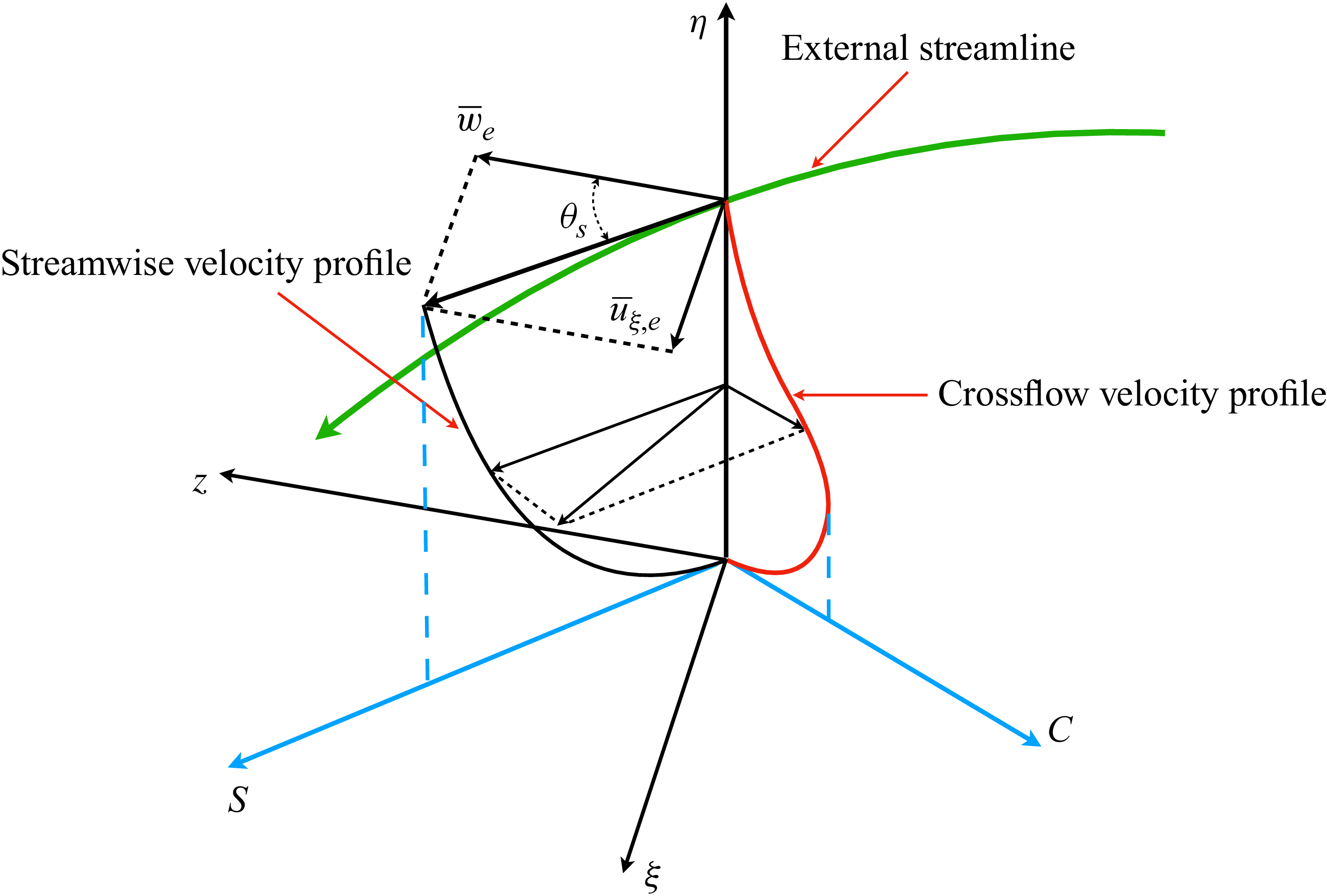
 S
 C

 λ2=−0.035
 w

 Δξm+
 Δηm+
 Δξm,b+
 Δηm,b+
 (Δη/ηK)m
 ηK
 Reτal
 Reτex

 λ2
 λ2=−0.35
 w
 λ2=−0.35
 U∞2/l0∗2

 (a)
 w¯
 uξ¯
 ξ1
 ξ3
 ξ5
 ξ7
 (b)
 θs
 ξ

 u¯s
 u¯c
 ξ1
 ξ3
 ξ5
 ξ7

 (a)
 ξ
 (b)
 ξ
 δK
 ∫0∞(1−(w¯/w∞))dη
 τ¯w,s
 τ¯w

 (a)
 Cf
 Ch
 ξ
 (b)
 ξ

 θs,s
 θs
 θw,s

 ξ
 (a)
 ρ¯us″us″~/τ¯w
 (b)
 ρ¯uc″uc″~/τ¯w
 (c)
 ρ¯uη″uη″~/τ¯w
 (d)
 ρ¯us″uη″~/τ¯w
 (e)
 ρ¯us″uc″~/τ¯w
 (f)
 ρ¯uη″uc″~/τ¯w

 α1
 ξ
 (a)
 h∗
 (b)
 η

 Pk+
 ϕϵk+
 ξ

 Sk/ϕϵk
 h∗
 η
 S=(2SijSij)1/2
 k
 ϕϵk

 ξ1,ξ3,ξ5,ξ7
 kzEww
 kzEuξuξ
 kzETT

 ξ
 (a)
 ρus′′T′′¯/ρuτTw¯
 S
 (b)
 ρuη′′T′′¯/ρuτTw¯
 η
 (c)
 ρuc′′T′′¯/ρuτTw¯
 C

 ξ
 (a)
 −Rus′′T′′
 (b)
 −Ruc′′T′′

 x
 y
 (a)
 (b)
 z



