
1. Introduction
Entering the atmosphere of a planet is one of the most challenging exercises of space exploration missions. The extreme velocities involved in space travel are converted into temperatures rising up to 10 000 K through the compression shock forming in front of a spacecraft. Under such conditions, the gas constituting the atmosphere dissociates into a mixture of ionized species and free electrons, reaching a state called plasma. To protect spacecraft from these harsh conditions, thermal protection systems (TPS) made of either reusable or ablative materials must be carefully designed. For this purpose, TPS material properties and high enthalpy flow models are investigated in specific wind tunnel facilities able to generate and sustain plasma jets during long run times. Two main technologies can be distinguished: arc jets able to reach extreme heat fluxes on large samples such as the Scirroco facility (Marieua et al. Reference Marieua, Reynierb, Marraffab, Vennemannb, De Filippisc and Caristiac2007), and inductively coupled plasma (ICP) facilities providing cleaner flows but limited to lower powers, such as the von Karman Institute (VKI) Plasmatron (Bottin et al. Reference Bottin, Carbonaro, Chazot, Degrez, Abeele, Barbante, Paris, Van Der Haegen, Magin and Playez2004). However, both types of facility are subject to complex unsteady flow behaviours due to both hydrodynamic and magnetic phenomena, eventually degrading the reproduction of flight boundary layer conditions on material samples or probes. A possible approach to understanding these phenomena was explored by Colombo, Ghedini & Sanibondi (Reference Colombo, Ghedini and Sanibondi2010), Shigeta (Reference Shigeta2013) and Trelles (Reference Trelles2013) and relies on time-accurate simulations of whole facilities, considering the coupling of magnetic and fluid domains within large eddy simulations. However, the results obtained are mostly case dependent and remain computationally expensive. On another note, high speed camera observations of plasma jet oscillations in VKI Plasmatron (Cipullo et al. Reference Cipullo, Helber, Panerai, Zeni and Chazot2014) enabled the experimental identification of two distinct sets of perturbations: high frequency pulses linked to the periodic power fluctuations in the electrically conductive region of the jet, and hydrodynamic instabilities at lower frequencies in the test chamber. To the authors’ knowledge, hydrodynamic instabilities of quasi-neutral plasma jets have yet to be investigated, and will be the focus of the present work, as an alternative to costly time-accurate simulations.
As reported early on by Michalke (Reference Michalke1984), jet instabilities have been extensively studied in the literature using the local (one-dimensional) linear stability theory (LST), following the growing interest in jet propulsion and mixing optimization of engine injectors. Among open shear flows, configurations such as heated jets, mixing layers with strong counter flows and wakes with sufficient Reynolds numbers are generally described as flow oscillators (Huerre Reference Huerre2000), exhibiting coherent structures beating at a distinct frequency and relatively insensitive to low noise. This particular behaviour has been correlated with the presence of absolute instabilities in heated round jets in the theoretical work of Monkewitz & Sohn (Reference Monkewitz and Sohn1988), and later experimentally confirmed by Monkewitz et al. (Reference Monkewitz, Bechert, Barsikow and Lehmann1990). The concept of absolute instability had been previously developed by Briggs (Reference Briggs1964) and Bers (Reference Bers1984) for plasma physics, along with the criterion identifying the instability nature bearing their names, and was first applied to continuum flow stability by Huerre & Monkewitz (Reference Huerre and Monkewitz1985).
Since these initial studies, the influence of flow parameters on the transition from convective to absolute instabilities has been broadly investigated using reduced jet models, based on analytical functions and simplified thermo-transport properties (TTP). A well-known result is the threshold value of jet-to-ambient density ratio  $S=0.72$ promoting absolute instabilities in inviscid round jets with thin shear layers found by Monkewitz & Sohn (Reference Monkewitz and Sohn1988). Computations using the spatio-temporal formulation of the LST have accounted for the delaying effect of increasing the Mach number, azimuthal wavenumber or viscosity on the convective to absolute transition: (Monkewitz & Sohn Reference Monkewitz and Sohn1988; Lesshafft & Huerre Reference Lesshafft and Huerre2007; Rees & Juniper Reference Rees and Juniper2010). The effect of confinement on round and planar jets and wakes was investigated by Juniper (Reference Juniper2006, Reference Juniper2008), revealing that confinement effect on absolute instabilities is non-negligible, yet depends on the confinement parameter. More recently, these analyses were extended to co-axial jet flows by Balestra, Gloor & Kleiser (Reference Balestra, Gloor and Kleiser2015), revealing more complex absolute modes than the traditional jet-column and shear-layer modes identified, among others, by Lesshafft & Huerre (Reference Lesshafft and Huerre2007).
Although the previously mentioned studies rely on the local LST, recent advances in computations of larger scale instability mechanisms with direct numerical simulations (DNS) and two-dimensional LST (also called biglobal stability) have shown some of the links between local stability results and the characteristics of global modes sustained by absolutely unstable flows (Chomaz Reference Chomaz2005). A comparison of LST, DNS and experimental results allowed Coenen & Sevilla (Reference Coenen and Sevilla2012) to find the relation between the length and position of the region of local absolute instability and the formation of global stability features. Along with Lesshafft, Huerre & Sagaut (Reference Lesshafft, Huerre and Sagaut2007) and Nichols, Schmid & Riley (Reference Nichols, Schmid and Riley2007), they further showed that global modes tend to pulse near the absolute frequency found with LST at the most upstream position of the absolute region.
However, even if local linear stability analyses are relevant to predict heated jet oscillations, the simplified base state and TTP models used in most of the previous studies suffer the comparison to more realistic cases. Bearing this in mind, recent LST studies of absolute instabilities have focused on more physically sound base states (Coenen, Sevilla & Sanchez Reference Coenen, Sevilla and Sanchez2008; Coenen & Sevilla Reference Coenen and Sevilla2012), yielding surprising results with respect to reduced models. Lesshafft & Marquet (Reference Lesshafft and Marquet2010) observed that, even with a uniform density field, instabilities can develop an absolute nature in cases where the maximum shear is located in low velocity regions of the jet. This behaviour seems to be linked with the apparent decrease of the group velocity at the velocity perturbations maximum. Similar results have also been observed by Balestra et al. (Reference Balestra, Gloor and Kleiser2015) in co-axial jets. Furthermore, Nichols et al. (Reference Nichols, Schmid and Riley2007) observed that absolute instabilities intensified when the maximum shear aligns with the density shear in heated round jets. This feature was previously hinted at by the leading role of the baroclinic torque on absolute instabilities found by Lesshafft & Huerre (Reference Lesshafft and Huerre2007).
Results obtained using reduced models may further suffer from the prescription of simplified thermo-transport properties and the independence of dimensionless numbers from each other, which can lead to unrealistic base states. These concerns were already expressed by Coenen & Sevilla (Reference Coenen and Sevilla2012) based on observations of Sanchez-Sanz, Sanchez & Linan (Reference Sanchez-Sanz, Sanchez and Linan2006) and Sanchez-Sanz, Rosales & Sanchez (Reference Sanchez-Sanz, Rosales and Sanchez2010). Such effects are expected to be particularly present for plasma jets, where the calorically perfect gas assumption breaks down due to high temperature effects. As showcased by Malik & Anderson (Reference Malik and Anderson1991) for hypersonic boundary layers, stability results are influenced by the departure of the TTP from low temperature models, such as Sutherland's law for viscosity, once the first dissociation reaction effects appear. Recent work on hypersonic boundary layers by Miró Miró et al. (Reference Miró Miró, Beyak, Pinna and Reed2019) has further shown the influence of using different high temperature TTP models on LST results. The integration of equilibrium chemistry in parabolized stability equations by Zanus, Miró Miró & Pinna (Reference Zanus, Miró Miró and Pinna2019) revealed different effects depending on the instability mode considered. To the authors’ knowledge, there is, however, no account of high temperature effects on the switch from convective to absolute instabilities in the literature.
The present project aims at covering these gaps in hydrodynamic instabilities by studying a plasma jet stability by means of the local spatio-temporal LST. This work uses realistic flow profiles obtained from magneto-hydrodynamic simulations of the VKI Plasmatron facility, Bottin et al. (Reference Bottin, Carbonaro, Chazot, Degrez, Abeele, Barbante, Paris, Van Der Haegen, Magin and Playez2004). Special attention is given to the analysis of absolute regions. The evolution of instabilities that could be triggered by a noisy environment is analysed by carrying out the full impulse response of the wavepacket to an impulse. The influence of high temperatures on the jet stability is studied with state-of-the-art high enthalpy flow models.
2. Problem and model description
2.1. Geometry
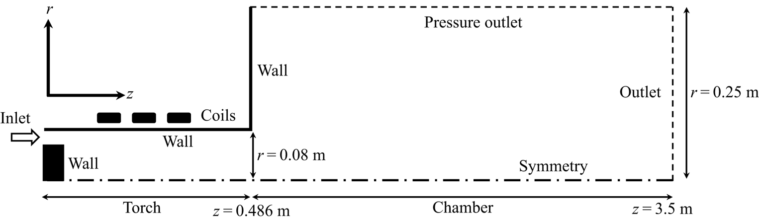
The geometry investigated is shown in figure 1, and represents a simplified axisymmetric version of the torch and test chamber sections of the plasma wind tunnel. The plasma is generated by induction heating of a test gas injected into the torch through an annular inlet, and is blown in the test chamber forming a coaxial round jet. In practice, the swirling of the jet is prevented by the presence of a foam piece before the inlet, and simulations will consider a null azimuthal velocity. For the rest of this study, the coordinates  $(r,\theta ,z)$ are used to describe namely the radial, azimuthal and streamwise directions. This work investigates different test cases obtained by varying the main driving parameters of the facility, respectively the static pressure in the test chamber noted
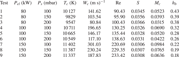
 $P_s$ and the power transmitted through induction by the coils to the flow noted
 $P_{el}$. A summary of the conditions studied is given in table 1. Pressures are kept above 100 mbar to maintain the flow in equilibrium, based on experimental observations of Cipullo et al. (Reference Cipullo, Helber, Panerai, Zeni and Chazot2014). Although the jet is horizontal, no buoyancy effects are observed in the facility for powers under 200 kW and below 250 mbar, and are therefore also ignored here. A third driving parameter is usually considered in experiments, namely the mass flow
 $\dot {m}$ injected at the torch inlet. In the present study
 $\dot {m}$ is kept constant at 16 g s
 $^{-1}$ and its influence is not considered. The reference length used throughout this work is the torch radius
 $l_{ref}=r_{torch}=0.08\ \textrm {m}$.
Sketch of the computational domain used for Plasmatron simulations. The main dimensions and boundary conditions are indicated.

Parameters defining each test case studied, along with main quantities and non-dimensional numbers at the chamber inlet.

2.1.1. Simulations of the plasma wind tunnel
Simulations are carried out within the open source Computational Object-Oriented Library for Fluid Dynamics CoolFluid-ICP (Lani Reference Lani2008), relying on a second-order spatially accurate finite-volume solver, and an implicit Newton procedure to reach a steady state solution. Both the magnetic and fluid fields are considered by weakly coupling the Maxwell equations to the compressible Navier–Stokes equations. The resulting flow equations are summarized in their dimensional form below
 \begin{gather} \frac{\partial}{\partial t}(\rho)+\boldsymbol{\nabla}\boldsymbol{\cdot}(\rho \boldsymbol{u})=0, \end{gather}
 \begin{gather}\frac{\partial}{\partial t}(\rho\boldsymbol{u})+\boldsymbol{\nabla}\boldsymbol{\cdot}(\rho\boldsymbol{u}\otimes\boldsymbol{u}) = -\boldsymbol{\nabla} p + \boldsymbol{\nabla}\boldsymbol{\cdot}\tau + \mathcal{F}_L, \end{gather}
 \begin{gather}\frac{\partial}{\partial t}(\rho E)+\boldsymbol{\nabla}\boldsymbol{\cdot}(\rho H\boldsymbol{u}) = \boldsymbol{\nabla}\boldsymbol{\cdot}\tau\boldsymbol{\cdot}\boldsymbol{u} - \boldsymbol{\nabla}\boldsymbol{\cdot}\boldsymbol{q}+\mathcal{P}_J, \end{gather}
where  $\tau$ is the viscous stress tensor,
 $E$ the total energy defined as
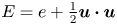 $E=e+\frac {1}{2}\boldsymbol {u}\boldsymbol {\cdot }\boldsymbol {u}$ with the specific energy
 $e$,
 $H$ is the total enthalpy given by
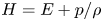 $H=E+{p}/{\rho }$ and
 $\boldsymbol {q}$ is the heat flux vector. The coupling is done through Joule heating
 $\mathcal {P}_J$ and the Lorentz force
 $\mathcal {F}_L$ respectively in the energy and momentum equations, and the temperature dependence of the gas electric conductivity. The reader is referred to Zhang, Lani & Panesi (Reference Zhang, Lani and Panesi2016) for a complete breakdown of the variables and electromagnetic equations. Details of the implementation are available in the reports of Honzatko (Reference Honzatko2006) and Prokop (Reference Prokop2007). Thermodynamic and transport properties of the gas are obtained using the Mutation
 $^{++}$ library developed by Scoggins & Magin (Reference Scoggins and Magin2014), assuming an 11-species air mixture including (N, O, NO, N2, O2, N
 $+$, O
 $+$, NO
 $+$, N2
 $+$, O2
 $+$, e
 $-$) in LTE. It is worth noting that such mixture allows for ionization effects on the flow properties.
An open boundary condition allowing for entrainment of gas is imposed at the top edge of the computational domain: homogeneous Neumann conditions are imposed on all quantities except for the pressure which is set to the desired  $P_s$. A subsonic outflow condition is set at the outlet, no-slip isothermal walls are considered with
 $T_{wall}=350\ \textrm {K}$ to mimic the cooled walls of the facility. At the inlet, the streamwise velocity is imposed through the mass flow
 $\dot {m}$, the pressure is interpolated from the interior of the domain and the temperature is set to the wall value. The convergence of the solution is investigated by computing results on a series of meshes with increasing definition. For our set-up, a mesh of
 $23.10^3$ elements is enough to approach results of the finest mesh with precision of 0.03 % of the maximum temperature and 0.06 % of the maximum velocity. However, the solution does not provide second derivatives of flow quantities, and an algebraic model is fit to the simulations.
2.1.2. Base state
Our algebraic model is built by interpolating the non-dimensional streamwise velocity and temperature radial profiles at  $177$ discrete streamwise positions along the test chamber. The interpolation is carried out in Matlab® using the fit routine. The following expressions were found to reproduce the flow field for the range of conditions studied and streamwise positions from
 $z=0.5$ to
 $z=3.5\ \textrm {m}$:
 \begin{align} W(r) &= a_WGN(r, 0, b_W) + c_W(1-\tanh[d_W(r - e_W)]) \nonumber\\ &\quad + f_W(1-\tanh[g_W(r - h_W)])GN(r,i_W,j_W)r^2, \end{align}
 \begin{align} T(r) &= a_TGN(r, 0, b_T)+ c_T(1- \tanh[d_T(r - e_T)]) + f_T(1 - \tanh[g_T(r- h_T)]) \nonumber\\ &\quad + i_T(1 - \tanh[j_T(r - k_T)]), \end{align}
 \begin{equation} GN(r,\mu,\sigma) = \frac{1}{\sigma\sqrt{2{\rm \pi}}}\exp({{-\left(r-\mu\right)^2}/{2\sigma^2}}),\end{equation}
where  $W$ and
 $T$ denote the streamwise velocity and temperature along the non-dimensional radial coordinate
 $r$. Values of the coefficients (
 $a_W, b_W,\ldots$) resulting from the interpolation are then used to obtain the analytical derivatives of the profile quantities. The error introduced by the interpolation remains bounded by respectively
 $0.4\,\%$ and
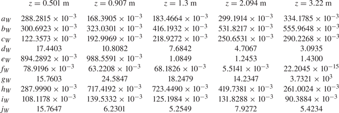
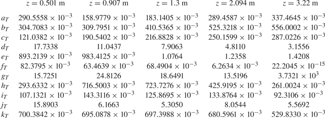
 $0.15\,\%$ of the temperature and velocity at the chamber inlet centreline with respect to simulation results. Examples of the interpolation coefficients for different streamwise positions are given in tables 4 and 5 in appendix A.
Thermodynamic and transport properties involved in the stability equations are reconstructed from the temperature profiles and constant pressure  $P_s$ by assuming the same mixture in LTE as in the simulations. Flow properties are computed in the Vesta toolkit as it also evaluates derivatives of the properties with respect to pressure and temperature. We have observed that derivatives of the Mutation
 $^{++}$ properties numerically reconstructed exhibit a noisy behaviour, which is found to greatly impact the stability results. The equilibrium composition is obtained from the Dekaf boundary layer solver (Groot et al. Reference Groot, Miró Miró, Beyak, Moyes, Pinna and Reed2018), which solves the equilibrium system based on partial pressure (Miró Miró et al. Reference Miró Miró, Beyak, Mullen, Pinna and Reed2018) while enforcing the ambipolar condition. Transport properties are obtained similarly to Scoggins & Magin (Reference Scoggins and Magin2014): using approximations to Chapman and Enskog's expansion using Laguerre–Sonine polynomials following Magin & Degrez (Reference Magin and Degrez2004). Collisional data required for such properties are obtained from the latest references included in Mutation
 $^{++}$, ignoring both frozen and reactive barodiffusion, together with elemental demixing. Thermal properties are retrieved from the NASA polynomial database (McBride, Gordon & Reno Reference McBride, Gordon and Reno1993), and the mixing rules are applied to obtain the mixture quantities. More details about these models are available in Miró Miró et al. (Reference Miró Miró, Beyak, Pinna and Reed2019).
In order to assess the influence of the LTE assumption on the stability for a given base state, a second set of properties is reconstructed from the simulations by assuming a calorically perfect gas (CPG). The viscosity is retrieved using Sutherland's law, and a constant Prandtl number is imposed  $Pr=\mu c_p/\kappa =0.7$, where
 $c_p$ is the air isobaric specific heat capacity,
 $\mu$ is the viscosity and
 $\kappa$ is the thermal conductivity.
Quantities involved in the stability equations are made non-dimensional with respect to the local centreline quantities denoted by the subscript ‘ $_c$’, except for the reference pressure chosen as
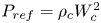 $P_{ref}=\rho _cW_c^2$. The main non-dimensional numbers involved in the LTE stability equations are given by
 \begin{equation} Re = \frac{\rho_c~W_c~l_{ref}}{\mu_c},\quad Pr=\frac{\mu_ch_c}{\kappa_c\,T_c},\quad Ec = \frac{W_c^2}{h_c}, \end{equation}
where  $Re$,
 $Pr$ and
 $Ec$ are the Reynolds, Prandtl and Eckert reference numbers, the static enthalpy is noted
 $h$ and the density
 $\rho$.
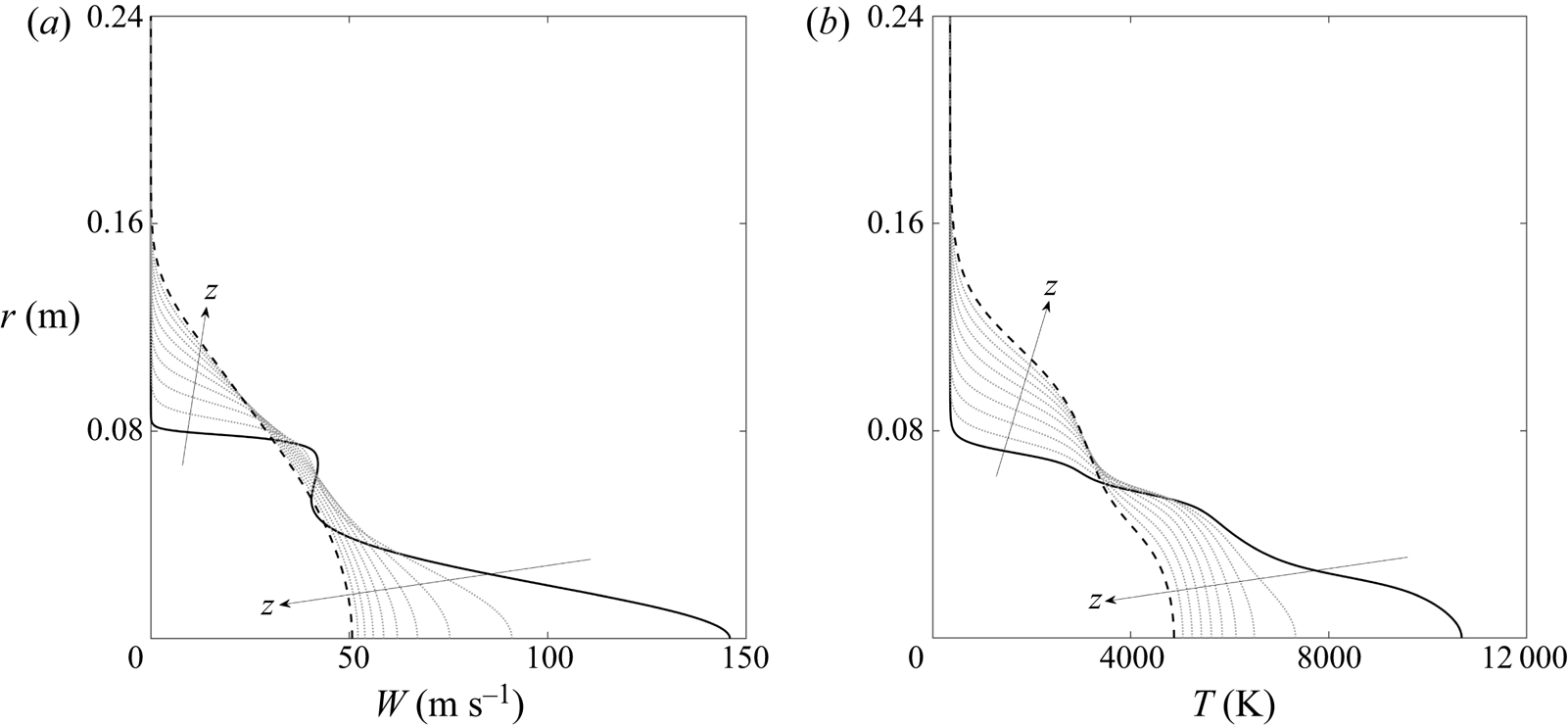
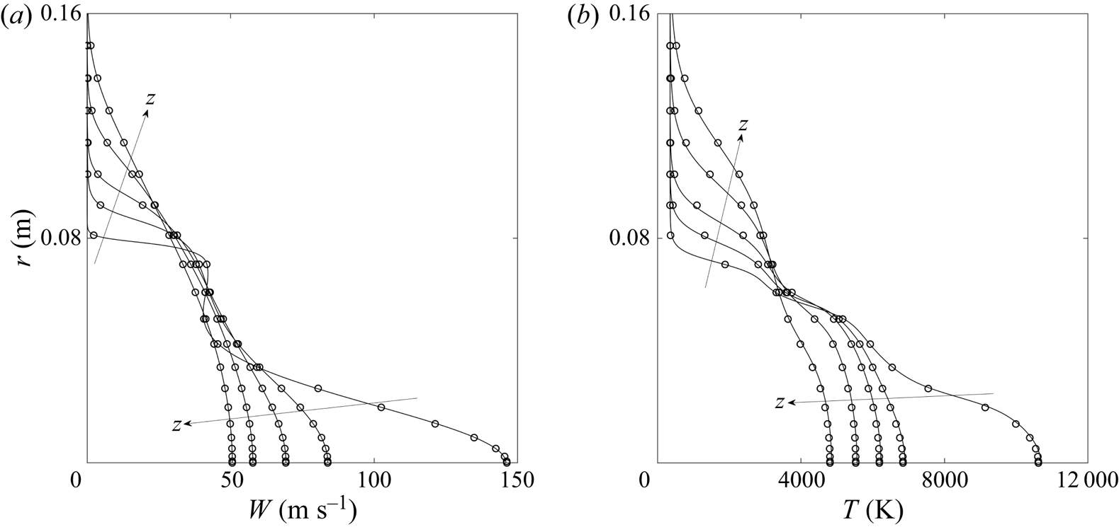
Examples of dimensional velocity and temperature profiles obtained after the analytical interpolation are given in figure 2 for  $P_{el}=100\ \textrm {kW}$ and
 $P_s=150\ \textrm {mbar}$, while corresponding profiles of the equilibrium flow properties are displayed in appendix A.2. Velocity profiles at the chamber inlet exhibit two streams and shear layers, similarly to coaxial jets studied in the literature (Balestra et al. Reference Balestra, Gloor and Kleiser2015). The main stream is caused by the heating at the jet centreline, while the secondary stream originates from the annular inlet. The bypass ratios defined as:
 $h_{\text {b}}=W_c/W_s$, where
 $W_s$ is the averaged velocity of the secondary stream, ranges from low to mid values (
 $h_{\text {b}}\in [0.18;\ 0.43]$) depending on the driving parameters. For all cases, the primary shear is much thicker than the secondary one. Humps observed in the temperature profiles are due to the evolution of the equilibrium gas composition with temperature, and are not linked to the velocity profiles as the viscous heating is negligible. Further downstream, the jet displays a single stream, with a large shear-layer thickness similar to the configurations studied by Lesshafft & Huerre (Reference Lesshafft and Huerre2007).
Analytical profiles of Plasmatron velocity (a) and temperature (b) for  $P_{el}=100\ \textrm {kW}$ and
 $P_s=150\ \textrm {mbar}$ along the test chamber, from
 $z=0.5\ \textrm {m}$ (
 $-$) to
 $z=3.5\ \textrm {m}$ (- -), with intermediate profiles (
 $\cdots$) linearly spaced between the inlet and outlet.

Although not displayed here, an increase of the electric power  $P_{el}$ increases both the centreline temperature and velocity at the chamber inlet, while an increase in pressure
 $P_s$ is found to decrease the centreline velocity and to have little impact on the temperature field. In addition, increasing the power decreases the bypass ratio at the inlet which results in more slender velocity profile; in contrast, changes in the pressure are found to act as a scaling of the overall velocity profiles while having less influence of the bypass ratio.
The different test cases are summarized in the table 1, along with the main dimensional quantities and non-dimensional numbers taken at the inlet of the test chamber. The temperature ratio between the surrounding gas and the jet centreline is introduced as  $S=T_{\infty }/T_c$, where
 $T_{\infty }=T_{wall}=350\ \textrm {K}$. One can note that the Mach number presented in table 1 is computed using the equilibrium speed of sound returned by the Mutation
 $^{++}$ library, taking into account high temperature effects.
2.2. Stability model
This study assumes that Plasmatron's jet is slowly evolving along the streamwise direction and can be locally approximated as a parallel flow. This is supported by the fact that derivatives of the base state quantities with respect to the radial dimension are in average two orders of magnitude larger than with respect to the streamwise direction. The local formulation of the LST is considered, where ( $z, \theta$) are the spectral directions, while
 $r$ is the differential direction. The classical decomposition of the instantaneous flow field is performed:
 $Q(\textbf {x}, t) = \bar {Q}(\textbf {x}) + q'(\textbf {x}, t)$ where
 $\bar {Q}$ is the
 $\textit{O}^1$ base state and
 $q'$ is the related
 $\textit{O}^\epsilon$ perturbation quantity. The natural path to transition as defined by Morkovin, Reshotko & Herbert (Reference Morkovin, Reshotko and Herbert1994) is considered, and the perturbations are modally decomposed
 \begin{equation} q'(r,\theta,z,t) =\tilde{q}(r)\exp({\textrm{i}(\alpha z + m\theta -\omega t )}) +\textrm{c.c.}, \end{equation}
where  $\tilde {q}$ is the complex amplitude function,
 $\alpha$ and
 $m$ are respectively the streamwise and integral azimuthal wavenumbers. The complex angular frequency is
 $\omega$ and c.c. denotes the complex conjugate necessary to retrieve real perturbations. Introducing (2.4) and the quantities’ decomposition into the flow equations, one obtains the stability equations, which reduce to a generalized eigenvalue problem once completed with the appropriate set of boundary conditions.
Stability equations are derived within the Automatic Derivation and Implementation module (Adit) of the Vesta toolkit (Pinna & Groot Reference Pinna and Groot2014) from the compressible Navier–Stokes equations in cylindrical coordinates. The influence of the magnetic field is ignored as it is mainly confined to the torch section of Plasmatron. The state vector considered is [ $u', v', w', T', p'$], namely the components of the velocity along
 $(r,\theta ,z)$, the temperature and pressure. The stability equations include high temperature effects by expanding the transport properties, similar to the dynamic viscosity
 \begin{equation} \mu = \bar{\mu} + \frac{\textrm{d}\bar{\mu}}{\textrm{d}\bar{T}}T' + \frac{\textrm{d}\bar{\mu}}{\textrm{d}\bar{P}}p', \end{equation}
where the derivatives of the transport properties with respect to pressure and temperature are obtained as described in § 2.1.2. Stability equations for a jet in LTE are described in appendix B.1. The main differences between the current implementation of the LTE system with respect to more common low temperature compressible stability equations come from the introduction of the  $F$ and
 $G$ variables introduced by Malik & Anderson (Reference Malik and Anderson1991) to modify the equation of state given in (2.6a).
 \begin{gather} \tilde{\rho}=\frac{\bar{F}\bar{\rho}}{\bar{P}}\tilde{p} - \frac{\bar{G}\bar{\rho}}{\bar{T}}\tilde{T}, \end{gather}
 \begin{gather}\bar{F} = 1 - \left.\frac{\partial \ln \zeta}{\partial \ln P}\right|_T, \quad \bar{G} = 1 - \left.\frac{\partial \ln \zeta}{\partial \ln T}\right|_P, \end{gather}
where  $\zeta$ is the compressibility factor of the gas mixture in LTE. Unless specified otherwise, the stability equations solved in this work assume a flow in LTE. Stability analyses using the CPG assumption eliminate the dependence of the transport properties on the pressure and rely on the classical state equation.
Homogeneous Dirichlet conditions are imposed at the far field ( $r\rightarrow \infty$) to yield vanishing perturbations. At the centreline, a set of boundary conditions is derived to cope with the apparent singular nature of the coordinates in a similar manner to Lesshafft & Huerre (Reference Lesshafft and Huerre2007). Equations for the perturbation centreline conditions depend on the value of
 $m$ and are given in appendix B.3.
Similarly to Huerre (Reference Huerre2000), the spatio-temporal formulation of the LST is used to study the absolute/convective nature of instabilities, thus,  $\alpha$ and
 $\omega$ are both complex numbers. Absolute instabilities are detected when a localized impulse promotes self-sustained perturbations through a resonance mechanism in the flow. This is interpreted as an infinite growth of instabilities with null group velocity
 $v_{{g}}=x/t$ in the long-time limit after the impulse. In practice, Briggs and Bers provided a simple criterion to identify the nature of instabilities from isocontours of the spatio-temporal growth rate
 $\sigma =\textrm {Im}(\omega )$ in the complex wavenumber plane
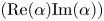 $(\textrm {Re}(\alpha ) \textrm {Im}(\alpha ))$. The sign of
 $\sigma$ where the contours describe a saddle point (noted ‘
 $\sigma _S$’) is related to the long-time limit of the perturbations at
 $v_{{g}}=0$. When
 $\sigma _S>0$, the flow is absolutely unstable, while for
 $\sigma _S\leq 0$ the flow is either stable or convectively unstable. However, to respect the criterion, valid saddles must be pinched between an
 $\alpha ^+$ and an
 $\alpha ^-$ branch. Starting at the saddle point, contours of growing
 $\sigma =\omega _i$ must reach respectively the
 $\textrm {Im}(\alpha ) > 0$ and
 $\textrm {Im}(\alpha ) < 0$ half-planes. Therefore the flow is absolutely unstable only if
 $\omega _i>0$ at a valid saddle point.
2.3. Numerical implementation
The stability equations reduced to a generalized eigenvalue problem are solved imposing the complex wavenumber  $\alpha$ and integer
 $m$ in the Vesta toolkit (Pinna Reference Pinna2013), relying on the ZGEEV Lapack routine. Stability equations are discretized using the pseudo-spectral Chebyshev collocation method (Trefethen Reference Trefethen2000). The discretization in the radial direction is further modified by using a tangential mapping technique (Bayliss & Turkel Reference Bayliss and Turkel1992) described in appendix B.2 and implemented by Esposito (Reference Esposito2016). A number of collocation points set to
 $N=201$ is sufficient to reach a convergence of order
 $10^{-7}$ on the eigenvalues obtained for the conditions studied in this work. In practice, the construction of the eigenvalue problem matrices is
 $40\,\%$ slower in LTE than for the CPG problem. However, the two solvers take roughly the same time to compute the eigenvalue spectrum.
A local eigenvalue solver based on Newton's iterative method is used to obtain individual eigenvalues from a first guess (Pinna Reference Pinna2013). This solver is used to track eigenvalues across the complex wavenumber plane. Saddle points are found by approaching  ${\partial \omega }/{\partial \alpha } = 0$ using the trust-region dogleg algorithm (Powell Reference Powell1968) integrated in the Matlab®fsolve routine. Saddle points are tracked for variations of the streamwise position and group velocity using the same methods.
3. Absolute instability analysis
3.1. Analysis at the inlet
Stability features of the plasma jet are analysed in detail assuming  $P_{el}=100\ \textrm {kW}$ and
 $P_s=150\ \textrm {mbar}$, corresponding to the case number
 $5$ of table 1. The global spectra of eigenvalues obtained for
 $N=201$ and
 $N=301$, imposing
 $\alpha =1$ and
 $m=0$ at the inlet of the chamber (
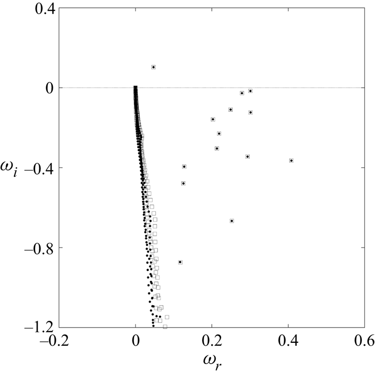
 $z=0.5\ \textrm {m}$) are displayed in figure 3. The present spectrum is composed of continuous branches, a set of stable discrete modes and a single unstable mode. The set of discrete stable modes is converged, and remains under the
 $\omega _r$ axis for real values of
 $\alpha$. The unstable mode is found at
 $\omega = 0.0473 + 0.1027i$ for the current wavenumber value, and it is the mode tracked with the local solver to draw the contour plots used in the spatio-temporal analysis.
Spectrum of eigenvalues obtained by imposing  $\alpha =1$ and
 $m=0$ for the test case 5 at
 $z=0.5$ m with
 $N=201$ (
 ) and
 $N=301$ (
 ) discretization points.

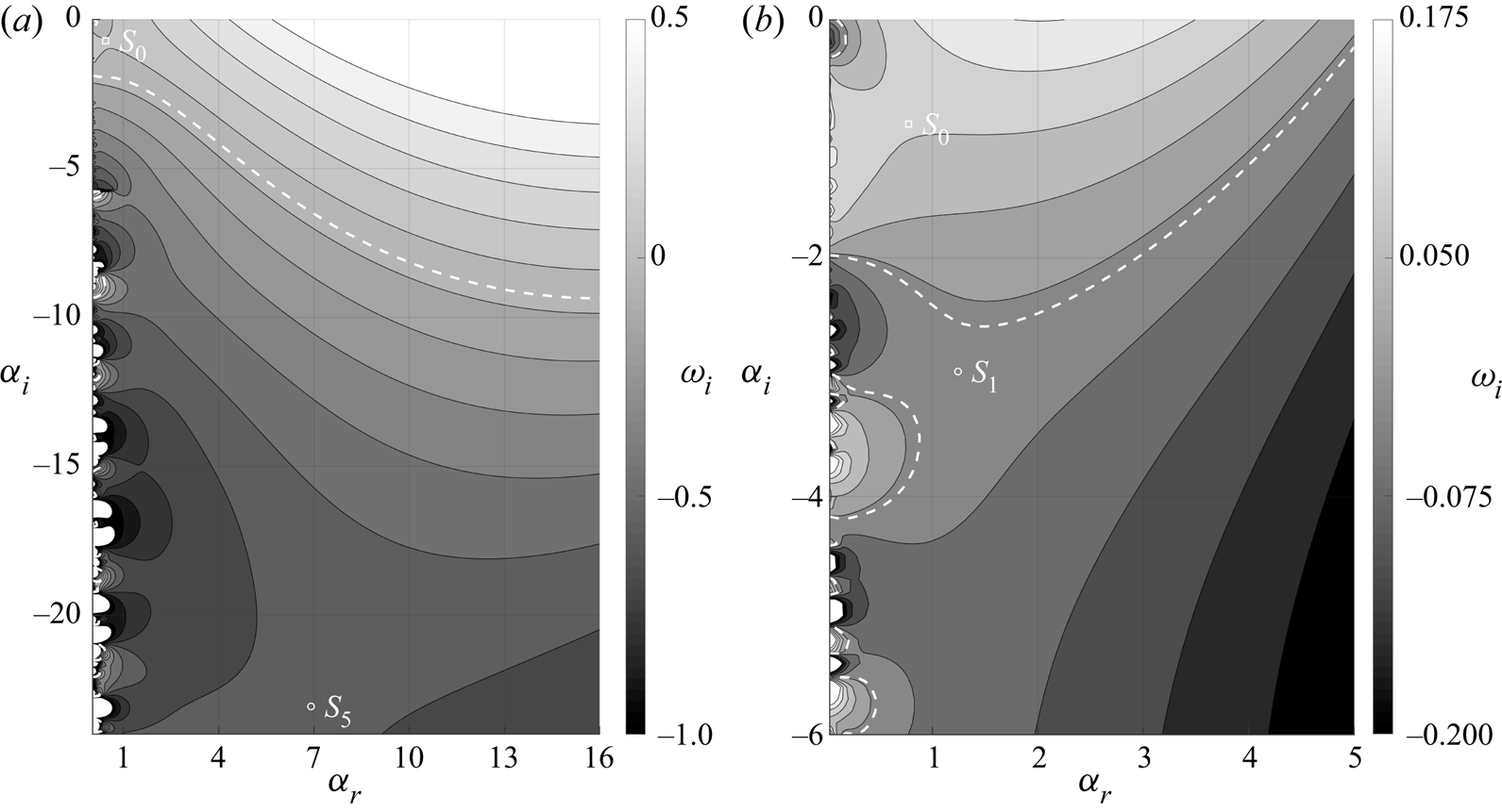
Contours of the spatio-temporal growth rate in the complex wavenumber plane at the chamber inlet are displayed in figure 5(a) for axisymmetric perturbations. At the inlet, the base state is akin to the family of coaxial jets studied by Balestra et al. (Reference Balestra, Gloor and Kleiser2015), although the core shear-layer thickness is significantly larger than that of the secondary shear. The saddle point with largest spatio-temporal growth rate at this station is found near the origin of the axis. This saddle is noted  $S_0$ for the rest of this study, its absolute wavenumber is
 $\alpha _{S0}=0.4856 - 0.7902i$ and absolute non-dimensional frequency is
 $\omega _{S0}=0.0881 + 0.0739i$. As the saddle is pinched between an
 $\alpha ^+$ and an
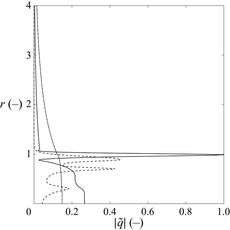
 $\alpha ^-$ branch, while displaying a positive growth rate, the flow is absolutely unstable for this case and at this position. The absolute value of the perturbation functions related to
 $S_0$ are shown in figure 4. The pressure
 $\tilde {p}$ and streamwise velocity
 $\tilde {w}$ perturbations are amplified both at the centreline and in the secondary stream shear layer (
 $r=1$). Such shapes are similar to both the mixed modes described by Lesshafft & Huerre (Reference Lesshafft and Huerre2007) in top-hat jets with thick shear layers and outer modes described by Balestra et al. (Reference Balestra, Gloor and Kleiser2015) in coaxial jets. This is further explained by the fact that
 $S_0$ is pinched between an
 $\alpha ^-$ branch of jet-column modes located near the
 $\alpha _i$ axis, and an
 $\alpha ^+$ branch of shear-layer modes coming from the upper
 $\alpha _i>0$ half plane. The mixed mode at saddle
 $S_0$ exhibits a low dimensional frequency of
 $f_{S0}=\textrm {Re}(\omega _{S0})W_c/(2{\rm \pi} l_{ref})=25.62\ \textrm {Hz}$ and a large wavelength
 $\lambda _{S0}=2{\rm \pi} l_{ref}/ \textrm {Re}(\alpha _{S0})=1.035\ \textrm {m}$.
Magnitude of  $S_0$ perturbation functions with
 $m=0$ in case 5 at
 $z=0.5$ m. The perturbation variables are
 $\tilde {w}$ (
 $-$),
 $\tilde {T}$ (- -),
 $\tilde {p}$ (
 ), and are normalized by
 $\max (|\tilde {w}|)$.

Following Huerre & Monkewitz (Reference Huerre and Monkewitz1990, p. 487), the absolute wavelength is compared to the development length of the flow  $L = \theta (\partial \theta /\partial z)^{-1}$, where
 $\theta$ is the momentum thickness of the profile. It appears that the ratio
 $\epsilon =\lambda _{S0}/L$ is close to unity at the inlet of the jet, preventing a possible connection between local and global stability properties. However, results from the local stability analysis are still believed to be insightful on the presence of global modes, as the absolute regions discussed in the following sections extend to jet regions where
 $\epsilon \ll 1$.
A series of valid and non-valid saddle points is also observed in figure 5(a) near the  $\alpha _i$ axis, however, displaying smaller growth rates than
 $S_0$ and thus are not considered any further. An additional saddle is present for low values of
 $\alpha _i$ and further away from the vertical axis, noted
 $S_5$, at
 $\alpha _{S5}=6.6581 -23.1098i$ and with
 $\omega _{S5}=1.3731 - 0.5581i$. This mode displays perturbation functions typical from the shear layer modes described by Lesshafft & Huerre (Reference Lesshafft and Huerre2007), at a higher frequency
 $f_{S2}=399.3\ \textrm {Hz}$ and shorter wavelength
 $\lambda _{S5}=0.075\ \textrm {m}$ than
 $S_0$, corresponding roughly to the radius of the secondary shear. Although
 $S_5$ is not linked to an absolute instability, it is highlighted here as it will play a role in the full impulse response described in § 5.
Contours of constant spatio-temporal growth rate  $\omega _i$ for the axisymmetric mode
 $m=0$ at
 $z=0.5$ m (a) and
 $z=2.086$ m (b). The contours are limited to
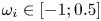 $\omega _i\in [-1; 0.5]$ (a) and
 $\omega _i\in [-0.2; 0.175]$ (b) and the
 $\omega _i=0$ isocontour is highlighted (white dashed line). The least stable saddle is noted
 $S_0$, while
 $S_5$ and
 $S_1$ are the secondary saddles involved in the full impulse response.

Increasing the integral azimuthal wavenumbers to  $m=[1,2]$ is found to decrease the growth rate of
 $S_0$ down to
 $\textrm {Im}(\omega _{S0}) = -0.1663$ at
 $m=2$, while
 $S_0$ moves to lower
 $\alpha _i$ values. Furthermore, for
 $m>0$, the shape of perturbations at
 $S_0$ changes to resemble shear layer modes. In contrast, the shear-layer mode associated with saddle
 $S_2$ is barely affected by the changes in
 $m$, in agreement with results of Lesshafft & Huerre (Reference Lesshafft and Huerre2007) for single top-hat jets. However, similar results for coaxial jets were not included in the work of Balestra et al. (Reference Balestra, Gloor and Kleiser2015) which was restricted to axisymmetric perturbations. One can note that no valid saddle was found to lie on the upper
 $\alpha _i>0$ half-plane in the results presented.
3.2. Influence of the streamwise position
As the jet diffuses in the test chamber, the primary and secondary streams merge to form a single jet with a thick shear layer around  $z=1.5\ \textrm {m}$, which is found to impact the stability behaviour. Contours of the spatio-temporal growth rate are displayed after this station, at
 $z=2.086\ \textrm {m}$, in figure 5(b). No equivalent of the saddle
 $S_5$ is found at this station, however, a saddle similar to
 $S_0$ is still present at
 $\alpha _{S0}=0.6122 - 0.7533i$. The complex frequency at
 $S_0$ is
 $\omega _{S0}=0.2056 + 0.0982i$, which indicates that the flow is still absolutely unstable at this position. Saddles along the
 $\alpha _i$ axis still display lower spatio-temporal growth rates when compared to
 $S_0$. The valid saddle directly beneath
 $S_0$ noted
 $S_1$ in figure 5(b) at
 $\alpha _{S1}=1.0793 - 2.9858i$ and with
 $\omega _{S1}=0.2331 - 0.0090i$ is nonetheless singled out as it will play a role in the full impulse response at this streamwise position. Similarly to the inlet, no valid saddle is found in the upper
 $\alpha$-plane.
In order to better understand the structure of the absolutely unstable region, the saddle  $S_0$ is tracked along the streamwise direction from
 $z=0.5\ \textrm {m}$ to
 $z=3.5\ \textrm {m}$. Streamwise positions beyond
 $z=3.5\ \textrm {m}$ are not considered, as they are not representative of the actual facility. The tracking is done for
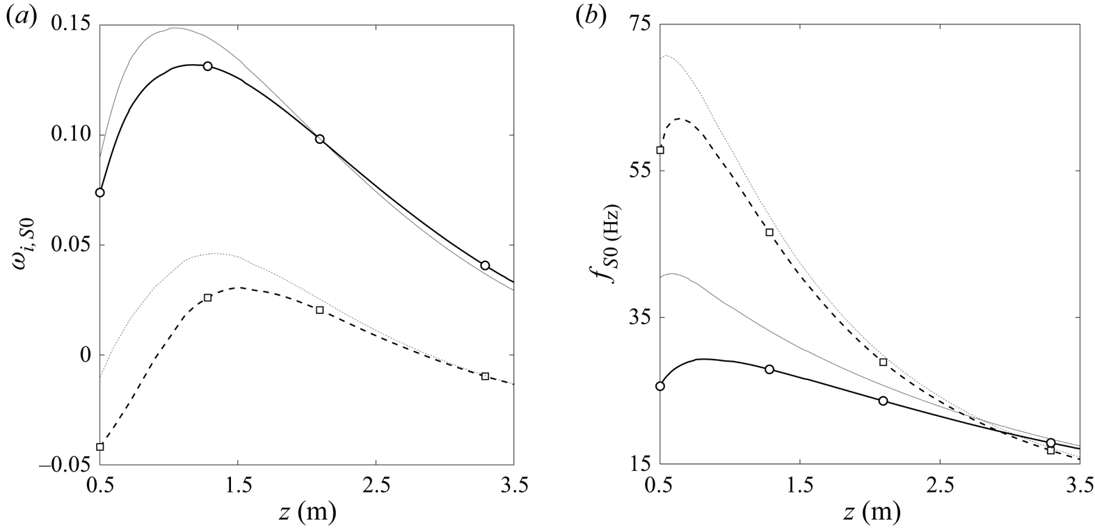
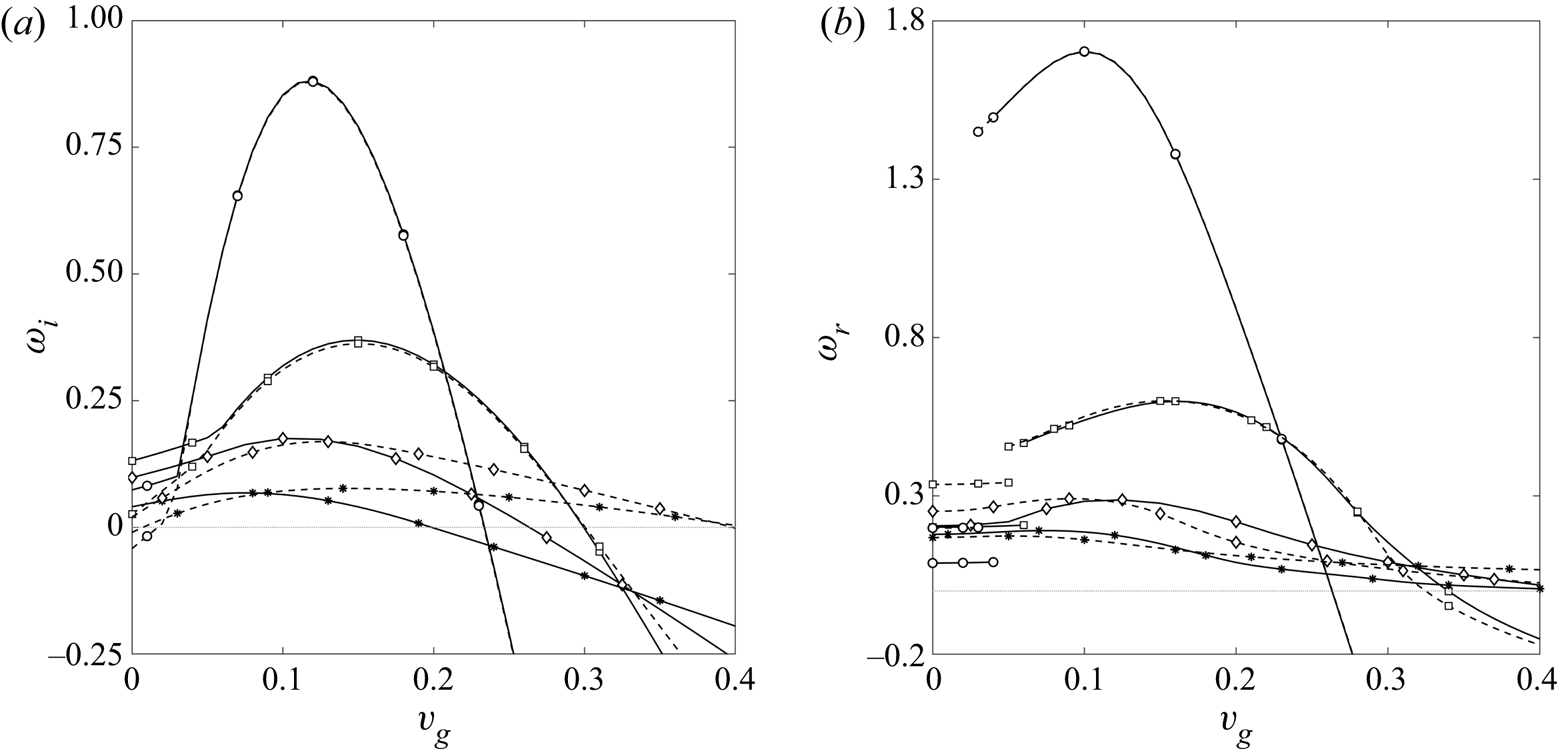
 $m=[0,1]$, with both the CPG and LTE stability solvers. The resulting curves of absolute growth rate and dimensional frequency along the test chamber are displayed in figure 6. The symbols on the curves in figure 6 indicate saddles found by computing the full contours of the growth rate in order to confirm the accuracy of the tracking tool and to make sure no saddle playing a role in the stability behaviour is overlooked. Discontinuities observed in the curves are due to the local nature of the analytical interpolation used to reconstruct the base flow. This tracking confirms that
 $S_0$ in figures 5(a) and 5(b) are the same saddle.
Streamwise evolution of the absolute growth rate (a) and dimensional frequency (b) associated with  $S_0$, for axisymmetric
 $m=0$ (
 $-$) and first helical
 $m=1$ (- -) modes, with the LTE (thick line) and CPG (thin line) stability solvers. The absolute growth rate and frequency of
 $m=0$ (
 ) and
 $m=1$ (
 ) saddle points obtained from full contours are added to confirm the accuracy of the tracking tool.

Results for the axisymmetric modes are analysed first, after which the helical modes are discussed. Axisymmetric modes ( $m=0$) display a positive growth rate along the whole domain considered, which yields a larger region of absolute instability than what is observed in the literature. The positive slope of the growth rate
 $(\partial \sigma /\partial z)$ at the inlet is in agreement with observations of Coenen & Sevilla (Reference Coenen and Sevilla2012) for jets displaying a small shear-layer thickness with respect to the nozzle diameter. This is the case for the inlet profiles studied here only when considering the secondary shear layer (around
 $r=1$ in figure 2), which coincides with the radial position where the amplification of disturbances associated with
 $S_0$ is maximum. The absolute growth rate reaches its maximum value
 $\max (\sigma _{S0})=0.1319$ in the chamber at
 $z_{max}=1.1657\ \textrm {m}$, and the frequency at the start of the absolute region is
 $f_{S0}=25.62\ \textrm {Hz}$.
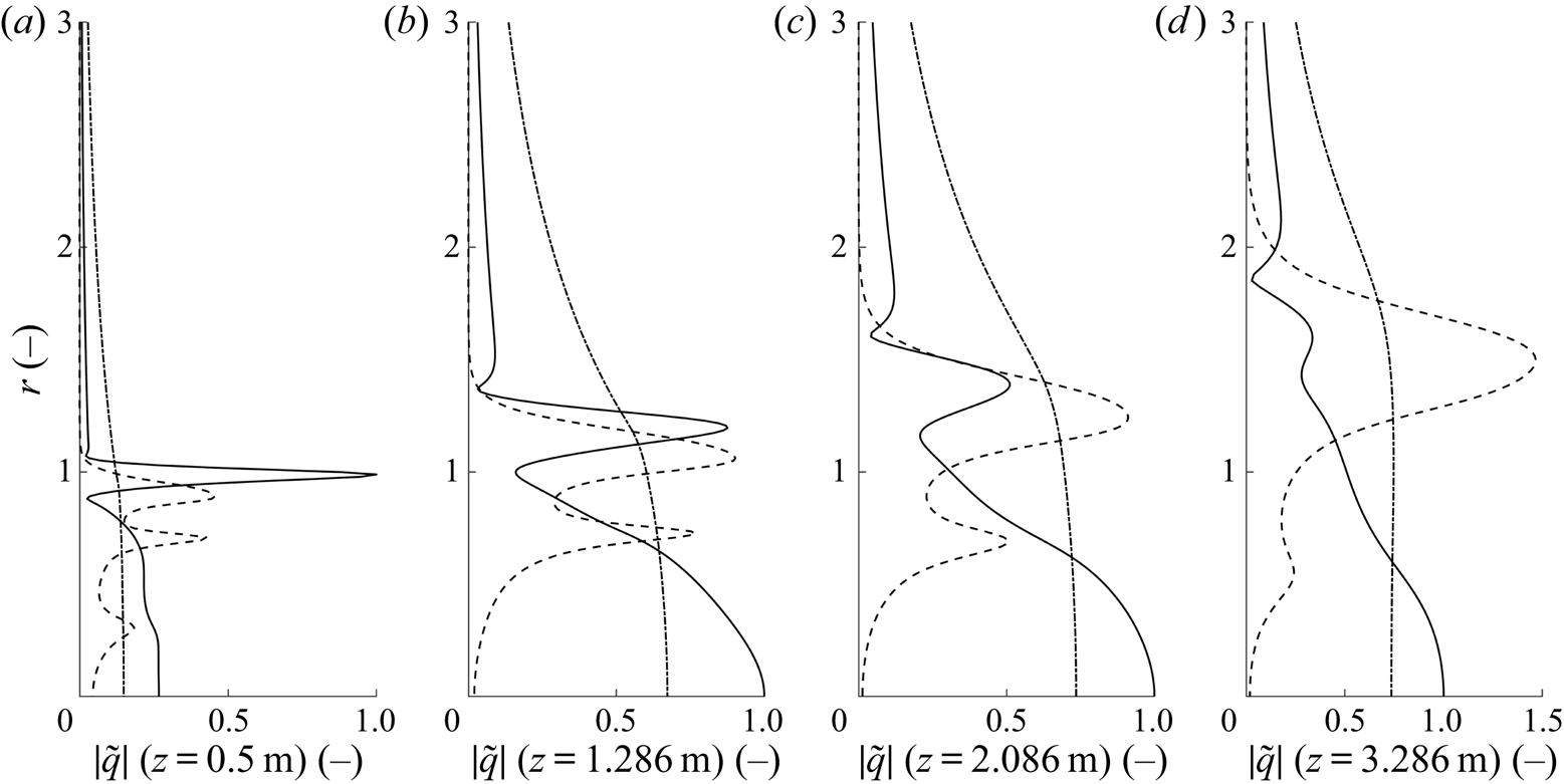
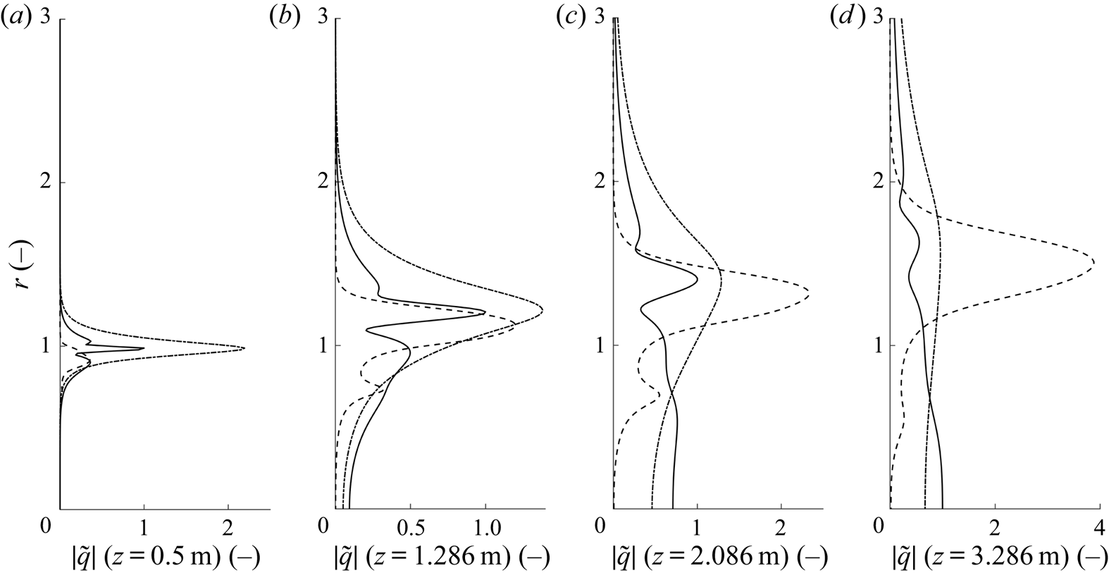
Shapes of the perturbations affiliated with  $S_0$ are given at four streamwise positions in figure 7. Saddle
 $S_0$ retains its mixed mode nature along the chamber as the pressure is amplified both at the centreline and shear layer, while the velocity perturbation becomes more amplified around the centreline as
 $z$ increases due to the decrease of secondary shear. As
 $z$ increases and the centreline temperature decreases, fewer dissociation reactions occur in the flow, which is seen by the vanishing number of peaks in the temperature perturbations. Finally, all perturbations are found to scale with the growing shear-layer thickness of the jet. Due to the extended length of the absolute region, the plasma jet should support a global mode (Lesshafft et al. Reference Lesshafft, Huerre, Sagaut and Terracol2006; Coenen & Sevilla Reference Coenen and Sevilla2012).
Magnitude of the axisymmetric perturbation functions corresponding to saddle  $S_0$ at 4 streamwise positions for the test case 5. The perturbation variables are respectively
 $\tilde {w}$ (
 $-$),
 $\tilde {T}$ (- -) and
 $\tilde {p}$ (
 ), and are normalized by
 $\max (|\tilde {w}|)$ at each position.

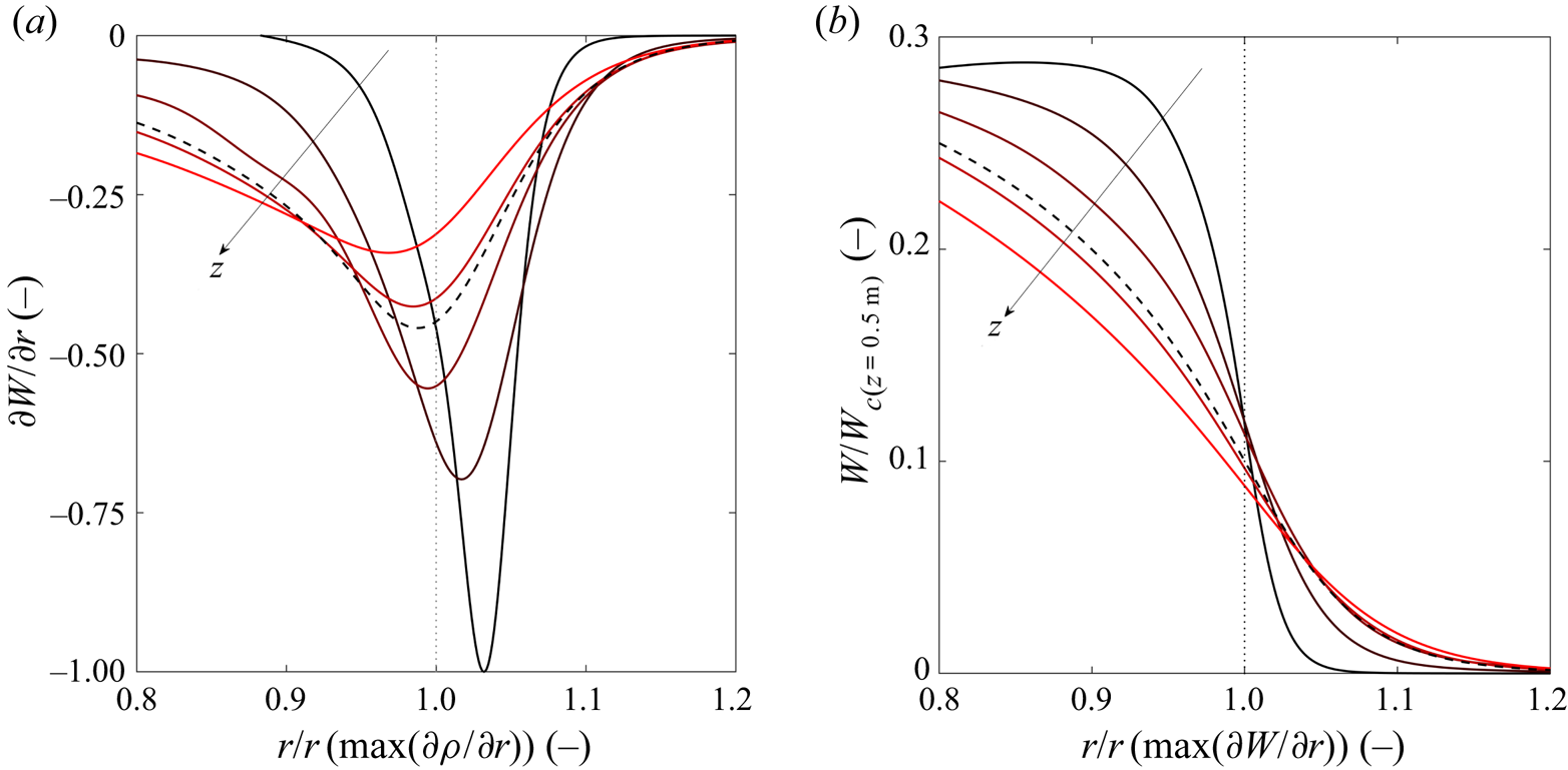
In order to explain the non-monotonic behaviour of the absolute growth rate with respect to  $z$, we recall two possible sources of absolute instabilities in jets: the baroclinic torque in heated jets (Lesshafft & Huerre Reference Lesshafft and Huerre2007) and the displacement of the maximum shear towards the low velocity areas (Lesshafft & Marquet Reference Lesshafft and Marquet2010). To promote the former, the positions of the maximum radial density gradient and maximum shear should be close to each other. However, the latter is also able to promote absolute instabilities even in the absence of baroclinic torque by reducing the group velocity at the maximum perturbation location. In the current cases, these two effects are in competition due to the specific shape of the plasma jet. As illustrated in figure 8(a), the velocity and density gradients are not aligned at the inlet but get closer as
 $z$ is increased, crossing each other around
 $z=0.92\ \textrm {m}$ and splitting further downstream. Accordingly, the absolute growth rate initially increases with
 $z$. However, its maximum value is reached beyond the position where the shears are aligned. The authors believe this offset to be due to the lower velocity at the maximum shear, observed as
 $z$ increases further. This is illustrated in figure 8(b), focusing on the secondary shear layer of the jet, where the velocity perturbation associated with
 $S_0$ is maximum. Moreover, the local velocity profiles of Plasmatron around
 $z=1\ \textrm {m}$ resemble greatly the profiles maximizing absolute instabilities obtained by Lesshafft & Marquet (Reference Lesshafft and Marquet2010). Further downstream, the absolute growth rate decreases while the Reynolds number, temperature ratio and shear-layer thickness all increase and
 $S$ remains of order
 $0.1$, in agreement with Lesshafft & Huerre (Reference Lesshafft and Huerre2007).
Evolution of the alignment between the maximum shear and maximum density gradient (a) and evolution of the velocity profiles around the maximum shear location (b) along  $z$ for case
 $5$. Profiles (solid lines) are given from
 $z=0.5\ \textrm {m}$ (dark) to
 $z=1.5\ \textrm {m}$ (light). The profiles are normalized by their maximum value at the inlet (see table 1 for velocity). The thick dashed line represents the profiles at maximum growth rate. The radial coordinate is normalized by the location where
 $\partial \rho /\partial r$ is maximum (a) and where
 $\partial W/\partial r$ is maximum (b) for each
 $z$ (thin dotted line).

However, jets with thick shear layers, characterized by  $R/\theta <5$ where
 $\theta$ is the momentum thickness, remain convectively unstable when considering simplified TTP models according to Lesshafft & Huerre (Reference Lesshafft and Huerre2007). In order to explain why the present jet is still absolutely unstable at
 $z=3.086\ \textrm {m}$, we consider the stability of the analytical jet defined by
 \begin{gather} \bar{w}=\frac{1}{2}\left(1 + \tanh\left[\frac{R}{4\theta} \left(\frac{1}{r} -r \right) \right] \right); \end{gather}
 \begin{gather}\bar{h} = S_h + \frac{1-S_h}{2}\left(1 + \tanh\left[\frac{R}{4\theta} \left(\frac{1}{r-d} -r +d \right) \right] \right); \end{gather}
adapted from (3.1a) and (3.1b) given by Lesshafft & Marquet (Reference Lesshafft and Marquet2010). Original profile equations from Lesshafft & Marquet (Reference Lesshafft and Marquet2010) are adapted to high temperatures by imposing a static enthalpy profile rather than a temperature one. The temperature profile, the ambient-to-centreline enthalpy ratio  $S_h = h_{\infty }/h_c$ obtained from
 $S$, and flow properties are reconstructed assuming LTE. The following values are used to approximate the plasma jet:
 $Re=250$,
 $R/\theta =4$,
 $S_h=0.0353$ (corresponding to
 $S=0.0715$),
 $M=0.0364$ and a radial offset of
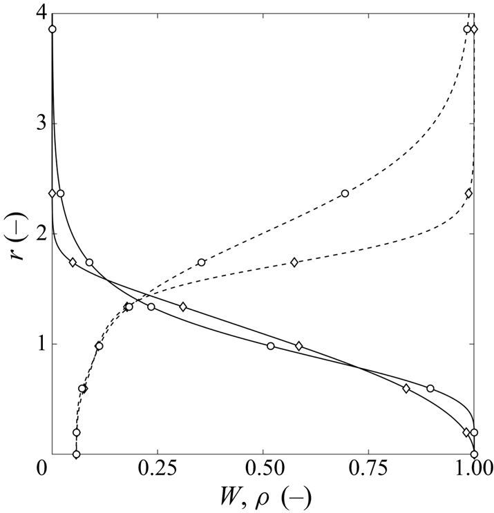
 $d=0.125$ between the velocity and enthalpy shears. Resulting profiles are compared to the present jet in figure 9 in terms of velocity and density. The significant offset observed between the density profiles is partly due to the greater sensitivity of the density to low temperatures. By tracking absolute instabilities along
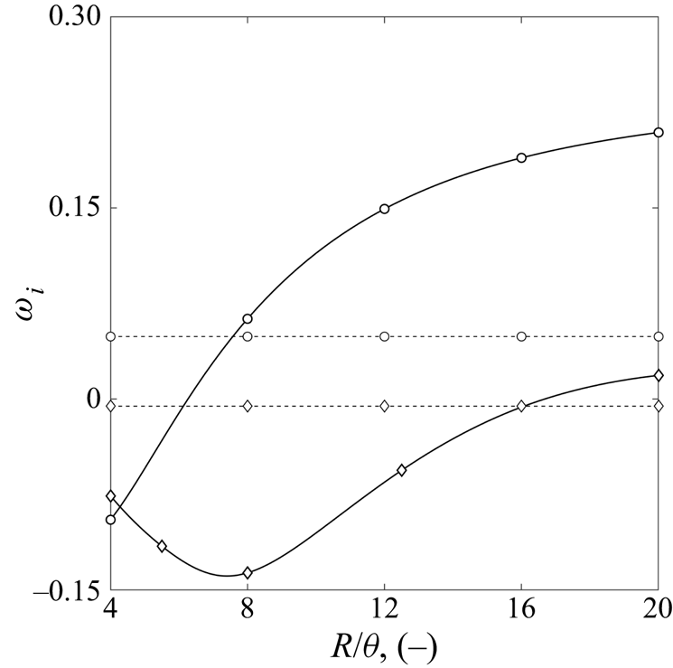
 $R/\theta =[20; 4]$, we find that for an equivalent jet thickness, the model adapted from Lesshafft & Marquet (Reference Lesshafft and Marquet2010) predicts a convectively unstable jet as plotted in figure 10. This indicates that the absolute nature of the thick shear-layer jet is not promoted by LTE effects, but is rather caused by the specific non-symmetric shape of the profiles, in agreement with conclusions from Lesshafft & Marquet (Reference Lesshafft and Marquet2010).
Comparison of the velocity ( $-$) and density (
 ) profiles of Plasmatron (
 ) against the adapted top-hat jet (
 ). Density is scaled with
 $\rho _{\infty }$ for plotting purposes.

Top-hat jet absolute growth-rate evolution with  $R/\theta$ for
 $m=0$ (
 ) and
 $m=1$ (
 ); and Plasmatron absolute growth rates at
 $z=3.086$ m (
 ).

Helical modes are also studied along the chamber by imposing  $m=[1,2]$. The streamwise evolution of the
 $m=1$ mode is plotted in figure 6(a), the
 $m=2$ mode is not plotted as its absolute growth rate remains below zero along the chamber. A region of absolute instability exists for the first helical mode and is contained inside the domain between
 $z=0.918$ and
 $z=2.838\ \textrm {m}$. The frequency at the start of the absolute region is
 $f=56.8\ \textrm {Hz}$ for
 $m=1$. In agreement with the conclusions of Lesshafft & Huerre (Reference Lesshafft and Huerre2007) for top hat jets in CPG, the absolute growth rate of helical mode remains smaller than the that of axisymmetric modes along the jet. The use of the jet model adapted from Lesshafft & Marquet (Reference Lesshafft and Marquet2010) also underestimates the absolute growth rate of the
 $m=1$ mode, as plotted in figure 10. Although not plotted, perturbation shapes of the first helical mode are similar to the axisymmetric ones, with the exception of the vanishing components of
 $\tilde {w}$,
 $\tilde {T}$,
 $\tilde {p}$ at the centreline imposed by the boundary conditions.
Assuming CPG properties and stability equations over-estimate both the absolute growth rate and frequency; as expected, the difference with respect to the LTE results is larger near the inlet of the test chamber, where the temperature is the highest. At the inlet, the CPG model over-estimates the growth rate by  $21\,\%$ and the absolute frequency by
 $57\,\%$ of the LTE values for
 $m=0$. An interesting observation is that the CPG absolute growth rate evolves with the same qualitative trends as for the LTE case, despite ignoring the high temperature effects on the flow properties and therefore on the non-dimensional numbers. At high temperatures (
 $T>9000\ \textrm {K}$ at
 $P_s=150\ \textrm {mbar}$), the viscosity behaviour with respect to temperature of a gas in LTE is inverted due to the presence of electrons. Consequently, the Reynolds number is found to decrease with
 $z$ from the inlet until
 $T_c <9000\ \textrm {K}$, where it starts to increase. This confirms the importance of studying the shapes described by velocity and density profiles, rather than only considering non-dimensional numbers.
4. Influence of the driving parameters
Unlike most of the studies in the literature, the present jet is controlled by the facility's driving parameters rather than imposing non-dimensional numbers independently. The effect of the driving parameters on the stability is investigated by varying the power and pressure around the values of  $P_{el}=100\ \textrm {kW}$ and
 $P_s=150\ \textrm {mbar}$ presented in the previous sections. A summary of all cases covered is given in table 1.
For all conditions, the first helical mode displays a lower absolute growth rate than the axisymmetric mode and it is not considered in the present section. For all cases, the contours of absolute growth rate remain qualitatively similar to the ones presented in figure 5, and the absolute mode at  $S_0$ remains the leading mode throughout the domain. Similarly, the trends of growth rate and frequency with the streamwise position associated with the saddle
 $S_0$ are similar to those shown in figure 6 for each case studied. For most cases, the region of absolute instability still extends beyond the end of the domain investigated, with the exception of the high power settings (
 $P_{el}=150\ \textrm {kW}$).
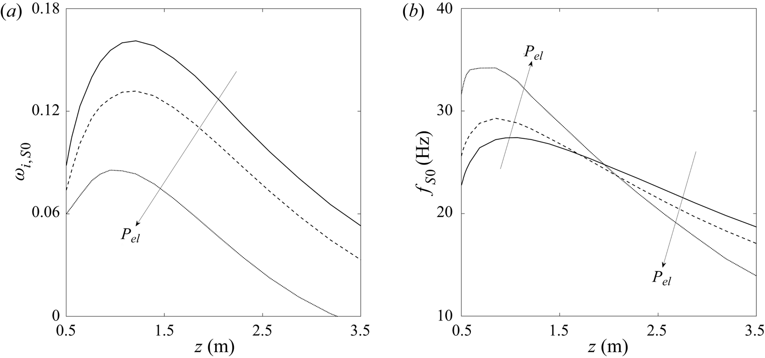
The influence of the power  $P_{el}$ on the evolution of the absolute growth rate and frequency along the chamber is displayed in figure 11 for a pressure fixed to
 $P_s=150\ \textrm {mbar}$. Increasing the power is found to uniformly reduce the amplification of the absolute instability throughout the chamber. This trend is in agreement with the increase of the inlet Mach number with power, known to dampen absolute instabilities (Lesshafft & Huerre Reference Lesshafft and Huerre2007). However, it conflicts with the increasing Reynolds number and decreasing temperature ratio, which should promote absolute instabilities. This last observation seems to indicate that the shape of local profiles defined by key non-dimensional numbers could be more important than the temperature ratio alone, and is analysed in more detail later on. Although the behaviour of the absolute frequency with the changes in power depends on the streamwise position, the maximum and initial frequencies increase with an increase of power while the opposite is observed in the second half of the chamber.
Influence of the electrical power on the streamwise evolution of the absolute growth rate (a) and frequency (b) associated with  $S_0$, for axisymmetric
 $m=0$ modes,
 $P_{el}=80\ \textrm {kW}$ (
 $-$),
 $P_{el}=100\ \textrm {kW}$ (- -) and
 $P_{el}=150\ \textrm {kW}$ (
 ) while
 $P_s=150\ \textrm {mbar}$.

The influence of the static pressure  $P_s$ on the absolute instabilities is displayed in figure 12, while the power is kept to
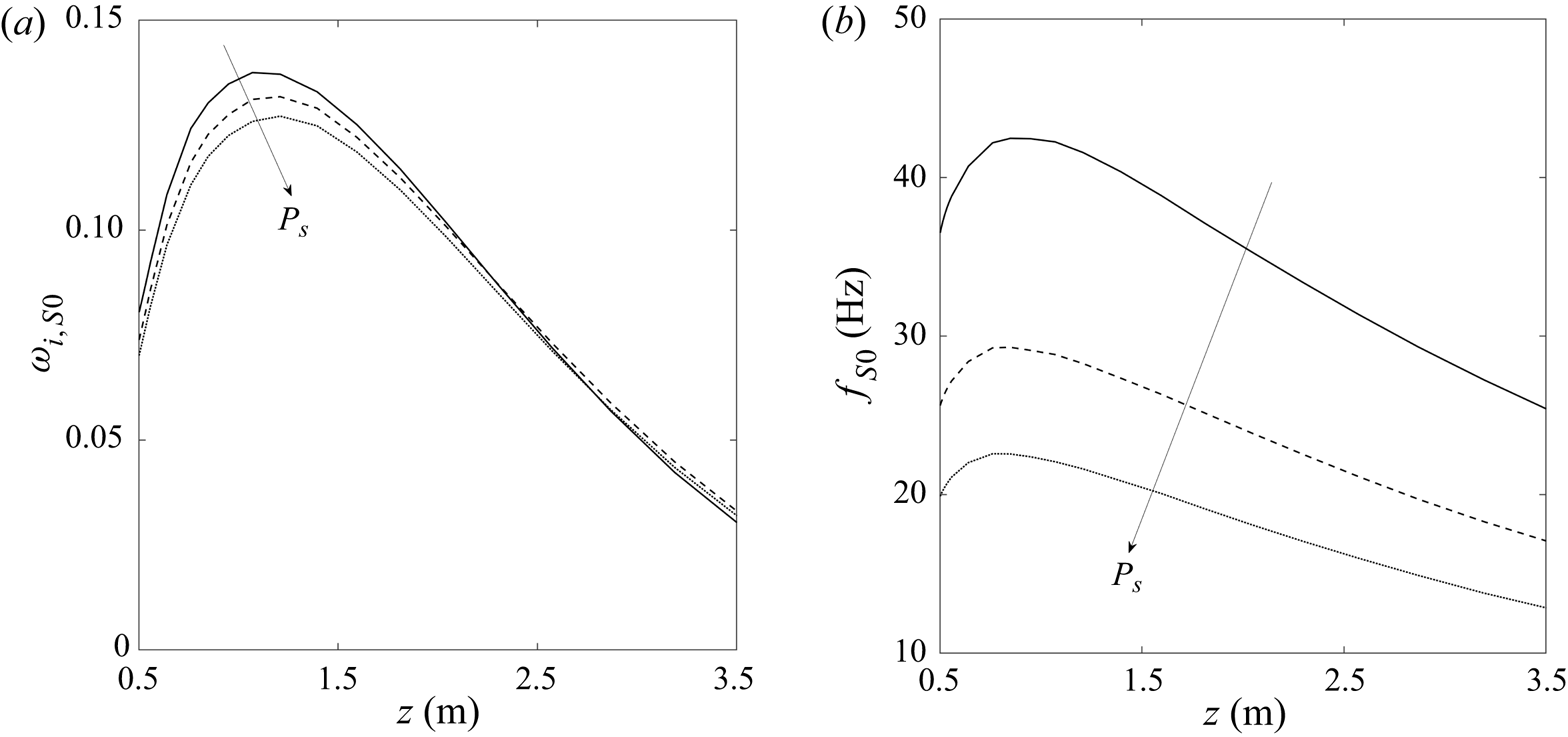
 $P_{el}=100\ \textrm {kW}$. From figure 12(a), it appears that the pressure has a limited adverse influence on
 $\sigma _{S0}$ throughout the chamber. On the other hand, pressure variations have a strong influence on the absolute frequency, which decreases when pressure is increased. Unlike the power, pressure influences the frequency qualitatively in the same way throughout the whole test chamber.
Influence of the chamber pressure on the streamwise evolution of the absolute growth rate (a) and frequency (b) associated with  $S_0$, for axisymmetric
 $m=0$ modes,
 $P_s=80\ \textrm {mbar}$ (
 $-$),
 $P_s=100\ \textrm {mbar}$ (- -) and
 $P_s=150\ \textrm {mbar}$ (
 ) at
 $P_{el}=100\ \textrm {kW}$.

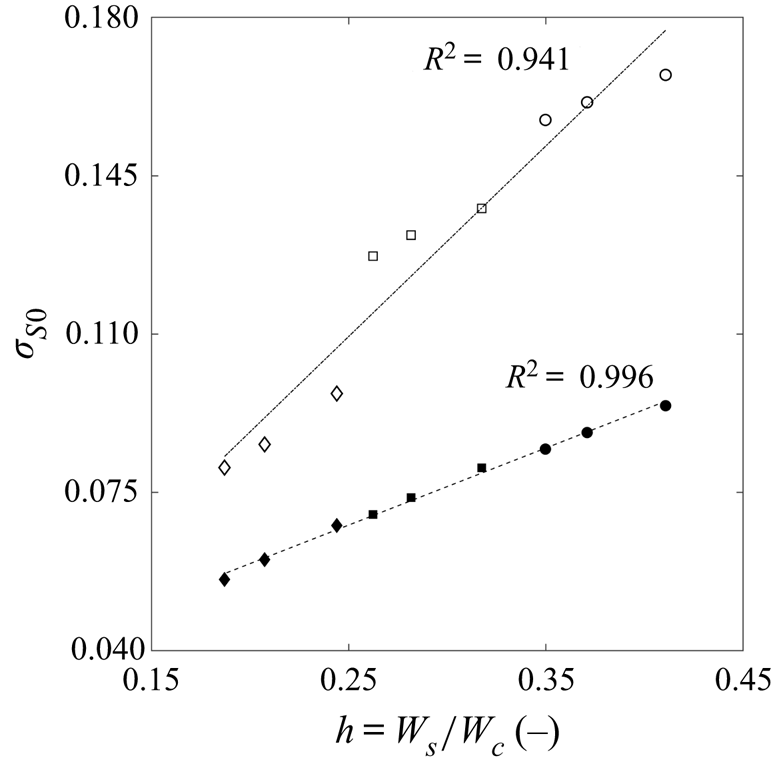
We observe that the absolute growth rate at the inlet depends linearly on the shape of the velocity profiles at the same position. Figure 13 shows this relation for which the regression  $\sigma _{S0}(z=0.5\,\textrm {m})=0.1704\times h_0+0.2518$ holds with a small variance indicated by
 ${R}^2=0.996$ when considering the cases of table 1. A similar scaling is found between the maximum
 $\sigma _{S0}$ along the chamber and the inlet bypass ratio, given by
 ${\rm max}({\sigma _{S0}})=0.4215\times h_0+0.0041$. As seen in figure 13, this correlation is less accurate than at the inlet, as
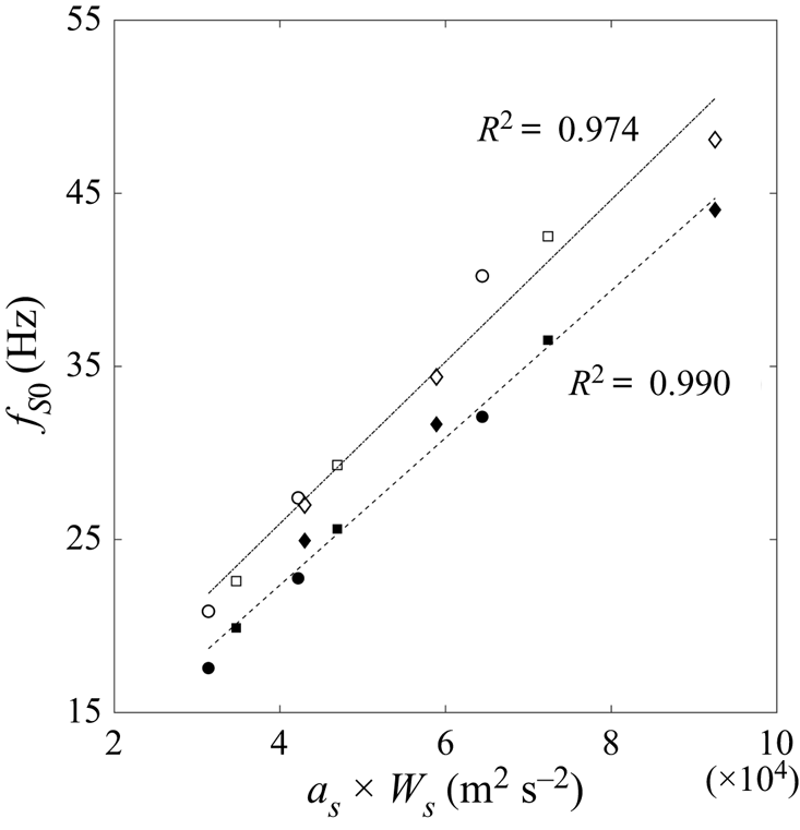
 $\text {R}^2=0.941$ in this case. However, this last result is particularly interesting as the growth rate of a linear global mode growing in the flow is bounded by the maximum local absolute growth rate (Chomaz, Huerre & Redekopp Reference Chomaz, Huerre and Redekopp1991). On the other hand, the absolute frequency at the inlet seems to be most significantly influenced by the pressure. Bearing in mind that the power mainly influences the bypass ratio but not the secondary shear-layer velocity, and that pressure mostly influences the values of velocity with a lesser influence on the bypass ratio, it can be assumed that the frequency depends on the secondary shear velocity
 $W_s$ at the inlet. Accordingly, the inlet frequency is found to scale linearly with
 $a_s\times W_s$ as plotted in figure 14,
 $a_s$ being the equilibrium speed of sound in the secondary shear at the inlet. The adjusted value of
 $R^2$ for the regression of frequency is of the same order as for the growth rate. A scaling is also found for the maximum value of the frequency and is plotted in figure 14. Similarly to the growth rate, this second scaling is less precise than for the inlet.
Correlations between inlet ( ) and maximum (
 $-$) absolute growth rates with respect to inlet bypass ratio for each case of table 1.

Correlations between inlet ( ) and maximum (
 $-$) absolute frequencies with respect to
 $a_s\times W_s$ at the inlet for each case of table 1.

Consistent with the results presented in § 3.2, the maximum growth-rate position remains located shortly downstream of the position where the maximum shear coincides with the maximum density gradient. No correlation is found between those two positions considering all cases, which could be due to the competition between the different effects discussed in the previous section.
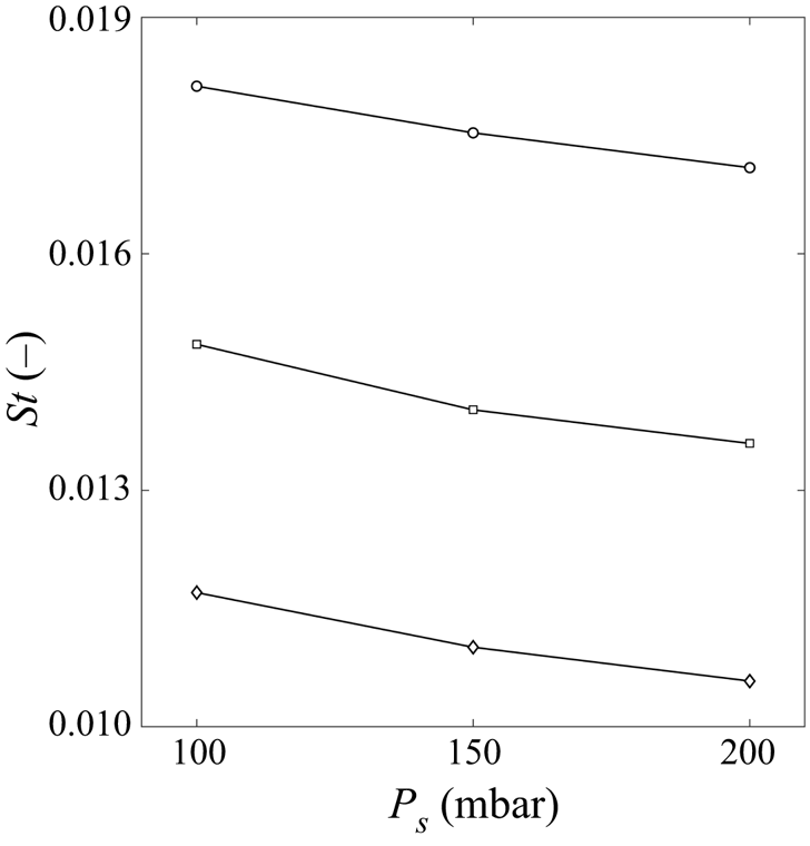
Experimental observations of Cipullo et al. (Reference Cipullo, Helber, Panerai, Zeni and Chazot2014) noted the leading role of the static pressure on the frequency of the oscillations recorded, which is in agreement with the present results. Furthermore, Cipullo et al. (Reference Cipullo, Helber, Panerai, Zeni and Chazot2014) assumed that the Strouhal number of the oscillations  $St=fl_{ref}/W_{c}$ remains constant with respect to pressure. The present calculations (figure 15) are in good agreement with this prediction, although a relatively small dependence on pressure is observed, possibly linked to the breakdown of the CPG assumption used by Cipullo.
Inlet absolute Strouhal number with respect to pressure at  $P_{el}=80\ \textrm {kW}$ (
 ),
 $P_{el}=100\ \textrm {kW}$ (
 ) and
 $P_{el}=150\ \textrm {kW}$ (
 ).

5. Full impulse response
The full impulse response of the wavepacket in the aftermath of a localized impulse is studied, using a method similar to Lesshafft & Huerre (Reference Lesshafft and Huerre2007). The extension of the previous results enables us to consider the competition between the absolute and convective instabilities supported by the flow. Non-zero values of the group velocity are imposed by shifting the reference frame, therefore modifying the non-dimensional streamwise velocity profile:  $W(v_{{g}})=W(v_{{g}}=0) - v_{{g}}$. Parameters of the travelling instabilities are then brought back into the static reference frame:
 $\sigma _{static}=\textrm {Im}(\omega _i(v_{{g}}))$ for the growth rate,
 $\alpha _{static}=\alpha (v_{{g}})$ for the complex wavenumber, and
 $\textrm {Re}(\omega _{static})=\omega _r(v_{{g}})+\alpha _r(v_{{g}})v_{{g}}$ for the real part of the frequency. Sweepings of the group velocity are calculated at four discrete locations along the test chamber for axisymmetric and first helical perturbations assuming a flow in LTE.
Results for the test case  $5$ of table 1 are plotted in figure 16 in terms of growth rate and real frequency. Due to changes in the profile shapes when increasing the streamwise position, two distinct behaviours of the full impulse response are observed along the chamber. In the first half of the chamber (
 $z=0.5\ \textrm {m}$ and
 $z=1.286\ \textrm {m}$) a competition mechanism, similar to the one described by Lesshafft & Huerre (Reference Lesshafft and Huerre2007) in top-hat jets with thin shear layers, involves two saddle points dominating at different group velocities. At null to low
 $v_{{g}}$, the absolute instability associated with saddle
 $S_0$ dominates the response. However, by increasing the group velocity the growth rate associated with a secondary saddle point becomes larger than the one of
 $S_0$, which is seen in figure 16 where discontinuities appear in the curves of growth rate and frequency. These secondary saddles are respectively
 $S_5$ at
 $z=0.5\ \textrm {m}$ (see figure 5a) and
 $S_1$ at
 $z=1.286\ \textrm {m}$ (see figure 5b). As their growth rate is negative for
 $v_{{g}}=0$, these saddles represent convective instabilities triggered by the impulse. Curves of the convective instabilities growth rate in figure 16(a) describe bell shapes reaching their maximum around
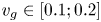 $v_{{g}}\in [0.1;0.2]$, which is lower than what can be observed in top-hat jets (Lesshafft & Huerre Reference Lesshafft and Huerre2007). Interestingly, while increasing
 $v_{{g}}$
 $S_0$ remains in the same area of the complex wavenumber plane, while
 $S_5$ and
 $S_1$ move towards the upper wavenumber plane (
 $\textrm {Im}(\alpha )>0$). Hence, we find that the saddle
 $S_0$ is no longer valid from the Briggs–Bers criterion point of view after the peak of growth rate observed in figure 16(a). One can also note that the convective instabilities maximum growth rate is reached while the corresponding saddle crosses the real wavenumber axis, in agreement with results from the temporal LST. The nature of convective instabilities is identified by plotting their associated shapes at maximum amplifications in figure 17. Both
 $S_5$ and
 $S_1$ exhibit typical shear-layer mode perturbation functions, featuring a maximum amplitude aligned with the maximum shear found in the secondary shear layer of the jet, and a vanishing component at the centreline. First azimuthal modes show a behaviour almost identical to the axisymmetric modes, except with a growth rate slightly lower than for
 $m=0$. Furthermore, the perturbation shapes associated with
 $m=1$ are similar to the ones of
 $m=0$ modes.
Spatio-temporal growth rate (a) and real part of the frequency (b) of the full impulse response for case 5, at  $z=0.5\ \textrm {m}$ (
 ),
 $z=1.286\ \textrm {m}$ (
 ),
 $z=2.086\ \textrm {m}$ (
 ) and
 $z=3.286\ \textrm {m}$ (
 $\ast$) for
 $m=0$ (
 $-$) and
 $m=1$ (- -).

Magnitude of perturbation functions corresponding to the most amplified saddle from the full impulse response for  $m=0$ and 4 streamwise positions of test case 5. The perturbation variables are respectively
 $\tilde {w}$ (
 $-$),
 $\tilde {T}$ (- -) and
 $\tilde {p}$ (
 ), and are normalized by
 $\max (|\tilde {w}|)$ at each position.

In the second half of the chamber ( $z=2.086$ and
 $z=3.286\ \textrm {m}$), no discontinuities are observed in the curves of
 $\omega (v_{{g}})$ as no valid secondary saddle point is found. Instead, the growth rates associated with
 $S_0$, and plotted in figure 16(a), describe the same bell shapes as the ones observed for
 $S_5$ and
 $S_1$ upstream. Additionally, saddle
 $S_0$ moves toward positive complex wavenumbers with increasing
 $v_{{g}}$ instead of remaining confined to the negative complex wavenumbers. The maximum growth rate is reached when
 $S_0$ crosses the
 $\alpha _i=0$ axis, similarly to convective instabilities associated with
 $S_5$ and
 $S_1$. Although the instabilities associated with
 $S_0$ have an absolute nature, they seem to behave similarly to convective instabilities in the second half of the jet. This can be explained by the perturbation shapes associated with
 $S_0$ at
 $v_{{g}}$ promoting the maximum amplification in figure 17. Shapes are now closer to shear-layer modes, with a maximum amplification near the maximum shear, but retain a significant component at the centreline, similarly to mixed modes in thick shear-layer jets (Lesshafft & Huerre Reference Lesshafft and Huerre2007). The first helical modes behave similarly to the axisymmetric modes, although their maximum amplification is reached for higher values of
 $v_{{g}}$. Furthermore, their maximum amplification at
 $z=3.286\ \textrm {m}$ is higher than for the
 $m=0$ modes, which is in agreement with the observations of Lesshafft et al. (Reference Lesshafft, Huerre and Sagaut2007) for jets with thick shear layers. Mode shapes for
 $m=1$ are also similar to the
 $m=0$ shapes for this part of the jet, even though perturbations vanish at the centreline due to the boundary conditions.
Unlike the absolute growth rate studied in the previous section, the maximum value of  $\sigma (v_{{g}})$ decreases monotonously along the streamwise direction.
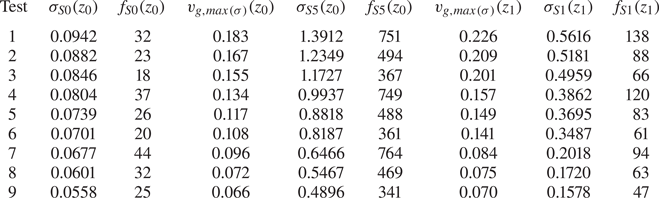
Variations of the driving parameters in the range of table 1 do not significantly alter the behaviour of the full impulse response. Decreasing both the power and pressure increases the length of the jet for which the competition between saddles is observed; for the case  $1$ (80 kW and 100 mbar), this region extends to
 $z=2.086\ \textrm {m}$. Results of the full impulse response are given for each case in table 2 in terms of dimensional frequency and growth rate for
 $m=0$. Increasing the electric power increases the first helical modes beyond the
 $m=0$ modes in the second part of the jet. The maximum growth rate of the full impulse response behaves similarly to the one of absolute instabilities with respect to the driving parameters. Furthermore, the maximum convective growth rate of axisymmetric modes at the inlet scales linearly with the absolute growth rate, and thus with the inlet bypass ratio
 $h_{{b}}$. Contrary to the absolute frequency, the maximum frequency of convective instabilities decreases when increasing
 $P_{el}$. This last observation contradicts the experimental trends of Cipullo et al. (Reference Cipullo, Helber, Panerai, Zeni and Chazot2014), which seem to agree with the predominant role of the absolute instabilities in the flow.
Results of the full impulse response for the test cases defined in table 2. The growth rate and dimensional frequencies (in Hz) for saddles  $S_5$ and
 $S_1$ are given for the group velocity at maximum amplification. The streamwise positions are noted
 $z_0 = 0.5$ and
 $z_1=1.286\ \textrm {m}$.

6. Conclusions
The spatio-temporal LST analysis of a plasma jet based on the VKI Plasmatron has been performed for the first time. The flow is assumed to be a mixture of gases in LTE both in the base state and the stability equations.
A first detailed analysis has been carried out by maintaining the electric power at  $P_{el}=100\ \textrm {kW}$, the static pressure at
 $P_s=150\ \textrm {mbar}$ and the mass flow at
 $\dot {m}_{air}=16\ \textrm {g}\ \textrm {s}^{-1}$. This analysis revealed the presence of an unexpectedly extended region of absolute instability in the flow, starting at the inlet of the chamber, not represented in earlier studies. This result is obtained considering axisymmetric perturbations, and the mode at the start of this region displays shapes similar to the outer modes in CPG co-axial jets described by Balestra et al. (Reference Balestra, Gloor and Kleiser2015). Further downstream, the absolute mode takes the shape of mixed modes described by Lesshafft & Huerre (Reference Lesshafft and Huerre2007) in top hat jets with thick shear layers. Its associated growth rate exhibits a non-monotonic behaviour along the streamwise direction, peaking around an intermediate position downstream of the inlet. This behaviour has been related to the competition between two effects promoting absolute instabilities documented in the literature: on the one hand the baroclinic torque caused by the alignment of the shear and density layers (Lesshafft & Huerre Reference Lesshafft and Huerre2007), and on the other hand the displacement of the maximum shear towards low velocity regions of the jet by seemingly lowering the group velocity (Lesshafft & Marquet Reference Lesshafft and Marquet2010). Such arguments are in line with previous observations (Coenen et al. Reference Coenen, Sevilla and Sanchez2008; Coenen & Sevilla Reference Coenen and Sevilla2012) highlighting the importance of profile shapes in the study of realistic flows. This is further emphasized by the fact that the thick shear-layer Plasmatron jet near the outlet remains absolutely unstable, while top-hat jet profiles with similar parameters are convectively unstable.
A similar analysis with first helical modes  $m=1$ reveals a smaller pocket of absolute instability fully contained inside the domain. However, the growth rate of these modes is less than that of axisymmetric modes, in agreement with Monkewitz & Sohn (Reference Monkewitz and Sohn1988).
CPG thermo-transport properties and stability equations for the same base state significantly over-estimate both the growth rate and frequency of the absolute instabilities in the jet, even though the stability features remain qualitatively similar when considering chemical reactions in equilibrium.
The complex nature of the flow does not allow a simple parameter sweep as commonly found in the literature; accordingly, the influence of the VKI Plasmatron driving parameters on the stability features of the jet has been investigated. An increase of the electric power is found to mainly diminish the absolute growth rate, while increasing the pressure is found to chiefly dampen the dimensional absolute frequency. The reader is reminded that due to similar scales of the absolute wavelength and the development length of the flow at the inlet, a quantitative comparison between the frequencies of local absolute modes and global modes should not be attempted. However, the good agreement between experiments and trends of the absolute frequency with respect to Plasmatron driving parameters, suggest that a qualitative comparison is possible. This study confirmed the theoretical strong dependence of the inlet Strouhal number (based on the absolute frequency) on power, and the limited effect of pressure, as suggested by Cipullo et al. (Reference Cipullo, Helber, Panerai, Zeni and Chazot2014). The growth rate varies linearly with the bypass ratio at the inlet, while the dimensional frequency scales linearly with  $a_s W_s$. To the authors’ knowledge, such scaling has not been reported before in the literature, but may be linked to the specific profiles and flow parameters of the Plasmatron jet.
The complexity of the profiles studied, imposed by technological constraints in the facility, has been highlighted through the competition of different modes in the full impulse response. In the first half of the jet, with thin shear layers, a competition mechanism between jet-column absolute instabilities dominating at low group velocities, and shear-layer type convective instabilities taking over at higher velocities is observed. Further downstream, with thicker shear layer, a single saddle point of mixed mode nature dominates the impulse response. Both impulse responses are in good qualitative agreement with the observations of Lesshafft & Huerre (Reference Lesshafft and Huerre2007) for top hat jets with thin/thick shear layers. However, the frequency behaviour of convective instabilities with respect to changes of power conflicts with experimental observations. This suggests that absolute instabilities are responsible for the jet oscillations observed in the Plasmatron. Even though the plasma jet displays many unusual attributes with respect to the base states in the literature, its stability features are coherent with combinations of effects described in other studies for much lower temperature axisymmetric jets.
The present study found a large region of absolute instability which is expected to generate a global mode pulsating at the inlet absolute frequency. This hypothesis appears to be compatible with experimental observations reporting a single frequency in the flow (Cipullo et al. Reference Cipullo, Helber, Panerai, Zeni and Chazot2014), but cannot be verified due to the limiting capabilities of the one-dimensional LST. However, the recent work of Coenen et al. (Reference Coenen, Lesshafft, Garnaud and Sevilla2017) and the ideas presented previously suggests that a streamwise biglobal stability study should yield more precise results in terms of frequency, and presents a promising perspective that deserves further developments.
Acknowledgements
This work benefited from the support of the Belgian National Fund for Scientific Research under the FRIA Grant warrant (FNRS, dossier  $FC27631$).
Declaration of interests
The authors report no conflict of interest.
Appendix A
A.1. Analytical interpolation
Coefficients used for the analytical interpolation of the test case  $5$ defined in table 1 are given in table 4 for the velocity and table 5 for the temperature fields. Dimensional profiles are obtained by scaling back the radial coordinate by
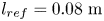 $l_{ref}=0.08\ \textrm {m}$ and applying the relations given in (A 1a) and (A 1b).
 \begin{gather} W_{dim} = W(r)W_c(z) \end{gather}
 \begin{gather}T_{dim} = T(r)\left(T_c(z) - T_{wall} \right) + T_{wall} . \end{gather}
Where the streamwise centreline velocity  $W_c(z)$ and temperature
 $T_c(z)$ are given in table 3 for the test case
 $5$ defined in table 1,
 $T_{wall}=350\ \textrm {K}$, and
 $W(r)$,
 $T(r)$ are defined in (2.2a) and (2.2b).
Centreline velocity and temperature along the test chamber for the  $P_{el} = 100$ kW and
 $P_s = 150$ mbar case.

The ability of the analytical model to reproduce the flow from simulations is showcased in figure 18 for the case with  $P_{el}=100\ \textrm {kW}$ and
 $P_s=150\ \textrm {mbar}$.
Comparison between the velocity (a) and temperature (b) profiles obtained from Plasmatron simulations ( ) against the analytical interpolations (
 ) used in the stability analysis. The profiles are given for the
 $P_{el}=100\ \textrm {kW}$ and
 $P_s=150\ \textrm {mbar}$ case, at the same streamwise positions than in tables 4 and 5.

Coefficients for analytical interpolation of streamwise velocity field of the  $P_{el} = 100$ kW and
 $P_s = 150$ mbar case.

Coefficients for analytical interpolation of temperature field of the  $P_{el} = 100$ kW and
 $P_s = 150$ mbar case.

A.2. Examples of plasma flow properties
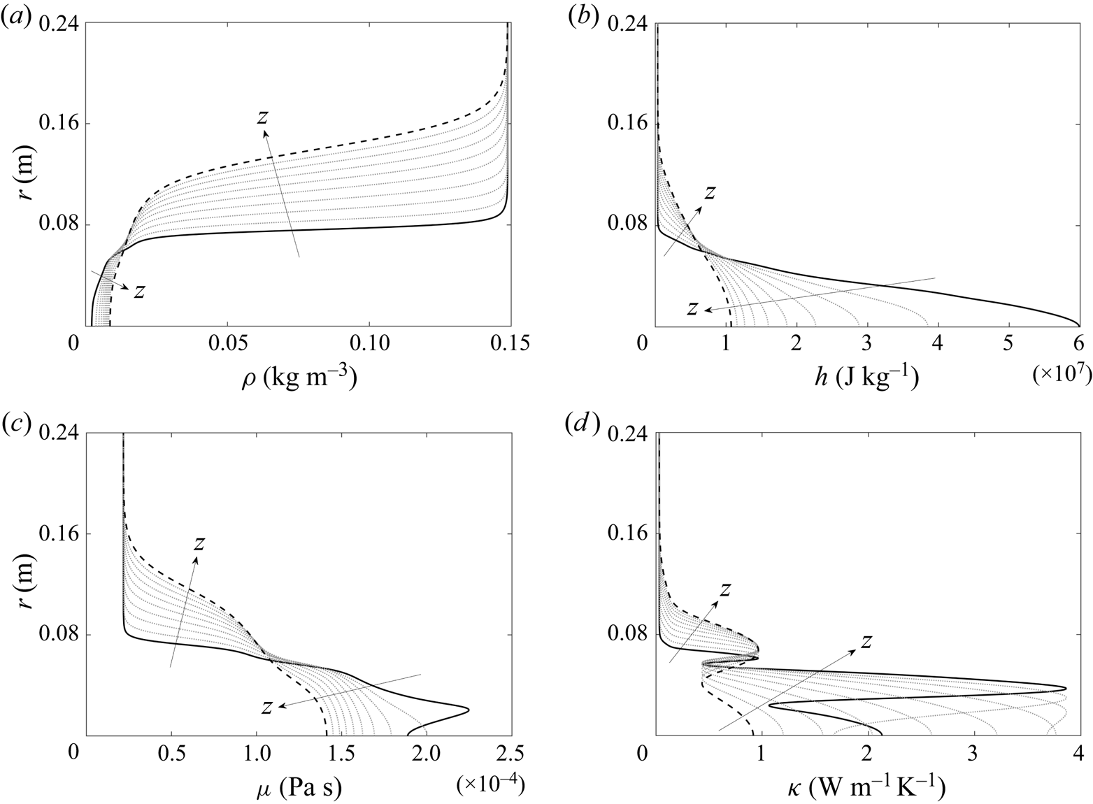
Additional profiles of the flow thermodynamic and transport properties along the test chamber are plotted in figure 19 for the test case 5 of table 1. The properties plotted are computed in the VESTA toolkit, based on the temperature distribution along the jet and the static pressure in the chamber. High temperature effects are particularly visible in the viscosity and thermal conductivity profiles, where the humps observed are due to changes of the equilibrium mixture composition. The strong damping effect of ionization on the viscosity is showcased near the centreline of the inlet profile in figure 19(c) where temperatures are above 9000 K.
Flow field quantities for the  $P_{el}=100\ \textrm {kW}$ and
 $P_s=150\ \textrm {mbar}$ case along the test chamber, from
 $z=0.5\ \textrm {m}$ (
 $-$) to
 $z=3.5\ \textrm {m}$ (- -), with intermediate profiles (
 ) linearly spaced between the inlet and outlet. (a) Density; (b) static enthalpy; (c) dynamic viscosity; and (d) thermal conductivity.

Appendix B
B.1. Stability equations
Stability equations described with the cylindrical coordinates are derived automatically (Pinna & Groot Reference Pinna and Groot2014) within the ADIT module of the VESTA toolkit, assuming a flow in LTE. The temporal eigenvalue problem is of the form  $(A+B\omega )\tilde {q}=0$, where
 $\tilde {q}=[\tilde {u},\tilde {v}, \tilde {w},\tilde {T},\tilde {p}]$ and the
 $A$ and
 $B$ matrices are given as
 \begin{align} A &= \left[ \begin{array}{@{}ccccc@{}} ~A_{1\times1} & ~A_{1\times2} & ~A_{1\times3} & ~A_{1\times4} & ~A_{1\times5} \\ ~A_{2\times1} & ~A_{2\times2} & ~A_{2\times3} & ~A_{2\times4} & ~A_{2\times5} \\ ~A_{3\times1} & ~A_{3\times2} & ~A_{3\times3} & ~A_{3\times4} & ~A_{3\times5} \\ ~A_{4\times1} & ~A_{4\times2} & ~A_{4\times3} & ~A_{4\times4} & ~A_{4\times5} \\ ~A_{5\times1} & ~A_{5\times2} & ~A_{5\times3} & ~A_{5\times4} & ~A_{5\times5} \end{array} \right],\nonumber\\ B &= \left[\begin{array}{@{}ccccc@{}} ~0 & ~0 & ~0 & ~B_{1\times4} & ~B_{1\times5} \\ ~B_{2\times1} & ~0 & ~0 & ~0 & ~0 \\ ~0 & ~B_{3\times2} & ~0 & ~0 & ~0 \\ ~0 & ~0 & ~B_{4\times3} & ~0 & ~0 \\ ~0 & ~0 & ~0 & ~B_{5\times4} & ~B_{5\times5} \end{array} \right], \end{align}
with sub-matrices of  $B$ defined as
 \begin{equation} \left.\begin{aligned} \boldsymbol{B_{1\times4}} = \frac{{\textrm{i}\bar{G}\bar{p}}}{{\bar{T}}};\quad \boldsymbol{B_{1\times5}} = -\textrm{i}\bar{F};\quad \boldsymbol{B_{2\times1}} = -\frac{{\textrm{i}\mathcal{H}\bar{p}}}{{\bar{T}\bar{\zeta}}};\quad \boldsymbol{B_{3\times2}} = -\frac{{\textrm{i}\mathcal{H}\bar{p}}}{{\bar{T}\bar{\zeta}}};\quad \\ \boldsymbol{B_{4\times3}} = -\frac{{\textrm{i}\mathcal{H}\bar{p}}}{{\bar{T}\bar{\zeta}}};\quad \boldsymbol{B_{5\times4}} = -\frac{{\textrm{i}\mathcal{H}\bar{\mathcal{H}}_{\bar{T}}\bar{p}}}{{\bar{T}\bar{\zeta}}};\quad \boldsymbol{B_{5\times5}} = \textrm{i}Ec-\frac{{\textrm{i}\mathcal{H}\bar{\mathcal{H}}_{\bar{p}}\bar{p}}}{{\bar{T}\bar{\zeta}}}, \end{aligned}\right\} \end{equation}
and sub-matrices of  $A$ defined as
 \begin{gather} \boldsymbol{A_{1\times1}} = \mathcal{D}_0\left(\frac{{\bar{p}}}{{r}}+\bar{F} \bar{p}_{r}-\frac{{\bar{G}\bar{T}_{r}\bar{p}}}{{\bar{T}}}\right)+\mathcal{D}_1\bar{p}, \end{gather}
 \begin{gather}\boldsymbol{A_{1\times2}} = \frac{{\textrm{i}\mathcal{D}_0m\bar{p}}}{{r}}, \end{gather}
 \begin{gather}\boldsymbol{A_{1\times3}} = \textrm{i}\mathcal{D}_0\alpha\bar{p}, \end{gather}
 \begin{gather}\boldsymbol{A_{1\times4}} = \mathcal{D}_0\left(-\frac{{\textrm{i}\bar{G}\bar{v}m \bar{p}}}{{\bar{T}r}}-\frac{{\textrm{i}\bar{G}\bar{w}\alpha\bar{p}}}{{\bar{T}}}\right), \end{gather}
 \begin{gather}\boldsymbol{A_{1\times5}} = \mathcal{D}_0\left(\frac{{\textrm{i}\bar{F}\bar{v}m}}{{r}}+\textrm{i}\bar{F}\bar{w}\alpha\right), \end{gather}
 \begin{align} \boldsymbol{A_{2\times1}} &= \mathcal{D}_0\left(-\frac{{\bar{\lambda}_{\bar{p}} \bar{p}_{r}}}{{{Re}\,r}}+\frac{{\textrm{i}\mathcal{H}\bar{v}m \bar{p}}}{{\bar{T}\bar{\zeta}r}}-\frac{{ \bar{T}_{r}\bar{\lambda}_{\bar{T}}}}{{{Re}\, r}}+\frac{{m^2\bar{\mu}}}{{{Re}\,r^2}}+\frac{{2 \bar{\mu}}}{{{Re}\,r^2}}+\frac{{\bar{\lambda}}}{{{Re}\,r^2}}+ \frac{{\textrm{i}\mathcal{H}\bar{w}\alpha\bar{p}}}{{\bar{T}\bar{\zeta}}}+ \frac{{\alpha^2\bar{\mu}}}{{{Re}}}\right) \nonumber\\ &\quad + \mathcal{D}_1\left(-\frac{{2\bar{\mu}}}{{{Re}\,r}}- \frac{{\bar{\lambda}}}{{{Re}\,r}}- \frac{{2\bar{\mu}_{\bar{p}}\bar{p}_{r}}}{{{Re}}}- \frac{{\bar{\lambda}_{\bar{p}}\bar{p}_{r}}}{{{Re}}} -\frac{{2\bar{T}_{r}\bar{\mu}_{\bar{T}}}}{{{Re}}}- \frac{{\bar{T}_{r}\bar{\lambda}_{\bar{T}}}}{{{Re}}}\right) \nonumber\\ &\quad + \mathcal{D}_2\left(-\frac{{2\bar{\mu}}}{{{Re}}}- \frac{{\bar{\lambda}}}{{{Re}}}\right), \end{align}
 \begin{align} \boldsymbol{A_{2\times2}} &= \mathcal{D}_0\left(-\frac{{\textrm{i}m\bar{\lambda}_{\bar{p}} \bar{p}_{r}}}{{{Re}\,r}}-\frac{{2\mathcal{H}\bar{v} \bar{p}}}{{\bar{T}\bar{\zeta}r}}-\frac{{\textrm{i} \bar{T}_{r}m\bar{\lambda}_{\bar{T}}}}{{{Re}\,r}}+ \frac{{3\textrm{i}m\bar{\mu}}}{{{Re}\,r^2}}+ \frac{{\textrm{i}m\bar{\lambda}}}{{{Re}\,r^2}}\right) \nonumber\\ &\quad + \mathcal{D}_1\left(-\frac{{\textrm{i}m\bar{\mu}}}{{{Re}\,r}}- \frac{{\textrm{i}m\bar{\lambda}}}{{{Re}\,r}}\right), \end{align}
 \begin{gather} \boldsymbol{A_{2\times3}} = \mathcal{D}_0\left(-\frac{{\textrm{i}\alpha\bar{\lambda}_{\bar{p}} \bar{p}_{r}}}{{{Re}}}-\frac{{\textrm{i}\bar{T}_{r}\alpha \bar{\lambda}_{\bar{T}}}}{{{Re}}}\right)+ \mathcal{D}_1\left(-\frac{{\textrm{i}\alpha\bar{\mu}}}{{{Re}}}- \frac{{\textrm{i}\alpha\bar{\lambda}}}{{{Re}}}\right), \end{gather}
 \begin{gather}\boldsymbol{A_{2\times4}} = \mathcal{D}_0\left(\frac{{\bar{G}\mathcal{H}\bar{v}^2\bar{p}}}{{\bar{T}^2 \bar{\zeta}r}}-\frac{{\textrm{i}\bar{v}_{r}m\bar{\mu}_{\bar{T}}}}{{{Re}\,r}}+\frac{{\textrm{i}\bar{v}m\bar{\mu}_{\bar{T}}}}{{{Re}\,r^2}}-\frac{{\textrm{i}\bar{w}_{r}\alpha\bar{\mu}_{\bar{T}} }}{{{Re}}}\right), \end{gather}
 \begin{equation}\boldsymbol{A_{2\times5}} = \mathcal{D}_0\left(-\frac{{\textrm{i}\bar{v}_{r}m\bar{\mu}_{\bar{p}}}}{{{Re}\,r}}- \frac{{\bar{F}\mathcal{H}\bar{v}^2}}{{\bar{T}\bar{\zeta}r}}+ \frac{{\textrm{i}\bar{v}m\bar{\mu}_{\bar{p}}}}{{{Re}\,r^2}}- \frac{{\textrm{i}\bar{w}_{r}\alpha\bar{\mu}_{\bar{p}}}}{{{Re}}}\right)+\mathcal{D}_1, \end{equation}
 \begin{align} \boldsymbol{A_{3\times1}} &= \mathcal{D}_0\left(-\frac{{\textrm{i}m\bar{\mu}_{\bar{p}} \bar{p}_{r}}}{{{Re}\,r}}+ \frac{{\mathcal{H}\bar{v}\bar{p}}}{{\bar{T}\bar{\zeta}r}}- \frac{{\textrm{i}\bar{T}_{r}m\bar{\mu}_{\bar{T}}}}{{{Re}\,r}}- \frac{{3\textrm{i}m\bar{\mu}}}{{{Re}\,r^2}}- \frac{{\textrm{i}m\bar{\lambda}}}{{{Re}\,r^2}}+ \frac{{\mathcal{H}\bar{v}_{r}\bar{p}}}{{\bar{T}\bar{\zeta}}}\right) \nonumber\\ &\quad + \mathcal{D}_1\left(-\frac{{\textrm{i}m\bar{\mu}}}{{{Re}\,r}}- \frac{{\textrm{i}m\bar{\lambda}}}{{{Re}\,r}}\right), \end{align}
 \begin{align} \boldsymbol{A_{3\times2}} &= \mathcal{D}_0 \left(\frac{{\bar{\mu}_{\bar{p}}\bar{p}_{r}}}{{{Re}\,r}}+ \frac{{\textrm{i}\mathcal{H}\bar{v}m\bar{p}}}{{\bar{T}\bar{\zeta}r}}+ \frac{{\bar{T}_{r} \bar{\mu}_{\bar{T}}}}{{{Re}\,r}}+ \frac{{2m^2\bar{\mu}}}{{{Re}\,r^2}}+ \frac{{\bar{\mu}}}{{{Re}\,r^2}}+\frac{{m^2\bar{\lambda}}}{{{Re}\,r^2}}+ \frac{{\textrm{i}\mathcal{H}\bar{w}\alpha\bar{p}}}{{\bar{T}\bar{\zeta}}}+ \frac{{\alpha^2\bar{\mu}}}{{{Re}}}\right) \nonumber\\ &\quad + \mathcal{D}_1\left(-\frac{{\bar{\mu}}}{{{Re}\,r}}- \frac{{\bar{\mu}_{\bar{p}}\bar{p}_{r}}}{{{Re}}}- \frac{{\bar{T}_{r}\bar{\mu}_{\bar{T}}}}{{{Re}}}\right)- \frac{{\mathcal{D}_2\bar{\mu}}}{{{Re}}}, \end{align}
 \begin{equation} \boldsymbol{A_{3\times3}} = \mathcal{D}_0\left(\frac{{\alpha m \bar{\mu}}}{{{Re}\,r}}+\frac{{\alpha m \bar{\lambda}}}{{{Re}\,r}}\right), \end{equation}
 \begin{align} \boldsymbol{A_{3\times4}} &= \mathcal{D}_0\left(\frac{{\bar{v}\bar{\mu}_{\bar{T} \bar{p}}\bar{p}_{r}}}{{{Re}\,r}}+\frac{{\bar{T}_{r} \bar{v}\bar{\mu}_{\bar{T}\bar{T}}}}{{{Re}\,r}}- \frac{{\bar{v}_{r}\bar{\mu}_{\bar{T}}}}{{{Re}\,r}}+ \frac{{\bar{v}\bar{\mu}_{\bar{T}}}}{{{Re}\,r^2}}- \frac{{\bar{v}_{r}\bar{\mu}_{\bar{T}\bar{p}}\bar{p}_{r}}}{{{Re}}}- \frac{{\bar{T}_{r}\bar{v}_{r}\bar{\mu}_{\bar{T}\bar{T}}}}{{{Re}}}- \frac{{\bar{v}_{rr}\bar{\mu}_{\bar{T}}}}{{{Re}}}\right) \nonumber\\ &\quad + \mathcal{D}_1\left(\frac{{\bar{v}\bar{\mu}_{\bar{T}}}}{{{Re}\,r}}- \frac{{\bar{v}_{r}\bar{\mu}_{\bar{T}}}}{{{Re}}}\right), \end{align}
 \begin{align} \boldsymbol{A_{3\times5}} &= \mathcal{D}_0\left(\frac{{\bar{v}\bar{\mu}_{\bar{p} \bar{p}}\bar{p}_{r}}}{{{Re}\,r}}- \frac{{\bar{v}_{r}\bar{\mu}_{\bar{p}}}}{{{Re}\,r}}+ \frac{{\bar{T}_{r}\bar{v}\bar{\mu}_{\bar{T}\bar{p}}}}{{{Re}\,r}}+ \frac{{\textrm{i}m}}{{r}}+\frac{{\bar{v}\bar{\mu}_{\bar{p}}}}{{{Re}\,r^2}}- \frac{{\bar{v}_{r}\bar{\mu}_{\bar{p}\bar{p}}\bar{p}_{r}}}{{{Re}}}- \frac{{\bar{v}_{rr}\bar{\mu}_{\bar{p}}}}{{{Re}}}- \frac{{\bar{T}_{r}\bar{v}_{r}\bar{\mu}_{\bar{T}\bar{p}}}}{{{Re}}}\right) \nonumber\\ &\quad + \mathcal{D}_1\left(\frac{{\bar{v}\bar{\mu}_{\bar{p}}}}{{{Re}\,r}}- \frac{{\bar{v}_{r}\bar{\mu}_{\bar{p}}}}{{{Re}}}\right), \end{align}
 \begin{gather} \boldsymbol{A_{4\times1}} = \mathcal{D}_0\left(-\frac{{\textrm{i}\alpha\bar{\mu}}}{{{Re}\,r}}- \frac{{\textrm{i}\alpha\bar{\lambda}}}{{{Re}\,r}}- \frac{{\textrm{i}\alpha \bar{\mu}_{\bar{p}}\bar{p}_{r}}}{{{Re}}}+ \frac{{\mathcal{H}\bar{w}_{r}\bar{p}}}{{\bar{T}\bar{\zeta}}}- \frac{{\textrm{i}\bar{T}_{r}\alpha\bar{\mu}_{\bar{T}}}}{{{Re}}}\right)+ \mathcal{D}_1\left(-\frac{{\textrm{i}\alpha\bar{\mu}}}{{{Re}}}- \frac{{\textrm{i}\alpha \bar{\lambda}}}{{{Re}}}\right), \end{gather}
 \begin{gather}\boldsymbol{A_{4\times2}} = \mathcal{D}_0\left(\frac{{\alpha m \bar{\mu}}}{{{Re}\,r}}+ \frac{{\alpha m \bar{\lambda}}}{{{Re}\,r}}\right), \end{gather}
 \begin{align} \boldsymbol{A_{4\times3}} &= \mathcal{D}_0\left(\frac{{\textrm{i}\mathcal{H}\bar{v}m\bar{p}}}{{\bar{T} \bar{\zeta}r}}+\frac{{m^2\bar{\mu}}}{{{Re}\,r^2}}+ \frac{{\textrm{i}\mathcal{H}\bar{w}\alpha\bar{p}}}{{\bar{T}\bar{\zeta}}}+ \frac{{2\alpha^2\bar{\mu}}}{{{Re}}}+ \frac{{\alpha^2\bar{\lambda}}}{{{Re}}}\right) \nonumber\\ &\quad + \mathcal{D}_1\left(-\frac{{\bar{\mu}}}{{{Re}\,r}}- \frac{{\bar{\mu}_{\bar{p}}\bar{p}_{r}}}{{{Re}}}- \frac{{\bar{T}_{r}\bar{\mu}_{\bar{T}}}}{{{Re}}}\right)- \frac{{\mathcal{D}_2\bar{\mu}}}{{{Re}}}, \end{align}
 \begin{gather} \boldsymbol{A_{4\times4}} = \mathcal{D}_0\left(-\frac{{\bar{w}_{r} \bar{\mu}_{\bar{T}}}}{{{Re}\,r}}-\frac{{\bar{w}_{r}\bar{\mu}_{\bar{T}\bar{p}} \bar{p}_{r}}}{{{Re}}}-\frac{{\bar{T}_{r}\bar{w}_{r}\bar{\mu}_{\bar{T}\bar{T}}}}{{{Re}}}- \frac{{\bar{w}_{rr}\bar{\mu}_{\bar{T}}}}{{{Re}}}\right)- \frac{{\mathcal{D}_1\bar{w}_{r}\bar{\mu}_{\bar{T}}}}{{{Re}}}, \end{gather}
 \begin{gather}\boldsymbol{A_{4\times5}} = \mathcal{D}_0\left(-\frac{{\bar{w}_{r}\bar{\mu}_{\bar{p}}}}{{{Re}\,r}}- \frac{{\bar{w}_{r}\bar{\mu}_{\bar{p}\bar{p}}\bar{p}_{r}}}{{{Re}}}- \frac{{\bar{w}_{rr}\bar{\mu}_{\bar{p}}}}{{{Re}}}- \frac{{\bar{T}_{r}\bar{w}_{r}\bar{\mu}_{\bar{T}\bar{p}}}}{{{Re}}}+\textrm{i}\alpha\right)- \frac{{\mathcal{D}_1\bar{w}_{r}\bar{\mu}_{\bar{p}}}}{{{Re}}}, \end{gather}
 \begin{align} \boldsymbol{A_{5\times1}} &= \mathcal{D}_0\left(-\frac{{2\textrm{i}Ec\bar{v}_{r}m \bar{\mu}}}{{{Re}\,r}}+\frac{{2\textrm{i}{Ec}\bar{v} m\bar{\mu}}}{{{Re}\,r^2}}+\frac{{\mathcal{H}\bar{\mathcal{H}}_{\bar{p}}\bar{p}\bar{p}_{r}}}{{\bar{T} \bar{\zeta}}}-{Ec}\,\bar{p}_{r} \right.\nonumber\\ &\quad \left.+\frac{{\mathcal{H}\,\bar{T}_{r} \bar{\mathcal{H}}_{\bar{T}}\bar{p}}}{{\bar{T}\bar{\zeta}}}- \frac{{2\textrm{i}{Ec}\,\bar{w}_{r}\alpha\bar{\mu}}}{{{Re}}}\right), \end{align}
 \begin{gather} \boldsymbol{A_{5\times2}} = \mathcal{D}_0\left(\frac{{2{Ec}\,\bar{v}_{r} \bar{\mu}}}{{{Re}\,r}}-\frac{{2{Ec}\,\bar{v}\bar{\mu}}}{{{Re}\,r^2}}\right)+ \mathcal{D}_1\left(\frac{{2{Ec}\,\bar{v}\bar{\mu}}}{{{Re}\,r}}- \frac{{2{Ec}\,\bar{v}_{r}\bar{\mu}}}{{{Re}}}\right), \end{gather}
 \begin{gather}\boldsymbol{A_{5\times3}} = -\frac{{2\mathcal{D}_1{Ec}\,\bar{w}_{r}\bar{\mu}}}{{{Re}}}, \end{gather}
 \begin{align} \boldsymbol{A_{5\times4}} &= \mathcal{D}_1\left(-\frac{{\bar{p}_{r}\bar{\kappa}_{\bar{p}}}}{{{Pr}\,{Re}}}- \frac{{2\bar{T}_{r}\bar{\kappa}_{\bar{T}}}}{{{Pr}\,{Re}}}- \frac{{\bar{\kappa}}}{{{Pr}\,{Re}\,r}}\right) \nonumber\\ &\quad + \mathcal{D}_0\left(-\frac{{(\bar{T}_{r})^2\bar{\kappa}_{\bar{T}\bar{T}}}}{{{Pr}\,{Re}}}- \frac{{\bar{T}_{r}\bar{p}_{r}\bar{\kappa}_{\bar{T}\bar{p}}}}{{{Pr}\,{Re}}}- \frac{{\bar{T}_{r}\bar{\kappa}_{\bar{T}}}}{{{Pr}\,{Re}\,r}}- \frac{{\bar{T}_{rr}\bar{\kappa}_{\bar{T}}}}{{{Pr}\,{Re}}}+ \frac{{m^2\bar{\kappa}}}{{{Pr}\,{Re}\,r^2}}+\frac{{\alpha^2\bar{\kappa}}}{{{Pr}\,{Re}}} \right.\nonumber\\ &\quad + \frac{{\textrm{i}\mathcal{H}\bar{v}m\bar{\mathcal{H}}_{\bar{T}}\bar{p}}}{{\bar{T}\bar{\zeta}r}}+ \frac{{2{Ec}\,\bar{v}\bar{v}_{r}\bar{\mu}_{\bar{T}}}}{{{Re}\,r}}- \frac{{{Ec}\,\bar{v}^2\bar{\mu}_{\bar{T}}}}{{{Re}\,r^2}} \nonumber\\ &\quad \left.+ \frac{{\textrm{i}\mathcal{H}\bar{w}\alpha\bar{\mathcal{H}}_{\bar{T}}\bar{p}}}{{\bar{T}\bar{\zeta}}}- \frac{{{Ec}(\bar{w}_{r})^2\bar{\mu}_{\bar{T}}}}{{{Re}}}- \frac{{{Ec}(\bar{v}_{r})^2\bar{\mu}_{\bar{T}}}}{{{Re}}}\right)- \frac{{\mathcal{D}_2\bar{\kappa}}}{{{Pr}\,{Re}}}, \end{align}
 \begin{align} \boldsymbol{A_{5\times5}} &= \mathcal{D}_0\left(-\frac{{\bar{T}_{r}\bar{p}_{r} \bar{\kappa}_{\bar{p}\bar{p}}}}{{{Pr}\,{Re}}}- \frac{{\bar{T}_{r}\bar{\kappa}_{\bar{p}}}}{{{Pr}\,{Re}\,r}}- \frac{{\bar{T}_{rr}\bar{\kappa}_{\bar{p}}}}{{{Pr}\,{Re}}}- \frac{{(\bar{T}_{r})^2\bar{\kappa}_{\bar{T}\bar{p}}}}{{{Pr}\,{Re}}}+ \frac{{\textrm{i}\mathcal{H}\bar{v}m \bar{\mathcal{H}}_{\bar{p}}\bar{p}}}{{\bar{T}\bar{\zeta}r}} \right.\nonumber\\ &\quad \left.+ \frac{{2{Ec}\,\bar{v}\bar{v}_{r}\bar{\mu}_{\bar{p}}}}{{{Re}\,r}}- \frac{{\textrm{i}{Ec}\,\bar{v}m}}{{r}}-\frac{{{Ec}\,\bar{v}^2\bar{\mu}_{\bar{p}}}}{{{Re}\,r^2}}+ \frac{{\textrm{i}\mathcal{H}\bar{w}\alpha\bar{\mathcal{H}}_{\bar{p}}\bar{p}}}{{\bar{T}\bar{\zeta}}}- \frac{{{Ec}(\bar{w}_{r})^2\bar{\mu}_{\bar{p}}}}{{{Re}}} \right.\nonumber\\ &\quad \left.\vphantom{\frac{{\bar{T}_{r}\bar{p}_{r} \bar{\kappa}_{\bar{p}\bar{p}}}}{{{Pr}\,{Re}}}\frac{{(\bar{T}_{r})^2\bar{\kappa}_{\bar{T}\bar{p}}}}{{{Pr}\,{Re}}}} -\frac{{{Ec}(\bar{v}_{r})^2\bar{\mu}_{\bar{p}}}}{{{Re}}}-\textrm{i}{Ec}\,\bar{w}\alpha\right)- \frac{{\mathcal{D}_1\bar{T}_{r}\bar{\kappa}_{\bar{p}}}}{{{Pr}\,{Re}}}, \end{align}
where lines  $\boldsymbol {A_{1\times n}}$ to
 $\boldsymbol {A_{5\times n}}$ of
 $A$ (and
 $B$) respectively include terms from the continuity, momentum along (
 $r,\theta ,z$) and energy equations, where density perturbations are substituted according to (2.6a). Symbols
 $\mathcal {D}_n$ represent the
 $n$th-order derivative operators in the radial direction, applied to the perturbation terms such that
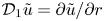 $\mathcal {D}_1\tilde {u}=\partial \tilde {u}/\partial r$.
Subscripts ‘ ${}_r$’ and ‘
 ${}_{rr}$’ denote the first and second derivatives with respect to the radial spatial direction for base state quantities. Derivatives of the base flow thermodynamic and transport properties with respect to the temperature and pressure introduced through (2.5) are indicated by the ‘
 $_{\bar {T}}$’ and ‘
 $_{\bar {p}}$’ subscripts. The non-dimensional number
 $\mathcal {H}=Ec\cdot c_p/\mathcal {R}$ introduced by Malik & Anderson (Reference Malik and Anderson1991) is used with
 $\mathcal {R}=287\ \textrm {J}\ \textrm {kg}^{-1}\ \textrm {K}^{-1}$ the gas constant for the undissociated
 $N_2\text {--}O_2$ mixture.
B.2. Mapping of the stability domain
Quantities involved in the stability problem are mapped from  $N$ points in the
 $r \in [0,r_{max}]$ domain onto the Chebyshev–Gauss–Lobatto points (
 $r_{CGL} \in [-1,1]$) defined by
 \begin{equation} r_{CGL} = \cos\left(\frac{k{\rm \pi}}{N}\right),\quad k=0,\ldots,N. \end{equation}
These points are further transformed using the tangent mapping from Bayliss & Turkel (Reference Bayliss and Turkel1992) yielding the stability points  $\eta$
 \begin{equation} \eta = \alpha_2+\frac{\tan(\lambda(r_{CGL} - r_0))}{\alpha_1}, \end{equation}
with
 \begin{gather} \kappa = \frac{\tan^{-1}(\alpha_1(1 + \alpha_2))}{\tan^{-1}(\alpha_1(1 - \alpha_2))}, \end{gather}
 \begin{gather}r_0 = \frac{\kappa - 1}{\kappa + 1}, \end{gather}
 \begin{gather}\lambda = \frac{\tan^{-1}(\alpha_1(1 + \alpha_2))}{1 - r_0}, \end{gather}
where the coefficients  $\alpha _1 \in \boldsymbol {R}^+$ and
 $\alpha _2 \in [0,1]$ control the points distribution.
B.3. Boundary conditions for the perturbation quantities
Centreline boundary conditions for the perturbations are derived from the boundedness and smoothness conditions introduced by Khorrami, Malik & Ash (Reference Khorrami, Malik and Ash1989). Depending on the value of the integral azimuthal wavenumber, these equations are completed by compatibility conditions obtained by linearly combining the linearized stability equations.
For  $m=0$, the smoothness conditions yield (B 10a), and the additional compatibility conditions are given (B 10b) and (B 10c).
 \begin{gather} \tilde{v} = \tilde{u} = 0 \end{gather}
 \begin{gather}\tilde{w}_r=\tilde{T}_r=0 \end{gather}
 \begin{gather}\textrm{i}\alpha\tilde{w} + 2\tilde{u}_r = ( \textrm{i}\omega - \textrm{i}\alpha\bar{W})\left(\frac{\bar{F}\tilde{p}}{\bar{P}} - \frac{\bar{G}\tilde{T}}{\bar{T}} \right). \end{gather}
For  $|m|=1$, the smoothness conditions yield (B 11a) and the compatibility conditions are given (B 11b) and (B 11c).
 \begin{gather} \tilde{w}=\tilde{T}=\tilde{p}=0, \end{gather}
 \begin{gather}\textrm{i} m \tilde{v}+\tilde{u}=0, \end{gather}
 \begin{gather}\tilde{u}_r(3\bar{\mu}+2\bar{\lambda})+\textrm{i}m\bar{\lambda}\tilde{v}_r=0, \end{gather}
where  $\lambda$ is the second viscosity coefficient given by Stokes’ hypothesis:
 $\lambda =-\frac {2}{3}\mu$. For
 $|m|>1$, the conditions of Khorrami et al. (Reference Khorrami, Malik and Ash1989) are sufficient and yield homogeneous Dirichlet for each perturbation variables.
Note that for the CPG assumption, the centreline boundary conditions are identical to the one presented here for LTE, with the exception that  $\bar {F} = \bar {G} = 1$ in (B 10c).