Building a New Measure and Theory of Cabinet Coalescence

In Latin America, 67 percent of presidents without an electoral majority have built government coalitions by means of cabinet management (Figueiredo et al. Reference Figueiredo, Salles and Vieira2010).^{Footnote 2} When cohesiveness can be observed within the created group, support for the president’s agenda will be effective (Figueiredo and Limongi Reference Figueiredo and Limongi1999; Zucco Reference Zucco2013).

Studies of Latin American multiparty presidential systems point to coalition management (cabinet positions, pork, and policy concessions) as the prime tool for the effective working of multiparty presidential regimes (Raile et al. Reference Raile, Pereira and Power2011) and an efficient cost of governing (Pereira et al. Reference Pereira, Bertholini and Raile2016). They also claim that allocations of cabinet positions and pork to coalition allies are imperfect substitutes for presidential legislative success. Arretche and Rodden (Reference Arretche and Rodden2004) argue that government coalitions built by means of cabinet appointments induce ministers to act as bridges between the federal executive and the congress, consequently being a cheaper coalition management tool than direct case-by-case negotiations with legislators. Martínez-Gallardo (Reference Martinez-Gallardo2011a, b) proposes that presidents choose cabinet appointments to build their coalitions only when they find their other available coalition management tools too costly. She also points out that cabinet stability is negatively related to the president’s constitutional powers, as well as to minority governments. Regarding the cabinet’s levels of partisanship, Amorim Neto and Strøm (Reference Amorim Neto and Strøm2006) and Amorim Neto and Samuels (Reference Amorim Neto and Samuels2010) indicate that the proportion of technocrat (or expert) ministers with no party affiliation inside the cabinet is generally negatively related to congressional fragmentation.

The 1988 Brazilian Constitution establishes a presidential system with open-list and proportional representation for electing legislators, which provides incentives for multiparty systems. In order to avoid potential governability problems of minority governments, which used to be very common in the previous period of democracy (1946–64), the Constituent Assembly also delegated the bulk of powers to the president. This combination has provided incentives for multiparty presidentialism and coalition government under the president’s coordination. In this institutional environment, therefore, it is mandatory for presidents to build postelectoral coalitions in order to achieve reasonable levels of governability and legislative success, consequently avoiding high levels of political distress (Negretto Reference Negretto2006).

Cabinets are analyzed according to various criteria, one of which considers the level of proportionality. The best-known measure of cabinet proportionality, namely coalescence, rests on the ratio between the number of ministries offered to a particular coalition partner and the number of congressional seats this same party holds in the ruling coalition. This measure allows us to observe whether a party with few seats receives a higher or lower number of ministries to control than its political weight in Congress; that is, if the coalition partner has been over- or underrewarded by the president. Empirically, it has been demonstrated that cabinet proportionality and party discipline favoring the president’s agenda have a positive relationship (Amorim Neto Reference Amorim Neto2000, Reference Amorim Neto, Morgenstern and Nacif2002, Reference Amorim Neto2006; Amorim Neto and Tafner Reference Amorim Neto and Tafner2002; Amorim Neto et al. Reference Amorim Neto, Cox and McCubbins2003).

Even while acknowledging that ministries differ from one another, however, the pertinent literature has not yet demonstrated this fact. Moreover, previous studies of the degree of coalescence have not considered ministries’ differences while computing cabinet proportionality. This has led to results obtained from the standard coalescence measure to be inappropriate to assess the true power held by coalition parties in presidential cabinets.

Instead of assuming that all ministries hold the same weights in the calculations of coalescence, we propose, on the contrary, both theoretically and empirically, that ministries differ when each one has a different level of political attractiveness. While some ministries are more attractive to one kind of party and coalition partner, others are preferred by other kinds of parties and politicians. Consequently, each ministry should be assigned a different mathematical weight when cabinet coalescence is computed.

We propose that differences in the political attractiveness of ministries rely on their different levels of budgetary capacities, regulatory capacities, networking capacities, and patronage capacities, as well as on politicians’ different preferences regarding those capacities.

By proposing that ministries differ from one another, with some being more desirable than others, we build a refined coalescence measure that produces different results from the standard coalescence degree obtained under the assumption that all ministries are equal.

Measuring Coalescence

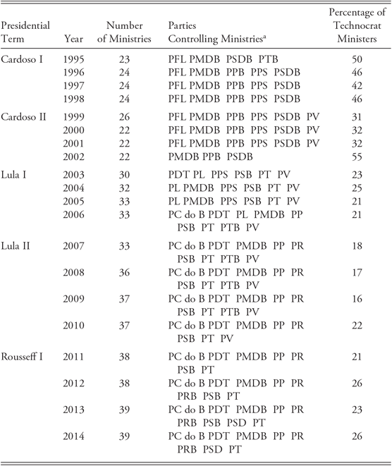
Our analysis comprises five presidential terms of three Brazilian presidents: Fernando Henrique Cardoso (1995–2002), Luis Inácio Lula da Silva (2003–10), and Dilma Rousseff (2011–14).^{Footnote 3} From 1995 to 2014, Brazil had 46 different ministries, some of which no longer exist or have changed their names.^{Footnote 4} Table 1 identifies cabinet composition year by year.^{Footnote 5}

Table 1.

Cabinet Composition by Year, 1995–2014

Source: Portal da Legislação, Library of the Presidency of Brazil, ministers’ and ministries’ websites.

^a Data refer to the party that held control for the most number of days in the referenced year. See list of acronyms.

The standard coalescence degree of a cabinet cab during year y is defined by equation 1 below (Amorim Neto Reference Amorim Neto2000, Reference Amorim Neto2006).

(1) $$ Standard\;Coalescence_{cab}^y = 1 - 1/2\sum\nolimits_{{\rm{\theta }} = 1}^n {\left( {|S_\theta ^y - M_\theta ^y|} \right)} $$

Where

$S_{\rm{\theta }}^y$ is the number of seats held by the coalition party θ in relation to the total number of Chamber of Deputies seats the whole government coalition held during year y.

$M_{\rm{\theta }}^y$ is the number of ministries controlled by the coalition party θ in relation to the total number of ministries in the cabinet during year y.

Maximum coalescence, or proportionality, is reached when Standard Coalescence = l.

As noted, our main concern regarding this standard coalescence measure relies on its assumption that all ministries composing $M_{\rm{\theta }}^y$ are equal and have the same

level of political attractiveness, holding the same weight in equation 1. To show how problematic such an assumption can be, consider, for example, what it would mean for a coalition party to choose between controlling the Ministry of Fishing and Aquaculture or the Ministry of Finance.^{Footnote 6}

Because our main purpose is to refine that standard coalescence degree by measuring ministries’ political attractiveness, we suggest a substitute for $M_{\rm{\theta }}^y$ . To do so, we first define the score of political attractiveness for the αth ministry during year y as in equation 2 below:

(2) $$ PA_\alpha ^y = \mathop \sum \nolimits_{i + 1}^7 v_i^yw_i^y $$

Where

$PA_{\rm{\alpha }}^y$ is the score of political attractiveness of the α th ministry during year y; $v_i^y$ is the value of the ith variable (or capacity) of political attractiveness during year y;

$w_i^y$ is the weight of the ith variable (or capacity) of political attractiveness during year y.

Once we find each ministry’s score of political attractiveness PA, we are able to compute the real share of the θth coalition party within the whole cabinet cab during year y.

(3) $$ RS_{\rm{\theta }}^y = {{\mathop \sum \nolimits_{{\rm{\alpha }} = 1}^n PA_{{{\rm{\alpha }}_{\rm{\theta }}}}^y} \over {\mathop \sum \nolimits_{all = 1}^n PA_{al{l_{cab}}}^y}} $$

Where

$RS_{\rm{\theta }}^y$ is the real share of the cabinet of the θth coalition party during year y, considering our proposition that ministries have different levels of political attractiveness;

$\sum\nolimits_{{\rm{\alpha }} = 1}^n P A_{{{\rm{\alpha }}_{\rm{\theta }}}}^y$ is the sum of the political attractiveness of every ministry α controlled by the θth coalition party during year y; and

$\sum\nolimits_{all = 1}^n P A_{al{l_{cab}}}^y$ is the sum of the political attractiveness of ministries that compose the presidential cabinet during year y.

Based on that, the refined coalescence degree of a cabinet during year y, measured according to our proposition that ministries hold different levels of political attractiveness, will be defined by substituting $M_{\rm{\theta }}^y$ by $RS_{\rm{\theta }}^y$ in equation 1:

(4) $$ Refined\;Coalescence_{cab}^y = 1 - 1/2\mathop \sum \nolimits_{{\rm{\theta }} = 1}^n \left( {|S_{\rm{\theta }}^y - RS_{\rm{\theta }}^y|} \right) $$

And substituting (3) in (4), we finally have:

(5) $$ Refined\;Coalescence_{cab}^y = 1 - 1/2\mathop \sum \nolimits_{{\rm{\theta }} = 1}^n \left( {|S_{\rm{\theta }}^y - \left( {{{\mathop \sum \nolimits_{{\rm{\alpha }} = 1}^n PA_{{{\rm{\alpha }}_{\rm{\theta }}}}^y} \over {\mathop \sum \nolimits_{all = 1}^n PA_{al{l_{cab}}}^y}}} \right)|} \right) $$

Patronage Capacity

There are several studies about patronage and its relation to politics in Latin America. Barberia and Praça (Reference Barberia and Praça2014) extensively discuss the process of choosing political appointees to government agencies in Brazil. Schneider (Reference Schneider1993) investigates the level of bureaucratic insulation and independence of Brazilian civil servants. He argues that civil servants tend to be less independent from politicians in Brazil. Lopez and Praça (Reference Lopez and Praça2015) find few changes occurring in Brazil toward more professionalized management practices in public agencies.

We identified two channels of influence over job nominations a coalition party might have. The first, Career Civil Servants, is the total number of regular employees of a ministry. These people are hired by a competitive examination system and are protected by strict rules about job tenure. Thus they are not directly appointed by politicians. Nevertheless, when a coalition partner runs a cabinet, it may be in a party’s interest to take actions that are favorable to all the employees, expecting to receive political benefits. As an example, let us consider the case of the Ministry of Education: by dealing with thousands of teachers, a specific policy implemented by the minister that favors teachers’ wages or work routines may generate political returns to the minister or the minister’s party in the next election. In addition, based on Schneider’s Reference Schneider1993 conclusions about the low level of bureaucratic insulation in Brazil, we infer that civil servants’ professional lives might be directly influenced by the decisions ministers make.

The second variable related to patronage capacity, Appointed Civil Servants, refers to the number of political appointees of a ministry. This is more related to a patronage strategy itself and is determined by the number of employees who occupy senior management and advisory positions (Direção e Assessoramento Superior, DAS) in a ministry. According to Barberia and Praça (Reference Barberia and Praça2014), DAS positions are freely appointed according to political criteria only.^{Footnote 9}

The data source for both variables for patronage capacities is the Ministry of Economic Planning, Budget, and Management.

After introducing all the variables of political attractiveness, the score of political attractiveness of the αth ministry during year y will now be:

(6) $$\displaylines{ PA_\alpha ^y = (Budget_\alpha ^y \times w_{budget}^y) + \cr (Unrestricted\;Expenses_\alpha ^y \times w_{Unrestricted\;Expenses}^y) + \cr (Regulatory_\alpha ^y \times w_{Regulatory}^y) + \cr (Networking_\alpha ^y \times w_{Networking}^y) + \cr (Career\;Civil\;Servants_\alpha ^y \times w_{Career\;Civil\;Servants}^y) + \cr (Appointed\;Civil\;Servants_\alpha ^y \times w_{Appointed\;Civil\;Servants}^y) \cr} $$

Where

$PA_{\rm{\alpha }}^y$ is the score of political attractiveness of the αth ministry during year y;

$Budget_{\rm{\alpha }}^y$ is the budget of the αth ministry in relation to the budget of all ministries during year y; $Unrestricted\;Expenses_{\rm{\alpha }}^y$ is the unrestricted expenses of the αth ministry in relation to the unrestricted expenses of all ministries during year y;

$Regulatory_{\rm{\alpha }}^y$ is a dummy variable equal to 1 if the α th ministry had under its domain at least one regulatory agency during year y and 0 otherwise;

$Networking_{\rm{\alpha }}^y$ is the number of agencies, companies, and other entities attached to the α th ministry in relation to the number of these same entities of all ministries during year y;

$Career\;Civil\;Servants_{\rm{\alpha }}^y$ is the number of regular employees of the αth ministry in relation to the number of employees of all ministries during year y;

$Appointed\;Civil\;Servants_{\rm{\alpha }}^y$ is the number of political appointees of the αth ministry in relation to the total number of all ministries during year y; and

w is the weight of each variable (or capacity) of political attractiveness during year y.

Weighting the Political Attractiveness Variables

We must now define the w_i values in equations 2 and 6. We propose that any definition based solely on our presumptions might be misleading. In order to solve such an issue, we carried out an elite survey among Brazilian legislators, who, in fact, often have the opportunity to choose a ministry to be controlled by their party. They were asked to classify the most important features that a ministry should have and to differentiate between the most and the least attractive ministries in Brazil.^{Footnote 10}

The elite survey was conducted from June 9 to July 17, 2015. We sent 129 questionnaires to all legislators who were members of the Chamber of Deputies leadership, chairpersons or first vice chairpersons of Chamber standing committees, leaders or first vice leaders of party delegations (or caucuses), or lawmakers who had served at least five terms in a row.^{Footnote 11} They were invited to answer electronically 17 questions classifying variables from not important to extremely important, as well as to rank ministries and give their opinion about the way Brazilian presidents manage their coalitions. (For further details about the survey, please see the online appendix.)

We made this choice of more senior and prominent legislators because the opinions of new legislators might not depict the proper weights that one could expect for the variables, since novice lawmakers do not have the same levels of congressional and political experience as senior legislators. Likewise, legislators’ views truly reflect what really matters when someone discusses ministries, since these politicians are usually responsible for appointing their party fellows to occupy such positions.^{Footnote 12} Answers that came from the legislators themselves, their chiefs of staff, or their senior legislative assistants were accepted, as we consider that high-ranking staff members would not go against their bosses’ opinion on a wide range of subjects, including ours. Out of the 129 questionnaires sent, we received 62 validly answered, resulting in a 48 percent response rate.

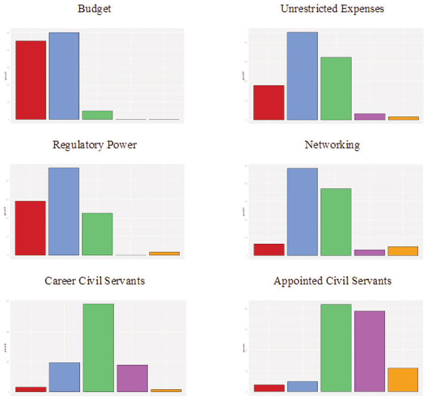
Focusing on the variables of political attractiveness discussed above, figure 1 presents legislators’ opinions about ministries’ levels of attractiveness. The elite survey reveals that budgetary capacities are highly regarded by the respondents, with the total budget being more attractive to them than the unrestricted expenses. Another very important capacity is regulatory capacity. The networking capacity came next. Last came the patronage capacities.

Figure 1.

Legislator Scale: Political Attractiveness Variables

Notes: Red bars = “Extremely important”; Blue bars = “Very important”; Green bars = “Moderately important”; Purple bars = “Relatively unimportant”; Orange bars = “Not important.” Answered questions: 62Source: Authors, based on legislators’ responses to the survey

Given our intention to quantify the item attractiveness ratings obtained from the answers presented in figure 1, we needed to find a way to translate the respondents’ opinions into quantitative weights. Because the literature offers no consensus about the best method to use when translating qualitative opinions into quantitative data, we considered the balanced statistic approach as appropriate for this purpose. This is expressed as follows.^{Footnote 13}

(7) $$ Balanced\;Statisti{c_i} = \mathop \sum \nolimits_{j = 1}^2 HighlyAttractiv{e_j} - \mathop \sum \nolimits_{k = 1}^2 slightlyAttractiv{e_k} $$

Where

Balanced Statistic_i, is the well-adjusted statistic for the answers concerning the ith variable (or capacity) of political attractiveness;

$\sum\nolimits_{j = 1}^2 Highly\;Attractiv{e_j}$ , is the sum of the j answers evaluating the variable (or capacity) of political attractiveness as highly attractive (“extremely important” and “very important” answers in the elite survey);

$\sum\nolimits_{k = 1}^2 Slightly\;Attractiv{e_k}$ is the sum of the k answers evaluating the variable (or capacity) of political attractiveness as slightly attractive (“relatively unimportant” and “not important” in the elite survey).

Because there could be a situation in which $\sum\nolimits_{j = 1}^2 Highly\;Attractiv{e_j}$ , is smaller than $\sum\nolimits_{k = 1}^2 Slightly\;Attractiv{e_k}$ resulting in Balanced Statistic_i < 0, we performed a logarithmic transformation, as specified in equation 8, to make all the weights positive. Since we previously proposed that all variables of political attractiveness we tested must be positive for all political parties, differing from one another only regarding the magnitude of this positive level of attractiveness, it would be senseless to suppose a condition in which Balanced Statistic_i < 0, implying that some of the variables of political attractiveness would be liabilities instead of assets. Indeed, the questions identified in figure 1 have positive answers, differing only between those expressing strong attractiveness of the variable and those indicating the variable is not so attractive but never undesirable. The previous explanation leads us to

(8) $$ Transformed\;Balanced\;Statisti{c_j} = {\rm{In}}(Balanced\;Statisti{c_i} + \Phi ) $$

Where

Transformed Balanced Statistic_i is the transformed balanced statistic of the ith variable (or capacity) of political attractiveness;

Φ is the same constant added to the Balanced Statistic_i, of all variables (or capacities) of political attractiveness. It is defined such that min(Balanced Statistic_i) + Φ = 1.01.^{Footnote 14}

Based on this formula, each variable (or capacity) of political attractiveness weight (w_i) is obtained according to equation 9.^{Footnote 15}

(9) $$ {w_i} = {{Transformed\;Balanced\;Statisti{c_i}} \over {\sum\nolimits_{i = 1}^7 T ransformed\;Balanced\;Statisti{c_i}}} $$

After performing the steps defined by equations 7, 8, and 9, the weights are budget 0.2236, unrestricted expenses 0.2110, regulation 0.2178, networking 0.1719, career civil servants 0.1752, and appointed civil servants 0.0005.^{Footnote 16} From these findings and based on equations 2 and 6, we have the political attractiveness of the αth ministry during year y measured by

(10) $$\displaylines{ PA_\alpha ^y = (Budget_\alpha ^y \times 0.2236) + \cr (Unrestricted\;Expenses_\alpha ^y \times 0.2110) + \cr ({\mathop{\rm Re}\nolimits} gulatory_\alpha ^y \times 0.2178) + \cr (Networking_\alpha ^y \times 0.1719) + \cr (Career\;Civil\;Servants_\alpha ^y \times 0.1752) + \cr (Appo{\mathop{\rm int}} ed\;Civil\;Servants_\alpha ^y \times 0.0005) \cr} $$

^{Footnote 17}

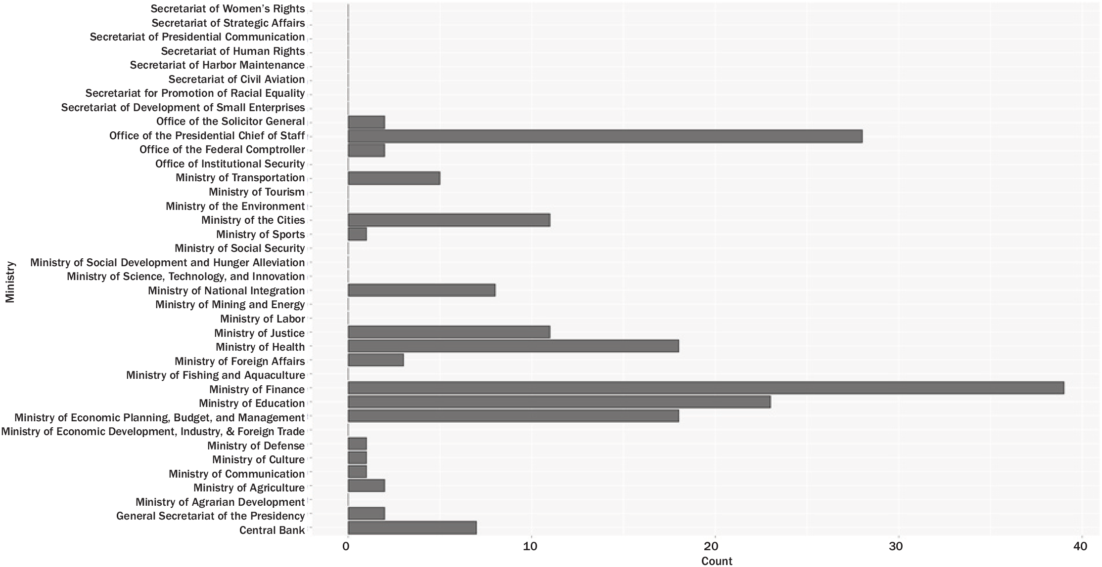
To identify the ministries’ political attractiveness, we also asked legislators in the survey to directly rank the most and least politically attractive ministries. As figure 2 shows, legislators rated the five most attractive ministries as the Ministry of Finance, the Office of the Presidential Chief of Staff, the Ministry of Education, the Ministry of Health, and the Ministry of Economic Planning, Budget, and Management.

Figure 2.

Most Politically Attractive Ministries in Brazil, According to Legislators

Answered questions: 61Source: Authors, based on legislator survey

Comparing Coalescence Measures and Their Effect on Legislative Support

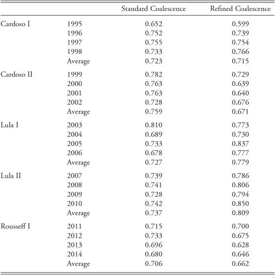
Table 2 presents the refined coalescence degree obtained from our proposal, which considers different levels of political attractiveness of ministries, obtained through equations 4 and 5. It also presents the standard coalescence degree built under the current assumption that ministries’ different levels of political attractiveness are not considered, which was obtained through equation 1.

Table 2.

Cabinet Coalescence Measures, 1995–2014

Note: Even though Central Bank characteristics are considered here, they were not considered for coalescence purposes, since the head is the only member of the cabinet who needs congressional approval. Refined coalescence was obtained through equations 4 and 5, based on our proposition that the different levels of ministries’ political attractiveness should be considered. Standard coalescence was obtained through equation 1, based on the proposition of the current literature that ministries’ different levels of political attractiveness do not need to be considered. Source: Authors

As the table shows, the differences between the two measures are quite significant in many years. The cabinets in 2000 and 2001 were approximately 16 percent less coalescent when one considers our measure instead of the standard one. In 2005, 2006, and 2010, the cabinets were approximately 14 percent more coalescent under our measure. In only three years (1996, 1997, and 2011) of the entire period analyzed were the differences between the two measures small. In several other years, the differences ranged from 7 to 9 percent, revealing that our refined coalescence measure does substantively differ from the standard one in absolute terms.

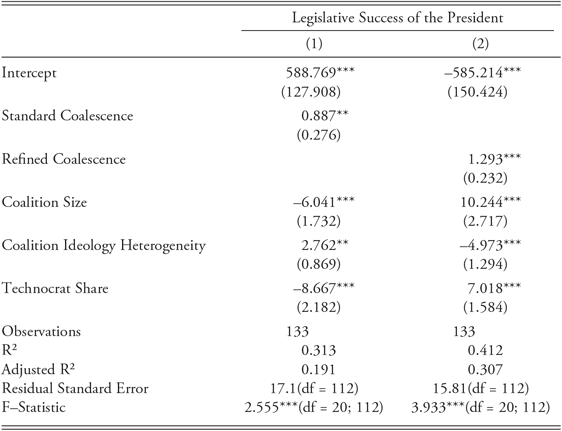
We performed two estimations with fixed effects panels in order to validate our measure of coalescence against the standard one. By comparing the R² and the Adjusted R2 scores of two different models that estimate the same phenomenon, we can assess which measure of coalescence is more accurate or has greater explanatory power (Kalt and Zupan Reference Kalt and Zupan1984; Kau and Rubin Reference Kau and Rubin1979).

The dependent variable is the legislative success of the president. Specifically, it is the percentage of support from a coalition party in favor of presidential bills. Standard Coalescence is the main explanatory variable in model 1, depicting the coalitional surplus under the standard approach; that is, the difference between the percentage of the cabinet each party has, considering the standard measure that all ministries are equal and the of Chamber seats in the coalition that the same party holds (the term $|S_{\rm{\theta }}^y - M_{\rm{\theta }}^y|$ in equation 1). On the other hand, Refined Coalescence is the main explanatory variable in model 2, reflecting the coalitional surplus of each party, considering our refined measure (the term $|S_{\rm{\theta }}^y - RS_{\rm{\theta }}^y|$ in equation 4).

In the specifications of legislative success, we decided not only to replicate Amorim Neto’s models (Reference Amorim Neto, Morgenstern and Nacif2002) but also to include other coalition management variables as controls: Coalition Size (the number of parties controlling at least one ministry), Coalition Ideological Heterogeneity (coefficients of variation—a ratio between standard deviation and mean—of the ideologies of all the parties that formed the coalition), and Technocrat Share, which controls for the percentage of nonpartisan ministers in the cabinet in each year.

Bertholini and Pereira (Reference Bertholini and Pereira2017) demonstrate that large coalitions, with greater numbers of parties, tend to face higher coordination problems and therefore, greater difficulties in maintaining coalition discipline over time. They also show that coalitions with greater ideological diversity are also more difficult to coordinate and manage, so the president will face greater problems in Congress. Based on this evidence, we also expect that the greater the ideological heterogeneity of the governing coalition, the smaller the presidential support in Congress. In addition, we expect that the larger the share of nonpartisan ministers in the cabinet, the smaller the presidential support in Congress will be.

The results in table 3 show that the greater the coalescence between the cabinet portfolio received and the number of Chamber seats held by a coalition party, the higher the political support for the president in the period studied. In model 1, an increase of 1 percent in the cabinet coalescence was associated with an increase of 0.887 percent in presidential success, on average. In model 2, an increase of 1 percent in the cabinet coalescence was associated with an increase of 1.293 percent in support for the president in Congress, on average. Substantively speaking, by applying our specification of the refined measure of coalescence, the coefficient is larger than that obtained by applying the standard measure (1.293 against 0.887, respectively).

Table 3.

Legislative Success of the President (fixed effects), 1995–2014

*p < 0.1; **p < 0.05; ***p < 0.01

Another aspect to be highlighted is that the R2 and the adjusted R2 of model 2, the model using our refined measure of coalescence, were greater by approximately 10 percent than those obtained by the model with the standard measure (0.412 against 0.313 regarding R2 and 0.307 against 0.191 regarding adjusted R2, respectively). These results suggest that when we consider politicians’ substantive differences among ministries, the refined coalescence measure presents a better fit. The R2 and the adjusted R2 comparisons show that our refined coalescence measure has stronger explanatory power than the standard one. Therefore, the econometric exercises show how our new measure of coalescence improves the understanding of coalition governments in multiparty presidential regimes.