1 Introduction
In many turbulent flows such as boundary layers, jets and wakes, which are ubiquitous in atmospheric and engineering flows, several studies have highlighted the presence of sharply defined edges or interfacial layers. The nature of the interface between turbulent and non-turbulent fluids has been of particular interest over the last half-century. Early seminal work in the 1950s presented the first empirical evidence of this interfacial layer (Corrsin & Kistler Reference Corrsin and Kistler1955), which is now commonly referred to as the turbulent/non-turbulent interface, or TNTI. Over the last few decades, investigators have examined these interfacial layers using new experimental techniques and numerical databases (summarised recently by da Silva et al. (Reference da Silva, Hunt, Eames and Westerweel2014)), highlighting their importance to the overall dynamics of turbulent flows. For example, the presence of a sharp change in velocity at the TNTI, postulated initially by Corrsin & Kistler (Reference Corrsin and Kistler1955) has been reported in boundary layers (Semin et al. Reference Semin, Golub, Elsinga and Westerweel2011; Chauhan et al. Reference Chauhan, Philip, de Silva, Hutchins and Marusic2014b ; Ishihara, Ogasawara & Hunt Reference Ishihara, Ogasawara and Hunt2015), jets (Westerweel et al. Reference Westerweel, Fukushima, Pedersen and Hunt2005), wakes (Bisset, Hunt & Rogers Reference Bisset, Hunt and Rogers2002) and shear free flows (Holzner Reference Holzner and Lüthi2011). A number of studies have also focused on examining the entrainment of non-turbulent fluid (Mathew & Basu Reference Mathew and Basu2002; Westerweel et al. Reference Westerweel, Fukushima, Pedersen and Hunt2009; Philip & Marusic Reference Philip and Marusic2012, and others), a phenomenon known to dictate numerous physical processes in nature such as the evolution of clouds, volcanic eruptions, to name a few.
Comparable interfacial layers similar to the TNTI (an external interface) have also been reported within the turbulent region of flows, which are broadly referred to as internal interfaces or shear layers. Their presence and importance in boundary layers are highlighted in a review article by Robinson (Reference Robinson1991). These findings are discussed by means of statistical tools such as space–time correlations from single point measurements (Blackwelder & Kovasznay Reference Blackwelder and Kovasznay1972) and linear stochastic estimations from spatial data (Christensen & Adrian Reference Christensen and Adrian2001; Hambleton, Hutchins & Marusic Reference Hambleton, Hutchins and Marusic2006). Recent work by Eisma et al. (Reference Eisma, Westerweel, Ooms and Elsinga2015) highlighted the presence of internal layers of strong shear within the turbulent region of a boundary layer. Following prior work, at the TNTI they reported that these layers which comprise of high shear have characteristically similar properties to those previously reported at the TNTI. Further, based on theoretical concepts they determined entrainment velocities at the interfaces which revealed that the interfaces move up away from the wall at comparable rates to the TNTI. Ishihara, Kaneda & Hunt (Reference Ishihara, Kaneda and Hunt2013) reported comparable interfacial layers in isotropic turbulence and suggested that they exhibit similar characteristics to the TNTI in boundary layers and wakes. Their work highlighted the significant dynamical processes occurring at these interfacial layers within the turbulent region, where a large proportion of vorticity is present.
Among the plethora of coherent structures reported in turbulent boundary layers, regions of uniform streamwise momentum (more commonly referred to as uniform moment zones, or UMZs), first reported by Meinhart & Adrian (Reference Meinhart and Adrian1995), have been shown to be strongly associated with interfacial layers. Specifically, these regions of uniform momentum are demarcated by thin interfacial layers/interfaces of strong shear, where a large proportion of the vorticity is clustered in turbulent boundary layers (Adrian, Meinhart & Tomkins Reference Adrian, Meinhart and Tomkins2000; Eisma et al.
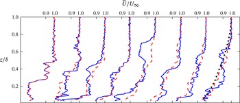
Reference Eisma, Westerweel, Ooms and Elsinga2015). Collectively, these findings highlight a zonal-like structure in turbulent boundary layers which is illustrated in figure 1, where the solid (blue) lines (–) show a set of instantaneous streamwise velocity (
 $\widetilde{U}$
) profiles in the wall-normal direction. The profiles are at a friction Reynolds number,
 $Re_{\unicode[STIX]{x1D70F}}=\unicode[STIX]{x1D6FF}U_{\unicode[STIX]{x1D70F}}/\unicode[STIX]{x1D708}\approx 8000$
, where
 $U_{\unicode[STIX]{x1D70F}}$
is the friction velocity,
 $\unicode[STIX]{x1D6FF}$
is the boundary layer thickness and
 $\unicode[STIX]{x1D708}$
is the kinematic viscosity. Each of these profiles reveal that the streamwise velocity in a boundary layer typically exhibits a step-like profile with sharp changes in momentum flanked by regions of nominally uniform momentum as a function of wall-normal height. On the other hand, the overlaid (red) dashed lines (– –) which correspond to a cumulative average of the instantaneous profiles (blue solid lines) from left to right exhibit an increasingly smooth profile ultimately converging to the temporally averaged mean flow statistics (shown by the black dots).
The high shear regions in turbulent boundary layers, where sharp changes in momentum occur, have been thought to signify large coherent motions in turbulent boundary layers, including: packets of hairpin heads (Head & Bandyopadhyay Reference Head and Bandyopadhyay1981; Adrian et al.
Reference Adrian, Meinhart and Tomkins2000, and others), vortex clusters (del Alamo et al.
Reference del Alamo, Jiménez, Zandonade and Moser2004) and vortical fissures (Priyadarshana et al.
Reference Priyadarshana, Klewicki, Treat and Foss2007). A similar zonal-like structural arrangement with concentrated regions of shear has also been reported for internal flows in channels and pipes (Kwon et al.
Reference Kwon, Philip, de Silva, Monty and Hutchins2014). More recently, utilising experimental datasets that span over a decade of Reynolds number (
 $Re$
), de Silva, Hutchins & Marusic (Reference de Silva, Hutchins and Marusic2016) reported a clear log–linear increase in the number of UMZs with increasing
 $Re$
. This work highlighted a hierarchical length scale distribution of coherent structures in a zonal-like arrangement, which in turn results in a step-like instantaneous profile for the streamwise momentum as a function of wall-normal height. In contrast, the temporally averaged streamwise momentum of a boundary layer exhibits a smooth profile (see figure 1), with no evidence of sharp changes in momentum. Gaining further insight on these differences and how the instantaneous dynamics manifests itself in the temporally averaged flow statistics will be explored in the present study.
Comparison between instantaneous velocity profiles
 $\widetilde{U}$
and an averaged velocity profiles in the wall-normal direction (
 $z$
) at
 $Re_{\unicode[STIX]{x1D70F}}\approx 8000$
. The solid blue lines correspond to eight independent instantaneous velocity profiles. Each (red) dashed line corresponds to a cumulative average of the instantaneous profiles from left to right (the rightmost (red) dashed line is an average of all the eight instantaneous profiles shown in this illustration). The black dotted line corresponds to the converged mean streamwise velocity profile from the same database.

Accordingly, we focus our attention to the edges that demarcate UMZs within the turbulent region of a turbulent boundary layer, which has not received significant attention to date, particularly at high Reynolds numbers. Specifically, understanding how the instantaneous step-like velocity distribution manifests in the temporally averaged flow statistics (as illustrated in figure 1) requires a thorough characterisation of the UMZ edges across a range of Reynolds numbers. The paper is organised as follows: § 2 provides a description of the experimental databases used, which is followed by an outline of the scheme employed to detect the presence of UMZs and their associated edges (§ 3). Section 4 examines properties at these UMZ edges such as their spatial arrangement, geometric properties, and determining the magnitude of the step-like change in momentum that occurs in the near vicinity. Section 5 examines the scaling of these parameters based on experimental evidence and theoretical reasoning. Finally, the relevant parameters are combined in § 6 towards constructing the temporarily averaged statistical behaviour of a turbulent boundary layer. As an aside, throughout our analysis comparisons are drawn between the edges of UMZs which demarcate two nominally turbulent regions (or internal interfaces), and the outermost UMZ edge which separates a non-turbulent region from a turbulent region (the TNTI).
In this paper, we use the coordinate system
 $x$
,
 $y$
and
 $z$
to refer to the streamwise, spanwise and wall-normal directions, respectively. Corresponding instantaneous streamwise, spanwise and wall-normal velocities are represented by
 $\widetilde{U}$
,
 $\widetilde{V}$
and
 $\widetilde{W}$
, respectively, with the corresponding velocity fluctuations given by lower case letters. Capitalisation and overbars indicate averaged quantities, and angle brackets correspond to conditionally averaged statistics. Superscript
 $+$
refers to normalisation by inner scales. For example, for length we use
 $l^{+}=lU_{\unicode[STIX]{x1D70F}}/\unicode[STIX]{x1D708}$
, and for velocity we use
 $U^{+}=\widetilde{U}/U_{\unicode[STIX]{x1D70F}}$
, where
 $U_{\unicode[STIX]{x1D70F}}$
is the friction velocity and
 $\unicode[STIX]{x1D708}$
is the kinematic viscosity of the fluid.
2 Experimental databases
The present study utilises particle image velocimetry databases with two-dimensional velocity fields in a streamwise/wall-normal plane. The databases span over a decade of friction Reynolds numbers from
 $Re_{\unicode[STIX]{x1D70F}}\approx 1200{-}14\,500$
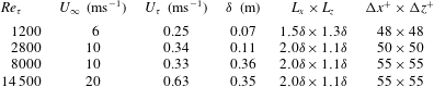
. Key experimental parameters of each database are summarised in table 1. The databases at
 $Re_{\unicode[STIX]{x1D70F}}\approx 2800,8000$
and 14 500 are acquired in the high Reynolds number boundary layer wind tunnel (HRNBLWT) at the University of Melbourne, using a unique experimental set-up with multiple cameras to obtain a large field of view of the order of the boundary layer thickness. We note the databases at
 $Re_{\unicode[STIX]{x1D70F}}\approx 8000$
and 14 500 have been examined previously (de Silva et al.
Reference de Silva, Gnanamanickam, Atkinson, Buchmann, Hutchins, Soria and Marusic2014; Chauhan et al.
Reference Chauhan, Philip, de Silva, Hutchins and Marusic2014b
, and others); however, due to the varying magnifications employed, the databases have been reprocessed to match the spatial resolution (or interrogation window size,
 $\unicode[STIX]{x0394}x^{+}\times \unicode[STIX]{x0394}z^{+}$
) in viscous units across the entire extent of the boundary layer. Further, the experimental databases at lower
 $Re$
have been spatially box filtered to match the spatial resolution of the higher
 $Re$
databases. It should be noted that for consistency, certain parameters are recomputed for the database from Hambleton et al. (Reference Hambleton, Hutchins and Marusic2006) by applying the composite velocity profile of Chauhan, Monkewitz & Nagib (Reference Chauhan, Monkewitz and Nagib2009). Further details on the datasets at
 $Re_{\unicode[STIX]{x1D70F}}\approx 1200,2800$
and 8000–14 500 can be found in Hambleton et al. (Reference Hambleton, Hutchins and Marusic2006), de Silva et al. (Reference de Silva, Chauhan, Atkinson, Buchmann, Hutchins, Soria and Marusic2015) and de Silva et al. (Reference de Silva, Squire, Hutchins and Marusic2012), respectively.
Experimental parameters of the four particle image velocimetry (PIV) databases employed.
 $L_{x}$
and
 $L_{z}$
correspond to the field of view of the streamwise wall-normal plane, and
 $\unicode[STIX]{x0394}x^{+}$
and
 $\unicode[STIX]{x0394}z^{+}$
correspond to the approximate interrogation window size in viscous units. All datasets are processed with 50 % vector overlap and each database has over 1000 independent PIV frames. Further details on the experiments at
 $Re_{\unicode[STIX]{x1D70F}}\approx 1200$
,
 $Re_{\unicode[STIX]{x1D70F}}\approx 2800$
and
 $Re_{\unicode[STIX]{x1D70F}}\approx 8000{-}14\,500$
can be found in Hambleton et al. (Reference Hambleton, Hutchins and Marusic2006), de Silva et al. (Reference de Silva, Chauhan, Atkinson, Buchmann, Hutchins, Soria and Marusic2015) and de Silva et al. (Reference de Silva, Squire, Hutchins and Marusic2012), respectively.

Although the present analysis utilises databases from multiple flow facilities, they are all acquired with large field of views on the order of the boundary layer thickness. Further, the spatial resolution in viscous units of the datasets is comparable (see table 1). For example, good spatial resolution in viscous units is hardest to achieve with the highest Reynolds number datasets, yet the interrogation window size is approximately six Kolmogorov length scales in the outer region. Further details on the accuracy of the data and the influence of spatial resolution can be found in de Silva et al. (Reference de Silva, Gnanamanickam, Atkinson, Buchmann, Hutchins, Soria and Marusic2014).
3 Detection and characteristics
In order to examine the high shear regions which demarcate uniform momentum zones, we start by examining the probability density functions (p.d.f.s) of the streamwise velocity component (Adrian et al.
Reference Adrian, Meinhart and Tomkins2000; Kwon et al.
Reference Kwon, Philip, de Silva, Monty and Hutchins2014; de Silva et al.
Reference de Silva, Hutchins and Marusic2016). This approach was originally introduced by Adrian and co-workers to detect the presence of UMZs by locating local maxima on the p.d.f. of
 $\widetilde{U}$
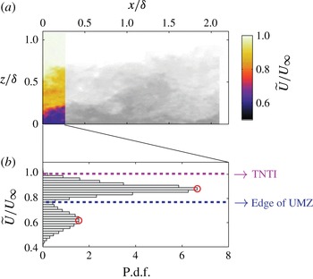
. Here we extend this technique to estimate the spatial location of the edges that demarcate UMZs. An illustration of the technique is shown in figure 2. Figure 2(a) shows a sample velocity field at
 $Re_{\unicode[STIX]{x1D70F}}\approx 8000$
(grey contours), where the colour contours indicate the included region used to construct the p.d.f. of streamwise velocity shown in figure 2(b). We note the streamwise extent of the included region (
 ${\mathcal{L}}_{x}$
) is chosen to be fixed at 2000 viscous units for the present study. Further, the non-turbulent region where
 $\widetilde{U}\approx U_{\infty }$
is not included in the p.d.f. by omitting all velocity vectors beyond the turbulent/non-turbulent interface. A detailed discussion on
 ${\mathcal{L}}_{x}$
and other criteria for detecting UMZs is discussed in de Silva et al. (Reference de Silva, Hutchins and Marusic2016) and is not reproduced here.
Illustration of detection criteria for edges of UMZs applied to an instantaneous velocity field at
 $Re_{\unicode[STIX]{x1D70F}}=8000$
. (a) Shows iso-contours of streamwise velocity (
 $\widetilde{U}$
) of the included region of a single PIV frame (colour), and omitted region in grey scale. (b) Shows the histogram of
 $\widetilde{U}/U_{\infty }$
constructed using the included region indicated in (a); (○) symbols indicate the detected modal velocities. The non-turbulent region is not included in constructing the p.d.f. shown in (b). Horizontal dashed lines represent streamwise velocity of the detected UMZ edges and the TNTI.

The peaks of the p.d.f. shown in figure 2(b) correspond to possible modal velocities,
 $\widetilde{U}_{m}$
, indicated by ○ symbols. The example shows two clear peaks in the p.d.f. (modal velocities) whose corresponding UMZs are also identifiable by visually inspecting figure 2(a). The magnitude of streamwise velocity at the edge of each detected UMZ typically resides in the near vicinity of the local minima on the p.d.f. of
 $\widetilde{U}$
, which is approximated by the mid-point between modal velocities of neighbouring UMZs in the present study. Figure 2(b) shows one such detected edge (or internal interface) at
 $\widetilde{U}/U_{\infty }\approx 0.8$
. The turbulent/non-turbulent interface is also included independently in this study and is considered as the outer edge of the UMZ furthest away from the wall. Unlike the internal interfaces within the turbulent region, a number of techniques have been employed in the past to detect the TNTI. These include methods based on thresholds of vorticity (Bisset et al.
Reference Bisset, Hunt and Rogers2002; Mathew & Basu Reference Mathew and Basu2002; Jiménez et al.
Reference Jiménez, Hoyas, Simens and Mizuno2010) and kinetic energy (de Silva et al.
Reference de Silva, Philip, Chauhan, Meneveau and Marusic2013; Chauhan et al.
Reference Chauhan, Philip, de Silva, Hutchins and Marusic2014b
). It is also known that velocity magnitudes differ between the turbulent and non-turbulent regions (Townsend Reference Townsend1976), therefore the mean velocity (Anand, Boersma & Agrawal Reference Anand, Boersma and Agrawal2009) and velocity fluctuations (Heskestad Reference Heskestad1965) have also been used to detect the TNTI. Of this range of techniques, not all are suited for every study and measurement technique. In the present case, since the spatial location of the internal interfaces is determined using a streamwise velocity magnitude (see figure 2), for consistency, we estimate the location of theTNTIusing aconstant streamwise velocitymagnitudeof
 $97\,\%U_{\infty }$
. With this approach, any influence of differing detection criteria used for the TNTI and internal interfaces is minimised for the comparisons to be presented in the subsequent analysis.
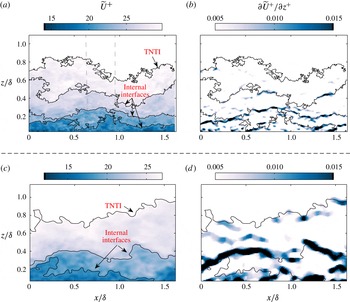
A sample instantaneous velocity field with all the detected edges of UMZs (inclusive of the TNTI) shown as black contour lines at
 $Re_{\unicode[STIX]{x1D70F}}\approx 8000$
, (a) overlaid on colour contours of streamwise velocity (
 $\widetilde{U}$
) from a single PIV frame, and (b) overlaid on
 $\unicode[STIX]{x2202}\widetilde{U}/\unicode[STIX]{x2202}z$
. (c,d) show (a,b) reproduced at a lower Reynolds number of
 $Re_{\unicode[STIX]{x1D70F}}\approx 2800$
.

A visual example of the described detection technique, applied to an instantaneous velocity field from a PIV dataset at
 $Re_{\unicode[STIX]{x1D70F}}\approx 8000$
, is shown in figure 3(a). The black contour lines within the turbulent region represent UMZ edges (or internal interfaces), whereas the topmost black contour line encapsulating the turbulent region of the flow represents the TNTI. We note that for this example the streamwise velocity magnitude of these contour lines for the internal interfaces is detected in the central 2000 viscous units indicated by the vertical dashed lines, thereafter the same contours are extended across the entire extent of the FOV. Although only extended for illustrative purposes, for the presented examples (cf. figure 3) only a subtle difference in modal velocity magnitude occurs at the detected UMZ edges across the entire FOV (
 ${<}5\,\%$
). Therefore, the presented UMZ edges are representative of the UMZ edges used in the subsequent analysis, where we compute results over a streamwise extent of 2000 viscous units. Additionally, although both the TNTI and internal interfaces are three-dimensional, here we are limited to planar two-dimensional vector fields hence the interface is detected as a line on the streamwise/wall-normal plane. Qualitatively, it is evident that at the detected edges of UMZs a sharp change in streamwise momentum is present. As a consequence, a large proportion of the shear in a turbulent boundary layer appears to reside at the detected UMZ edges. Further, we anticipate that the characteristic properties of these interfaces will be comparable and will complement recent work examining internal layers of high shear (Eisma et al.
Reference Eisma, Westerweel, Ooms and Elsinga2015).
We note the detected UMZ edges (inclusive of the TNTI) occasionally fold back on themselves, i.e. they are non-monotonic in the streamwise direction. Furthermore, small ‘pockets’ are commonly observed. These pockets are consistent with slicing through packet-like structures (see Adrian et al.
Reference Adrian, Meinhart and Tomkins2000) and remind us that we are examining a planar slice (
 $xz$
plane) of a convoluted three-dimensional surface (UMZ edges). However, for the present analysis, we will ignore these small pockets and primarily focus on examining the interface that extends from the left edge to the right edge of the vector field, unless otherwise stated.
The corresponding instantaneous wall-normal gradient of the streamwise velocity,
 $\unicode[STIX]{x2202}\widetilde{U}/\unicode[STIX]{x2202}z$
is shown in figure 3(b), which qualitatively reveals that a large proportion of high shear regions (to be quantified later) are present in the near vicinity of the interfaces that demarcate UMZs. Furthermore, they occur in concentrated patches along the edge. Previously, Adrian et al. (Reference Adrian, Meinhart and Tomkins2000) and others postulated that these regions of high
 $\unicode[STIX]{x2202}\widetilde{U}/\unicode[STIX]{x2202}z$
mark the possible presence of packet-like structures, where a significant proportion of the spanwise vorticity is concentrated. Therefore, in the present work as we consider these interfaces as lines, in doing so we average the properties of these patches of vorticity.
In order to illustrate the influence of
 $Re$
on the zonal-like structural organisation reported, figure 3(c,d) reproduces an instantaneous velocity field and its corresponding shear,
 $\unicode[STIX]{x2202}\widetilde{U}/\unicode[STIX]{x2202}z$
at a lower Reynolds number of
 $Re_{\unicode[STIX]{x1D70F}}\approx 2800$
. The results exhibit similar behaviour to the higher
 $Re$
databases (figure 3
a,b), however the zonal-like arrangement appears to be more prevalent at higher
 $Re$
. Specifically, the high
 $\unicode[STIX]{x2202}\widetilde{U}/\unicode[STIX]{x2202}z$
patches residing at the UMZ edges appear thinner, consequently the UMZ themselves occupy a larger fraction of the total boundary layer thickness at higher
 $Re$
. These qualitative observations will be revisited and quantified in § 5.
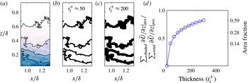
Illustration of inhomogeneity in high shear regions of a turbulent boundary layer. (a) Central region of the instantaneous velocity field shown in figure 3 reproduced. (b,c) A binary representation of (a), where the dark shaded regions correspond to UMZ edges with a thickness of (b)
 $t_{i}^{+}\approx 50$
and (c) 200 viscous units, respectively. (d) Fraction of the total positive shear in the turbulent boundary layer,
 $\sum _{total}\unicode[STIX]{x2202}\widetilde{U}/\unicode[STIX]{x2202}z|_{pos}$
, present within the shaded area representing UMZ edges
 $\sum _{shaded}\unicode[STIX]{x2202}\widetilde{U}/\unicode[STIX]{x2202}z|_{pos}$
as function of thickness,
 $t_{i}$
. Results are presented for the
 $Re_{\unicode[STIX]{x1D70F}}\approx 8000$
database and the right-hand ordinate represents the area fraction covered by the shaded region of the turbulent boundary layer.

To further explore the persistent presence of UMZs separated by sharp momentum changes in turbulent boundary layers, we examine the inhomogeneity of the shear,
 $\unicode[STIX]{x2202}\widetilde{U}/\unicode[STIX]{x2202}z$
. The process is illustrated in figure 4 using the central region of the same instantaneous velocity field presented earlier in figure 3. To separate the turbulent region into UMZs we associate a thickness,
 $t_{i}$
, to their edges, which is illustrated in figure 4(b,c). Specifically, the dark shaded regions in figure 4(b,c) correspond to
 $t_{i}^{+}\approx 50$
and 200 viscous units, respectively, where we anticipate a large proportion of the shear to be present. To quantify this, we compute the total summed positive shear present within the UMZ’s edges of thickness
 $t_{i}$
(i.e. within the shaded regions in figure 4
b,c),
 $\sum _{shaded}\unicode[STIX]{x2202}\widetilde{U}/\unicode[STIX]{x2202}z|_{pos}$
, and normalise this by the total positive shear within the turbulent region of the boundary layer,
 $\sum _{total}\unicode[STIX]{x2202}\widetilde{U}/\unicode[STIX]{x2202}z|_{pos}$
. We note the summations are equivalent to surface integrals, however, here we work on a discrete vector grid. The results are shown in figure 4(d) and are presented as a function of thickness,
 $t_{i}$
revealing that a substantial proportion of the total
 $\unicode[STIX]{x2202}\widetilde{U}/\unicode[STIX]{x2202}z$
resides at the detected UMZ edges. Further, due to the analogous behaviour between the shear and spanwise vorticity a large proportion of both quantities resides in the near vicinity of UMZ edges (see also Adrian et al.
Reference Adrian, Meinhart and Tomkins2000; Eisma et al.
Reference Eisma, Westerweel, Ooms and Elsinga2015). In fact, for example at
 $Re_{\unicode[STIX]{x1D70F}}\approx 8000$
over 50 % of the total positive shear is present within
 $100$
viscous units from these edges, which corresponds to an area fraction of approximately 15 % of the turbulent region in a boundary layer. Consequently, we observe sharp changes in momentum at these UMZ edges, and our results confirm the sparsity of shear within the UMZs themselves, which accounts for a significantly larger area fraction. We note, similar concentration levels of
 $\sum _{shaded}\unicode[STIX]{x2202}\widetilde{U}/\unicode[STIX]{x2202}z|_{pos}$
are also present across the other Reynolds numbers examined here. In § 4.3 we attempt to estimate the thickness of these UMZs, which leads to an investigation of the Reynolds number scaling of these interfaces in § 5.
4 Analysis
4.1 Distribution of UMZ edges in turbulent boundary layers
To examine the geometric properties of the detected UMZ edges as a function of wall-normal height, we first require a quantitative measure of its wall-normal location. To this end, since each UMZ edge has a spatially varying wall-normal location, we employ the streamwise momentum deficit defined as
 $$\begin{eqnarray}\displaystyle \widetilde{U}_{mom}^{+}=(U_{\infty }-\widetilde{U}_{i})/U_{\unicode[STIX]{x1D70F}}, & & \displaystyle\end{eqnarray}$$
as a surrogate for wall-normal position. Here,
 $\widetilde{U}_{i}$
corresponds to the streamwise velocity and is constant along each interface, therefore,
 $\widetilde{U}_{mom}^{+}$
is also constant along each detected interface. To illustrate that
 $\widetilde{U}_{mom}^{+}$
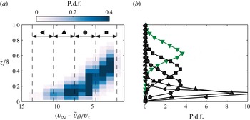
is a suitable candidate as a surrogate for wall-normal position, figure 5(a) shows a joint p.d.f. between
 $(U_{\infty }-\widetilde{U}_{i})/U_{\unicode[STIX]{x1D70F}}$
and
 $z$
, computed at each grid point along all detected UMZ edges. The results exhibit a clear reduction in wall-normal location with increasing momentum deficit, providing quantitative evidence that
 $\widetilde{U}_{mom}^{+}$
can be directly related to the wall-normal location. Therefore, for the subsequent analysis, we separate all detected edges of UMZs based on their associated
 $\widetilde{U}_{mom}^{+}$
into momentum deficit ranges. Here, for simplicity, we have chosen equispaced momentum deficit ranges (indicated by the dashed lines in figure 5
a), which will remain constant for all experimental databases used.
Figure 5(b) shows p.d.f.s of the wall-normal locations computed at the momentum deficit ranges chosen previously in figure 5(a). The ▪, ●, ▴ and ◂ symbols correspond to UMZ edges within the turbulent region at different momentum deficit ranges, while the ▾ symbols correspond to statistics computed exclusively at the TNTI. The results show that statistics computed from UMZ edges that are scarcely present near the wall (▾ and ▪ symbols) exhibit a symmetric distribution. Conversely, interfaces residing closer to the wall (●, ▴ and ◂ symbols) exhibit a positive skewness due to presence of the wall, which acts as a lower bound (
 $z/\unicode[STIX]{x1D6FF}>0$
). We also note that at the TNTI, the p.d.f. exhibits a near Gaussian distribution with a mean wall-normal location of approximately
 $2\unicode[STIX]{x1D6FF}/3$
, which is in good agreement with prior findings (Chauhan et al.
Reference Chauhan, Philip, de Silva, Hutchins and Marusic2014b
).
(a) Joint p.d.f. of the streamwise momentum deficit,
 $(U_{\infty }-\widetilde{U}_{i})/U_{\unicode[STIX]{x1D70F}}$
, and the wall-normal location of UMZ edges within the turbulent region (internal interfaces). Results are presented at
 $Re_{\unicode[STIX]{x1D70F}}\approx 14\,500$
. (b) The p.d.f. of wall-normal locations of all UMZ edges. Results at internal interfaces are binned into momentum deficit ranges, which are indicated by the vertical dashed lines in (a) and also represented by different black symbols. The (green) ▾ symbols correspond to results computed exclusively at the TNTI.

4.2 Geometric properties of UMZ edges
Visual inspection of the UMZ edges shown in figure 3 suggests that they are highly contorted by small-scale wrinkles which ride along large-scale indentations (bulges and valleys). Previously, Chauhan et al. (Reference Chauhan, Philip, de Silva, Hutchins and Marusic2014b
) showed that the unit length per streamwise distance
 $\langle l_{s}\rangle /L_{x}$
is greater than one at the TNTI, where
 $l_{s}$
denotes the interface length and
 $L_{x}$
represents the corresponding streamwise extent. Here we present an equivalent analysis on the internal interfaces that separate UMZs within the turbulent region. We note for the present study, the notation
 $L_{x}$
(the streamwise field of view) is limited to the constant streamwise extent used to detect the presence of modal velocities
 ${\mathcal{L}}_{x}$
(see § 3). Therefore, we are bounded by the upper limit
 $L_{x}={\mathcal{L}}_{x}$
, which is fixed at approximately
 $2000$
viscous units, even though our streamwise PIV field of view is larger than this upper bound for certain datasets.
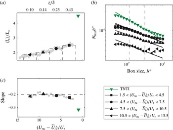
(a) The average length per unit streamwise length,
 $\langle l_{s}\rangle /L_{x}$
, of all UMZ edges at
 $Re_{\unicode[STIX]{x1D70F}}\approx 14\,500$
. Symbols are defined on the lower right. (b) Number of boxes
 $N_{box}$
needed to cover UMZ edges as a function of box size. The solid lines correspond to a power-law least-squares fit in range indicated by the vertical dashed lines. (c) Slope computed from the power-law fits in (b). The grey symbols in (a,c) correspond to results computed over a smaller momentum deficit range in steps of
 $(U_{\infty }-\widetilde{U}_{i})/U_{\unicode[STIX]{x1D70F}}=0.5$
.

Figure 6(a) shows
 $\langle l_{s}\rangle /L_{x}$
of all UMZ edges at varying momentum deficit ranges (
 ${\sim}$
wall-normal position). The results are presented for
 $Re_{\unicode[STIX]{x1D70F}}\approx 14\,500$
and
 $l_{s}$
is computed along a coordinate system attached to the interface. The black symbols correspond to results computed at internal interfaces in the momentum deficit ranges indicated by the vertical dashed lines, and the green ▾ symbol again represent results computed exclusively at the TNTI. The lowest momentum deficit range of
 $1.5<(U_{\infty }-\widetilde{U}_{i})/U_{\unicode[STIX]{x1D70F}}<4.5$
shows that on average, the length of interfaces within this range is approximately 2.5 times the streamwise domain length that it lies on. Thereafter, a reduction of this ratio is observed with increasing momentum deficit (closer proximity to the wall). The higher length of interfaces away from the wall may be caused by the increased presence of large-scale motions residing in this region, which in turn is likely to add large-scale bulges/valleys, increasing the ratio
 $\langle l_{s}\rangle /L_{x}$
. Such a scenario is consistent with the notion of larger length scales residing further away from the wall (e.g. Townsend Reference Townsend1976; Perry & Chong Reference Perry and Chong1982; Adrian et al.
Reference Adrian, Meinhart and Tomkins2000).
Our examination thus far exhibits a sharp rise in length at the TNTI (▾ symbols) relative to the edges of UMZs within the turbulent region. This trend can also be observed by visually inspecting instantaneous velocity fields (see figure 3
a), where a distinct increase in ‘wrinkles’ is present at the TNTI. We postulate that these differences between internal and external UMZ edges in boundary layers may be attributed to the different fluid ‘states’ present on either side of the edge. Across the TNTI, the fluid is turbulent on one side and non-turbulent on the other side, whereas turbulent fluid can be found either side of the internal UMZ boundaries/edges, albeit with differing intensities. Further, we speculate that entrainment of non-turbulent fluid via small-scale ‘nibbling’, may explain a sharp increase in
 $l_{s}$
due to an increase in surface area. To investigate this behaviour, the grey symbols show
 $l_{s}$
computed over smaller ranges of momentum deficit in steps of
 $(U_{\infty }-\widetilde{U}_{i})/U_{\unicode[STIX]{x1D70F}}=0.5$
. Again the results exhibit a distinct increase at the TNTI, albeit less converged, reaffirming our previous observations.
The presence of both large-scale bulges and finer wrinkles along the detected edges of UMZs motivates us to examine the multiscale characteristics of the interfaces. This would allow us to discern any degree of self-similarity across the range of scales present. Previously, studies have highlighted the geometric fractal behaviour of the TNTI (e.g. Sreenivasan & Meneveau Reference Sreenivasan and Meneveau1986; Siebesma & Jonker Reference Siebesma and Jonker2000), meanwhile, other studies have disputed these observations (e.g. Miller & Dimotakis Reference Miller and Dimotakis1991). However, recent works at high Reynolds numbers in turbulent boundary layers by de Silva et al. (Reference de Silva, Philip, Chauhan, Meneveau and Marusic2013) and also in jets by Mistry et al. (Reference Mistry, Philip, Dawson and Marusic2016) have confirmed a fractal dimension of
 ${\approx}2.3{-}2.4$
at the TNTI. Due to the comparably high
 $Re$
available in the present study, we examine whether similar fractal characteristics are present at the edges of UMZs within the turbulent region. We begin with a brief discussion on how the fractal dimension is computed using a box counting analysis (Prasad & Sreenivasan Reference Prasad and Sreenivasan1989, and others). First, each velocity field is divided into square boxes of a certain size,
 $b$
. Thereafter, we determine the number of boxes,
 $N_{box}$
, an interface lies on, which is then repeated for a range of box sizes across all available velocity fields. Finally, averaged statistics are computed over all velocity fields to determine if they exhibit a fractal behaviour following
 $N_{box}\sim b^{-D}$
, where
 $D$
represents the fractal dimension.
Figure 6(b) shows results for
 $N_{box}$
as a function of box size
 $b$
at
 $Re_{\unicode[STIX]{x1D70F}}\approx 14\,500$
. For clarity,
 $N_{box}$
is pre-multiplied by the box size
 $b$
to enable us to better discern any deviation from a log–log trend (
 $N_{box}\times b\sim b^{-D+1}$
). Further, we note that the largest box size is restricted by the fixed streamwise extent used to detect the presence of UMZs (
 ${\mathcal{L}}_{x}$
), however minimal influence on the computed fractal dimension was observed at different streamwise extents. The ▾ symbols correspond to the TNTI where a clear linear region is present with a slope of approximately
 $-0.3$
(solid line), or
 $D\approx 1.3$
. Consequently, one would obtain
 $D_{f}=D+1\approx 2.3$
for the surface embedded in three dimensions following the additive rule of co-dimensions (Mandelbrot Reference Mandelbrot1982). These results are in good quantitative agreement with previous findings at the TNTI (Sreenivasan & Meneveau Reference Sreenivasan and Meneveau1986; Meneveau & Sreenivasan Reference Meneveau and Sreenivasan1990; de Silva et al.
Reference de Silva, Philip, Chauhan, Meneveau and Marusic2013), across a wide range of detection schemes for the TNTI. Further, the magnitude of
 $D$
is also in agreement with recent findings of Borrell & Jiménez (Reference Borrell and Jiménez2016) from numerical simulations in turbulent boundary layers, who also examined the magnitude of
 $D$
across a wide range of vorticity thresholds used to detect the TNTI. We note the grey vertical dashed lines in figure 6(b) indicate conservative upper and lower bounds for the self-similar regions observed, so their precise magnitudes should not be taken as definitive estimates. Nevertheless, we observe a lower bound in figure 6(b) that is approximately below the Taylor microscale,
 $b<\unicode[STIX]{x1D706}_{T}$
. On the other hand at larger scales we again see a deviation, however, it is important to note that this upper limit is likely to be restricted by the streamwise extent of the databases and therefore the self-similar region may extend to even larger scales.
We can reproduce the same statistics at the edges of UMZs within the turbulent region, which are shown by the ▪, ●, ▴ and ◂ symbols in figure 6(b). Each symbol corresponds to statistics computed at different momentum deficit ranges (
 ${\sim}$
wall-normal locations) within the turbulent region, and they all appear to exhibit a linear behaviour of
 $\ln (N_{box}\times b^{+})$
as a function of
 $\ln (b^{+})$
. Therefore, similar to the TNTI we hypothesise that a fractal or self-similarity across a range of scales is prevalent at the internal interfaces that demarcate UMZs within the turbulent region. Upon closer inspection, it is evident that the fractal dimension, computed at UMZ edges within the turbulent region and the TNTI differs in magnitude. To better understand this behaviour, figure 6(c) presents the local slopes, computed from the profiles shown in figure 6(b). Here we observe a peculiar trend, where the slope (and subsequently fractal dimension
 $D$
) exhibits a nominally constant magnitude at UMZ edges within the turbulent region of
 $D\approx 1.2$
. However, at the TNTI we obtain a sharp change to
 $D\approx 1.3$
. We can, therefore, infer that both the TNTI and internal interfaces exhibit self-similarity across a range of scales, however, a lower fractal dimension for the internal interfaces is indicative of a smaller degree of contortions (both large-scale bulges/valleys and small-scale wrinkles). This is also evident from the sharp increase in interface length
 $l_{s}$
at the TNTI (see figure 6
a).
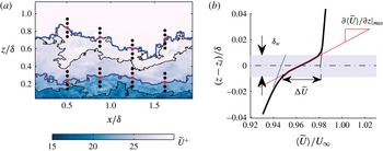
(a) Schematic on computing conditional statistics at UMZ edges overlaid on colour contours of streamwise velocity
 $\widetilde{U}$
. The solid black contours represent the original un-enveloped boundary, and the solid blue line corresponds to the ‘outer’ envelope of the boundary. The ● (red) symbols represent the coordinates
 $z_{i}$
along the interface and the ● symbols illustrate grid points collected in the near vicinity of each interface. (b) Averaged conditional statistics for the streamwise velocity,
 $\widetilde{U}$
, at the TNTI.
 $\unicode[STIX]{x0394}\widetilde{U}$
,
 $\unicode[STIX]{x1D6FF}_{w}$
and
 $\unicode[STIX]{x2202}\langle \widetilde{U}\rangle /\unicode[STIX]{x2202}z|_{max}$
correspond to the average jump in streamwise velocity, the width of the jump and the maximum local gradient of the profile, respectively.

4.3 Conditionally averaged statistics
So far we have examined geometric properties at the detected UMZ edges. In this section, we examine conditionally averaged statistical properties in the near vicinity of these UMZ edges using the same techniques commonly used to analyse interfacial layers in boundary layers (Westerweel et al.
Reference Westerweel, Fukushima, Pedersen and Hunt2009; Chauhan et al.
Reference Chauhan, Philip, de Silva, Hutchins and Marusic2014b
; Eisma et al.
Reference Eisma, Westerweel, Ooms and Elsinga2015). To perform this, a frame of reference attached to each interface at
 $z=z_{i}$
is used, as illustrated in figure 7(a). The subscript
 $i$
denotes a quantity computed at or along the interfaces, and the ● (red) symbols on figure 7 correspond to a few representative locations of the interface,
 $z_{i}$
. Thereafter, profiles of
 $\widetilde{U}$
,
 $\widetilde{W}$
and
 $\unicode[STIX]{x2202}\widetilde{U}/\unicode[STIX]{x2202}z$
are collected in the near vicinity of
 $z_{i}$
(● symbols on figure 7
a), which are averaged along the interface to obtain average conditional statistics (denoted by
 $\langle \rangle$
brackets). We note that most interfaces are heavily contorted and tend to fall back on themselves, therefore the ‘outer’ envelope of each interface is computed first, providing only a single possible wall-normal location at each streamwise grid point (Westerweel et al.
Reference Westerweel, Fukushima, Pedersen and Hunt2005; Kwon et al.
Reference Kwon, Philip, de Silva, Monty and Hutchins2014; Chauhan et al.
Reference Chauhan, Philip, de Silva, Hutchins and Marusic2014b
). This is illustrated in figure 7(a), where the black solid line (—) represents the original un-enveloped boundary, and the solid blue line (—) corresponds to the ‘outer’ envelope of the boundary. A careful examination of enveloping the interface to compute conditional statistics is described in Kwon et al. (Reference Kwon, Philip, de Silva, Monty and Hutchins2014), where negligible differences were found between the ‘inner’ or ‘outer’ envelope.
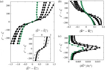
Figure 7(b) shows a conditionally averaged profile for
 $\widetilde{U}$
. The results are shown at the topmost UMZ edge (or TNTI), which reveals a sharp increase in the streamwise velocity of approximately 4 % of
 $U_{\infty }$
on average (denoted as
 $\unicode[STIX]{x0394}U$
), in agreement with previous findings at the TNTI (Chauhan et al.
Reference Chauhan, Philip, de Silva, Hutchins and Marusic2014b
; Eisma et al.
Reference Eisma, Westerweel, Ooms and Elsinga2015). We note that
 $\unicode[STIX]{x0394}U$
is computed by projecting linear fits to the regions above and below the sharp velocity change on the conditional wall-normal profile of
 $\widetilde{U}$
(see figure 7
b), following prior work on interfacial layers in boundary layers (Chauhan et al.
Reference Chauhan, Philip, de Silva, Hutchins and Marusic2014b
; Eisma et al.
Reference Eisma, Westerweel, Ooms and Elsinga2015). The shaded region corresponds to the spatial extent across which this sharp change in
 $\widetilde{U}$
occurs, and is denoted by
 $\unicode[STIX]{x1D6FF}_{w}$
(to be detailed further). Next, we examine these parameters at the edges of UMZs within the turbulent region.
Conditional wall-normal profiles of
 $\widetilde{U}$
,
 $\widetilde{W}$
and
 $\unicode[STIX]{x2202}\widetilde{U}/\unicode[STIX]{x2202}z$
of all UMZ edges are presented in figure 8(a–c), respectively. Statistics are collected and averaged at different momentum deficit ranges, and the subscript
 $i$
denotes statistics computed at
 $z_{i}$
, for example
 $\widetilde{U_{i}}$
and
 $\widetilde{W_{i}}$
corresponds to the streamwise and wall-normal velocity, respectively at the interface. All conditional statistics are computed with respect to the interface location
 $z_{i}$
as the wall-normal reference on the ordinate, and the mean interface velocities
 $\widetilde{U_{i}}$
and
 $\widetilde{W_{i}}$
are used as the abscissa reference in (a) and (b), respectively.
Conditionally averaged statistics of UMZ edges at
 $Re_{\unicode[STIX]{x1D70F}}\approx 14\,500$
with respect to the interface location
 $z_{i}$
. (a–c) correspond to
 $\langle \widetilde{U}\rangle$
,
 $\langle \widetilde{W}\rangle$
and the wall-normal shear
 $\unicode[STIX]{x2202}\langle \widetilde{U}\rangle /\unicode[STIX]{x2202}z$
, respectively. Results at UMZ edges within the turbulent region (internal interfaces) are binned by momentum deficit,
 $(U_{\infty }-\widetilde{U}_{i})/U_{\unicode[STIX]{x1D70F}}$
, and represented by different black symbols which are defined in figure 6. The green ▾ symbols correspond to results computed exclusively at the TNTI. The inset in (a) shows one standard deviation of the instantaneous
 $\widetilde{U}$
profiles for the ▴ symbols.

The results for the conditionally averaged streamwise velocity,
 $\langle \widetilde{U}\rangle$
, reveals a sharp increase in
 $\widetilde{U}$
when crossing the edge of UMZs (at
 $z-z_{i}=0$
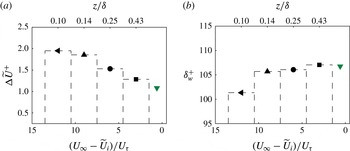
). This observation is in agreement with the notion that a large proportion of the shear present in boundary layers is concentrated over a small spatial extent, surrounded by relatively large regions of uniform streamwise momentum (see figure 4). Upon closer inspection, the profiles also reveal a higher
 $\unicode[STIX]{x0394}\widetilde{U}$
closer to the wall (higher momentum deficit), which is quantified in figure 9(a). These results are in agreement to those reported by Eisma et al. (Reference Eisma, Westerweel, Ooms and Elsinga2015) where an increase in velocity jump magnitude at interfacial layers of high shear were observed closer to the wall, with a comparable jump magnitude as a function of
 $z$
. Collectively, these findings emphasise the significance of the sharp changes in
 $\widetilde{U}$
(or
 $\unicode[STIX]{x0394}\widetilde{U}$
) computed at UMZ edges within the turbulent region, which has not received as much attention as the TNTI to date. The increase in
 $\unicode[STIX]{x0394}\widetilde{U}$
at larger momentum deficit (closer to the wall) is consistent with the mean flow characteristics of a turbulent boundary layer due to the higher mean velocity gradient in the near-wall region. Consequently, we postulate that the instantaneous
 $\widetilde{U}$
profile as a function of
 $z$
in turbulent boundary layers is predominantly composed of a step-like profile (zonal-like arrangement) with larger steps (or jumps in
 $\widetilde{U}$
) present on average in the near-wall region. Qualitative evidence of these postulations can be observed in arbitrarily chosen instantaneous velocity profiles (see figure 1), or by visually inspecting
 $\unicode[STIX]{x2202}\widetilde{U}/\unicode[STIX]{x2202}z$
contours (see figure 3
b), where the magnitude of
 $\unicode[STIX]{x2202}\widetilde{U}/\unicode[STIX]{x2202}z$
is higher closer to the wall.
So far the conditional profiles of
 $\widetilde{U}$
presented in figure 8(a) quantifies the average behaviour, however, instantaneously
 $\widetilde{U}$
fluctuates significantly near UMZ edges (see figure 1). In an attempt to quantify this, the dashed lines in the inset of figure 8(a) shows one standard deviation of the
 $\widetilde{U}$
profiles for the ▴ symbols. Although not reproduced here, the other momentum deficit ranges (
 ${\sim}$
wall-normal locations) exhibit similar behaviour. Figure 8(b) reproduces the same conditional statistics for the wall-normal velocity component near UMZ edges. The results reveal that the sharp increase in the streamwise velocity at the edge of UMZs for increasing
 $(z-z_{i})$
is flanked by a decrease in the wall-normal velocity, albeit more gradual. Such a scenario is consistent with the signature of
 $Q2$
(
 $\widetilde{U}<0$
,
 $\widetilde{W}>0$
) events below UMZ edges and
 $Q4$
(
 $\widetilde{U}>0$
,
 $\widetilde{W}<0$
) events above UMZ edges, relative to the streamwise (
 $\widetilde{U_{i}}$
) and wall-normal (
 $\widetilde{W_{i}}$
) velocity at the interface i.e. consistent with the VITA event, of a stagnation point residing upstream of the head of a hairpin vortex (Adrian et al.
Reference Adrian, Meinhart and Tomkins2000).
(a) The average jump in streamwise velocity,
 $\unicode[STIX]{x0394}\widetilde{U}^{+}$
, (b) width across which it occurs,
 $\unicode[STIX]{x1D6FF}_{w}^{+}$
, computed from the conditionally averaged statistics at UMZ edges at
 $Re_{\unicode[STIX]{x1D70F}}\approx 14\,500$
. Detected UMZ edges are binned by momentum deficit (
 $(\widetilde{U}_{i}-U_{\infty })/U_{\unicode[STIX]{x1D70F}}$
) with the range indicated by the dashed lines, and also by different symbols which are defined in figure 6. The green ▾ symbols correspond to results computed exclusively at the TNTI.

Next, we examine the spatial extent across which we observe a sharp change in streamwise velocity, here denoted as
 $\unicode[STIX]{x1D6FF}_{w}$
. Due to the qualitative similarity between conditional profiles obtained for the TNTI and at the edges of UMZs, we estimate
 $\unicode[STIX]{x1D6FF}_{w}$
based on prior work at the TNTI. Specifically,
 $\unicode[STIX]{x1D6FF}_{w}$
is computed following Brown & Roshko (Reference Brown and Roshko1974), Chauhan et al. (Reference Chauhan, Philip, de Silva, Hutchins and Marusic2014b
) as
 $$\begin{eqnarray}\displaystyle \unicode[STIX]{x1D6FF}_{w}=\frac{\unicode[STIX]{x0394}\widetilde{U}}{\unicode[STIX]{x2202}\langle \widetilde{U}\rangle /\unicode[STIX]{x2202}z|_{max}}, & & \displaystyle\end{eqnarray}$$
where
 $\unicode[STIX]{x0394}\widetilde{U}$
and
 $\unicode[STIX]{x2202}\langle \widetilde{U}\rangle /\unicode[STIX]{x2202}z|_{max}$
correspond to the average jump in streamwise velocity, and the maximum local gradient of the profile, respectively (see figure 7
b). Estimates of
 $\unicode[STIX]{x1D6FF}_{w}$
are presented in figure 9(b), showing a slight reduction of
 $\unicode[STIX]{x1D6FF}_{w}$
with increasing momentum deficit (decreasing distance from the wall). One possible basis for this trend could be the presence of larger diameter vortices residing further away from the wall. Such a postulation is in agreement with certain physical models for boundary layers and prior experimental evidence (Perry & Chong Reference Perry and Chong1982; Adrian et al.
Reference Adrian, Meinhart and Tomkins2000; Herpin et al.
Reference Herpin, Stanislas, Foucaut and Coudert2013; Morrill-Winter & Klewicki Reference Morrill-Winter and Klewicki2013, and others). Alternatively, a more probable explanation for the slight increase in
 $\unicode[STIX]{x1D6FF}_{w}$
we observe as a function of
 $z$
could be caused by the proportion of high shear and low shear regions present along UMZ edges. Qualitative evidence of this change in the proportion of high/low shear regions along internal interfaces can be observed on the shear fields, such as the one shown in figure 3(b), where the high shear regions (dark shading) increase in sparsity with increasing
 $z$
. As a consequence, the increased prevalence of low shear regions along the edges of UMZ further away from the wall may attenuate the magnitude of
 $\unicode[STIX]{x2202}\langle \widetilde{U}\rangle /\unicode[STIX]{x2202}z|_{max}$
(or increase
 $\unicode[STIX]{x1D6FF}_{w}$
) with increasing
 $z$
. It is also worth noting that the spatial resolution of the measurement (the interrogation window size in our case) is likely to influence the velocity gradient across each interface and the subsequent estimate of
 $\unicode[STIX]{x1D6FF}_{w}$
. Thus, we can consider the computed
 $\unicode[STIX]{x1D6FF}_{w}$
to be an upper bound, with some uncertainty as to its exact value. We also note that our results are comparable to
 $\unicode[STIX]{x1D6FF}_{w}$
estimates from interfacial layers of high shear in boundary layers by Eisma et al. (Reference Eisma, Westerweel, Ooms and Elsinga2015), who used a database with twice the spatial resolution. As a final note, our results also reveal the largest
 $\unicode[STIX]{x1D6FF}_{w}$
at the TNTI with a magnitude similar to that previously reported by Chauhan et al. (Reference Chauhan, Philip, de Silva, Hutchins and Marusic2014b
), albeit using different detection criteria. Therefore, the magnitude of
 $\unicode[STIX]{x1D6FF}_{w}$
appears to be somewhat robust to different TNTI detection criteria.
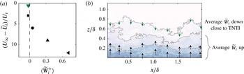
Now we focus our attention on the wall-normal velocity at the interface,
 $\langle \widetilde{W_{i}}\rangle$
. Results are shown in figure 10(a), which exhibits an increasingly positive magnitude for
 $\langle \widetilde{W_{i}}\rangle$
closer to the wall, conversely at the TNTI
 $\langle \widetilde{W_{i}}\rangle$
is slightly negative. One possible explanation for this trend may be made with reference to the streamwise evolution of a boundary layer, where we observe increasing momentum deficit close to the wall (with increasing
 $x$
). This, in turn, would push mass away from the wall as a turbulent boundary layer develops (positive
 $\widetilde{W_{i}}$
) on average. If we turn our attention to the TNTI (top edge of UMZ furthest away from the wall),
 $\langle \widetilde{W_{i}}\rangle$
is negative, which is in agreement with the notion that at the TNTI mass from the non-turbulent region is entrained into the turbulent region (see also Chauhan, Philip & Marusic (Reference Chauhan, Philip and Marusic2014a
), Chauhan et al. (Reference Chauhan, Philip, de Silva, Hutchins and Marusic2014b
), Eisma et al. (Reference Eisma, Westerweel, Ooms and Elsinga2015), which discusses the conditionally averaged wall-normal velocity at the TNTI). As a consequence, we now have two competing mechanisms (entrainment at TNTI and the mass pushed up from the near near-wall region). Therefore
 $\langle \widetilde{W_{i}}\rangle$
is likely to undergo a sign change in the wake region, which appears in figure 10(a) and is also qualitatively illustrated in figure 10(b). Based on such a scenario in conjunction with the streamwise growth rate of the boundary layer, we may hypothesise that the structures responsible for the presence of UMZs encapsulated by high shear regions are growing/moving away from the wall on average. This would be in agreement with findings at interfacial layers of high shear in boundary layers which were reported by Eisma et al. (Reference Eisma, Westerweel, Ooms and Elsinga2015) to move away from the wall. However to confirm this, temporally resolved databases would be required to track the edges of UMZs, which are unavailable in this study.
(a) Conditionally averaged wall-normal velocity,
 $\langle \widetilde{W}\rangle$
at UMZ edges. Results are presented at
 $Re_{\unicode[STIX]{x1D70F}}\approx 14\,500$
and are computed at the interface/edge location,
 $z_{i}$
. The vertical dashed line corresponds to
 $\langle \widetilde{W}\rangle =0$
, and the symbols are as defined in figure 6. (b) Schematic of
 $\langle \widetilde{W}\rangle$
at UMZ edges overlaid on colour contours of streamwise velocity
 $\widetilde{U}$
. The black and green arrows correspond to UMZ edges within the turbulent region and the TNTI, respectively.

5 Influence of Reynolds number and scaling
This study employs databases across a large range of Reynolds numbers spanning over a decade, therefore we now turn our attention to examine characteristic parameters at UMZ edges previously discussed, as a function of
 $Re$
. From this analysis we aim to examine scaling of these parameters based on experimental evidence and theoretical reasoning.
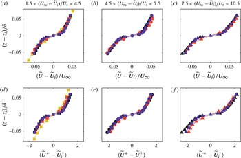
Conditionally averaged streamwise velocity profiles in the near vicinity of all detected internal interfaces, normalised by (a–c)
 $U_{\infty }$
and (d–f)
 $U_{\unicode[STIX]{x1D70F}}$
. Each vertical column (and its associated symbol) corresponds to different momentum deficit ranges (
 ${\sim}$
wall-normal location), where (a,d)
 $1.5<(U_{\infty }-\widetilde{U}_{i})/U_{\unicode[STIX]{x1D70F}}<4.5$
, (b,e)
 $4.5<(U_{\infty }-\widetilde{U}_{i})/U_{\unicode[STIX]{x1D70F}}<7.5$
and (c,f)
 $7.5<(U_{\infty }-\widetilde{U}_{i})/U_{\unicode[STIX]{x1D70F}}<10.5$
. The darker symbols correspond to higher Reynolds numbers (e.g. on the left column the ● (yellow), ● (red), ● (blue) and ● (black) symbols correspond to datasets at
 $Re_{\unicode[STIX]{x1D70F}}\approx 1200$
,
 $Re_{\unicode[STIX]{x1D70F}}\approx 2800$
,
 $Re_{\unicode[STIX]{x1D70F}}\approx 8000$
and
 $Re_{\unicode[STIX]{x1D70F}}\approx 14\,500$
, respectively.)

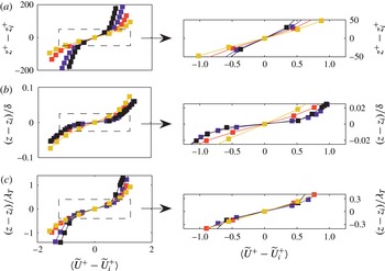
Conditionally averaged streamwise velocity profiles in the near-vicinity of all detected internal interfaces within the momentum deficit range
 $1.5<(U_{\infty }-\widetilde{U}_{i})/U_{\unicode[STIX]{x1D70F}}<4.5$
. Length scales (ordinate) are normalised by (a) viscous units, (b) boundary layer thickness
 $\unicode[STIX]{x1D6FF}$
and (c) Taylor microscale
 $\unicode[STIX]{x1D706}_{T}$
. Colour shading and symbols are defined in figure 11. The right hand column shows magnified views across the wall-normal extent of the sharp change in
 $\widetilde{U}$
.

5.1 Velocity and length scales
Previously, figure 8(a) showed conditional statistics computed on a frame of reference attached to each interface, which revealed a persistent sharp rise in streamwise velocity,
 $\unicode[STIX]{x0394}\widetilde{U}$
across a finite thickness,
 $\unicode[STIX]{x1D6FF}_{w}$
. The results in figure 11 reproduces the same statistics now computed across all four experimental databases. Again all results are presented on a frame of reference attached to each interface at
 $z_{i}$
. Each column in figure 11 represents a different momentum deficit range. We note that conditional statistics at the higher deficit ranges are unavailable for the lower
 $Re$
databases due to the lack of near-wall data. To examine the appropriate velocity scales, the rows of figure 11(a–f) present conditional statistics normalised by
 $U_{\infty }$
and
 $U_{\unicode[STIX]{x1D70F}}$
, respectively. The results show good qualitative collapse over the range of Reynolds numbers considered, with no discernible difference between scaling the profiles by
 $U_{\infty }$
or
 $U_{\unicode[STIX]{x1D70F}}$
. We note that both
 $U_{\infty }$
and
 $U_{\unicode[STIX]{x1D70F}}$
are weak functions of
 $Re_{\unicode[STIX]{x1D70F}}$
, therefore, an even larger
 $Re$
range would be necessary to fully examine the appropriate velocity scale. Nevertheless, an attempt to quantify the appropriate velocity scale based on these qualitative observations are presented later in this work (see figure 13
a,b). We also note that a more rational explanation for scaling with
 $U_{\unicode[STIX]{x1D70F}}$
has been provided by Chauhan et al. (Reference Chauhan, Philip and Marusic2014a
), albeit only for the TNTI.
Next, we turn our attention to the length scales prevalent at the UMZ edges. To this end, figure 12 shows conditional statistics with the length scale on the ordinate normalised by (a) viscous units, (b) the boundary layer thickness and (c) the Taylor microscale. We note results are only shown for a single momentum deficit range (
 $1.5<(U_{\infty }-\widetilde{U}_{i})/U_{\unicode[STIX]{x1D70F}}<4.5$
), however, other momentum deficit ranges also show similar behaviour and are not reproduced here for brevity. Figure 12(a) presents normalisation of length scales by viscous units, revealing poor collapse for the
 $Re$
range examined. Similar observations are also present when normalised by the boundary layer thickness,
 $\unicode[STIX]{x1D6FF}$
(see zoomed region of figure 12
b). On the other hand, the zoomed region of figure 12(c) reveals that normalisation by the Taylor microscale,
 $\unicode[STIX]{x1D706}_{T}$
, exhibits improved agreement. An attempt to quantify these qualitative observations on the prevalent velocity and length scales will follow next.
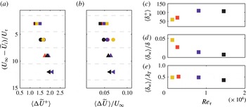
Accordingly, figure 13 shows a collection of characteristic properties of the conditional statistics as a function of
 $Re$
. Specifically, we examine the magnitude of the sharp change in streamwise velocity,
 $\unicode[STIX]{x0394}\widetilde{U}$
, and thickness across which it occurs,
 $\unicode[STIX]{x1D6FF}_{w}$
, in (a,b) and (c–e), respectively. This enables us to quantify some of the qualitative observations from figures 11 and 12. We note that the parameters
 $\unicode[STIX]{x0394}\widetilde{U}$
and
 $\unicode[STIX]{x1D6FF}_{w}$
are computed based on functional fits to conditional statistics (see figure 7), therefore precise numerical values for these characteristic properties must be taken with some degree of caution. Figure 13(a,b) show
 $\unicode[STIX]{x0394}\widetilde{U}$
computed across the entire extent of the boundary layer as a function of
 $Re$
normalised by
 $U_{\unicode[STIX]{x1D70F}}$
and
 $U_{\infty }$
, respectively. Although visual inspection of conditional profiles of
 $\widetilde{U}$
in the near vicinity of the interface (see figure 11) showed no discernible difference between scaling by
 $U_{\unicode[STIX]{x1D70F}}$
and
 $U_{\infty }$
, the results in figure 13(a) exhibits slightly better agreement is attained for
 $U_{\unicode[STIX]{x1D70F}}$
, albeit from a functional fit. Nevertheless, this result is in agreement with the fact that
 $U_{\unicode[STIX]{x1D70F}}$
serves as the appropriate velocity scale for the mean velocity deficit and the turbulent stresses in the outer region (Tennekes & Lumley Reference Tennekes and Lumley1972). Additionally, prior work has reported that the sharp change in
 $\widetilde{U}$
across the TNTI in turbulent boundary layers also exhibits invariance when scaled with
 $U_{\unicode[STIX]{x1D70F}}$
(Chauhan et al.
Reference Chauhan, Philip, de Silva, Hutchins and Marusic2014b
). Therefore, our findings extend this behaviour to the edges of UMZs within the turbulent region, allowing us to infer that both the external (TNTI) and internal UMZ edges in boundary layers have turbulent motions with velocities that scale with the friction velocity.
Characteristic properties computed from conditional profiles in the near vicinity of the edges of UMZs. (a,b) The average jump in streamwise velocity,
 $\unicode[STIX]{x0394}\widetilde{U}^{+}$
, normalised by
 $U_{\unicode[STIX]{x1D70F}}$
and
 $U_{\infty }$
, respectively. (c–e) The width across which the jump occurs,
 $\unicode[STIX]{x1D6FF}_{w}$
, normalised by
 $U_{\unicode[STIX]{x1D70F}}$
,
 $\unicode[STIX]{x1D6FF}$
and
 $\unicode[STIX]{x1D706}_{T}$
, respectively. Results in (c–e) are computed for UMZ edges in the momentum deficit range
 $1.5<(U_{\infty }-\widetilde{U}_{i})/U_{\unicode[STIX]{x1D70F}}<4.5$
.

Next, we attempt to quantify the width,
 $\unicode[STIX]{x1D6FF}_{w}$
, across which the sharp change in streamwise velocity occurs as a function of
 $Re$
. To this end, figure 13(c) presents
 $\unicode[STIX]{x1D6FF}_{w}$
normalised with
 $\unicode[STIX]{x1D708}/U_{\unicode[STIX]{x1D70F}}$
as the length scale. The results show an increase in
 $\unicode[STIX]{x1D6FF}_{w}^{+}$
at low
 $Re$
which seems to plateau to an asymptotic limit as
 $Re$
increases. This behaviour at high
 $Re$
is encouraging as it is in close agreement with prior findings at the TNTI (Chauhan et al.
Reference Chauhan, Philip and Marusic2014a
). Therefore, we may infer similarity between both length and velocity scales of turbulent motions at all edges of UMZs (inclusive of the TNTI) in boundary layers. Further similarities to the TNTI are also exhibited for normalisation of
 $\unicode[STIX]{x1D6FF}_{w}$
as a fraction of boundary layer thickness (
 $\unicode[STIX]{x1D6FF}$
) and the Taylor microscale
 $\unicode[STIX]{x1D706}_{T}$
, which are shown in figure 13(c,d), respectively. Specifically, normalisation of the width by
 $\unicode[STIX]{x1D6FF}$
exhibits that the high shear regions present at UMZ edges are thinner relative to
 $\unicode[STIX]{x1D6FF}$
at higher
 $Re$
, which is in agreement with visual inspections of the instantaneous shear at different
 $Re$
(see figure 3). On the other hand,
 $\unicode[STIX]{x1D6FF}_{w}$
normalisation by
 $\unicode[STIX]{x1D706}_{T}$
reveals improved invariance with
 $Re$
which is in agreement with qualitative evidence previously shown in figure 12. As a consequence, the width of the internal interfaces appear to be
 $O(\unicode[STIX]{x1D706}_{T})$
. Similar observations were also reported by Eisma et al. (Reference Eisma, Westerweel, Ooms and Elsinga2015) at a fixed
 $Re$
across a range of wall-normal locations.
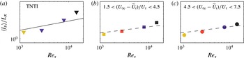
The average length (
 $l_{s}$
) per unit streamwise length (
 ${\mathcal{L}}_{x}$
) computed from all experimental datasets. (a) Corresponds to the statistics computed exclusively at the TNTI. (b,c) correspond to edges of UMZs within the momentum deficit ranges (
 ${\sim}$
wall-normal location)
 $1.5<(U_{\infty }-\widetilde{U}_{i})/U_{\unicode[STIX]{x1D70F}}<4.5$
and
 $4.5<(U_{\infty }-\widetilde{U}_{i})/U_{\unicode[STIX]{x1D70F}}<7.5$
, respectively. Symbols correspond to different datasets and are defined in figure 11. The solid line in (a) and dashed lines in (b,c) correspond to a power-law fit with a slope of 0.225 and 0.15, respectively.

If we turn our attention to the surrounding regions away from the UMZ edge (
 $z\ll z_{i}$
or
 $z\gg z_{i}$
), or the UMZs themselves, the results show the best agreement when scaled with
 $\unicode[STIX]{x1D6FF}$
(see figure 12
b). Therefore, we may postulate that the appropriate length scales for the structures associated with the UMZs are
 $O(\unicode[STIX]{x1D6FF})$
(see de Silva et al.
Reference de Silva, Hutchins and Marusic2016). Collectively, a possible explanation for the lengths scales observed both within UMZs (
 $O(\unicode[STIX]{x1D6FF})$
) and at their associated edges (
 $O(\unicode[STIX]{x1D706}_{T})$
) can be postulated following Sreenivasan, Ramshankar & Meneveau (Reference Sreenivasan, Ramshankar and Meneveau1989) (also see da Silva & Taveira Reference da Silva and Taveira2010), where the time scale,
 $T$
, over which the large structures act is
 $(\unicode[STIX]{x1D6FF}/U_{\unicode[STIX]{x1D70F}})$
. Here,
 $U_{\unicode[STIX]{x1D70F}}$
is the relevant turbulent velocity scale across the turbulent boundary layer. During this time,
 $T$
, the viscous diffusion will act over a distance
 $$\begin{eqnarray}\displaystyle l_{vis}\approx \sqrt{\unicode[STIX]{x1D708}T}=\sqrt{\unicode[STIX]{x1D708}\unicode[STIX]{x1D6FF}/U_{\unicode[STIX]{x1D70F}}}\Rightarrow \frac{l_{vis}}{\unicode[STIX]{x1D6FF}}\sim \frac{1}{\sqrt{Re_{\unicode[STIX]{x1D70F}}}}, & & \displaystyle\end{eqnarray}$$
and consequently
 $l_{vis}\sim \unicode[STIX]{x1D706}$
(e.g. Tennekes & Lumley Reference Tennekes and Lumley1972).
5.2 Scaling of geometric properties
An examination of the average interface length
 $l_{s}$
as a function of
 $Re$
is presented in figure 14(a), which shows results computed exclusively at the TNTI. Figure 14(b,c) reproduces the same statistics for the UMZ edges within the turbulent region at two different momentum deficit ranges (
 ${\sim}$
wall-normal locations). At the TNTI we observe an increase in
 $l_{s}$
with
 $Re$
, which can be attributed to the increased range of scales present at high
 $Re$
that leads to a more convoluted TNTI. A similar behaviour is also observed at the edges of the UMZs within the turbulent region shown in figure 14(b,c), albeit with a smaller slope (slower increase in
 $l_{s}$
with
 $Re$
for the internal interfaces as compared to the TNTI). This slower increase in
 $l_{s}$
with
 $Re$
for the internal interfaces is in agreement with the observed differences in fractal dimension between internal shear layers and the TNTI as reported in § 4.2.
Accordingly, the
 $Re$
variation of the lengths presented in figure 14 can be estimated based on the self-similar nature of the fractal scaling. At a particular
 $Re$
the length of the interface scales like
 $l_{s}\sim b^{-D+1}$
for a given scale
 $b$
, where
 $D\approx 1.3$
and
 $1.2$
for the TNTI and the internal interfaces, respectively (see figure 6). If we assume that there is no variation to the length below the Kolmogorov length scale
 $\unicode[STIX]{x1D702}$
, then the length reported in figure 14 follows
 $$\begin{eqnarray}\displaystyle l_{s}(\unicode[STIX]{x1D702})=\langle l_{s}\rangle \sim \unicode[STIX]{x1D702}^{-D+1}. & & \displaystyle\end{eqnarray}$$
Additionally, it is evident that the largest cut-off of the power-law scaling is likely to be at a constant fraction of
 $\unicode[STIX]{x1D6FF}$
(e.g. de Silva et al.
Reference de Silva, Philip, Chauhan, Meneveau and Marusic2013), suggesting
 $$\begin{eqnarray}\displaystyle \langle l_{s}\rangle /l_{s}(\unicode[STIX]{x1D6FF})\sim (\unicode[STIX]{x1D702}/\unicode[STIX]{x1D6FF})^{-D+1}. & & \displaystyle\end{eqnarray}$$
Now,
 $\unicode[STIX]{x1D702}/\unicode[STIX]{x1D6FF}\sim Re_{\unicode[STIX]{x1D70F}}^{-3/4}$
and
 $l_{s}(\unicode[STIX]{x1D6FF})\sim L_{x}$
, which result in
 $$\begin{eqnarray}\displaystyle \langle l_{s}\rangle /L_{x}\sim Re_{\unicode[STIX]{x1D70F}}^{-3/4(-D+1)}. & & \displaystyle\end{eqnarray}$$
This suggests,
 $$\begin{eqnarray}\frac{\langle l_{s}\rangle }{L_{x}}\sim Re_{\unicode[STIX]{x1D70F}}^{0.225},\quad \text{for the TNTI},\quad \text{and}\quad \frac{\langle l_{s}\rangle }{L_{x}}\sim Re_{\unicode[STIX]{x1D70F}}^{0.15}\quad \text{for internal interfaces.}\qquad\end{eqnarray}$$
These two scalings are shown by solid and dashed lines in figure 14(a–c), respectively, and exhibit reasonable agreement with the data over a decade in
 $Re$
.
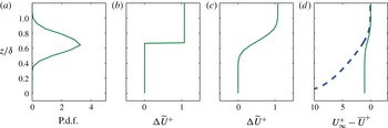
(a) The p.d.f. of the wall-normal location of the TNTI,
 $z_{i}$
, at
 $Re_{\unicode[STIX]{x1D70F}}\approx 14\,500$
. (b) Velocity jump
 $\unicode[STIX]{x0394}\widetilde{U}^{+}$
(see § 4.3) in streamwise velocity at TNTI modelled as a step function. (c) Resultant velocity profile from convolving (a,b). (d) Velocity deficit of the modelled profile,
 $U_{\infty ,m}^{+}-\overline{U}_{m}^{+}$
(solid line) in (c) overlaid on the mean velocity deficit,
 $U_{\infty }^{+}-\overline{U}^{+}$
(dashed blue line).

Modelled results in figure 15 reproduced for all UMZ edges at
 $Re_{\unicode[STIX]{x1D70F}}\approx 14\,500$
. (a) P.d.f. of
 $z_{i}$
, where the dashed line corresponds to the TNTI (same as figure 15
a), and each solid line corresponds to UMZ edges within the turbulent region. The solid lines correspond to five equispaced momentum deficit ranges within the bounds
 $1<(U_{\infty }-\widetilde{U}_{i})/U_{\unicode[STIX]{x1D70F}}<10$
. (b) The corresponding velocity jumps,
 $\unicode[STIX]{x0394}\widetilde{U}^{+}$
, modelled as step functions. (c) Velocity profiles from convolving the corresponding profiles in (a,b). (d) Mean velocity profile,
 $\overline{U}_{m}^{+}$
, obtained by the superposition of the profiles in (c). (e) Dotted line: modelled mean velocity deficit,
 $U_{\infty ,m}^{+}-\overline{U}_{m}^{+}$
, dashed line: mean velocity deficit,
 $U_{\infty }^{+}-\overline{U}^{+}$
, from the same database. (f) Mean velocity profiles as a function of
 $z^{+}$
corresponding to the deficit profiles in (e).

Modelled results for the mean flow computed at (a)
 $Re_{\unicode[STIX]{x1D70F}}\approx 2500$
from a DNS databases of Sillero, Jiménez & Moser (Reference Sillero, Jiménez and Moser2013), (b)
 $Re_{\unicode[STIX]{x1D70F}}\approx 2800$
and (c)
 $Re_{\unicode[STIX]{x1D70F}}\approx 8000$
. ● symbols: modelled mean velocity profile,
 $\overline{U}_{m}^{+}$
, dashed line: mean velocity profile,
 $\overline{U}^{+}$
, from the same database.

6 Towards reconstructing the mean velocity profile from the statistical behaviour of instantaneous profiles
The preceding discussions have highlighted the prevalence of a zonal-like structural arrangement in turbulent boundary layers. As a consequence, we have seen that instantaneous wall-normal profiles of
 $\widetilde{U}$
as a function of wall-normal height are populated by sharp changes in momentum flanked by regions of nominally uniform momentum. It then follows to examine how the instantaneous structural composition of the boundary layer (a zonal-like structure) manifests itself in the temporally averaged mean velocity profile.
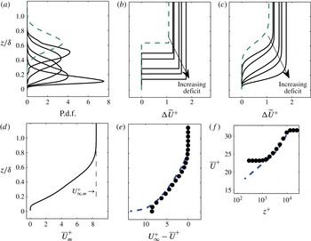
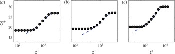
To construct the mean velocity profile, we envisage that the boundary layer profile has many step-like changes in momentum (in a conditional sense), which are ‘flapping’ around in the wall-normal direction (see figure 5 b). Therefore, once each step change in momentum (or UMZ edge) is arranged based on a p.d.f. of its wall-normal location we would obtain an estimate of its contribution to the mean velocity profile. To illustrate this procedure we shall consider the step change at the TNTI as an example, and subsequently apply the same procedure to the other steps (or UMZ edges) within the turbulent region to obtain an estimate of the mean velocity profile.
The probability distribution of the instantaneous wall-normal location of the TNTI shown in figure 15(a) is used as a measure on how the sharp change in streamwise velocity at the TNTI,
 $\unicode[STIX]{x0394}\widetilde{U}$
, flutters across a wide range of wall-normal locations. Additionally, in § 4.3 we evidenced that
 $\unicode[STIX]{x0394}\widetilde{U}$
at the TNTI occurs over a small wall-normal extent,
 $\unicode[STIX]{x1D6FF}_{w}$
, where
 $\unicode[STIX]{x1D6FF}_{w}/\unicode[STIX]{x1D6FF}\rightarrow 0$
at high
 $Re$
. As a consequence, we propose that
 $\unicode[STIX]{x0394}\widetilde{U}$
can be modelled a step function, which is illustrated in figure 15(b). Here the magnitude of
 $\unicode[STIX]{x0394}\widetilde{U}$
is determined from conditional statistics at the TNTI following the procedure outlined in § 4.3, and its reference location is chosen to be the mean interface location (
 $z/\unicode[STIX]{x1D6FF}\approx 2/3$
). Thereafter, the resultant velocity distribution (see figure 15
c) is obtained by convolving the step profile in figure 15(b) and the p.d.f. of
 $z_{i}$
in figure 15(a) – an approach outlined previously in works exclusively at the TNTI (Westerweel et al.
Reference Westerweel, Fukushima, Pedersen and Hunt2005; Chauhan et al.
Reference Chauhan, Philip and Marusic2014a
,Reference Chauhan, Philip, de Silva, Hutchins and Marusic
b
), and also described recently in the work of Krug, philip & Marusic (Reference Krug, philip and Marusic2017) to interpret the wake component in wall-bounded flows. The ensuing modelled profile is shown in figure 15(d) in velocity deficit form, and shows good collapse in the region
 $z/\unicode[STIX]{x1D6FF}>0.85$
against the temporally averaged velocity deficit (dashed blue line) from the same database. Better agreement deeper into the boundary layer could be attained by modelling the step-like changes in momentum within the turbulent region evidenced in this work. To this end, we incorporate quantitative measures discussed in § 4.3.
First, an estimate of the average number of UMZ edges (
 ${\sim}$
number of momentum deficit ranges) for a given
 $Re$
is necessary. Previously, we chose to examine momentum deficit ranges which remain fixed for all databases, since it was primarily used as a surrogate marker for wall-normal location and also simplified examining a wide range of
 $Re$
. However, for the present case we examine a single representative database at
 $Re_{\unicode[STIX]{x1D70F}}\approx 14\,500$
, therefore, the number of UMZ edges are inferred from the average number of UMZs reported by de Silva et al. (Reference de Silva, Hutchins and Marusic2016) at an equivalent
 $Re$
. Specifically, their work showed that approximately five UMZs are present on average, therefore we anticipate the presence of six UMZ edges (inclusive of the TNTI as the topmost UMZ edge) across the momentum deficit range available (above
 $z^{+}>200$
).
Figure 16(a) shows the distributions of
 $z_{i}$
for such a scenario, where the six profiles correspond to each of the UMZ edges present on average. The dashed line corresponds to statistics computed exclusively at the TNTI (same as figure 15), meanwhile the solid lines correspond to UMZ edges within the turbulent region. For simplicity, the five solid lines are computed by binning the internal interfaces into equispaced momentum deficit ranges within the bounds
 $1<(U_{\infty }-\widetilde{U}_{i})/U_{\unicode[STIX]{x1D70F}}<10$
. We note that including a larger deficit range allows us to model an even greater wall-normal extent; however conditional statistics (see figure 8) at UMZ edges closer to the wall are unavailable due to the lack of near-wall data. This shortcoming is also evident in figure 16(a), where the probability tends to zero below
 $z/\unicode[STIX]{x1D6FF}\lesssim 0.05$
. Each p.d.f. presented in figure 16(a) has a corresponding step change in velocity,
 $\unicode[STIX]{x0394}\widetilde{U}$
, which is shown in figure 16(b). The magnitude of
 $\unicode[STIX]{x0394}\widetilde{U}$
for each profile is computed from the procedure outlined in § 4.3. Thereafter, a convolution of the step-like profiles in figure 16(b) with their corresponding p.d.f. of
 $z_{i}$
in figure 16(a) provides the resultant velocity distribution for each momentum deficit range, which is presented in figure 16(c).
Next, a summation of the velocity distributions in figure 16(c) provides an estimate of the modelled mean velocity profile,
 $\overline{U}_{m}^{+}$
, which is presented in figure 16(d). The dotted line in figure 16(e) presents
 $\overline{U}_{m}^{+}$
in defect form (
 $U_{\infty ,m}^{+}-\overline{U}_{m}^{+}$
), which is overlaid on the actual velocity deficit (dashed blue line) from the same database. The two profiles exhibit encouraging agreement throughout the wall-normal extent available. The same procedure is repeated for the other experimental databases and also on a recent direct numerical simulation (DNS) database at
 $Re_{\unicode[STIX]{x1D70F}}\approx 2500$
(Sillero et al.
Reference Sillero, Jiménez and Moser2013), at matched conditions (see de Silva et al. (Reference de Silva, Hutchins and Marusic2016) for further details). The results are shown in figure 17, and again we observe encouraging agreement. Even better agreement might have been obtained with improved estimates of
 $\unicode[STIX]{x0394}\widetilde{U}$
or with additional near-wall information. Further, the shallow velocity gradient (or variation) within the UMZs themselves surrounding
 $\unicode[STIX]{x0394}\widetilde{U}$
, which is increasingly prevalent closer to the wall (see figure 8
a), is also neglected. Nevertheless, the present model is a first step towards constructing the mean velocity profile from the step-like instantaneous velocity profiles. Additionally, it affords strong support that sudden step-like changes in instantaneous velocity profiles, with an observed distribution in wall-normal location, can lead to the temporally averaged mean profile and even give a hint of the logarithmic velocity profile (see figure 16
f).
7 Summary and concluding remarks
Through the use of experimental datasets which span over a decade of friction Reynolds numbers, we investigate the structural properties of thin interfacial layers at which sharp changes in momentum occur across the entire extent of the turbulent boundary layer. The study begins with a description of a detection criteria used previously to locate regions of uniform streamwise momentum (or UMZs) based on the probability density histograms of the streamwise velocity (see Adrian et al. Reference Adrian, Meinhart and Tomkins2000; de Silva et al. Reference de Silva, Hutchins and Marusic2016). Thereafter, by means of a simple extension, we show how this criterion can be employed to estimate the spatial location of the edges that demarcate UMZs, which is the focus of the present study.
Our analysis reveals the geometry of the interfacial layers that separate UMZs in the turbulent region are highly contorted over a wide range of scales. Consequently, they exhibit average lengths that are significantly longer than the streamwise extent they lie upon. Further, a power-law scaling is observed at all UMZ edges with a near-constant fractal dimension throughout the turbulent region. This reveals a degree of self-similarity across a wide range of scales present at UMZ edges. A similar investigation at the turbulent/non-turbulent interface also exhibited a high degree of contortion and fractal scaling. Evidence is presented that the fractal dimension undergoes a sudden increase between UMZ edges within the turbulent region (internal interfaces) and the topmost UMZ edge, the TNTI, which in turn leads to a sharp increase in average length also observed at the TNTI. Specifically, the data demonstrate that the internal interfaces follow a power law with an exponent of approximately
 $D\approx 1.2$
, which is substantially smaller in magnitude than
 $D\approx 1.3$
, found at the TNTI. We postulate that these differences between UMZ edges within the turbulent region and the TNTI may be attributed to the different ratio of the eddy viscosity of the fluids they separate. Specifically, the internal interfaces separate two fluids that are in a turbulent state, on the other hand the TNTI separates a turbulent and non-turbulent region. Upon closer inspection, the average length of the UMZ edges within the turbulent region (or internal interfaces) exhibits a gradual increase with distance. This observation might be explained by the increased presence of large-scale motions further away from the wall, which in turn would tend to form large bulges/valleys along edges of UMZs in this region (Townsend Reference Townsend1976; Perry & Chong Reference Perry and Chong1982; Adrian et al.
Reference Adrian, Meinhart and Tomkins2000, and others).
Conditional analysis at all UMZ edges confirms the presence of sharp changes (or jumps) in streamwise velocity over these boundaries. Although it is well established for the outermost UMZ edge (the TNTI), and has also been reported within the turbulent region (see Eisma et al.
Reference Eisma, Westerweel, Ooms and Elsinga2015), here we show strong evidence of similar characteristics present over a wide range of Reynolds numbers. Further, within the turbulent region we observe that these jumps increase in magnitude closer to the wall, which is reflected in the higher mean velocity gradients in this region. The sharp increase in streamwise velocity is also observed to be flanked by a decrease in the wall-normal velocity, albeit more gradual, a scenario which is consistent with the presence of
 $Q2$
and
 $Q4$
events, below and above the interface, respectively consistent with a packet-like structure (Adrian et al.
Reference Adrian, Meinhart and Tomkins2000).
By analysing over a decade of
 $Re$
we report that the magnitude of the jumps,
 $\unicode[STIX]{x0394}\widetilde{U}$
in momentum observed at UMZ edges throughout the entire extent of the boundary layer is likely to be
 $Re$
invariant with
 $U_{\unicode[STIX]{x1D70F}}$
. Such a scenario is in agreement with findings at the TNTI (Chauhan et al.
Reference Chauhan, Philip, de Silva, Hutchins and Marusic2014b
), and with the fact that
 $U_{\unicode[STIX]{x1D70F}}$
serves as the appropriate velocity scale for the mean velocity deficit and the turbulent stresses in the outer region (Tennekes & Lumley Reference Tennekes and Lumley1972). An examination of the length scales at UMZ edges reveal that the width across which the jump in momentum occurs,
 $\unicode[STIX]{x1D6FF}_{w}$
, is of the order of the Taylor microscale, meanwhile the surrounding regions (or UMZs) shows best agreement when scaled with
 $\unicode[STIX]{x1D6FF}$
. It is also worth highlighting that our findings at UMZs edges within the turbulent region are in close agreement to findings at the TNTI from prior work. Therefore, we postulate that the appropriate length and velocity scales which are prevalent at all UMZ edges (inclusive of the TNTI) are similar. Furthermore, theoretical estimates for the increasing length of all UMZ edges (inclusive of the TNTI) are presented and shown to be in agreement with the experimental data.
In an attempt to unravel how the step-like instantaneous velocity profiles manifest in the mean velocity profile, a simplistic model is explored. Specifically, using a quantitative measure on the average number of UMZs as a function of
 $Re$
(de Silva et al.
Reference de Silva, Hutchins and Marusic2016), we use conditionally averaged velocity profiles of the jump in streamwise momentum across the UMZ edges, along with the computed distribution of wall-normal locations of the UMZ edges to estimate the streamwise velocity defect profile. Our results reveal encouraging agreement with the mean velocity profile within the wall-normal extent available in the present study, providing insight into how instantaneous phenomena (such as a zonal-like structural arrangement, separated by internal shear layers) might explain the salient features of the mean velocity profile, including the wake and possibly the logarithmic regions.
Acknowledgement
The authors gratefully acknowledge the financial support of the Australian Research Council.