
I. INTRODUCTION
Some of the most challenging problems in materials science—and many ordinary ones too—require a theory and computing strategy that is grounded in quantum physics and suitable for simultaneous study of thousands of atoms. Crystalline alloys with motifs of tens or hundreds of atoms are one straightforward example; for these solids, supercells of several repeated unit cells can quickly cross the thousand-atom threshold. Dislocations in metals are another example; these defects are characterized both by local disruptions in periodicity and by a long-ranged elastic strain field that can interact with other dislocations or grain boundaries. Finally, it is well known that ab initio molecular dynamics (MD) simulations are useful for probing the structure of liquids but only if a sufficient number of atoms are included to prevent spurious correlations.
Orbital-free (OF)Reference Wang, Carter and Schwartz1–Reference Karasiev, Chakraborty, Trickey, Bach and Delle Site4 density functional theory (DFT),Reference Parr and Yang5–Reference Hohenberg and Kohn7 rooted in quantum mechanics, is an especially promising tool for the materials community. Its principal advantages over standard Kohn–Sham (KS)Reference Kohn and Sham8 DFT are speed and computational scaling: as the number of atoms in a simulation increases, the computational effort required for OFDFT can be made to scale linearly [or quasi-linearly, O(N log N)] with a small prefactor. The chief aim of this article is to review the application of OFDFT for materials research over roughly the past two decades, highlighting examples where OFDFT was, and remains, perhaps the only tool available. Before doing so, we give an updated overview of the fundamentals, emphasizing the aspects of the theory that enabled most of the application work. We conclude with a short discussion of the OFDFT frontier, along with some additional remarks.
Before proceeding, we note a few important avenues of inquiry that fall within the broader OFDFT field but are not discussed in detail in this article. The first is the study of warm dense matter,Reference Graziani, Desjarlais, Redmer and Trickey9 in which OF methods are finding increasing use. We do discuss a very small number of examples in this category, but do not give a detailed account of the field, nor of functionals with explicit temperature dependence. Second, we do not discuss subsystem DFT nor the OF functionals designed specifically with this purpose in mind. Instead, we refer readers to several review articles on this topicReference Jacob and Neugebauer10,Reference Krishtal, Sinha, Genova and Pavanello11 and to the second part of a recent volume on OFDFT.Reference Wesolowski and Wang3 Finally, our discussion of OF functionals for the noninteracting kinetic energy is limited to the subset of nonlocal functionals most directly connected to the application work that is our primary focus. However, we do reference recent advances in the design of single-point functionals in Sec. IV on the OFDFT frontier.
II. THEORY AND IMPLEMENTATION
The fundamentals of OFDFTReference Wang, Carter and Schwartz1–Reference Karasiev, Chakraborty, Trickey, Bach and Delle Site4 and DFT more generallyReference Parr and Yang5–Reference Kohn and Sham8 are described in a great number of references. For completeness, we review the most salient points here. In principle, for a system of electrons subject to an external potential v(r), one may find its ground-state energy by varying the electron distribution n(r) to minimize an energy functional
 $$E\left[ n \right] = {T_{\rm{s}}}\left[ n \right] + {E_{\rm{H}}}\left[ n \right] + {E_{{\rm{xc}}}}\left[ n \right] + \int {{\rm{d}}{\bf{r}}v\left( {\bf{r}} \right)n\left( {\bf{r}} \right)} \quad ,$$
all while requiring n(r) ≥ 0 and maintaining the proper number of electrons, N, with the normalization constraint 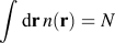 $\int {{\rm{d}}{\bf{r}}n\left( {\bf{r}} \right) = N}$. The first three terms on the right-hand side of Eq. (1) are the noninteracting electron kinetic energy T s[n], the electrostatic repulsion between electrons E H[n], and the energy attributed to the quantum-mechanical exchange and correlation E xc[n] (which includes the difference between the interacting kinetic energy and T s[n]). These terms together comprise the universal functional first identified in the landmark paper by Hohenberg and Kohn,Reference Hohenberg and Kohn7 whose work undergirds the vast enterprise of DFT research. The final term in Eq. (1) describes the interaction between the electrons and the external potential v(r).
For a system composed of atoms, v(r) is generated as a superposition of individual atomic potentials. All-electron calculations employ Coulombic nuclear potentials, while valence-electron-only calculations utilize pseudopotentials that model the combined effect of core electrons and the nuclear charge (the latter combination is referred to as an ion). The total system energy, then, is obtained by adding the appropriate ion–ion interaction energy to Eq. (1). In addition, one can use DFT to determine the forces exerted on individual atoms and the state of stress in a crystal. These properties are computed, in short, by probing the change in system energy induced by infinitesimal displacements of atoms (for forces) or infinitesimal adjustments to the crystal lattice (for stresses).
The usual approach to DFT—and also the particular decomposition of terms given in Eq. (1)—is attributable to Kohn and Sham,Reference Kohn and Sham8 who devised an implicit strategy for computing the exact value of T s[n]. To accomplish this task, KSDFT relies on self-consistently determined one-electron wave functions for a reference system of noninteracting electrons with an electron density that is identical to that of the fully interacting system. Therefore, because the classical electrostatic repulsion term is known explicitly,  ${E_{\rm{H}}}\left[ n \right] = {1 / 2}\int {{\rm{d}}{\bf{r}}} {{\int {{\rm{d}}{\bf{r'}}n\left( {\bf{r}} \right)n\left( {{\bf{r'}}} \right)} } / {\left| {{\bf{r}} - {\bf{r'}}} \right|}}$, only the exchange-correlation energy E xc[n] must be approximated, and this term is expected to be relatively smaller in magnitude than the others. A downside of the one-particle wave function approach is that wave function operations give rise to cubic computational scaling: a doubling of the number of electrons in a simulation tends to increase the computational effort by a factor of eight. This feature of standard KSDFT renders it unappealing, and frequently prohibitive, for simulations involving many hundreds or thousands of atoms. Finally, while KSDFT is not the focus of this article, it is appropriate at this stage to mention the burgeoning field of (quasi-)linear-scaling KSDFT. Although a certain level of maturity has been reached for insulating systems, this topic remains an active area of research.Reference Bowler and Miyazaki12–Reference Aarons, Sarwar, Thompsett and Skylaris14
In OFDFT, T s[n] is computed directly from the electron density rather than indirectly from single-particle wave functions. This original formulation bypasses wave functions entirely, and the simplification in formalism enables DFT simulations with (quasi-)linear computational scaling and a small prefactor. However, an approximation is required because, as with the case of E xc[n], no exact, easily evaluated form for T s[n] is known. (Importantly, OFDFT formulated in this way makes use of the same exchange-correlation functionals that have propelled KSDFT to prominence.) In the following subsection, we introduce a series of approximations for T s[n] that have been applied in materials science research. Subsequently, because many OFDFT studies utilize pseudopotentials to reduce computational expense, we describe the theory of local pseudopotentials (LPSs). Finally, in the concluding subsection, we discuss computational strategies and algorithmic best practices that enable efficient OFDFT calculations.
A. Kinetic energy density functionals
The discussion on kinetic energy density functionals (KEDFs) is divided into three parts. First, we present three relatively simple approximations for T s[n], each of which yields the exact result for a certain special case, and then use these examples to develop a preliminary understanding of the philosophy that underlies the nonlocal functionals used in most of the application work described later. Second, we describe two paradigms that began to emerge during the period between 1985 and 2000. Most of the OFDFT studies chronicled in the latter half of this article rely on approximations for T s[n] that fall within these two categories. Finally, we discuss a series of more recent attempts to improve on the performance of earlier nonlocal functionals.
This treatment is not intended to be a comprehensive review of the full canon of KEDFs. Instead, we emphasize the subset of predominantly nonlocal functionals that provide near-KSDFT accuracy for a limited portion of the periodic table; these functionals enabled most of the research on solid and liquid materials described subsequently. Interested readers will find more information in several review articles that cover KEDFs more broadlyReference Wang, Carter and Schwartz1,Reference Dreizler and Gross6,Reference Ludena and Karasiev15,Reference García-Aldea, Alvarellos and Roy16 and, in addition, we provide an extremely brief discussion on recent advances in single-point KEDF development later in Sec. IV.
1. Three simple approximations for T s[n]
a. Single-orbital systems and the von Weizsäcker functional
For a single, isolated electron in a static external potential, one can infer a ground-state wave function by computing the square root of the ground-state electron density, and thereby obtain from elementary quantum mechanics the exact T s[n] for this simple system. The result was first published by von WeizsäckerReference von Weizsäcker17 (vW) in 1935 and may be written as
 $${T_{{\rm{vW}}}}\left[ n \right] = - {1 \over 2}\int {{\rm{d}}{\bf{r}}{n^{1{\rm{/}}2}}\left( {\bf{r}} \right){\nabla ^2}{n^{1{\rm{/}}2}}\left( {\bf{r}} \right)} = {1 \over 2}\int {{\rm{d}}{\bf{r}}\nabla {n^{1{\rm{/}}2}}\left( {\bf{r}} \right) \cdot \nabla {n^{1{\rm{/}}2}}\left( {\bf{r}} \right)} \quad .$$
The vW functional also provides the exact non-interacting kinetic energy for other single-orbital systems in their ground state, such as two spin-unpolarized electrons or any number of bosons. When applied to systems of many fermions, T vW[n] returns a rigorous lower bound to the full T s[n] and therefore the following expression is general: T s[n] ≥ T vW[n]. The two forms of T vW[n] given in Eq. (2) are related by the divergence theorem and they are equivalent for isolated systems and for systems described with periodic boundary conditions.
b. The free-electron gas and the Thomas–Fermi functional
The free-electron gas is so-named because its members traverse freely across a perfectly flat potential landscape, encumbered only by the Pauli Exclusion Principle. It is generally regarded as the simplest many-fermion system, and its electron density and other properties are constant throughout space; that is, n(r) → n 0. The relationship between the kinetic energy (per unit volume) and the electron density is given by  ${t_0} = {c_0}n_0^{5{\rm{/}}3}$, where c 0 = (3/10) (3π2)2/3 is the appropriate constant for spin-unpolarized electrons.
For more general systems with slowly varying electron densities, a reasonable approximation to the kinetic energy is obtained if one applies the free-electron-gas expression locally, and integrates. This functional,
 $${T_{{\rm{TF}}}}\left[ n \right] = {c_0}\int {{\rm{d}}{\bf{r}}{n^{5{\rm{/}}3}}\left( {\bf{r}} \right)} \quad ,$$
was proposed independently by ThomasReference Thomas18 and FermiReference Fermi19 (TF) in 1927 and it represents the earliest approximation for T s[n] from a historical perspective. Because T TF[n] encodes the Pauli Exclusion Principle, it may also serve as a crude approximation to the excess kinetic energy not accounted for by T vW[n]. The combination T vW[n] + T TF[n] remains exact for a uniform electron gas but introduces error for any single-orbital system.
c. Weakly perturbed free-electron gas
When n(r) deviates only modestly from uniformity—more precisely, when n(r) = n 0 + Δ(r) with |Δ(r)| ≪ n 0 and 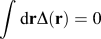 $\int {{\rm{d}}{\bf{r}}\Delta \left( {\bf{r}} \right) = 0}$—the kinetic energy T s[n] may be obtained with high accuracy from the second-order perturbation expansion for a free-electron gas
 $${T_2}\left[ n \right] = {T_{{\rm{TF}}}}\left[ {{n_0}} \right] + {1 \over 2}\int {{\rm{d}}{\bf{r}}} \int {{\rm{d}}{\bf{r'}}\Delta \left( {\bf{r}} \right)} {\left. {{{{\delta ^2}T_{{\rm{s}}}} \over {\delta n\left( {\bf{r}} \right)\delta n\left( {{\bf{r'}}} \right)}}} \right|_{{n_0}}}\Delta \left( {{\bf{r'}}} \right)\quad .$$
The second functional derivative in Eq. (4) is known exactly and is closely associated with the LindhardReference Lindhard20 density–density response function, χ0(k). The exact relationship is given by
 $$F\left[ {{{\left. {{{{\delta ^2}T_{{\rm{s}}}} \over {\delta n\left( {\bf{r}} \right)\delta n\left( {{\bf{r'}}} \right)}}} \right|}_{{n_0}}}} \right] = - {1 \over {{\chi _0}\left( {\bf{k}} \right)}}\quad ,$$
where F[·] indicates a Fourier transform. For spin-unpolarized electrons, χ0(k) has the analytical form χ0(k) = −(k 0/π2)f(k/2k 0), where k = |k|, k 0 = (3π2n 0)1/3, and
 $$f\left( x \right) = {1 \over 2} + {{1 - {x^2}} \over {4x}}\ln \left| {{{1 + x} \over {1 - x}}} \right|\quad .$$
d. Combining the three approximations
Each of these elementary approximations for T s[n] is exact in a certain limit and becomes accurate as an electron density approaches that limit. Consider now the composite functional that one would obtain by starting with T 2[n]—which is correct to second order for a perturbed free-electron gas—and then adding estimated contributions for the third and higher order terms using corrections derived from, say, T vW[n] + T TF[n]. Such a functional would remain accurate for a weakly perturbed electron gas but would potentially be more accurate than T 2[n] by itself for other systems. In fact, this functional, considered by Perrot,Reference Perrot21 is emblematic of a category of functionals initiated by Wang and Teter,Reference Wang and Teter22 which is one of the two categories discussed in the following subsection.
2. Nonlocal functionals based on the Lindhard response function
Most of the materials science studies described in this review were enabled by two classes of approximations for T s[n] that both incorporate the Lindhard response function, χ0(k). The connection between T s[n] and χ0(r)—namely, Eq. (5)—was apparent even during the earliest stages of DFT research.Reference Hohenberg and Kohn7 The functionals described in this section all satisfy Eq. (5) by construction and, as a result, are able to predict expected quantum-mechanical features such as shell structure in atoms and Friedel oscillations in metals. Moreover, a sizable subset of these functionals may be evaluated with (quasi-)linear-scaling computational effort.
a. The Chacón–Alvarellos–Tarazona functional and generalizations
The Chacón–Alvarellos–Tarazona (CAT) functionalReference Chacón, Alvarellos and Tarazona23 was introduced in 1985, and its key ingredient has the form
 $$T_{{\rm{CAT}}}^{{\rm{nl}}}\left[ n \right] = {c_0}\int {{\rm{d}}{\bf{r}}n\left( {\bf{r}} \right){{\bar{n}}^{2{\rm{/}}3}}\left( {\bf{r}} \right)} \quad ,$$
in which  $\bar{n}\left( {\bf{r}} \right)$ refers to a yet unspecified average density, where the averaging procedure probes the fluctuations in n(r) near the point r. The expression in Eq. (7) clearly resembles the TF functional—and it is identical to T TF[n] for the limiting case of a free-electron gas—but it also incorporates the extra, nonlocal information that is encoded in
 $\bar{n}\left( {\bf{r}} \right)$. In the original CAT functional,
 $\bar{n}\left( {\bf{r}} \right)$ is obtained from a spherical average
 $\bar{n}\left( {\bf{r}} \right) = \int {{\rm{d}}{\bf{r'}}w\left( {{k_0}\left( {\bf{r}} \right),\left| {{\bf{r}} - {\bf{r'}}} \right|} \right)n\left( {{\bf{r'}}} \right)}$, where k 0(r) is the local Fermi wave vector, k 0(r) = (3π2n(r))1/3. The weight function w(k 0(r), |r − r′|) is chosen such that the overall functional satisfies Eq. (5), thereby ensuring that it returns the correct result for a weakly perturbed electron gas.
Over time, a variety of modifications to the CAT functional have appeared;Reference García-Aldea, Alvarellos and Roy16,Reference García-González, Alvarellos and Chacón24–Reference González, González, López and Stott29 however, the original spirit is preserved in each case cited. One prominent generalization involves the introduction of a symmetrized, two-point Fermi wave vector,  ${k_0}\left( {\bf{r}} \right) \to k_0^\gamma \left( {{\bf{r}},{\bf{r'}}} \right)$, which transforms the spherical average used initially to obtain
 $\bar{n}\left( {\bf{r}} \right)$ into a nonspherical average to better incorporate nonlocal effects.Reference García-González, Alvarellos and Chacón25 Another more recent modification attempts to improve the accuracy of CAT-like functionals for localized systems.Reference García-Aldea and Alvarellos27 Finally, while the most natural implementations of the CAT functional incurs quadratic computational scaling, several simplifications that are appropriate for extended systems may be evaluated with (quasi-)linear scaling.Reference García-Aldea, Alvarellos and Roy16,Reference García-Aldea and Alvarellos27–Reference González, González, López and Stott29
b. The Wang–Teter, Perrot, Smargiassi–Madden, and Wang–Govind–Carter functionals
A second category of nonlocal approximations for T s[n] is composed of contributions from a variety of authors, each published between 1992 and 1999. The earliest was put forth by Wang and TeterReference Wang and Teter22 and may be written as
 $${T_{{\rm{WT}}}}\left[ n \right] = {T_{{\rm{vW}}}}\left[ n \right] + {T_{{\rm{TF}}}}\left[ n \right] + \int {{\rm{d}}{\bf{r}}} \int {{\rm{d}}{\bf{r'}}{n^{5{\rm{/}}6}}\left( {\bf{r}} \right)w\left( {{k_0},\left| {{\bf{r}} - {\bf{r'}}} \right|} \right){n^{5/6}}\left( {{\bf{r'}}} \right)} \quad .$$
In Eq. (8), k 0 refers to the Fermi-wave vector associated with a fixed reference density n 0, and the integral kernel w(k 0, |r − r′|) is determined from the requirement that the overall functional must satisfy Eq. (5). The modifications proposed by Perrot,Reference Perrot21 Smargiassi and Madden,Reference Smargiassi and Madden30 and Wang et al.,Reference Wang, Govind and Carter31 are similar to Eq. (8) in spirit and differ from Eq. (8) only in the explicitly nonlocal third term. One potential point of concern for functionals of this type comes from an upper bound for T s[n] first conjectured by Lieb:Reference Lieb and Osterwalder32 T s[n] ≤ T vW[n] + T TF[n]. If the third term in Eq. (8) evaluates to a positive number, the bound is violated. Like T WT[n], each of these functionals depends on a fixed reference density, which is usually chosen to be the average density of the system. For this reason, the functionals in this category are most applicable for extended systems and their respective nonlocal terms may be evaluated with (quasi-)linear-scaling computational effort. However, if applied to systems with strongly varying electron densities, these functionals may become variationally unstable.Reference Blanc and Cancès33 Finally, Wang and Teter,Reference Wang and Teter22 as well as Foley and Madden,Reference Foley and Madden34 developed generalizations of the same basic approach that return the exact result up to an additional order in perturbation theory for a weakly varying free-electron gas.
A more significant modification was proposed by Wang, Govind, and Carter (WGC).Reference Wang, Govind and Carter35 The WGC functional is given by
 $${T_{{\rm{WGC}}}}\left[ n \right] = {T_{{\rm{vW}}}}\left[ n \right] + {T_{{\rm{TF}}}}\left[ n \right] + \int {{\rm{d}}{\bf{r}}} \int {{\rm{d}}{\bf{r'}}{n^\alpha }\left( {\bf{r}} \right)w\left( {k_0^\gamma \left( {{\bf{r}},{\bf{r'}}} \right),\left| {{\bf{r}} - {\bf{r'}}} \right|} \right){n^\beta }\left( {\bf{r}} \right)} \quad ,$$
where {α, β} = {5/6 ±  ${\sqrt{5}}$/6} and, importantly, k 0 is replaced with the two-point Fermi-wave vector
 $k_0^\gamma \left( {{\bf{r}},{\bf{r'}}} \right)$ that injects additional density dependence into the nonlocal term. This change is intended to improve the treatment of systems with more rapidly varying densities but does complicate the implementation of the functional. To regain quasi-linear scaling, WGC developed an approximate implementation of their nonlocal term that relies on a Taylor expansion about a fixed reference density. Subsequent work examined the WGC integral kernel in more detailReference Ho, Lignères and Carter36 and also attempted to improve the performance of the WGC functional for nonmetallic systems.Reference Zhou, Ligneres and Carter37
3. Additional nonlocal kinetic energy density functionals
a. Nonlocal functionals for the kinetic potential
The term kinetic potential refers to the functional derivative of the KEDF,  ${v_{{T_{\rm{s}}}}}\left( {\bf{r}} \right) = {{\delta {T_{\rm{s}}}\left[ n \right]} / {\delta n\left( {\bf{r}} \right)}}$. There is some evidence for the contention that
 ${v_{{T_{\rm{s}}}}}\left( {\bf{r}} \right)$ is less severely nonlocal as a functional of the electron density than T s[n], and therefore more amenable to approximation. Moreover, for a given
 ${v_{{T_{\rm{s}}}}}\left( {\bf{r}} \right)$, there exist a variety of integration techniques for regaining the full kinetic energy. Motivated by these considerations, Chai and WeeksReference Chai and Weeks38,Reference Chai and Weeks39 developed a series of functionals for the kinetic potential, including two nonlocal functionals that are similar in spirit to those discussed in the previous section. Chai and Weeks initially tested their nonlocal functionals for atoms and ions. Later, in conjunction with coauthors,Reference Chai, Lignères, Ho, Carter and Weeks40 they applied (quasi-)linear-scaling versions of their functionals to solid-state systems, obtaining very good results for Al and medium-quality results for Si.
b. The Huang–Carter functional
Electrons in a metal may conceivably be excited into states with energies infinitesimally higher than the Fermi level, whereas electrons in insulators must surmount a finite energy gap to access higher-energy states. This fact fundamentally alters the character of the density–density response function for insulators. The Lindhard response function discussed above, χ0(k), has the limiting behavior of a metal. In view of these observations, Huang and Carter (HC) developed a KEDF that incorporates the expected limiting form of the response function for insulators.Reference Huang and Carter41 Specifically, HC devised a modified version of the Wang–Teter functionalReference Wang and Teter22 to increase its applicability for gapped materials. These modifications increase the computational prefactor for the HC functional by one or two orders of magnitude over the Wang–Teter and WGC functionals. The resulting KEDF requires specification of two adjustable parameters; however, by comparing OFDFT results with KSDFT data, HC determined a single pair of values for these parameters for computing the bulk properties of a range of tetrahedrally bonded semiconductors. Subsequent work explored the feasibility of studying molecules with the HC functional.Reference Xia, Huang, Shin and Carter42
c. Nonlocal functionals based on density decomposition
This subsection introduces a strategy for improving the calculation of T s[n] when n(r) has localized features arising from, for example, covalent bonds or d electrons in transition metals. Each of the relevant studies employs a density decomposition of the form n(r) = n del(r) + n loc(r), where n del(r) and n loc(r) refer to, respectively, delocalized and localized contributions to the total electron density. The density—decomposition technique involves (re-)writing T s[n] as
 $${T_{\rm{s}}}\left[ n \right] = {T_{\rm{s}}}\left[ {{n_{{\rm{del}}}}} \right] + {T_{\rm{s}}}\left[ {{n_{{\rm{loc}}}}} \right] + \left( {{T_{\rm{s}}}\left[ n \right] - {T_{\rm{s}}}\left[ {{n_{{\rm{del}}}}} \right] - {T_{\rm{s}}}\left[ {{n_{{\rm{loc}}}}} \right]} \right)\quad ,$$
where the term in parentheses represents an interaction energy that is frequently referred to as the nonadditive kinetic energy.Reference Wesolowski and Warshel43 The nonlocal functionals discussed above are appropriate for computing T s[n del] but less satisfactory for terms involving the localized density. Finally, it is clear from Eq. (10) that the density decomposition philosophy shares much in common with various embedding theories.Reference Wesolowski and Warshel43–Reference Govind, Wang and Carter46
The first attempt at density-decomposition-based OFDFT was made by Huang and Carter,Reference Huang and Carter47 who used the HC functionalReference Huang and Carter41 for T s[n del]; subsequent work by Xia and CarterReference Xia and Carter48,Reference Xia and Carter49 used the WGC functionalReference Wang, Govind and Carter35 for T s[n del], in part to improve computational efficiency. In all cases, simpler functionals of the form aT TF[n] + bT vW[n] were used for terms involving the localized density, in the absence of better choices. In addition, Huang and Carter took the simplifying step of fixing n loc(r) after making an initial decomposition based on the character of n(r) for a single atom. Xia and Carter generalized this approach by allowing n loc(r) to vary self consistently over the course of a calculation, employing a simple probe to assess the degree of localization at any given point. The initial Xia-Carter strategy required an external self consistency loop,Reference Xia and Carter48 while a more recent version does not.Reference Xia and Carter49
d. The enhanced-vW functional
As discussed above, the vW functional returns the exact kinetic energy for single-orbital systems. For this reason, it is reasonable to expect that T vW[n] will play an especially important role in the analysis of more general systems with localized electrons—especially when the localized features are dominated by a single orbital. This observation motivates the enhanced-vW (EvW) functional proposed by Shin and Carter,Reference Shin and Carter50 which is based on the earlier WGC functionalReference Wang, Govind and Carter35 and retains the computational efficiency of the latter. The EvW functional assesses the degree of localization present in an electron density and, when n(r) is dominated by localized features, enhances the relative contribution of the vW term within the overall WGC functional. Specifically, the EvW functional has the following structure
 $${T_{{\rm{EvW}}}}\left[ n \right] = \left( {1 + A} \right){T_{{\rm{vW}}}}\left[ n \right] + \left( {1 - {A \over 2}} \right)\left( {{T_{{\rm{TF}}}}\left[ n \right] + T_{{\rm{WGC}}}^{{\rm{nl}}}\left[ n \right]} \right)\quad ,$$
where  $T_{{\rm{WGC}}}^{{\rm{nl}}}\left[ n \right]$ refers to the nonlocal term from the WGC functional. The enhancement factor A is given the simple form
 $$A = k{\left( {{{{n_{\max }} - {n_{{\rm{avg}}}}} \over {{n_{{\rm{avg}}}}}}} \right)^2}\quad ,$$
where k is an adjustable, material-dependent parameter, and n max and n avg refer to, respectively, characteristic maximum and average densities for the system under study. The strategy for choosing n max and n avg is somewhat subtle but is described in the original paper. This overall philosophy, along with suitable choices for the parameter k, allows EvW to achieve reasonable agreement with KSDFT for III–V semiconductors and to properly describe both the metallic and semiconducting bulk phases of Si.
B. Local pseudopotentials
While all-electron OFDFT rests on a solid theoretical foundation, it is generally not the most expeditious choice from a computational perspective. In practice, a great majority of OFDFT calculations are conducted with the valence electron density alone, and rely on LPSs to represent the combined effect of core electrons and the nuclear potential. Common KSDFT techniques, such as nonlocal pseudopotentials (NLPSs) or the projector-augmented-waveReference Blöchl51 (PAW) approach, are inapplicable because the standard OFDFT lacks orbital information (although we refer the reader to Sec. IV for more discussion on this point).
Over time, the construction of LPSs has evolved in complexity and accuracy. Early OFDFT studies used LPSs with simple analytic forms that were parameterized based on data from experiments or from more accurate electronic structure calculations.Reference Wang and Teter22,Reference Pearson, Smargiassi and Madden52 While this approach is marked by concerns regarding transferability, it remains in use today, sometimes with great success.Reference Shin and Carter53,Reference Legrain and Manzhos54 In principle, LPSs obtained from first principles are applicable in a much wider range of environments, and several protocols have appeared in the literature. Each of the methods for constructing first-principles LPSs has the same goal—to match the electron density (or other properties) obtained with an LPS calculation to that of a KSDFT-NLPS/PAW benchmark—but the methods differ in the choice of reference environment.
1. Atomic local pseudopotentials
Atomic LPSs are based on the KSDFT valence electron density for free atoms and have been successfully applied to the group IV elements Si, Ge, and Sn.Reference Wang and Stott55 However, even when used in KSDFT calculations, atomic LPS results can be insufficiently accurate for the calculation of atomic excitation energies, as well as the band structures of solids. A major drawback is a lack of transferability and insufficient accuracy for crystal applications.Reference Zhou, Alexander Wang and Carter56 Finally, Mi et al. recently proposed a related strategy that develops LPSs directly from first principles norm-conserving pseudopotentials.Reference Zhou, Alexander Wang and Carter56
2. Bulk-derived local pseudopotentials
Bulk-derived LPSs (BLPSs) are based on KSDFT valence electron densities derived from one or more bulk crystalline environments. The first BLPSs were obtained by requiring that an OFDFT calculation (performed with a particular KEDF) reproduces exactly a reference density from a KSDFT calculation; as a result, these BLPSs were KEDF dependent.Reference Watson, Jesson, Carter and Madden57 More recent work has emphasized KEDF-independent BLPSs, which are constructed from KSDFT calculations alone and are therefore expected to be more transferable.Reference Zhou, Alexander Wang and Carter56,Reference Zhou and Carter58,Reference Huang and Carter59 BLPSs have been successfully applied to numerous solid-state calculations on a variety of materials,Reference Xia, Huang, Shin and Carter42,Reference Zhou, Alexander Wang and Carter56,Reference Huang and Carter59 including Li, Mg, Al, Ga, In, P, As, Sb, and Si, as well as the III–V semiconductorsReference Huang and Carter41,Reference Xia and Carter48,Reference Shin and Carter50 GaP, GaAs, GaSb, InP, InAs, and InSb. Additionally, liquid Li and the Li melting temperature have been successfully investigated with a BLPS.Reference Chen, Hung, Huang, Xia and Carter60,Reference Chen, Vella, Panagiotopoulos, Debenedetti, Stillinger and Carter61 However, inaccuracies arise for liquid phases of more complex systems.
3. Neutral pseudoatom method
The neutral pseudoatom (NPA) method was first introduced by ZimanReference Ziman62 in 1964 and later developed by DagensReference Dagens63 for the study of metallic Li and Na. It is based on a representation of the valence-electron density of an atom in a positive background of a uniform electron gas. Anta and MaddenReference Anta and Madden64 used this reference system to develop KEDF-dependent ab initio LPSs, and such LPSs have proven useful for OFDFT studies of liquid metals.Reference González, González and López65 However, because the NPA is constructed from the discrete environment of an isolated atom, inaccuracies can appear for liquids, where the atom is surrounded by others in a disordered array. One successful modification that involves a force-matching procedure was introduced by del Rio and González.Reference del Rio and González66 In this procedure, the initial NPA LPS is modified by the addition of Gaussian functions to minimize the difference in the forces calculated with a NLPS-KSDFT calculation and the NPA LPS-OFDFT calculation for a given liquid configuration. The liquid sample used for the NLPS-KSDFT benchmark calculation must be small (∼100 atoms) and simulated for a short time (∼10 ps). The force-matching modification has been applied successfully to the study of Be, Ca, and Ba.
4. Globally-optimized local pseudopotentials
Recently introduced by three of the authors,Reference del Rio, Dieterich and Carter67 the globally-optimized LPS (goLPS) method is the first construction procedure explicitly designed to represent both solid and liquid phases correctly, and therefore will be especially useful for multi-phase simulations. The goLPS strategy can also be used to improve a given solid or liquid LPS and, thus far, goLPSs have been constructed successfully for Li, Ca, and Ga.
C. Algorithms and implementation details
Several OFDFT codes have been described in detail in the literature.Reference Watson and Carter68–Reference Mi, Shao, Su, Zhou, Zhang, Li, Wang, Zhang, Miao, Wang and Ma75 In this section, we seek to answer the following questions: (i) what capabilities and level of performance can a researcher expect from an OFDFT code; (ii) how have the major algorithmic hurdles been overcome thus far; and (iii) what future algorithmic challenges require attention? The objective and capabilities of OFDFT are very similar to those of KSDFT: both theories endeavor to find, for a given arrangement of atoms and boundary conditions, the ground-state energy and the self-consistent solution for the electron density. While there are technical differences between OFDFT and KSDFT implementations—and, in fact, within the two paradigms separately—the actual computation of static and dynamic properties is typically conducted in a similar fashion. Physical properties are computed from, say, converged electron densities or perhaps extracted from repeated simulations of the same system, each with a slightly modified arrangement of atoms. Because OFDFT codes can be made to scale with (quasi-)linear computational complexity as additional atoms are included in a simulation,Reference Watson and Carter68,Reference Lignères, Carter and Yip76 they are especially appealing for study of phenomena involving large numbers of atoms and/or long time scales. In what follows, we first establish what is required to achieve (quasi-)linear scaling for a single iteration of a self-consistency cycle. Subsequently, we discuss the reduction of absolute evaluation times.
The most basic feature that differentiates OFDFT implementations is the choice of basis set for representing the electron density. Planewave representations (or, almost equivalently, Cartesian grids in real space with equidistant spacing) have been used traditionally in conjunction with judicious use of Fast Fourier Transforms (FFT)s.Reference Watson and Carter68–Reference Chen, Xia, Huang, Dieterich, Hung, Shin and Carter71,Reference Hung and Carter77 Specifically, FFT-assisted convolutions are useful for evaluating many nonlocal KEDF terms, reducing the quadratic scaling of naïve implementations to quasi-linear scaling. Similarly, the electron–electron repulsion energy E H[n] may be obtained almost trivially with a pair of FFTs. The local density approximation for the exchange-correlation term, E xc[n] is straightforward to evaluate without FFTs, and the extra gradient information required by generalized gradient approximations for E xc[n] may also be computed with efficient, FFT-assisted techniques. More care is required for the electron-ion and ion–ion terms, which scale quadratically in naïve implementations. For the ion–ion term, an Ewald summation is frequently required; our code, PROFESS,Reference Ho, Lignères and Carter69–Reference Chen, Xia, Huang, Dieterich, Hung, Shin and Carter71 achieves quasi-linear scaling with a cardinal B-spline implementationReference Essmann, Perera, Berkowitz, Darden, Lee and Pedersen78 of the particle mesh Ewald method. The ion—electron term may also be evaluated with quasi-linear scaling using a B-spline approach for computing the structure factor.Reference Hung and Carter77,Reference Choly and Kaxiras79
FFT-based implementations are known to exhibit limited parallel scalability with standard FFT libraries.Reference Gupta and Kumar80 Because FFTs incur the majority of the communications overhead in an FFT-based OFDFT code—by contrast, integrations over the full grid are nondemanding and occur less often—FFT scalability determines the overall scalability of such codes. However, for many systems of interest, the absolute speed of FFT-based implementations is sufficient even with a limited number of processors; FFTs become a bottleneck only for extremely large systems also requiring very fast (and hence massively parallel) evaluations. A recent demonstration of petascaling OFDFTReference Chen, Jiang, Zhuang, Wang and Carter81 overcomes parallelization limitations by partitioning energy functionals into short- and long-ranged contributions and then employing a multi-grid approach where smooth contributions are evaluated on a coarse global grid while more rapidly varying contributions are evaluated with local “small-box” FFTs. Such techniques can be used for the explicit quantum-mechanical study of millions of atoms. Another approach that is applicable for simulations of medium to large systems (presently, up to tens of thousands of atoms) is to make use of compute accelerators such as GPUs. Even though FFTs are a task not ideally suited for GPUs and hence currently unable to extract even close to theoretical peak performance out of GPU hardware, we find the absolute performance of accelerated KEDF implementations to be excellent.Reference Dieterich, Witt and Carter82 Currently, constraints for GPU-accelerated OFDFT arise because of memory limitations on the accelerators; these limitations begin to appear in the realm of hundreds of grid points per Cartesian dimension.
Purely real-space representations of the electron density, in contrast with FFT-based implementations, trade a small complexity prefactor and code simplicity for better fundamental parallel scalability. Large improvements have been made in recent years to reduce the high prefactor of real-space implementatons.Reference Mi, Shao, Su, Zhou, Zhang, Li, Wang, Zhang, Miao, Wang and Ma75,Reference Gavini, Knap, Bhattacharya and Ortiz83–Reference Motamarri, Iyer, Knap and Gavini85 An important first step is to develop an evaluation strategy for nonlocal terms that does not depend on operations in the reciprocal space. In particular, long-range electrostatic interactions, including Poisson terms,Reference Motamarri, Iyer, Knap and Gavini85 can be computed from a local variational problem. Similarly, the nonlocal integral kernels appearing in the WGC KEDF can be reformulated as a series of Helmholtz equations in real space.Reference Choly and Kaxiras86 Results discussed in the literature show that such real-space algorithms can be used to simulate tens of thousands of atoms with full atomic resolution, and millions using coarse-graining techniques.Reference Gavini, Bhattacharya and Ortiz87
Next, we note one important implementation detail pertaining to the use of preconditioners and electron density optimization approaches in OFDFT. The computational prefactor for OFDFT calculations depends on the number of iterations required to obtain a converged total energy and electron density. Some insight has been gained on preconditioning strategies for bulk systems;Reference Hung, Huang and Carter88 however, possibilities for development remain, particularly regarding transferable preconditioners and local optimization procedures applicable to finite systems.
While we emphasize OFDFT in this review, other algorithmic ingredients such as techniques for geometry optimization and MD propagators are shared with KSDFT approaches. The typical performance of OFDFT codes allows one to study systems with dynamic exploration methods such as MD and also makes OFDFT an attractive ingredient for multi-scale and quasi-continuum simulations.Reference Fago, Hayes, Carter and Ortiz89–Reference Radhakrishnan, Gavini, Wesolowski and Wang91 Future integration of OFDFT with techniques beyond these, such as advanced sampling and exploration techniques, will be straightforward and should prove to be scientifically beneficial.
III. MATERIALS RESEARCH WITH OFDFT
This section reviews contributions of OFDFT to the understanding of a diverse range of materials, including solids, liquids, and multi-phase systems. Each of the studies described below was conducted with OFDFT calculations, sometimes in conjunction with other methods. We eschew discussion of most computational details but provide references for the interested reader. Unfortunately, quantitative agreement between OFDFT and standard KSDFT varies on a case-by-case basis and, for any given material, one must verify that the two theories give the same result for small systems before proceeding to larger systems accessible only with OFDFT. For this reason, the studies that we discuss typically include such a validation step to promote confidence in the results. In general—at least with the nonlocal functionals described above—quantitative agreement between OFDFT and KSDFT (and/or experimental data) is achieved for light metals and their alloys. Useful quantitative results may also be obtained for other materials but, at present, more caution is warranted.
A. Solids
Bulk crystalline solids, particularly those without strongly correlated electrons, were among the earliest successes of both KSDFT and OFDFT.Reference Jones and Gunnarsson92 For simple cases, such as a defect-free solid composed of a single element, simulations involving a few or tens of atoms subject to periodic boundary conditions are sufficient for determining physical properties such as equilibrium volumes, elastic behavior, and relative energies of various crystalline phases—and the computational efficiency of OFDFT is generally unnecessary for such cases. However, analysis of alloy phases (e.g., high entropy alloysReference Miracle and Senkov93) may require hundreds or even thousands of atoms. Moreover, the behavior of real solids is altered by defects and defect-driven phenomena, some of which—such as the nucleation and motion of dislocations, or diffusion along grain boundaries in a polycrystal—may affect thousands of atoms. Finally, other defects involve only a few atoms but occur in tiny concentrations, meaning that many-atom simulations are required for a realistic treatment. The following subsections explore these topics more in detail.
1. Solid alloys
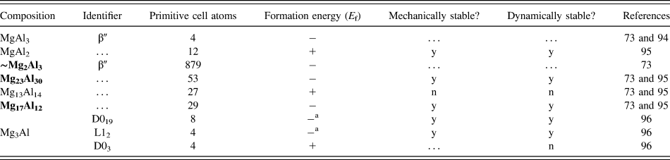
The majority of OFDFT studies on crystalline alloys thus far have considered Mg–Al compounds. Both Al and Mg are abundant metals, and Mg–Al intermetallic compounds have high strength-to-weight ratios and other favorable mechanical properties. Moreover, one expects that OFDFT will be reasonably accurate for Mg–Al compounds of a wide range of compositions because the valence electrons are delocalized in both bulk Al and bulk Mg. Several roles for OFDFT calculations are illustrated below using examples drawn from a series of studies on Mg–Al alloys.Reference Das, Iyer and Gavini73,Reference Carling and Carter94–Reference Zhuang, Chen and Carter96 Perhaps the most important task is to assess the stability (or meta-stability) of a candidate compound, which is a multipart endeavor. A thorough stability analysis involves consideration of a compound’s formation energy, elastic behavior (mechanical stability), and phonon spectra (dynamical stability).
The formation energy, E f, is a useful first descriptor of structural stability: a negative E f provides evidence for stability, whereas a positive E f suggests that the compound is energetically unfavorable and may even decompose into secondary phases. Formation energies at zero Kelvin have been computed for a variety of Mg–Al compounds. Table I summaries the results of some of these calculations. For simplicity, Table I gives only a plus sign if the computed value of E f is positive and a minus sign for negative E fs, reflecting either a consensus in the literature or (in a few cases) the result that is expected to be the most accurate. We note that while most compounds presented in Table I have relatively small unit cells, the β′-Mg2Al3 phase considered by Das, Iyer, and GaviniReference Das, Iyer and Gavini73 requires an 879 atom simulation. The three compounds in Table I listed in boldface type are found in the experimental Mg–Al phase diagram, with β′-Mg2Al3 among them.
Summary of stability analyses performed on a variety of Mg–Al compounds. Those compounds which pass all three stability tests (described in the text) are expected to be at least meta-stable. The compounds listed in boldface type are present in the experimental phase diagram; each of these compounds passes all three stability tests.

a KSDFT calculations and evaluation of the zero point energy were required to resolve ambiguities in the formation energies for these compounds.
The utility of OFDFT becomes more apparent for assessment of mechanical and, especially, dynamical stability. A compound’s mechanical stability is closely related to its elastic behavior, and a mechanically stable compound in its ground state will resist any applied strain. One verifies mechanical stability by ensuring that a compound’s stiffness tensor is positive definite; if not, the compound will be mechanically unstable. These elastic properties are synthesized from many simulations of the same cell, each perturbed by a small strain. Table I indicates those compounds which pass the mechanical stability test, when the data are available.
Dynamical stability is assessed from the crystal’s phonon spectra: imaginary phonon modes, when observed, imply that the compound is dynamically unstable. The simulations that are used to generate phonon spectra require more atoms than are in the simple unit cell; for example, the phonon spectra calculations for Mg23Al30, another compound in the experimental phase diagram, involved simulations of 1431 atoms.Reference Zhuang, Chen and Carter95 Those compounds which pass the dynamical stability test are also reported in Table I. Phonon spectra, once computed, enable determination of thermodynamic properties such as the temperature-dependent formation energy, heat capacity, and thermal expansion coefficient.
A recent study by Zhuang, Chen, and CarterReference Zhuang, Chen and Carter95 illustrates an additional use for OFDFT in the study of alloys: computational discovery of new materials. This study used OFDFT to rapidly screen 101 Mg–Al compounds and used these results in conjunction with a cluster expansion model to explore 5675 additional compounds. After narrowing the field to three compounds, each with composition Mg3Al, Zhuang, Chen, and Carter then used KSDFT calculations to predict a new meta-stable compound (D019 Mg3Al) that is expected to exhibit greater stability and superior ductility when compared with other candidate structures of the same composition.
While the majority of OFDFT studies on solid alloys have considered Al and Mg, there are a growing number of examples involving other materials. For example, Shin and Carter have explored plasticity in BCC Mg–Li alloys.Reference Shin and Carter53 Improvements in KEDFs have also spurred new applications, including studies of crystalline Li–Si alloysReference Xia and Carter97 and amorphous Li–Si alloys.Reference Xia and Carter49
2. Defects in solids
The existence and behavior of defects in a crystalline solid can alter its properties dramatically, and OFDFT enables realistic simulations of such defects that are challenging or impossible to conduct with most other methods. One can employ several distinct strategies for modeling a defect within an extended system. Codes that employ periodic boundary conditions model a periodic array of defects, and the user increases the size of the simulation cell until interactions between the defects become negligible. Bulk Dirichlet boundary conditions are another option, where the boundaries are fixed in accordance with the electronic structure of the bulk material. This choice models a true isolated defect but, again, requires the user to increase the computational domain until the property of interest reaches a converged value.
a. Vacancies and vacancy clusters
A useful starting point is a single, isolated vacancy within a face-centered cubic (FCC) Al lattice. The formation energy E vf of this defect at zero Kelvin has been computed with OFDFT by several authors.Reference Wang, Govind and Carter31,Reference Wang, Govind and Carter35,Reference Das, Iyer and Gavini73,Reference Ho, Ong, Caspersen and Carter98–Reference Qiu, Lu, Ao, Huang, Tang and Chen100 When the defect is modeled with periodic boundary conditions, the value of the formation energy converges for simulations of 108–256 atoms.Reference Das, Iyer and Gavini73,Reference Ho, Ong, Caspersen and Carter98 However, larger simulations of at least 864 atoms are required for convergence of the electronic structure,Reference Das, Iyer and Gavini73 which exhibits meaningful perturbations from its bulk character over distances of at least five lattice units from the defect. In contrast, when the isolated defect is studied with bulk Dirichlet boundary conditions, neither E vf nor the electronic structure converge until the cell size reaches 864 atoms.Reference Das, Iyer and Gavini73 In addition to the vacancy formation energy, Ho et al. also examine the diffusion kinetics of vacancy motion.Reference Ho, Ong, Caspersen and Carter98 Finally, in part because the aggregation of vacancies may lead to larger defects such as voids, several authors have investigated the behavior of vacancy clustersReference Radhakrishnan and Gavini84,Reference Ho, Ong, Caspersen and Carter98,Reference Radhakrishnan and Gavini99 including di-vacancies, tri-vacancies, tetra-vacancies, and one example involving a 19-vacancy cluster.Reference Radhakrishnan and Gavini84
b. Dislocation nucleation, structure, and motion
Dislocations are among the most important many-atom defects because dislocation nucleation, structure, and motion, as well as interactions between dislocations and other defects such as grain boundaries, strongly influence the plastic deformation behavior of metals. In the immediate neighborhood of a dislocation, the electronic structure is disrupted rather severely from its bulk character and so a simulation approach that adheres to the appropriate physics is essential. Away from its core region, a dislocation generates a long-ranged elastic strain field that is also an important part of the overall effect. A simulation tool for dislocations must be able to faithfully capture both phenomena.
The initial series of OFDFT studies in this area examined the onset of plasticity via dislocation nucleation developing at surfaces during nanoindentation.Reference Fago, Hayes, Carter and Ortiz89,Reference Hayes, Fago, Ortiz and Carter101–Reference Peng, Zhang, Huang, Carter and Lu103 (Strictly, the works described in this paragraph were conducted by coupling OFDFT with a local quasi-continuum method,Reference Tadmor, Ortiz and Phillips104–Reference Peng, Zhang, Hung, Carter and Lu106 but we will not elaborate on the distinction here.Reference Ho, Huang and Carter107) The first papers in this seriesReference Fago, Hayes, Carter and Ortiz89,Reference Hayes, Fago, Ortiz and Carter101 used a simulated spherical indenter of 750 nm to probe Al surfaces, highlighting the importance of using indenters with experimentally relevant sizes. Subsequent studies made similar investigations for an Al3Mg alloyReference Hayes, Ho, Ortiz and Carter102 and an Al thin film with Mg impurities.Reference Peng, Zhang, Huang, Carter and Lu103 More force was required to indent the Al3Mg alloy than was required to indent Al, which was an expected result; however, in the Al thin film case, both hardening and softening were observed, depending on the local distribution of Mg impurities.
Multiphysics strategies that couple OFDFT with classical molecular mechanics simulations have also been used for the study of dislocations. Choly et al. applied such an approach to examine the core structure of a screw dislocation in Al.Reference Choly, Lu, E and Kaxiras90 Zhang and Lu, using a similar method, investigated the diffusion of a Si atom along an edge dislocation in Al.Reference Zhang and Lu108
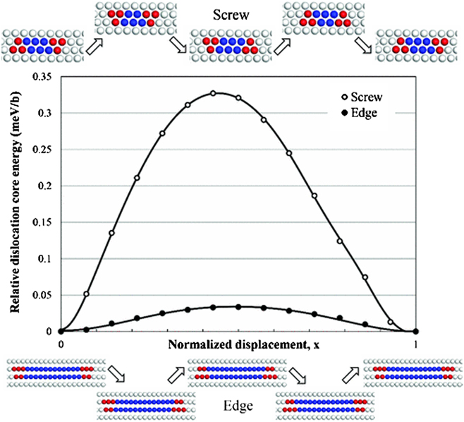
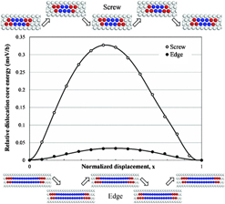
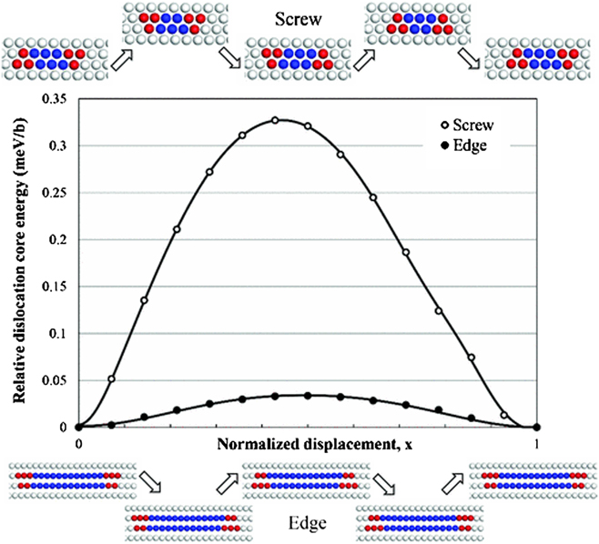
Finally, OFDFT has also enabled direct, atomic-scale study of the structure of edge and screw dislocations in both AlReference Shin, Ramasubramaniam, Huang, Hung and Carter109–Reference Das and Gavini111 and Mg.Reference Shin and Carter112 These simulations generally required at least 1500–3000 atoms, and the authors observed perturbations in the electronic structure that extend for tens of Ångstroms from the main defect, or more. Follow-up studies considered the motion of dislocations in both AlReference Shin and Carter113 and Mg,Reference Shin and Carter114 as well as in Mg–Li alloys.Reference Shin and Carter53 Fig. 1 shows the energy barrier to motion for both edge and screw dislocations in Al. Finally, a recent study examined a possible originating mechanism for dislocations in bulk Al, which involves the collapse of a 19-atom cluster into a dislocation loop.Reference Radhakrishnan and Gavini84
Variation of dislocation core energies for screw and edge dislocations in aluminum as a function of the normalized displacement x traveled by the dislocation core. The energy unit is meV/b where b is the Burgers vector. Insets show corresponding atomic configurations of the screw (upper inset) and the edge (lower inset) dislocation cores along the minimum energy path. Gray, blue, and red spheres indicate atoms locally in face-centered cubic, hexagonal close-packed, and unknown crystal structures, respectively. Reproduced figure with permission from Shin and Carter, Phys. Rev. B 88, 064106 (2013). Copyright 2017 by the American Physical Society.
c. Other large-scale defects
A few OFDFT studies have considered other large-scale defects in solids. For example, Watson and Madden used OFDFT-MD to simulate grain boundary migration in crystalline sodium.Reference Watson and Madden115 Hung and Carter explored ductile crack propagation in Al,Reference Hung and Carter116 contrasting predictions made by OFDFT with predictions made using a classical potential. Finally, a recent study by Chen et al. determined the optimized structure for a polycrystalline Li sample consisting of eight grains, each with a radius of approximately 60 Å, and nearly 400,000 atoms.Reference Chen, Jiang, Zhuang, Wang and Carter81
d. Nanoscale materials
The properties of nanostructured solids can differ dramatically from their bulk counterparts and OFDFT has been used to investigate several categories of nanoscale materials. For example, Watson and Carter considered an array of Al quantum dots,Reference Watson and Carter68 investigating the effect of separation distance on the decay of the electron density in the vacuum region between adjacent quantum dots. A number of studies—see Ref. Reference Aguado, González, González, López, Núñez, Stott, Wesolowski and Yang117 for a summary—have considered alkali metal clusters and alkali metal alloy clusters. OFDFT has also been used to study the mechanical properties of Al nanowires,Reference Ho and Carter118,Reference Hung and Carter119 including elastic properties and mechanisms for tensile yielding. We expect studies of this kind to become increasingly common as OFDFT advances in maturity.
B. Liquids
This section reviews the application of OFDFT-MD to liquid metals and alloys. In principle, OFDFT allows for a realistic treatment of liquids because large samples may be considered for long simulation times. The most success so far has been achieved for simple (s- and p-bonded) metals because these systems may be treated accurately by available KEDFs and LPSs due to their nearly-free-electron-like nature.
1. Bulk liquid metals
Over the last fifteen years, the OFDFT-MD method has been applied to describe a wide range of static, dynamic, and electronic properties of simple liquid metals. The study of time-dependent phenomena usually requires long simulations involving thousands, or tens of thousands, of configurations to avoid problems associated with noise and limited correlation time. OFDFT-MD is well suited for this task, while KSDFT-MD simulations of liquids are usually restricted almost entirely to the study of static properties.
s- and p-bonded liquid metals have been studied extensively with OFDFT, beginning with the pioneering work of Madden and coworkers on the static structure of liquid Na, Mg, and Al.Reference Foley, Smargiassi and Madden120,Reference Anta, Jesson and Madden121 Others considered the single-particle dynamic properties of liquid Li.Reference Chen, Hung, Huang, Xia and Carter60,Reference Anta and Madden64 In addition, OFDFT-MD has been used to study the static and dynamic properties of liquid CsReference Gómez, González, González, Stott, Dalgiç and Silbert28 at several points along the liquid–vapor coexistence line. The first study on collective dynamic properties of liquid alkaline-earth metals occurred in 2009; in this work, a special feature was observed in the static structure factor, S(q), of liquid Mg.Reference Şengül, González and González122 This special feature is a shoulder on the second peak of S(q), which is related to the capacity of the liquid metal to undercool. Subsequent studies on Be, Ca, and BaReference del Rio and González66 revealed the same feature, making it a common property of liquid alkaline-earth metals.
Of the p-bonded liquid metals, Al has been studied most often because of its nearly-free-electron-like nature. Work by González et al.Reference González, González, López and Stott29,Reference González, González, López and Stott123 considered the static and dynamic properties of Al at various temperatures, and warm dense Al was recently studied by White et al.Reference White, Richardson, Crowley, Pattison, Harris and Gregori124 and Sjostrom and Daligault.Reference Sjostrom and Daligault125 White et al. highlighted the inability of classical MD to fully capture quantum effects in cases where electron oscillations couple with ion-acoustic modes, whereas OFDFT includes these effects by continuously updating the electronic response. Sjostrom and Daligault compared OFDFT results to KSDFT results, obtaining excellent agreement for several properties, and were able to use OFDFT to study much higher temperatures than those accessible with KSDFT because the computational cost of their method does not increase with temperature.
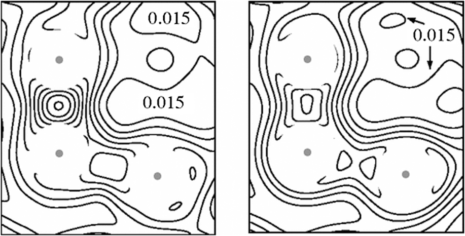
OFDFT-MD studies on complex liquid metals have been performed successfully for liquid GaReference González and González126 and liquid Si under pressure.Reference Delisle, González and Stott127,Reference Delisle, González and Stott128 In both cases, a peculiar shoulder in the main peak of S(q) was observed at several temperatures. In addition, covalent-like bonding present in both liquid Ga and liquid Si was studied with OFDFT; Fig. 2 shows a comparison between OFDFT- and KSDFT-derived density profiles for liquid Ga, and reasonable agreement is apparent.
Electron density for a triplet of Ga atoms at 373 K obtained with OFDFT (left) and KSDFT (right). The contour lines are plotted for values of the density equal to 0.010 electrons/a.u., which corresponds to the minimum inside the peanut-shaped line in the right part of the KSDFT data, and then for increments of 0.005 electrons/a.u. Contour lines within the core radius (≈0.75 Å) of each atom have been deleted because the pseudodensity within the core has no physical meaning. Reproduced figure with permission from González, González, and Stott, Phys. Rev. B 77, 014207 (2008). Copyright 2017 by the American Physical Society.

2. Bulk liquid metal alloys
The field of liquid metal alloys was stimulated by the results of a classical MD simulation of liquid Li4Pb by Jacucci et al.,Reference Jacucci, Ronchetti and Schirmacher129 who observed a new, high-frequency mode supported by the Li atoms only and named it the fast-sound mode. The dispersion curve for pure liquid metals, which contains information about the propagation of collective density fluctuations, has only one branch that begins in the hydrodynamic regime corresponding to very small wave vectors (q) and extends to higher wave vectors. (The slope of the dispersion curve for q → 0 is the adiabatic sound velocity.) In contrast, the dispersion curve for liquid metal alloys has one branch in the hydrodynamic regime and then splits into two branches as the wave vector increases. The two branches correspond to two separate modes, the fast-sound mode and the slow-sound mode, and the bifurcation signals the onset of a dynamic decoupling between the two types of particles. Accordingly, the fast mode is expected to resemble the individual dispersion relation of the corresponding light particle fluid.Reference Campa and Cohen130,Reference Westerhuijs, Montfrooij, de Graaf and de Schepper131 The OFDFT-MD method has been applied to several liquid metal alloys (Na–Cs,Reference Blanco, González, González, López and Stott132 Li–Na,Reference González, González, López and Stott133 and Ga–InReference Aguado, González, González, López, Núñez, Stott, Wesolowski and Yang117) to gain insight into the existence and properties of the collective excitations in these liquids as well as to study the fast-sound mode. Homo-coordinating tendencies are observed for Na–Cs and Li–Na, where each particle tends to be surrounded by particles of the same type, but the segregating tendency lessens as temperature increases.
3. Liquid metal surfaces
The study of the structure of free liquid surfaces has attracted much theoretical and experimental attention, with a strong emphasis on the possible existence of liquid surface layers. It had long been believed that the change in the ion density when crossing from the liquid into the vapor is monotonic.Reference Rowlinson and Widom134 X-ray measurements on several nonmetallic liquidsReference Ocko, Wu, Sirota, Sinha and Deutsch135 revealed density profiles that decay smoothly and monotonically from the high-density bulk liquid to the low-density vapor. However, oscillatory density profiles extending several atomic diameters into the bulk liquid were observed with X-ray measurements of several liquid metals (e.g., GaReference Regan, Kawamoto, Lee, Pershan, Maskil, Deutsch, Magnussen, Ocko and Berman136) and alloys (e.g., In–GaReference Regan, Pershan, Magnussen, Ocko, Deutsch and Berman137). This feature, which suggests a layering parallel to the interface, is of great interest. Given that metallic bonding is very different from that of molecular fluids, it is not surprising that nonmonotonic oscillations in the density are observed for the former in contrast to the latter.
In a metallic system, the nature of the interactions between ions changes drastically across the liquid–vapor interface. The computational demands of the KSDFT-MD method have restricted its application to only two systems, l-Si and l-Na,Reference Fabricius, Artacho, Sánchez-Portal, Ordejón, Drabold and Soler138,Reference Walker, Marzari and Molteni139 but OFDFT-MD has proven capable of treating many more liquid metal and binary alloy surfaces. Work on Li and Na liquid surfaces with OFDFT-MD,Reference González, González and Stott140 for example, clearly revealed the surface layering phenomenon. Subsequently, liquid surfaces of more complex elements (K, Rb, Cs, Mg, Ba, Al, Tl, Si, Ga, and In) were also studied, which led to the verification of a scaling relationship between the wave length of ionic oscillations and the radii of the associated Wigner–Seitz spheres.Reference González, González and Stott141,Reference González and González142 In addition, OFDFT-derived estimates for the reflectivity agreed well with X-ray measurements.Reference Xia and Carter162,Reference Della Sala, Fabiano and Constantin163
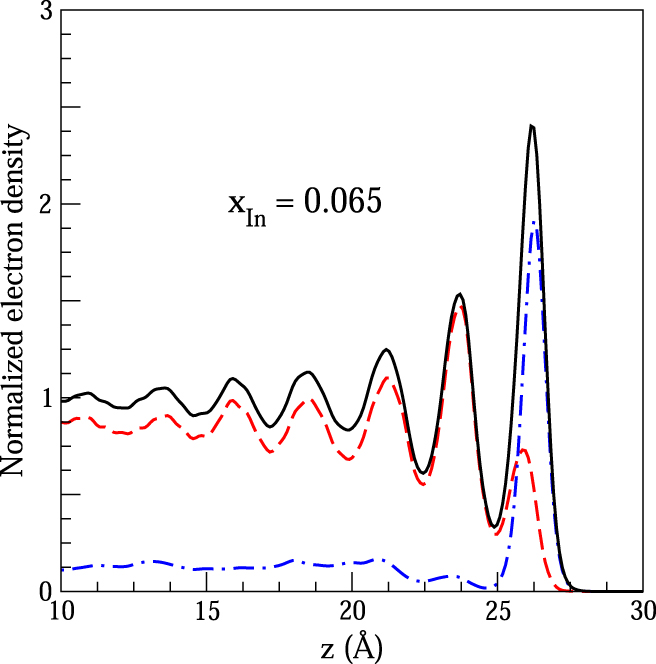
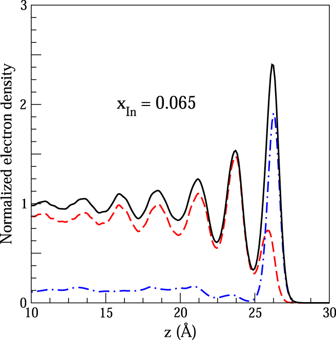
First-principles MD studies of liquid metal alloy surfaces have only been possible with OFDFT-MD. So far, the work has been restricted to the Ga–In alloy at the eutectic pointReference González and González142 and several concentrations of the interalkali alloys Na–K, Na–Cs, and Li–Na.Reference González, González and Stott143,Reference González and González144 An interesting segregation tendency has been observed and attributed to differing surface tensions between the constituents of the alloy; the result is a high concentration at the surface of the compound with the lowest surface tension, as would be expected thermodynamically. This phenomenon is clearly seen in Fig. 3, which shows the density profile for a liquid surface of GaIn, as well as profiles for the individual Ga and In contributions. Specifically, the normalized contribution of In increases dramatically at the surface on the right hand side of Fig. 3.
Total electron density, normalized to the bulk value of the slab, for liquid Ga0.935In0.065 (thick continuous line). The dashed and dash-dotted lines are the Ga and In contributions, respectively, to the total electron density. Received by private communication from the authors of Ref. Reference González and González142, and used with permission.
C. Multi-phase systems
A great number of technological and physical processes, such as soldering, lubrication, and crystal growth or melting, involve more than one phase of matter. Long simulation times are required to model these systems, along with accurate representations of all phases and phase transitions. OFDFT-MD is an alternative to classical MD that provides (in principle) a more accurate description of the system, while retaining manageable computational expense.
1. Solid-liquid interfaces
Early studies of solid–liquid interfaces regarded the solid as a continuous system and modeled its interaction with the liquid using a potential that depended only on the distance from the wall. However, a truly accurate description of interfaces between phases requires an atomic-scale description and, in particular, a proper description of the forces between atoms. We concentrate first on studies related to the static and dynamic properties at solid–liquid interfaces and then comment more extensively on melting temperature calculations in the next subsection.
The solid–liquid interface most studied with OFDFT-MD has been that of Al. The first such simulation was reported in 2000 by Jesson and Madden,Reference Jesson and Madden145 who studied a solid Al surface in equilibrium with liquid Al. However, that study predicted a melting temperature that was much lower than experiment, suggesting deficiencies in the KEDF as well as in the LPS. Later work by González and GonzálezReference González and González146 examined liquid Al at 1000 K in contact with three different orientations of FCC Al: the (100), (110), and (111) surfaces. Interestingly, results differed depending on orientation. While in contact with the (100) surface, only the first layer in the liquid exhibited solid-like ordering, whereas the (111) surface induced a full solidification of the liquid which began to crystallize layer by layer.
In 2013, Aguado et al.Reference Aguado, González, González, López, Núñez, Stott, Wesolowski and Yang117 reported work on a solid–liquid interface between two dissimilar metals: liquid Li on solid Ca at a temperature of 470 K. Their periodic simulation cell contained vacuum, 576 Ca atoms arranged in 16 solid layers, and 2000 Li atoms in the liquid phase. An interesting phenomenon developed in the first liquid layer: the Li atoms in this layer followed one-dimensional trajectories along the channels on the exposed FCC (110) surface of Ca atoms.
2. Solid-liquid phase transitions
The calculation of a material’s melting curve (i.e., how its melting temperature changes with pressure) is an arduous task for which several methods can be used, including the heat-until-melts scheme,Reference Chokappa and Clancy147 the (solid–liquid) coexistence approach,Reference Morris, Wang, Ho and Chan148 and the Z-method.Reference Belonoshko, Skorodumova, Rosengren and Johansson149 The heat-until-melts method is subject to superheating;Reference Chokappa and Clancy147 it therefore yields an upper bound to the true melting temperature (the so-called mechanical melting temperature). OFDFT-MD simulations of the mechanical melting temperature of Li explored the effect of simulation cell size and concluded that at least 256 atoms must be included to achieve property convergence. The coexistence approach provides a more refined estimate of a material’s melting temperature but requires a larger sample to accommodate simultaneous representation of both solid and liquid phases.Reference Chen, Hung, Huang, Xia and Carter60
The light alkali metals Li and Na undergo a series of phase transitions when subjected to compression, and this behavior is reflected in the associated melting line. In both cases, the melting curve reaches a maximum, and thereafter, as pressure is increased, the melting temperature decreases to a minimum before increasing again with a positive slope.Reference Gregoryanz, Lundegaard, McMahon, Guillaume, Nelmes and Mezouar150,Reference Marqués, McMahon, Gregoryanz, Hanfland, Guillaume, Pickard, Ackland and Nelmes151 Only the melting curve of Na has been studiedReference Marqués, González and González152 in this capacity with OFDFT-MD, along with changes in the static, dynamic, and electronic properties of the liquid as pressure is increased. Analysis of the dynamic properties revealed that the increase in density due to pressurization increased the importance of interatomic collisions in controlling the dynamics of the system.
IV. OUTPOSTS ON THE OFDFT FRONTIER
This section contains brief discussions of additional topics that, while less directly connected to the application studies reviewed in the previous section, are nonetheless at the forefront of OFDFT research. The range of topics includes “new approaches to old ideas,”Reference Karasiev, Chakraborty, Trickey, Bach and Delle Site4 as well as rather serious departures from the usual LPS approach.
A. Recent advances in single-point kinetic energy density functionals
Single-point functionals of the electron density have the general form  $F\left[ n \right] = \int {{\rm{d}}{\bf{r}}f\left( {n\left( {\bf{r}} \right),\nabla n\left( {\bf{r}} \right), \ldots } \right)}$, and are evaluated with one, single integral. In contrast, aside from T TF[n] and T vW[n], the KEDFs discussed in Sec. II are two-point, nonlocal functionals; their evaluation requires two integrals. The relative simplicity of single-point functionals makes them advantageous from a computational standpoint. While, historically, single-point approximations for T s[n] have been insufficiently accurate for reliable, self-consistent OFDFT calculations on solids and liquids, progress in this subfield has accelerated recently.
There are at least three scenarios—aside from the self-consistent OFDFT calculations at low temperatures that we have emphasized thus far—in which single-point functionals have flourished. First, at high temperatures, such as those in the warm dense matterReference Graziani, Desjarlais, Redmer and Trickey9 regime straddling condensed matter physics and plasma physics, one typically observes smoothing in sharp quantum features that are present in the T → 0 limit. This phenomenon eases in some ways (and complicates in others) the challenge of determining OF approximations for the noninteracting free energy functional. Second, subsystem DFTReference Jacob and Neugebauer10,Reference Krishtal, Sinha, Genova and Pavanello11 and various embedding approaches employ OF approximations for the non-additive kinetic energy;Reference Wesolowski and Warshel43,Reference Cortona45 fortuitous error cancellation and the smaller magnitude of the nonadditive contribution compared with the full T s[n] can again simplify the task somewhat. Finally, recent advances in the design of exchange-correlation functionals have incorporated the non-interacting kinetic energy density as an ingredient, and OF approximations for this quantity have proven useful.Reference Perdew and Constantin153,Reference Śmiga, Fabiano, Constantin and Della Sala154
Single-point approximations for T s[n] have a long history that, for the sake of brevity, we do not discuss here and instead refer to prior reviews.Reference Wang, Carter and Schwartz1,Reference Karasiev, Chakraborty, Trickey, Bach and Delle Site4,Reference Dreizler and Gross6,Reference Ludena and Karasiev15,Reference García-Aldea, Alvarellos and Roy16,Reference Tran, Wesolowski, Wesolowski and Wang155 Our rather modest aim is simply to direct the reader to a small number of the very latest advances in this category. Generally, single-point density functionals rely on the value of n(r) at each point and a few other dimensionless ingredients such as the reduced gradient |∇n|/(2(3π2)1/3n 4/3) and the reduced Laplacian ∇2n/(4(3π2)2/3n 5/3). Functional developers combine these ingredients based on a variety of overlapping philosophies. Perhaps the most fundamental approach is to posit a functional form that accords with the collection of exact constraints that the true functional has been determined to obey.Reference Perdew and Constantin153,Reference Karasiev, Jones, Trickey and Harris156–Reference Karasiev, Trickey, Sabin and Cabrera-Trujillo158 Investigations that analyze the behavior of local kinetic energy density are useful in this regard.Reference Cancio, Stewart and Kuna159–Reference Finzel164 A related series of studies takes inspiration from the semiclassical limit of atoms as Z → ∞Reference Elliott, Lee, Cangi and Burke165–Reference Cancio and Redd169 and another approach seeks to impose proper representation of atomic shell structure.Reference Finzel170 One can also incorporate exact solutions for simplified model systems such as the locally-linearized potential modelReference Constantin and Ruzsinszky171,Reference Lindmaa, Mattsson and Armiento172 or the jellium-with-gap modelReference Constantin, Fabiano, Śmiga and Della Sala173—or simply search for the best combination of ingredients with a brute force scan.Reference Śmiga, Fabiano, Constantin and Della Sala154 Lastly, we mention an intriguing approach that makes use of a new ingredient, the reduced Hartree potential, although this functional is not strictly a single-point functional.Reference Constantin, Fabiano and Della Sala174
B. Angular-momentum-dependent OFDFT
Angular-momentum-dependent (AMD) OFDFT was conceived by Ke et al.Reference Ke, Libisch, Xia, Wang and Carter175,Reference Ke, Libisch, Xia and Carter176 Recalling that OFDFT regards the electron density, n(r), as the sole quantity to be varied, the primary innovation of AMD-OFDFT is the introduction of single particle density matrices that describe the system in regions of space immediately surrounding each nucleus. This partitioning of the system domain—atom-centered spheres stitched together by an interstitial region—is commonly referred to as a muffin-tin geometry. Outside any particular atom-centered sphere, the AMD-OFDFT approach describes the system with the electron density alone, as is the case for ordinary OFDFT.
In principle, the extra information encoded in the onsite density matrices provides a more complete description of the physical system and therefore should enable more accurate calculation of the system energy. Importantly, one anticipates improvements over regular OFDFT for both kinetic energy and potential energy terms. Improvement for the potential energy is possible because the formalism is no longer restricted to LPSs and may instead treat electrons with different angular momenta differently, as is usually done with KSDFT.
The original articles by Ke et al.Reference Ke, Libisch, Xia, Wang and Carter175,Reference Ke, Libisch, Xia and Carter176 demonstrated the validity of such an approach by showing that it could be used to compute bulk properties of the transition metal Ti. The localized d electrons in these materials typically preclude any successful application of OFDFT. However, this proof-of-principle work utilized a parameter fitting step that simplifies the overall formalism but reduces transferability. Efforts to overcome these limitations are ongoing.
C. OFDFT implementation with the PAW method
The final exampleReference Lehtomäki, Makkonen, Caro, Harju and Lopez-Acevedo74 harnesses the PAW method,Reference Blöchl51 which is well-established for KSDFT, in an OFDFT context. Applying the oft-used technique of interpreting the square root of the electron density as a pseudo-orbital, the authors reformulate the OFDFT problem so that it can be described by an effective Schrödinger equation for a model system. From there, they employ the PAW decomposition to conduct efficient all-electron, frozen-core calculations with OFDFT. When the same semi-local OFDFT functionals are used in both cases, the authors demonstrate their method agrees well with results obtained from more expensive, explicitly all-electron simulations. However, agreement with KSDFT is less satisfactory unless a parameter fitting step is used. Unfortunately, it is not immediately clear how to combine this general approach with the more accurate, nonlocal approximations for T s[n].
V. CONCLUDING REMARKS
Over recent decades, OFDFT has contributed meaningfully to the field of materials research by enabling direct, quantum-mechanical simulations of many-atom systems that would be otherwise impractical or impossible. Simulations involving thousands of atoms are now routine, and million-atom simulations are achievable. While early work emphasized main group metals with nearly-free-electron-like character, more recent advances provide satisfactory results for a wider portion of the periodic table, including many semiconductors. Ongoing efforts aim to overcome the challenges associated with strongly localized electrons. Innovations in theory and practice are occurring steadily, and we expect this trend to continue.
ACKNOWLEDGMENTS
The authors thank D.J. González for kindly providing Fig. 3, as well as Ms. Nari Baughman for her close review of the manuscript. This material is based upon work supported by the National Science Foundation Graduate Research Fellowship Program [for WCW] under Grant No. 1656466. Any opinions, findings, and conclusions or recommendations expressed in this material are those of the author(s) and do not necessarily reflect the views of the National Science Foundation. EAC further acknowledges support from the Office of Naval Research (Grant No. N00014-15-1-2218).