1. Introduction
Energy is at the core of the global economy, and emissions of greenhouse gases from energy use are the principal contemporary cause of human-induced climate change. Yet little formal econometric evidence exists on how the energy mix evolves as a country transitions from poor to rich, and why it evolves in different ways in countries with different resource endowments. This paper uses cross-sectional and panel data for a sample of 134 countries over the period 1960–2010 to explore the effect of increasing per capita gross domestic product (GDP) on the overall primary energy mix. Different energy sources emit different quantities of carbon dioxide (CO2), and so the results are useful for understanding how the carbon intensity of energy evolves as economies develop.
The findings point to the existence of a ‘national-level energy ladder’ that countries climb as their GDP per capita increases. Low-income countries are heavily reliant on biomass to meet their primary energy needs, so biomass is on the first rung of the national-level energy ladder. These countries increasingly substitute towards fossil fuels and some hydroelectricity as they emerge from low-income status (so hydro and fossil fuels are middle-rung energy sources). As this happens, they do not fully transition away from biomass use, but the share of biomass in a nation's energy bundle falls. At higher income levels still, countries typically become less reliant on hydroelectricity, oil and coal, while continuing to expand their dependence on natural gas and increasingly adopting capital-intensive energy sources such as nuclear power and modern renewables (e.g., wind). Nuclear power and modern renewables are thus on the upper rungs of the national-level energy ladder. Differences between countries are partly due to endowment effects: countries with large endowments of any particular energy type are less likely to continue climbing to higher rung energy sources.
That economic development typically results in an initial substitution towards fossil fuels and then a later substitution away from the most carbon-intensive fossil fuels (coal and oil) implies a carbonization and then eventual decarbonization of energy as economies develop. The results also imply that the decarbonization of energy at high income levels is particularly pronounced in countries with few domestic fossil fuel endowments, as these countries are the most likely to climb to the low-carbon upper rungs of the national-level energy ladder (nuclear power and modern renewables). The national-level energy ladder thus provides a conceptual model for understanding a key aspect of the overall income–CO2 emissions relationship, a relationship studied extensively in the literature on the environmental Kuznets curve. The conceptual model incorporates causal mechanisms (energy transitions) and underlying sources of heterogeneity (resource endowments).
A number of earlier studies have focused on the determinants of the energy mix at the household level (e.g., Hosier and Dowd, Reference Hosier and Dowd1987; Heltberg, Reference Heltberg2004; Hosier, Reference Hosier2004). These typically confirm the existence of an energy ladder that households climb as their incomes increase, a process which sees a substitution from local fuels such as biomass to transition fuels such as kerosene and coal, and then to modern sources of energy such as liquefied petroleum gas, natural gas and electricity. This paper applies the concept of the household energy ladder to the evolution of energy sources used by the whole economy.
At the macro level, a group of authors (Marchetti, Reference Marchetti1977, Reference Marchetti1980; Grübler and Nakićenović, Reference Grübler and Nakićenović1996; Nakićenović, Reference Nakićenović1996a; Reference Nakićenović1996b; Grübler et al., Reference Grübler, Nakićenović and Victor1999a; Grübler et al., Reference Grübler, Nakićenović and Victor1999b; Nakićenović and Grübler, Reference Nakićenović and Grübler2000; Grübler, Reference Grübler2004; Bashmakov, Reference Bashmakov2007; Marcotullio and Schulz, Reference Marcotullio and Schulz2007) have provided evidence on the aggregate energy transitions experienced over the last several hundred years. Technical change and resource discoveries have seen substitution away from the use of biomass towards coal, then oil, then natural gas, and more recently modern energy sources such as nuclear and wind. The principal focus of these authors has been the overall global energy transition or the transitions in developed countries such as the United States. But the continuing reliance on biomass energy in poor countries indicates that these transitions are not solely the product of the passage of time; development level appears to be an important part of the story. As far as I am aware, there is no existing empirical quantification of the relationship between per capita GDP and the national energy mix for a globally representative sample of countries. To my knowledge, this is also the first paper to present econometric evidence on how energy mix transitions induce changes in the carbon intensity of energy as economies develop.
A related paper explores how the electricity mix evolves as economies develop. Also using a large panel data set, Burke (Reference Burke2010) finds that countries typically transition from hydroelectricity and oil-fired electricity towards coal, natural gas, and then nuclear power and non-hydro renewables such as wind power, for their electricity needs as their per capita incomes increase. Domestic energy endowments are important in explaining how far up the ‘electricity ladder’ countries climb: countries with large coal endowments, for example, are statistically less likely to adopt nuclear power. The current paper analyzes total energy use rather than only electricity generation, and so is broader in scope than Burke (Reference Burke2010), as only around 40 per cent of the world's primary energy is used for electricity generation (IEA, 2012a). Results on the national-level energy ladder also differ from those for the electricity ladder in important ways (particularly with respect to biomass, which is the first energy source countries typically use, but is predominantly used to generate electricity only in developed countries). Unlike Burke (Reference Burke2010), the current paper also includes an extension of the results to explain the relationship between per capita GDP and the carbon intensity of energy.
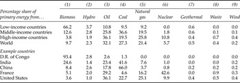
The primary energy mixes of low-, middle-, and high-income countries for the year 2010 are presented in table 1, as well as data for five representative countries (ordered from low to high GDP per capita). Low-income countries source around two-thirds of their primary energy from biomass, and 29 per cent from fossil fuels. In contrast, middle-income countries source more than four-fifths of their energy from fossil fuels, primarily coal and oil. High-income countries also source a large share of their energy from fossil fuels, but tend to be less dependent on coal than middle-income countries. High-income countries also source a larger share of their energy from nuclear power (11 per cent), and a growing share from renewables such as waste and wind. The hydro share of the energy mix tends to be lower for countries with higher incomes.
Energy mix by income grouping, 2010

Notes: World Bank (2012) country classifications are used to class countries into income groups. Data for 138 countries are used for constructing the country group averages. An ‘other’ category making up 0.3% of world energy use is not shown. This category includes energy from solar, tide, wave, ocean, other hydrocarbons, heat, electricity transfers and other sources.
Source: IEA, (2012a).
The remainder of this paper is organized as follows. Section 2 discusses potential reasons for the existence of a national-level energy ladder. Section 3 discusses the econometric estimation method and the data to be used. The results are presented in section 4. An application of the results to gain insight into how the carbon intensity of energy evolves as economies develop is presented in section 5. The final section concludes.
2. Potential reasons for a national-level energy ladder
A national-level energy ladder may emerge as a result of several sets of factors. The first of these is supply-side factors, as represented in the models of Tahvonen and Salo (Reference Tahvonen and Salo2001) and Burke (Reference Burke2010). The existence of diminishing returns to domestic energy resources (e.g., running out of rivers to dam for hydroelectricity) means that imported fuels or modern energy sources such as nuclear power become increasingly cost competitive relative to domestic energy options as incomes increase and more domestic resources are exploited (and/or depleted). Economic development also relieves capital, human capital and institutional constraints, meaning that energy sources that are capital intensive and/or require advanced human capital or energy sector institutions, such as natural gas, nuclear power and wind power, become increasingly viable as economies develop.
A national-level energy ladder may also emerge due to a positive income elasticity of demand for energy forms that are more effective, efficient, convenient, safer and/or cleaner (Grübler and Nakićenović, Reference Grübler and Nakićenović1996; Grübler, Reference Grübler2004). Consequently, higher incomes are likely to see a reorientation of demand away from locally collected biomass (which tends to be an inconvenient, labour-intensive, locally polluting energy form) towards a demand for high-quality energy forms such as electricity and petroleum. At the national level, increased incomes may also lead to a shift in demand towards higher quality energy forms such as those which are less polluting or allow enhanced energy security. In (high-income) France and Denmark, for instance, governments supported transitions to nuclear and wind power (respectively) in response to energy security and environmental issues associated with the use of fossil fuels (Hadjilambrinos, Reference Hadjilambrinos2000).
A national-level energy ladder may also be partly a result of structural change in the economy. Economic development typically sees a realignment of economic activity (and energy demand) from agriculture towards industry, transport and services, although the relative importance of industrial activity tends to fall at high income levels (Judson et al., Reference Judson, Schmalensee and Stoker1999; Medlock and Soligo, Reference Medlock and Soligo2001; Schäfer, Reference Schäfer2005). Given that sectoral energy demand is often tied to specific forms of energy, structural change as an economy develops may result in changes in the energy mix. The ascendance of the transportation sector as economies develop (Medlock and Soligo, Reference Medlock and Soligo2001), for instance, is likely to place upward pressure on the oil share of the energy mix.
Other features of economic development, such as urbanization, may also contribute to the national-level energy ladder. Urban populations are less likely to be able to collect plant matter to use for heating and cooking purposes due to a lack of proximity to forests and farms, meaning that it should be expected that urbanization reduces overall dependence on biomass energy (Barnes and Floor, Reference Barnes and Floor1999). Urban areas are also more likely to be connected to energy grids (e.g., for electricity and natural gas) given their higher population densities. The shift to urban living as economies develop may thus contribute to a switching from the use of primary biomass towards electricity and natural gas.
3. Estimation approach and data
The model for estimating the effect of per capita GDP on the primary energy mix is of the form:
 $$S_{j\comma c\comma t} =\alpha _j \ln Y_{c\comma t} +\beta _j \lpar \ln Y_{c\comma t} \rpar ^2+{\bi x^{\prime}}_{c\comma t} {\bi \chi} _j +\varepsilon _{j\comma c\comma t}$$
where the dependent variable is the proportional share (ranging from 0 to 1) of primary energy source (S) type j in total primary energy use in country c in year t, Y c, t is real GDP per capita in purchasing power parity (PPP) terms, and x′c,t is a vector of additional potential determinants of the energy mix.
ɛj,c,t is an error term, with E(ɛj,c,t)=0. The vector includes variables measuring country size (the natural logarithms of population and land area), a dummy for transition economies, and proxies for domestic energy endowments. The endowment variables include per capita: (a) forest area (as a proxy for biomass potential); (b) renewable internal freshwater resources (as a proxy for hydro power potential); (c) oil reserves; (d) coal reserves; (e) natural gas reserves; and (f) volcanoes (as a proxy for geothermal potential). I do not explicitly control for policy variables or country-specific energy prices as these are likely to be functions of underlying factors such as development level and resource endowments. I primarily focus on the average effects of GDP per capita on the energy mix shares for the full sample, but figure 1 explores results for sub-samples of fossil fuel-poor and fossil fuel-rich countries.
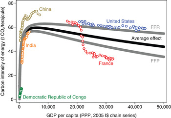
GDP per capita and the predicted carbon intensity of primary energy
Notes: The ‘average effect’ is from quadratic estimations using 1960–2010 fixed effects panel data (i.e., regressions as in table 4). FFR (fossil fuel-rich) is the average effect for the panel sub-sample of countries with fossil fuel reserves per capita exceeding the year-2010 median. FFP (fossil fuel-poor) is the average effect for the panel sub-sample of countries with fossil fuel reserves per capita below the year–2010 median. All three use the year-2010 year effect and the average of the country fixed effects. Carbon emission factors are from IPCC (1996), as used by IEA (2012b). Actual data for 1971–2010 for five representative countries are from IEA (2012b).

Estimations are carried out for separate dependent variables, measuring the shares of each of the nine energy source types in table 1 in total primary energy supply (TPES). These nine sources together accounted for 99.7 per cent of measured global TPES in 2010. (Results for a 10th source, ‘other’, are not shown.) I present ordinary least squares estimates for the cross-sectional sample and estimates using the fixed effects estimator (with year dummies) for the panel sample. Panel results using the between estimator are also discussed, and are presented in the online Appendix available at http://journals.cambridge.org/EDE. Standard errors are robust to heteroscedasticity. Unreported results using the random effects estimator are similar to those using the fixed effects estimator. The estimated income effects on the energy mix are generally similar in specifications that control for ratification of the Kyoto Protocol, precipitation and temperature (using data from Mitchell et al., Reference Mitchell, Carter, Jones, Hulme and New2004), or regional fixed effects (which partly capture cultural, climatic and other differences between countries).
Important features of the estimation approach are that it involves the use of fractional data for the dependent variables and that the estimation equations are subject to a cross-equation aggregation restriction (the dependent variables for the 10 equations sum to 1). Overall results are similar in specifications that explicitly recognize these characteristics of the data, such as compositional data analysis models (Aitchison, Reference Aitchison1986), fractional logit or fractional multinomial logit models (Papke and Wooldridge, Reference Papke and Wooldridge1996), or zero/one inflated beta models (Ferrari and Cribari-Neto, Reference Ferrari and Cribari-Neto2004). Results are also similar in Tobit models, or in logit or probit estimations (either standard or ordered). Tobit models are not suited to the inclusion of country fixed effects, but the fixed effects panel results are generally similar in estimates using the Honoré (Reference Honoré1992) semiparametric model. Results for these specifications are available on request. Because the same set of controls is included in each equation, seemingly unrelated regressions estimation provides no advantage over equation-by-equation ordinary least squares.
Regression estimations of the 10 equations must preserve an important property: the sum of the partial derivatives with respect to any explanatory variable across the 10 equations must equal zero. This applies to the partial derivative with respect to log GDP per capita in the quadratic specifications also, i.e., ∑j(αj+2βj lnY)=0, ∀c, t. I have confirmed that this property holds across all of the reported sets of estimations.
Results are presented for specifications both with and without the quadratic log GDP term. GDP per capita levels at the implied turning points are shown if the quadratic term is statistically significant at the 10 per cent level. The estimated relationships are only classed as non-monotonic (U or inverse-U shaped) if the quadratic term is statistically significant at the 10 per cent level or higher and the GDP per capita level at the estimated turning point is above I$2,000.Footnote 1
Estimations are presented for a cross-section of 134 countries for the year 2010, and a panel of 4,949 observations for the same countries for the period 1960–2010. The motivation for presenting the cross-sectional results is that data for key control variables such as fossil fuel reserves are only available for a limited number of years, and so are not suited to the long annual panel. The choice of 2010 for the cross-sectional estimations is of no particular consequence, as results are similar for other years. The countries in the sample together accounted for 95 per cent of the global population in 2010.
Energy data are from the International Energy Agency (IEA, 2012a). The IEA energy data are the best available for the current purpose, although concerns are held regarding the accuracy of the data on biomass use, which may be underreported. It is nevertheless believed that measurement error is unlikely to have any important qualitative impact on the results presented in this paper, even if the scale of the transition from biomass is potentially underestimated. GDP data are from the Penn World Table (Heston et al., Reference Heston, Summers and Aten2012). A full list of definitions and data sources is provided in the Appendix.
4. Results
4.1. Cross-sectional estimates
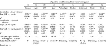
Results for estimations of equation (1) for each of the nine energy sources for the year-2010 cross-section are presented in table 2. Specification 1 includes only log GDP per capita; specification 2 also includes the squared log GDP per capita term. The specification 1 results indicate that the average income effect is negative and statistically significant for the biomass share of the primary energy mix, and positive and statistically significant for the oil, coal, natural gas, nuclear, waste and wind shares. GDP per capita on average has no significant impact on the hydro and geothermal shares of the primary energy mix in this specification. The results imply that economic development involves a large substitution away from biomass and towards commercial energy forms such as fossil fuels and electricity.
Cross-sectional results, 2010

Notes: ***, **, and * indicate statistical significance at the 1%, 5%, and 10% levels, respectively. Robust standard errors are in parentheses. Coefficients on constants are not reported. The dependent variables range from 0 to 1.
aOnly shown if the quadratic term is significant at the 10% level.
bRelationships are only classed as non-linear if the quadratic term is statistically significant at the 10% level and GDP per capita at the estimated turning point exceeds I$2,000.
Sig., significant.
The results for specification 2 in table 2 allow for non-monotonicities in the income–energy mix relations. The estimates indicate that the biomass share of the energy mix declines until a high per capita GDP level of 2005 I$41,000 is reached, from which point biomass tends to become a larger contributor to total energy use again. A biomass revival has indeed been observed in a number of high-income countries, such as Sweden which has increasingly used biomass for heating and electricity generation as well as in the form of biofuels for transport. The results also indicate that the oil and coal shares of the energy mix evolve in an inverse-U shaped manner, with peaks at per capita income levels of I$11,000 and I$15,000. This is consistent with oil and coal being on the middle rungs of the national-level energy ladder, i.e., countries substitute towards oil and coal as they develop, and then eventually start to substitute towards fuels on even higher rungs of the national-level energy ladder. The other results for specification 2 do not provide strong support for non-monotonicities.
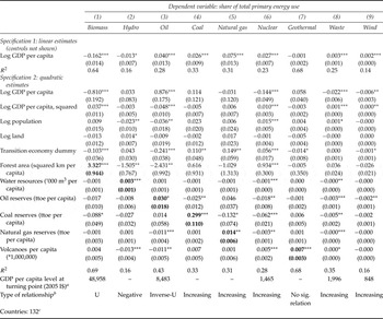
Cross-sectional results including the full set of controls are presented in table 3. These are generally similar to those in table 2, and support the conclusion that higher incomes on average result in a reduction in the biomass share of the energy mix (until very high income levels are reached), an initial increase and then decrease in the oil share of the energy mix, and continued increases in the natural gas, nuclear, waste and wind shares of the energy mix. The estimated quadratic term in the coal regression is negative but statistically insignificant at the standard levels, implying an inverse-U shape for the coal share of the energy mix, albeit one which is not precisely estimated. The coefficients of determination (R 2) are reasonably high for most of the energy source types. For instance, 69 per cent of the cross-country variation in the biomass share of the energy mix in 2010 is explained by the variables included in the model.
Cross-sectional results with controls, 2010

Notes: ***, **, and * indicate statistical significance at the 1%, 5%, and 10% levels, respectively. Robust standard errors are in parentheses. Coefficients on constants not reported. The bold diagonal is the set of own-resource coefficients. The dependent variables range from 0 to 1.
aOnly shown if the quadratic term is significant at the 10% level.
bRelationships are only classed as non-linear if the quadratic term is statistically significant at the 10% level and GDP per capita at the estimated turning point exceeds I$2,000.
cHong Kong and Taiwan are excluded due to missing resource data.
Sig., significant.
The results on the control variables provide additional information on the determinants of the primary energy mix. Countries with larger populations tend to have higher dependence on nuclear power and waste, and are less dependent on hydro and oil, holding other factors constant. Transition economies tend to be less reliant on biomass, oil, geothermal and wind energy than otherwise similar countries, and more dependent on coal, natural gas and nuclear power.
The results on the energy endowment controls are of particular interest. The bold coefficients are the own-resource coefficients and should be expected to be positive, as countries are more likely to use a particular energy resource if they have large endowments of that resource (and therefore access to it at relatively low cost). These own-resource coefficients are indeed positive, and are each statistically significant at the 10 per cent level or higher. They indicate that forested countries tend to be more dependent on biomass, countries with larger freshwater endowments tend to use more hydro power, countries with larger fossil fuel reserves are particularly dependent on these energy sources, and countries with large geothermal endowments are more likely to develop geothermal energy.
The cross-resource coefficients should be expected to be generally negative: additional endowments of any particular energy resource are likely to reduce the extent to which a country uses other energy sources. The results on the cross-resource variables indicate that bio-rich countries are indeed statistically less likely to climb off the lowest rung of the national-level energy ladder and switch to hydro power or oil. Similarly, countries with large water or fossil fuel endowments are less likely to have climbed to the upper rungs of the national-level energy ladder (nuclear power and modern renewables).
The estimated income effects are large. They suggest that a country with a per capita GDP of 2005 I$10,000 (e.g., Botswana) sources an additional 26 percentage points of its energy from fossil fuels relative to an otherwise similar country with a per capita GDP of 2005 I$2,000 (e.g., Ghana). The estimated endowment effects are also large. They imply, for instance, that the United States sources an additional 11 percentage points of its energy from coal relative to an otherwise similar country with no coal endowments.
The exogeneity of fossil fuel reserves is an issue deserving consideration: measured reserves may be affected by unobserved factors in the error term, such as economic policies or cultural preferences. As a robustness check, I ran estimates using backdated data on fossil fuel reserves for the year 1971 from Norman (Reference Norman2008). Results are generally similar using this approach, or using alternative reserves estimates from the World Resources Institute (2010).
An additional issue of concern is that GDP per capita may be correlated with variables in the error term, which would lead to biased and inconsistent estimates of the income effect on the various energy mix shares. Government policies, for instance, may affect both income and the energy mix. Alternatively, the regressions might be affected by reverse causality if a country's GDP per capita were a function of its access to certain types of energy. To explore the importance of this issue, I estimated specifications in which current log GDP per capita is instrumented with year-1950 log GDP per capita, following the approach of Burke (Reference Burke2010). This instrumental variable (IV) strategy exploits the strong persistence in GDP per capita levels over time (i.e., countries that started off with relatively high per capita incomes tend to still have relatively high per capita incomes now). The IV estimation results, presented in the supplementary materials, are generally similar to those in specification 1 of table 2. (Non-linear IV estimates are not explored because they can be unreliable; Angrist and Krueger, Reference Angrist and Krueger2001.) An additional strategy to reduce the potential for omitted-variable bias, pursued next, is to control for country-specific fixed effects.
4.2. Panel estimates
Fixed effects panel estimates for the period 1960–2010 are shown in table 4. The estimates include time dummies, and so control for time-specific factors in addition to country-specific factors. Time-specific factors may include changes in global energy prices, technologies and perceptions of nuclear safety and energy security. Country-specific factors may include time-invariant aspects of preferences, policies, institutions, economies, climate, geography, culture and energy security risks.
Fixed effects panel estimates
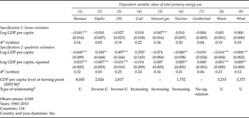
Notes: ***, **, and * indicate statistical significance at the 1%, 5%, and 10% levels, respectively. Standard errors, robust to heteroscedasticity, are in parentheses. Coefficients on constants and year dummies are not reported. The within-R 2 reflects the explanatory power of the GDP per capita terms and the year dummies. The dependent variables range from 0 to 1.
aOnly shown if the quadratic term is significant at the 10% level.
bRelationships are only classed as non-linear if the quadratic term is statistically significant at the 10% level and GDP per capita at the estimated turning point exceeds I$2,000.
Sig., significant.
The results in table 4 generally concur with the cross-sectional results, although some details differ. The estimates indicate that biomass dependence tends to decrease as countries move out of the lowest development levels, until a per capita GDP of around I$8,000 is reached. The results also indicate that economic development results in an initial increase in the hydro share of the energy mix, but that this starts to fall from a GDP per capita level of I$2,000. The oil share of the energy mix is estimated to peak at a GDP per capita of around I$3,000 (a lower turning point than in the earlier estimations), and the fixed effects estimates continue to indicate that long-run economic growth results in increases in the natural gas, nuclear, waste and wind shares of the energy mix over most income levels. As in the cross-sectional results with the control variables (table 3), the quadratic term in the coal equation is outside the standard significance levels in the fixed effects specification (p=0.14). The estimate points to an initially increasing and then, from middle-income levels, a decreasing relationship between per capita GDP and the coal share of the energy mix, although the curvature of the relationship is not precisely estimated.
The between estimator can provide consistent estimates of long-run relationships given standard assumptions about the error term and its relationship with the explanatory variables (Stern, Reference Stern2010). Results using this estimator are presented in the online Appendix. They are similar to the cross-sectional results, providing support to the finding that economic development results in a falling biomass share of the energy mix (until high income levels are reached), an inverse-U shaped oil share of the energy mix, and increasing natural gas, nuclear, waste and wind shares.
5. Application of the national-level energy ladder results to carbon emissions trajectories
Taken together, the results support the existence of a national-level energy ladder that countries climb as their per capita incomes increase, and are consistent with the implications of the energy transition models of Tahvonen and Salo (Reference Tahvonen and Salo2001) and Burke (Reference Burke2010), and earlier evidence on aggregate energy transitions from authors such as Grübler (Reference Grübler2004). An interesting application of the results is to examine their implications for the evolution of the carbon intensity of energy as economies develop. While total CO2 emissions are what end up mattering to the atmosphere, it is useful to examine how the carbon intensity of energy evolves as economies develop in order to understand the underlying factors affecting total CO2 emissions.
Figure 1 shows the implied average carbon intensity of energy based on predictions from the fixed effects panel regressions in table 4, plotted against GDP per capita. The carbon intensity of energy is a weighted average of the carbon intensities of individual energy types. Here, the implied carbon intensity of energy is calculated by applying the Intergovernmental Panel on Climate Change (IPCC, 1996) carbon factors to each of the energy source types.Footnote 2 Following IPCC and IEA practice, only emissions from the three fossil fuels (oil, coal, natural gas) are included; it is assumed that biomass is used sustainably and so is associated with no net carbon emissions. The predictions use the year-2010 time fixed effect (i.e., are for year-2010 technology and prices), and are for a country with average values of the country fixed effect.
Figure 1 shows three regression predictions. The ‘average effect’ is for the full sample of countries, and shows that the carbon intensity of energy increases as countries proceed through the initial development stages, before peaking and then declining as countries enter the middle- and high-income categories. The estimated turning point is at a GDP per capita level of I$6,000, the year-2010 level of Guatemala. The initial increase is mostly caused by the documented substitution away from biomass and towards fossil fuels. The subsequent decrease in the carbon intensity of energy use is caused by a substitution away from the most carbon-intensive fossil fuels (coal and oil) towards natural gas, nuclear power and modern renewables (including a return to the use of biomass).
It was observed in table 3 that countries with large fossil fuel reserves are (a) more likely to use fossil fuel energy, and (b) less likely to climb to the upper rungs of the national-level energy ladder by transitioning to nuclear power and modern renewables. These findings imply that we should expect some resource-induced heterogeneity in the relationship between the carbon intensity of energy and GDP per capita. The ‘FFP’ line in figure 1 represents the average effect for the sub-sample of ‘fossil fuel-poor’ countries, defined as those with below-median fossil fuel reserves per capita in 2010. The ‘FFR’ line represents the average effect for the sub-sample of ‘fossil fuel-rich’ countries, defined as those with above-median fossil fuel reserves per capita in 2010. It can be seen that the carbon intensity of energy typically rises to a higher level in fossil fuel-rich countries, and exhibits a slower decline as countries continue to develop. Fossil fuel-poor countries experience larger declines in the carbon intensity of energy due to their greater adoption of upper-rung technologies such as nuclear power and modern renewables.
Figure 1 shows observed IEA (2012b) carbon intensity of energy data for the five countries listed in table 1. The Democratic Republic of the Congo has a very low GDP per capita level, and mostly uses biomass, so is at the base of the chart. India's rapid growth over recent years has seen it become increasingly dependent on fossil fuels, and as a consequence its carbon intensity of energy has increased in a way which aligns very closely to the predictions emerging from this paper's energy share regression results. India's relatively large coal reserves place it among the ‘fossil fuel-rich’ sub-sample, implying that the carbon intensity of India's energy is likely to continue to increase for the next decade at least. China, on the other hand, has a high carbon intensity of energy, and one which is likely to continue to decrease as its economy grows. France is among the fossil fuel-poor countries, and has seen a very large reduction in its carbon intensity of energy as it has substituted away from oil and coal and towards natural gas and nuclear power. Finally, the United States is tracking very close to the average carbon intensity of energy of the sub-group of countries with above-median per capita fossil fuel reserves. The results of this paper indicate that the carbon intensity of energy in the United States is likely to maintain its gradual decline as the country continues to substitute to natural gas and low-carbon energy sources on the upper rungs of the national-level energy ladder.
Numerous studies have noted that the carbon intensity of primary energy has fallen over time in developed countries (Grübler and Nakićenović, Reference Grübler and Nakićenović1996; Nakićenović, Reference Nakićenović1996a, Reference Nakićenović1996b; Schipper et al., Reference Schipper, Ting, Khrushch and Golove1997; Grübler et al., Reference Grübler, Nakićenović and Victor1999a; Grübler et al., Reference Grübler, Nakićenović and Victor1999b; Nakićenović and Grübler, Reference Nakićenović and Grübler2000; Jotzo et al., Reference Jotzo, Burke, Wood, Macintosh and Stern2012). The results in this paper help to clarify that this decarbonization is a direct product of changes in energy mix as countries climb the national-level energy ladder. The results on the importance of fossil fuel resource endowments accord with those of Burke (Reference Burke2012), who finds that fossil fuel-rich countries are much more likely to experience reductions in CO2 emissions per capita as they develop than are fossil fuel-poor countries.
6. Conclusions
This paper has presented evidence from a large sample of countries for the years 1960–2010 on the existence of a national-level energy ladder that countries climb as they develop. Economic development typically sees countries switch from biomass towards commercial fossil fuels, and also some hydroelectricity. At higher income levels, countries increasingly adopt low-carbon energy sources such as nuclear power and certain modern renewables such as wind power. In terms of carbon emissions, the net effect is that economic development typically causes an initial carbonization, and a later decarbonization, of the energy system.
The results indicate that not all countries climb the ladder in the same manner, however. Countries with large endowments of any energy source are less likely to continue climbing to higher rungs of the national-level energy ladder. Fossil fuel-rich countries are much less likely to adopt nuclear power and modern renewables, and to achieve reductions in the carbon intensity of their energy, as they reach high income levels.
A large share of the world's population lives in countries that are still on the upward slope of the carbon intensity of energy curve, where energy systems are likely to become increasingly dependent on carbon-intensive fossil fuels as per capita incomes increase. The carbon intensity of energy use in Myanmar, for instance, is only one-quarter of the world average, and would likely increase substantially if sustained economic development were to be experienced in the country. There is some brighter news on China: the results imply that the carbon intensity of China's energy use is likely to reduce over coming years as China reorientates its energy mix towards natural gas, nuclear power and renewable energy. A decline in China's carbon intensity of energy will likely be coupled with a large increase in energy use, however, meaning that China's overall emissions of CO2 from energy are likely to continue to rise for the foreseeable future.
Efforts to encourage leapfrogging to the lower-carbon energy sources on the upper rungs of the national-level energy ladder (modern renewables, nuclear power and also natural gas), where appropriate, is one potential means to reduce the magnitudes of the upticks in the carbon intensity of energy and total CO2 emissions expected for many developing countries. Carbon pricing and the removal of fossil fuel subsidies would help to facilitate such leapfrogging. There may also be a role for developed countries to provide additional assistance to developing countries to aid their early adoption of low-carbon energy sources and technologies.
The results also draw attention to the formidable challenge of weaning fossil fuel-rich countries off their dependence on carbon-intensive fossil fuels, as even at high income levels these countries tend to remain heavily reliant on fossil fuels for their energy needs. The development of affordable lower-carbon fossil fuel energy technologies is likely to be an indispensable part of an optimal climate change mitigation response.
Appendix: Variable descriptions
Biomass share of total primary energy use: biomass and biofuels share of TPES (IEA, 2012a).
Hydro share of total primary energy use: hydro share of TPES (IEA, 2012a).
Oil share of total primary energy use: crude oil and petroleum share of TPES (IEA, 2012a).
Coal share of total primary energy use: Coal and peat share of TPES (IEA, 2012a).
Natural gas share of total primary energy use: natural gas share of TPES (IEA, 2012a).
Nuclear share of total primary energy use: nuclear share of TPES (IEA, 2012a).
Geothermal share of total primary energy use: geothermal share of TPES (IEA, 2012a).
Waste share of total primary energy use: use of industrial and municipal waste for energy, share of TPES (IEA, 2012a).
Wind share of total primary energy use: wind share of TPES (IEA, 2012a).
Log GDP per capita: natural logarithm of GDP per capita in 2005 international $ (I$), chain series (Heston et al., 2012a).
Log population: natural logarithm of population (Heston et al., Reference Heston, Summers and Aten2012).
Log land: natural logarithm of land area in squared kilometres (World Bank, 2012).
Transition economy dummy: 1 for countries classed as transition economies; 0 otherwise (Development Research Institute, 2008).
Forest area (squared km per capita): land under natural or planted stands of trees of at least 5 m in situ, excluding trees in agricultural production systems or urban parks and gardens (World Bank, 2012). Population data from Heston et al. (Reference Heston, Summers and Aten2012).
Water resources (thousand cubic meters per capita): renewable internal freshwater resources (internal river flows and groundwater from rainfall) in thousand cubic meters per capita. Data are for 2009 (World bank, 2012). Data for Serbia are from FAO (2012), and are used for Montenegro as well.
Oil reserves (thousand tonnes oil equivalent [ttoe] per capita): proved reserves of crude oil (US EIA, 2012). BP (2012) conversion factors are used. Countries for which data are not available are considered to have zero reserves. Population data from Heston et al. (Reference Heston, Summers and Aten2012).
Coal reserves (ttoe per capita): total recoverable coal reserves. Data are for 2008 (US EIA, 2012). Converted to ttoe using BP (2012) conversion factors. Countries for which data are not available are considered to have zero reserves. Population data from Heston et al. (Reference Heston, Summers and Aten2012).
Natural gas reserves (ttoe per capita): proved reserves of natural gas (US EIA, 2012). Converted to ttoe using BP (2012) conversion factors. Countries for which data are not available are considered to have zero reserves. Population data from Heston et al. (Reference Heston, Summers and Aten2012).
Volcanoes per capita (*1,000,000): number of holocene volcanoes*1,000,000, divided by population. Volcanoes straddling national borders are included in the list of volcanoes of all border countries (siebert and Simkin, Reference Siebert and Simkin2002). Population data from Heston et al. (Reference Heston, Summers and Aten2012).