


1. Introduction
Plane Couette (PC) flow refers to the motion of a Newtonian fluid between two parallel flat plates spaced a distance  $2h$ apart that move in opposite directions, each with speed
 $U_c$. Although PC flow is difficult to study experimentally (see Kitoh, Nakabyashi & Nishimura Reference Kitoh, Nakabyashi and Nishimura2005; Kitoh & Umeki Reference Kitoh and Umeki2008), owing to the presence of large-scale roll structures, it remains a canonical flow configuration in both theoretical fluid mechanics and in the computational study of turbulent, wall-bounded flows. Unlike Poiseuille-channel flow where the mean skin-friction is determined by the driving pressure gradient, for PC flow, the plate Reynolds number
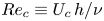 $Re_c \equiv U_c\,h/\nu$ (
 $\nu$ the fluid kinematic viscosity) is generally specified and the frictional Reynolds number
 $Re_\tau \equiv u_\tau h /\nu$, with
 $u_\tau$ the skin-friction velocity, must be determined as a function of
 $Re_c$.
Numerical studies of PC flow appear presently to be restricted to DNS. These include Bech et al. (Reference Bech, Tillmark, Alfredsson and Andersson1995), Komminaho, Lundbladh & Johansson (Reference Komminaho, Lundbladh and Johansson1996), Tsukahara, Kawamura & Shingai (Reference Tsukahara, Kawamura and Shingai2006) and Pirozzoli, Bernardini & Orlandi (Reference Pirozzoli, Bernardini and Orlandi2011), who observed interesting properties of streamwise roll structures at moderate  $Re_c$. The DNS of Avsarkisov et al. (Reference Avsarkisov, Hoyas, Oberlack and García-Galache2014) achieved
 $Re_\tau$ from
 $125$ to
 $550$ while Lee & Moser (Reference Lee and Moser2018) studied streamwise structures at
 $Re_\tau =220$ and
 $500$, and the DNS of Pirozzoli, Bernardini & Orlandi (Reference Pirozzoli, Bernardini and Orlandi2014) reached
 $Re_\tau = 986$. In comparison, DNS of Poiseuille-channel flow has been performed up to
 $Re_\tau =5200$ by Lee & Moser (Reference Lee and Moser2015). One reason for this difference is that PC flow contains streamwise-oriented rolls, distributed in counter-rotating pairs across the spanwise domain whose resolution requires extended computational coverage in both the spanwise and streamwise directions.
Direct numerical simulations at  $Re_\tau = 180\text {--}550$ by Avsarkisov et al. (Reference Avsarkisov, Hoyas, Oberlack and García-Galache2014) shows a logarithmic layer in the mean-velocity profile with a consistent slope constant
 $0.41$, while indicating uncertain scaling of streamwise turbulent intensities in wall units. Pirozzoli et al. (Reference Pirozzoli, Bernardini and Orlandi2014) consider
 $Re_\tau \gtrsim 500$ as the start of an asymptotic, high-Reynolds regime where a secondary outer peak in the streamwise turbulent intensity is observed at around a wall normal distance
 $y/h=0.3$ for
 $Re_\tau \approx 1000$. According to their spectral signature, this secondary peak is related to the presence of large-scale rolls of spanwise extent with approximately five half-channel-heights. A concern is that an effect of spanwise periodicity may persist owing to nominally infinite spanwise correlation lengths for some second-order turbulent statistics.
In assessing the effect of the streamwise domain size, Lee & Moser (Reference Lee and Moser2018) show that for low  $Re_\tau$, streamwise rolls can be inclined from the streamwise direction by up to
 $4^{\circ }$. They also observe coherent spanwise structures with increasing streamwise coherence length with increasing
 $Re_\tau$. For their largest
 $Re_\tau =500$, this inclination is not observed which may be a result of insufficient streamwise domain size. Their one-point statistics show no significant difference between small and larger domain DNS for all three
 $Re_\tau$ investigated.
As a standard numerical simulation tool, large-eddy simulation (LES) is implemented on a grid that is too coarse for full DNS resolution. In wall-resolved LES (WRLES), small-scale dynamics are modelled using a subgrid-scale (SGS) model away from walls but the viscous wall scale  $\delta _\nu \equiv \nu /u_\tau$ is resolved in the wall-normal direction at least near the wall. According to Choi & Moin (Reference Choi and Moin2012), the computational resource required for successful WRLES scales as
 $O(Re^{13/7})$, which is small compared with the DNS requirement of
 $O(Re^{37/14})$. In wall-modelled LES (WMLES), a further step is taken with the implementation of a so-called wall model generally designed to recognize but not resolve
 $\delta _\nu$, while still capturing essential near-wall physics and also providing a suitable modified boundary condition for the outer flow. The purpose of WMLES is to achieve larger
 $Re_\tau$ than can be reached with either DNS or WRLES and also to limit computational resource to at most a weak function of an appropriate Reynolds number.
The viability of wall-resolved LES of canonical turbulent flows has been well established, for example in Poiseuille-channel flow (Moin & Kim Reference Moin and Kim1982). Further, channel flow has become a benchmark case for developing new SGS and wall models, such as the stretched-spiral vortex model (Voelkl, Pullin & Chan Reference Voelkl, Pullin and Chan2000; Chung & Pullin Reference Chung and Pullin2009) or the variational, multiscale LES approach (Hughes, Oberai & Mazzei Reference Hughes, Oberai and Mazzei2001). While WRLES of Poiseuille flow has been largely successful, its application to flows with moving boundaries, such as PC flow or Taylor–Couette flow, has received little attention.
Wall-modelled LES, which requires both an SGS model and a wall model, has also been applied to canonical wall-bounded turbulent flows for example the virtual-wall model (VWM; Chung & Pullin Reference Chung and Pullin2009), the integral model (Yang et al. Reference Yang, Sadique, Mittal and Meneveau2015) and the slip-boundary condition model (Bae et al. Reference Bae, Lozano-Durán, Bose and Moin2019). WMLES has shown potential to provide flow simulation at extreme Reynolds numbers including Poiseuille channel flow up to  $Re_\tau \sim 10^7$ and flat-plate, equilibrium boundary-layer flow with
 $Re_\tau$ up to
 $10^{11}$ (Inoue & Pullin Reference Inoue and Pullin2011). Cheng, Pullin & Samtaney (Reference Cheng, Pullin and Samtaney2015) demonstrated WMLES for a separating–reattaching turbulent boundary layer at large
 $Re_\tau$. Gao, Cheng & Samtaney (Reference Gao, Cheng and Samtaney2020) further performed WMLES of flow in a channel with periodic hills (also with separation/reattachment). This suggests that WMLES could capture large-scale streamwise structures exhibiting flow separation/reattachment in turbulent PC flow.
The goal of the present study is to investigate PC flow using both WRLES and WMLES up to  $Re_c \sim 10^7$, which corresponds to
 $Re_\tau \sim 2.8\times 10^5$. In the following, in § 2, we briefly describe the numerical method and physical models employed, including the SGS and wall models. Then in § 3, we outline the simulations performed including DNS, WRLES and WMLES. Code verification for LES of PC flow is discussed in detail. In § 4, we show results of WRLES up to
 $Re_\tau \approx 3600$, which include spanwise- and timewise-averaged mean velocity profiles and turbulent intensities in both inner and outer scales, to explore the
 $Re_c$ dependence on the structure of the turbulent wall layers. The spanwise velocity variation produced by the presence of streamwise rolls is discussed in § 5. Attention is focused on WMLES of PC flow in § 6, starting with
 $Re_\tau \approx 3600$, which overlaps the range of the WRLES, and extending to
 $Re_\tau \approx 2.8 \times 10^{5}$. The discussion includes classical turbulence properties, such as the
 $Re_\tau -Re_c$ relationship, scaled velocity gradients in § 7 and roll diagnostics in § 8. A brief summary is provided in § 9.
2. Numerical method and physical model
2.1. Numerical method
Plane Couette flow is numerically simulated through discretization of the incompressible, constant viscosity Navier–Stokes (N–S) equations in a Cartesian coordinate box. In LES, a general filter with size  $\varDelta _c$ is applied to the N–S equation, which results in
 \begin{equation} \frac{\partial \widetilde{u_i}}{\partial t} + \frac{\partial \widetilde{u_i} \widetilde{u_j}}{\partial x_j} ={-} \frac{1}{\rho} \frac{\partial \tilde{p}}{ \partial x_i} + \nu \frac{\partial^2 \widetilde{u_i}}{\partial x_j^2} - \frac{\partial T_{ij}}{\partial x_j}, \quad \frac{\partial \widetilde{u_i}}{\partial x_i} = 0. \end{equation}
Here  $\widetilde {u_i}$ is the filtered velocity,
 $\rho$ the density and
 $\tilde {p}$ the filtered pressure. Additionally,
 $T_{ij}= \widetilde {u_iu_j}- \widetilde {u_i}\widetilde {u_j}$ denotes the effect of unresolved scales on the resolved-scale motion, which is modelled by an SGS model.
The computational box is set up with dimensions  $L_x \times L_y \times L_z$ with periodic boundary conditions in both the streamwise (
 $x$-) and spanwise (
 $z$-) directions, and corresponding mesh
 $N_x \times N_y \times N_z$. The mesh is uniform in the
 $x$- and
 $z$-directions. In the wall-normal
 $y$-direction, the mesh is stretched for WRLES but uniform for WMLES. The stretching function employed is that used by Pirozzoli et al. (Reference Pirozzoli, Bernardini and Orlandi2014), namely an error function mapping
 $\textrm {erf}(\alpha \xi /2)/\textrm {erf}(\alpha /2)$ with
 $\alpha =4$ and
 $\xi$ varying in
 $[-1,1]$. Corresponding velocity components are
 $u$,
 $v$ and
 $w$ in the
 $x$-,
 $y$- and
 $z$-directions, respectively. Moving both walls in the streamwise direction with equal and opposite speeds
 $\pm U_c$ generates the flow.
The governing equations are solved using a third-order Runge–Kutta method for time evolution with a fractional-step method for marching Eulerian velocities. The code is an extension of that used by Inoue & Pullin (Reference Inoue and Pullin2011). In solving the velocity-update equation, only the wall-normal viscous term is treated implicitly and the wall-parallel viscous terms are treated explicitly. The skew-symmetric form of the nonlinear term is employed. For spatial discretization, a Fourier spectral method is used in the streamwise ( $x$-) direction, while a fourth-order finite-difference method on a staggered grid is used in the other two directions. The pressure Poisson equation reduces to a sequence of two-dimensional modified Helmholtz equations in the
 $y$–
 $z$ plane and is further reduced to a one-dimensional linear system by applying a Fourier transform in the spanwise
 $z$-direction. A septa-diagonal matrix solver (from LAPACK) is used for solving the resulting equations in the wall-normal
 $y$-direction. For code parallelization, we use MPI in only the streamwise direction.
2.2. Subgrid-scale model
In the present LES, unresolved subgrid motions are represented by the stretched-vortex (SV) SGS model (Misra & Pullin Reference Misra and Pullin1997; Chung & Pullin Reference Chung and Pullin2009). More specifically, in a numerical cell, the unresolved subgrid motion is modelled by a stretched-spiral vortex (Lundgren Reference Lundgren1982) within each cell with direction vector  $ {\boldsymbol e}^v$, resulting in the subgrid stress,
 \begin{equation} T_{ij} =(\delta_{ij} - {\boldsymbol e}_i^v {\boldsymbol e}_j^v) K, \end{equation}
where  $K$ is the subgrid kinetic energy. This is computed from an integral of the stretched-spiral vortex energy spectrum
 $E(k)$ as
 \begin{equation} K=\int_{k_c}^\infty E(k) \,\textrm{d}k = \frac{\mathscr{K}'_0}{2} \varGamma\left[{-}1/3, \frac{2\nu k_c^2}{3|\tilde{a}|}\right]. \end{equation}
Here  $k_c={\rm \pi} /\varDelta _c$ is the cutoff wavenumber,
 $\tilde {a}= {\boldsymbol e}_i^v {\boldsymbol e}_j^v \tilde {S}_{ij}$ is the stretching along the subgrid vortex with
 $\tilde {S}_{ij}$ the local resolved-scale, rate-of-strain tensor. In the present implementation, the
 ${\boldsymbol e}_j^v$ are aligned with the principal extensional eigenvector of
 $\tilde {S}_{ij}$. The grouped constant
 $\mathscr {K}'_0$ is calculated dynamically from the resolved-scale velocity. The model implementation is dynamic with no adjustable parameters except that
 $\varDelta _c$ is taken as the local cell size. For details, see Misra & Pullin (Reference Misra and Pullin1997), Voelkl et al. (Reference Voelkl, Pullin and Chan2000), Chung & Pullin (Reference Chung and Pullin2009) and Lundgren (Reference Lundgren1982). In DNS and WRLES, non-slip boundary conditions are applied on both walls.
2.3. Virtual wall model for WMLES
In WRLES, the skin-friction velocity is calculated directly from the wall-normal gradient of the wall-parallel velocity evaluated at the wall. A one-sided, four-point stencil is used as described by (2.12) of Cheng et al. (Reference Cheng, Pullin, Samtaney, Zhang and Gao2017). Because the near-wall flow is not resolved in WMLES, the local skin-friction velocity must be otherwise determined.
For WMLES, we use the two-tier, VWM (Chung & Pullin Reference Chung and Pullin2009). First, an assumption of local inner scaling on  $u_\tau$ and
 $\delta _\nu$ is used in the wall-normal-average (over a thin layer
 $0< y< h_0$) of the wall-parallel, streamwise momentum equation. This gives an ordinary differential equation (ODE) describing
 $u_\tau (x,z,t)$ at each wall point. Each ODE is coupled to the outer-flow LES through the instantaneous flow state at the ‘virtual-wall’ interface at
 $y=h_0$ of the wall-modelled layer and the outer-flow LES. This locally determined
 $u_\tau$ is then used together with a log-linear-based approximation to provide a slip velocity at the virtual wall
 $y=h_0$, with dynamical evaluation of the local Kármán constant. The virtual-wall height parameter
 $h_0$ is subgrid and must be smaller than the wall-adjacent, wall-normal cell size
 $\Delta y$. Presently, we use
 $h_0 = 0.18\,\Delta y$ as suggested by Chung & Pullin (Reference Chung and Pullin2009) following a sensitivity study. Near-wall RANS is not required and
 $u_\tau (x,y,t)$ is determined dynamically. Hence
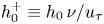 $h_0^+ \equiv h_0\,\nu /u_\tau$ is determined dynamically.
In the second part, a streamwise slip-velocity boundary condition at  $y=h_0$ is calculated, with the velocity relative to the wall given as
 \begin{equation} \tilde{u} (h_0^+) = u_\tau \left( \frac{1}{\kappa} \log \left( \frac{h_0^+}{h_\nu^+} \right) +A \right), \end{equation}
with
 \begin{equation} A = h_v^+{-} \frac{ \log h_\nu^+} {\kappa} , \quad \kappa = \frac{\gamma K^{1/2}}{2 ({-}T_{xy}/ u_\tau)} . \end{equation}
Here  $\gamma$ is a constant parameter which is estimated via Townsend's structure parameter (Chung & Pullin Reference Chung and Pullin2009). Additionally,
 $h_\nu ^+ = 10.2$ is an empirical parameter which is essentially the intersection point between the near-wall, linear and log profiles. Similar wall-normal averaging of the continuity equation provides a wall-normal velocity at
 $y=h_0$. These velocity components provide virtual-wall, Dirichlet boundary conditions for the outer-flow LES. See Chung & Pullin (Reference Chung and Pullin2009) and Cheng et al. (Reference Cheng, Pullin and Samtaney2015) for further details. The WMLES code has been verified in previous studies by comparison with DNS and experiments on flat-plate boundary layer flow (Inoue & Pullin Reference Inoue and Pullin2011) and separation/reattachment flow (Cheng et al. Reference Cheng, Pullin and Samtaney2015). In subsequent sections, we will provide further code verification for PC flow.
3. Flow simulation design and DNS/LES verification
3.1. Cases implemented
For PC flow, the single driving dimensionless parameter is  $Re_c$, and
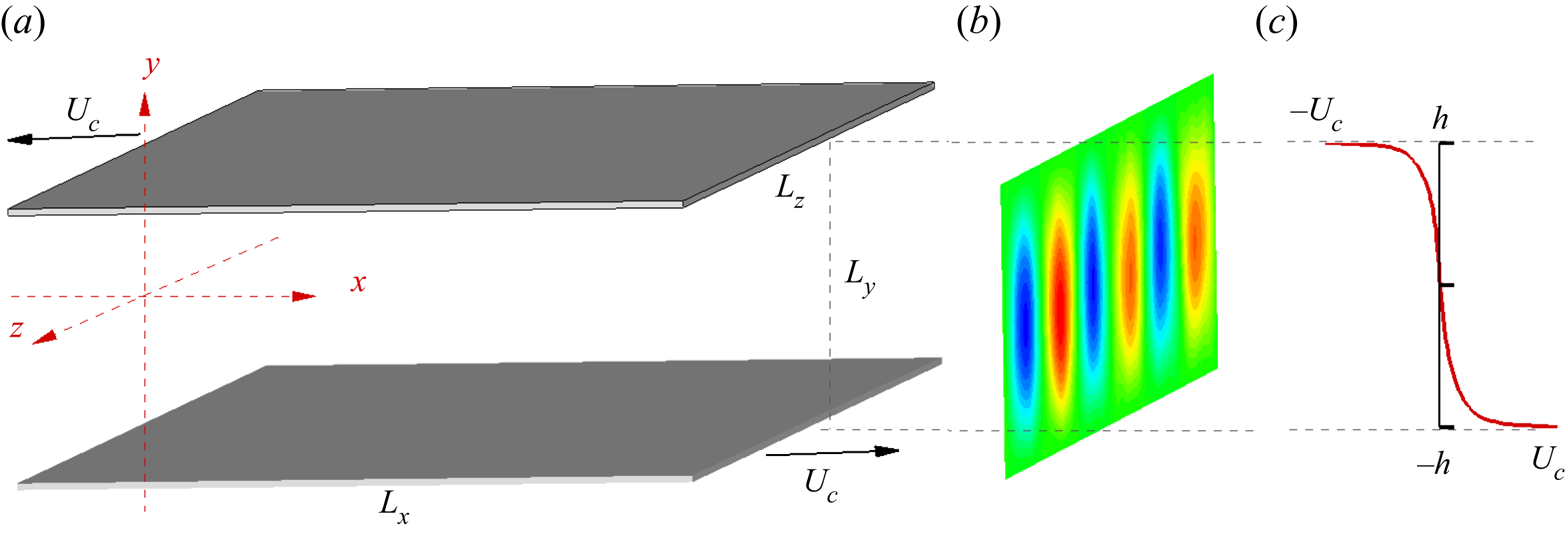
 $Re_\tau (Re_c)$ must be determined. Other parameters quantify the size and aspect ratio of the simulation domain and the grid resolution. In figure 1(a), we show a schematic of PC flow with two parallel plates, separated by
 $L_y=2h$, moving in the
 $\pm x$-directions with equal speed
 $U_c$. A sketch of a
 $(y\text {--}z)$ cross-section of the colour-contoured, streamwise averaged, wall-normal velocity is shown in figure 1(a). A stream-wise velocity profile, averaged in both the streamwise and spanwise directions is shown in figure 1(c) to illustrate the distribution of mass flux for PC flow. The present code implementation guarantees that the mass flux in both wall-parallel directions is always zero, which implies a dynamic mean pressure gradient fluctuating around zero. A test case that fixes a zero mean pressure gradient while allowing fluctuating mass flux at
 $Re_\tau \approx 500$ was also carried out. Little difference was observed on the present diagnostic results between the two methods. We will discuss the LES results in terms of
 $Re_\tau$ variation as this provides a clearer contact with other canonical flows such as Poiseuille-channel and pipe flow.
Sketch of PC flow. (a) Two parallel walls with separation distance  $L_y = 2h$. Upper and lower walls move with velocity
 $\pm U_c$. (b) Visualizing rolls via contours of streamwise averaged spanwise velocity components on a
 $(y\text {--}z)$ plane. (c) Distribution of streamwise mean velocity (averaged in both streamwise and spanwise directions).

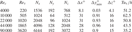
Verification begins with the DNS of Lee & Moser (Reference Lee and Moser2018) at low Reynolds number  $Re_c = 4000$ (
 $Re_\tau \approx 220$) within a domain of
 $(L_x, L_y, L_z) = (20{\rm \pi} h, 2h, 5{\rm \pi} h)$. This domain is also used later for some LES. We then implement WRLES at
 $Re_c = 10\,000$ (
 $Re_\tau \approx 500$) and
 $Re_c = 22\,000$ (
 $Re_\tau \approx 1000$) to demonstrate the SGS model capability for capturing turbulence in both the resolved, near-wall and the outer modelled domain sectors. Wall-resolved LES of two other flows with moderately large
 $Re_c=44\,000$, 90 000 are then discussed.
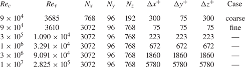
Wall-modelled LES at  $Re_c= 90\,000$, with different meshes, overlaps the WRLES and provides assessment of the VWM performance. At these
 $Re_c$, the nearest wall-normal grid point approaches the lower limit of the log region. Wall-modelled LES with
 $Re_c = 3\times 10^5$,
 $10^6$,
 $3\times 10^6$ and
 $10^7$ are then described. All cases are listed in table 1 for WRLES and table 2 for WMLES. We list prescribed parameters
 $Re_c$, mesh resolution
 $N_x \times N_y \times N_z$, the calculated
 $Re_\tau$ and the mesh size in near-wall scaling against
 $\delta _\nu$:
 $\Delta x^+$ and
 $\Delta z^+$. In the wall-normal direction, we show the minimal
 $\Delta y^+_{min}$ for WRLES and the uniform
 $\Delta _y^+$ for WMLES. The time duration used for averaging results is also shown, defined as
 $T u_\tau /h$, which represents a streamwise distance travelled with speed
 $u_\tau$. In table 2, for
 $Re_c=9\times 10^4$, two different resolutions are shown:
 $768 \times 96 \times 192$ and
 $3072 \times 96 \times 768$ referred to subsequently as coarse-mesh and fine-mesh WMLES, respectively. Results using both resolutions will be discussed later in relation to resolution requirements for the WMLES capture of spanwise roll structures.
Cases implemented in wall-resolved LES. Here,  $N_x, N_y,N_z$ are mesh resolutions in the streamwise, wall-normal and spanwise directions, respectively. Additionally,
 $\Delta x^+, \Delta y^+,\Delta z^+$ are cell sizes scaled on
 $\delta _\nu$ and
 $T\,u_\tau /h$ is the time window for time averaging.

Cases implemented for wall-modelled LES. For the key, see table 1. Here,  $Tu_\tau /h \approx 50.0$ for all cases. In the discussion, WMLES with
 $768 \times 96 \times 192$ will be referred as ‘coarse-mesh’ while WMLES with
 $3072 \times 96 \times 768$ will be denoted as ‘fine-mesh’.

3.2. Diagnostics
Owing to the existence of spanwise rolls, the spanwise direction is not homogeneous, which leads to distinct averaging methods. Two averages are defined, the first including streamwise, spanwise and time averaging, and the second that excludes the spanwise average to recognize the roll structure. We define the following two averaging operators for any instantaneous field  $\phi (x,y,z,t)$:
 \begin{equation} \bar{\phi}(y) = \frac{1}{N_t} \frac{1}{N_x} \frac{1}{N_z} \sum_{z,x,t} \phi(x,y,z,t), \quad \tilde{\phi}(y,z) = \frac{1}{N_t} \frac{1}{N_x} \sum_{x,t} \phi(x,y,z,t), \end{equation}
where  $N_t$ is the number of time steps. From instantaneous flow fields
 $u(x,y,z,t)$,
 $v(x,y,z,t)$ and
 $w(x,y,z,t)$, noting that
 $\bar {v}(y)=0$ and
 $\bar {w}(y)=0$, this allows computation of one-dimensional profiles
 $\bar {u}(y)$ and two-dimensional fields
 $\tilde {u}(y,z)$,
 $\tilde {v}(y,z)$ and
 $\tilde {w}(y,z)$.
The fluctuation part of the field can also be defined in two ways:
 \begin{equation} \phi'(x,y,z,t) = \phi(x,y,z,t) - \bar{\phi}(y), \quad \phi^\bullet (x,y,z,t) = \phi(x,y,z,t) - \tilde{\phi}(y,z). \end{equation}
Further applying the averaging operators to velocity fluctuation components results in distinct Reynolds-stress distributions. The ‘ $\bar {\phi }$’ operator produces functions of
 $y$ only,
 $\overline {u_i'u_j'}(y)$ and
 $\overline {u_i^\bullet u_j^\bullet }(y)$, while the ‘
 $\tilde {\phi }$’ operator generates fluctuation fields that are functions of
 $(y,z)$, namely
 $\widetilde {u_i'u_j'}(y,z)$ and
 $\widetilde {u_i^\bullet u_j^\bullet }(y,z)$ where
 $u_i$ and
 $u_j$ with
 $i,j=1,2,3$ could be velocity components
 $u$,
 $v$ or
 $w$.
We refer to both inner and outer length scaling  $y^+ = y/\delta _\nu$ and
 $y/h$, respectively, and corresponding velocity scales
 $u_\tau$ and
 $U_c$. We use the following notation for inner scaling:
 \begin{equation} U^+{=} \frac{ \bar{u}} {u_\tau}, \quad \left( u'u'\right)^+{=} \frac{ \overline{u'u'}}{u_\tau^2}, \quad \left( u^\bullet u^\bullet \right)^+{=} \frac{ \overline{u^\bullet u^\bullet }}{u_\tau^2}, \end{equation}
which is also applicable to other Reynolds stresses. Additional scalings, such as 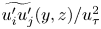 $\widetilde {u_i'u_j'}(y,z) / u_\tau ^2$ and
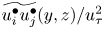 $\widetilde {u_i^\bullet u_j^\bullet }(y,z)/ u_\tau ^2$, will be described as required. In what follows, profiles of the mean velocity will refer to the mean-velocity magnitude relative to a moving wall.
3.3. Verification of DNS and wall-resolved LES
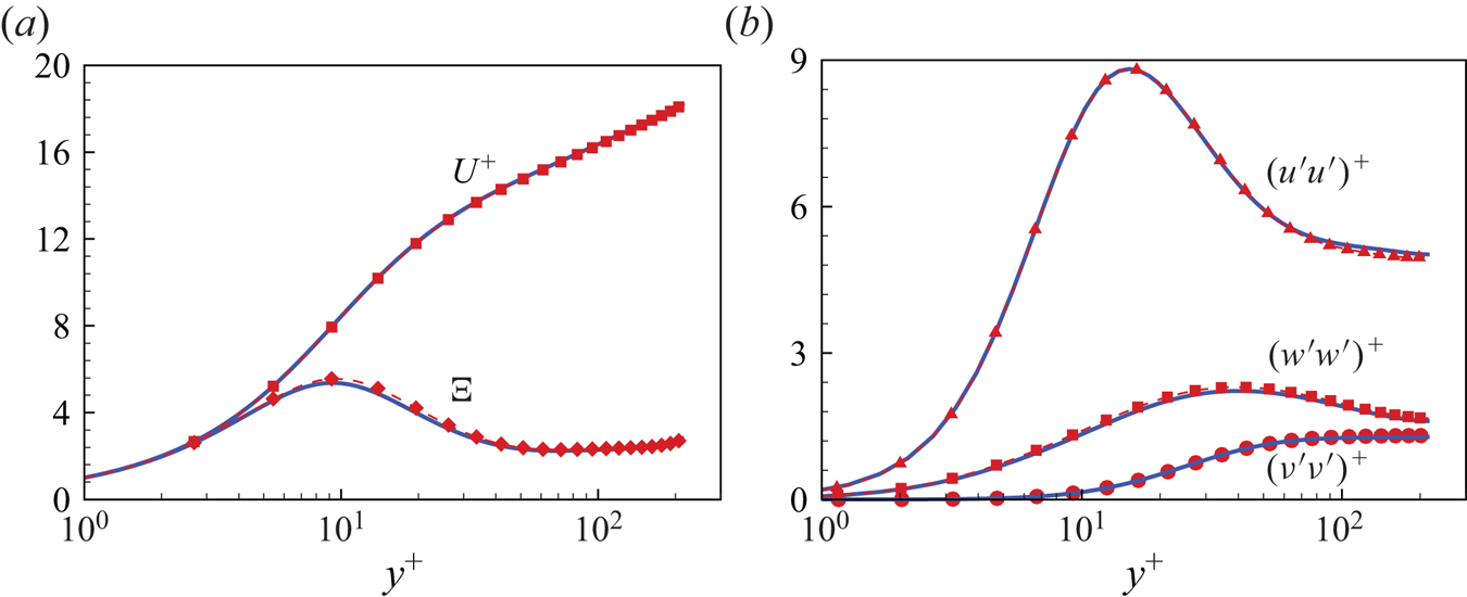
Figure 2 shows DNS verification at  $Re_c=4400$, compared with DNS at the same
 $Re_c$ by Lee & Moser (Reference Lee and Moser2018). Streamwise mean-velocity
 $U^+$ and scaled velocity gradient
 $\varXi = y^+ \textrm {d}U^+/{\textrm {d} y}^+$ versus
 $y^+$ are shown in figure 2(a) and scaled turbulent intensities
 $(u'u')^+$,
 $(v'v')^+$ and
 $(w'w')^+$ are shown in figure 2(b). We find that the two DNS match reasonably well, notably on
 $\varXi$ which clearly shows an uptilt near the centreline. This tendency is characteristic of medium-Reynolds-number PC flows as described by Pirozzoli et al. (Reference Pirozzoli, Bernardini and Orlandi2014).
Verification with DNS at  $Re_\tau \approx 220$. (a) Mean velocity profile
 $U^+$ and scaled velocity gradient
 $\varXi$. (b) Turbulence intensities
 $(u'u')^+$,
 $(v'v')^+$ and
 $(w'w')^+$. Lines, data from Lee & Moser (Reference Lee and Moser2018). Lines with symbols, present DNS results.

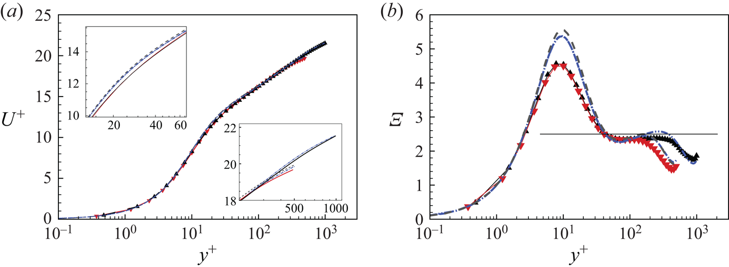
Beyond DNS, we compare in figure 3 our LES at  $Re_\tau \approx 500$ and
 $1000$ with the DNS data from Pirozzoli et al. (Reference Pirozzoli, Bernardini and Orlandi2014). DNS data at
 $Re_\tau =502.6$ from Lee & Moser (Reference Lee and Moser2018) are also included. Figure 3(a) shows streamwise velocity profiles of
 $U^+$ versus
 $y^+$. The LES generally agrees with DNS at both
 $Re_\tau$ values. For
 $y^+\sim Re_\tau$ with
 $Re_\tau \approx 500$, differences between our LES and the two DNS are similar to the differences between the two reference DNS results. At
 $Re_\tau \approx 1000$, our LES matches DNS data (Pirozzoli et al. Reference Pirozzoli, Bernardini and Orlandi2014), especially near the centreline as shown in the lower-right close-up inset. Near
 $y^+$ around
 $20\sim 40$, a small but systematic difference is apparent between DNS and LES, as shown in the upper-left close-up inset. This can be ascribed to the SGS model effect on the basic mean velocity for PC flow. The wall-normal averaged Navier–Stokes equations for statistically stationary PC flow show that
 $\textrm {d} U^+/ {\textrm {d} y}^+ - (u'v')^+ = 1$. In LES, the SGS model contributes to a part of
 $(u'v')^+$ and so directly influences the gradient of the mean velocity. This effect can be found in a plot of
 $\varXi$ in figure 3(b), where
 $\varXi$ from the LES is generally lower than that obtained by DNS at around
 $y^+ = 10$. In other regions of the
 $\varXi$ profile, the WRLES follows the trend of the corresponding reference DNS fairly well.
Verification of LES at  $Re_\tau \approx 500$ and
 $1000$. (a) Velocity profiles
 $U^+$. (b) Scaled velocity gradient
 $\varXi$. Dashed, DNS of Lee & Moser (Reference Lee and Moser2018). Dash–dotted and dash–double dotted, DNS of Pirozzoli et al. (Reference Pirozzoli, Bernardini and Orlandi2014). Line with
 $\blacktriangledown$ (red), LES of
 $Re_\tau = 500$. Line with
 $\blacktriangle$, LES of
 $Re_\tau = 1000$.

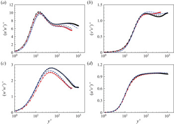
Figure 4 shows a comparison of the three diagonal and one off-diagonal components of the Reynolds stresses with DNS. All three turbulent intensities between two cases show satisfactory agreement. The behaviour of  $(u'v')^+$ agrees with the DNS data, starting from zero and increasing asymptotically to unity in the velocity-log region.
Comparison of LES with DNS at  $Re_\tau \approx 500$ and
 $1000$: (a)
 $(u'u')^+$; (b)
 $(v'v')^+$; (c)
 $(w'w')^+$; (d)
 $(u'v')^+$. For the key, see figure 3.

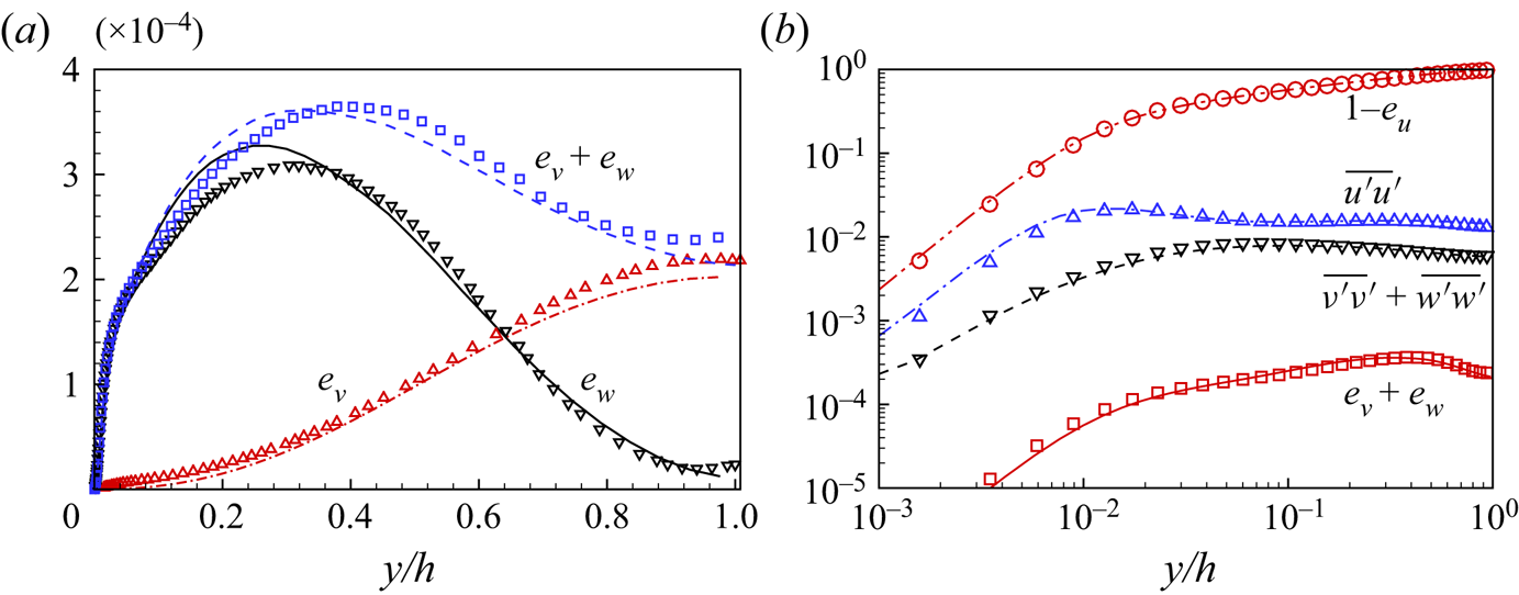
A kinetic-energy diagnostic can be defined for a velocity component  $\phi$ by
 \begin{equation} e_\phi (y) = \frac{1}{N_z} \sum_{z} \left( \frac{ \tilde{\phi}(y,z) }{U_c} \right) ^2 \end{equation}
leading to  $e_u(y)$,
 $e_v(y)$ and
 $e_w(y)$, which are energy densities in the wall-normal direction per unit span, scaled using the moving-wall velocity
 $U_c$. Both
 $e_v$ and
 $e_w$ are measures of the roll energy magnitude. We compare wall-normal profiles of
 $e_v$ and
 $e_w$ from the WRLES with DNS data (Pirozzoli et al. Reference Pirozzoli, Bernardini and Orlandi2014). In figure 5(a), both
 $e_v$ and
 $e_w$ scaled on
 $U_c^2$ show similar trends to DNS data with maximum discrepancy near the centreline for
 $e_v$ of approximately
 $10\,\%$. We also plot
 $e_v + e_w$, which can be interpreted as a measure of the energy of the rolls that exhibit structured fluid motion in the plane perpendicular to the streamwise direction. Figure 5(b) shows profiles of the four different quantities for WRLES and DNS. At the flow centreline, the turbulence intensities are approximately
 $1\,\%$ of
 $U_c^2$, while the roll energy,
 $e_v+e_w$, is approximately
 $0.01\,\%$ of
 $U_c^2$. The WRLES represented by lines agrees quite well with the reference DNS data, which demonstrates its capability of capturing subtle physical properties of the spanwise rolls.
Verification of roll energy at  $Re_\tau \approx 1000$. (a) Roll kinetic energy components
 $e_v$,
 $e_w$. (b) Comparison of four quantities:
 $e_u$,
 $(u'u')^+$,
 $(v'v')^+ +(w'w')^+$ and
 $e_v+e_w$. Lines, present LES results; symbols, reference DNS by Pirozzoli et al. (Reference Pirozzoli, Bernardini and Orlandi2014).

4. Wall-resolved LES: up to  $Re_\tau \approx 3600$

4.1. Velocity profiles
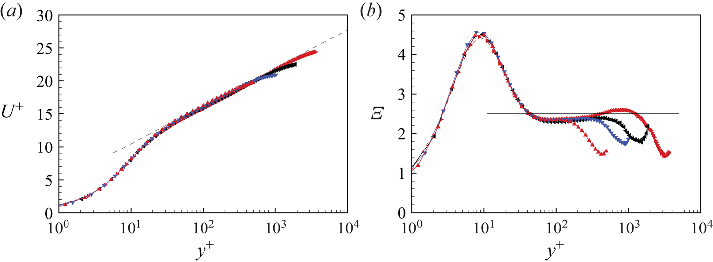
Figure 6(a) shows the scaled streamwise velocity  $U^+$ of four WRLES. Also plotted is a log law
 $U^+ = \ln (y^+)/\kappa + B$ with
 $\kappa = 0.4$ and
 $A=5.0$. The WRLES shows a consistent log-region across the
 $Re_c$ range. This is also observed in the
 $\varXi -y^+$ plot of figure 6(b).
Mean velocity profile of wall-resolved LES data. (a) Velocity profiles  $U^+$. (b) Scaled velocity gradient
 $\varXi$. Here,
 $\blacktriangle$ (red),
 $Re_\tau \approx 500$;
 $\blacktriangledown$ (blue),
 $Re_\tau \approx 1000$;
 $\blacktriangleleft$,
 $Re_\tau \approx 1800$;
 $\blacktriangleright$ (red),
 $Re_\tau \approx 3600$.

4.2. Fluctuations
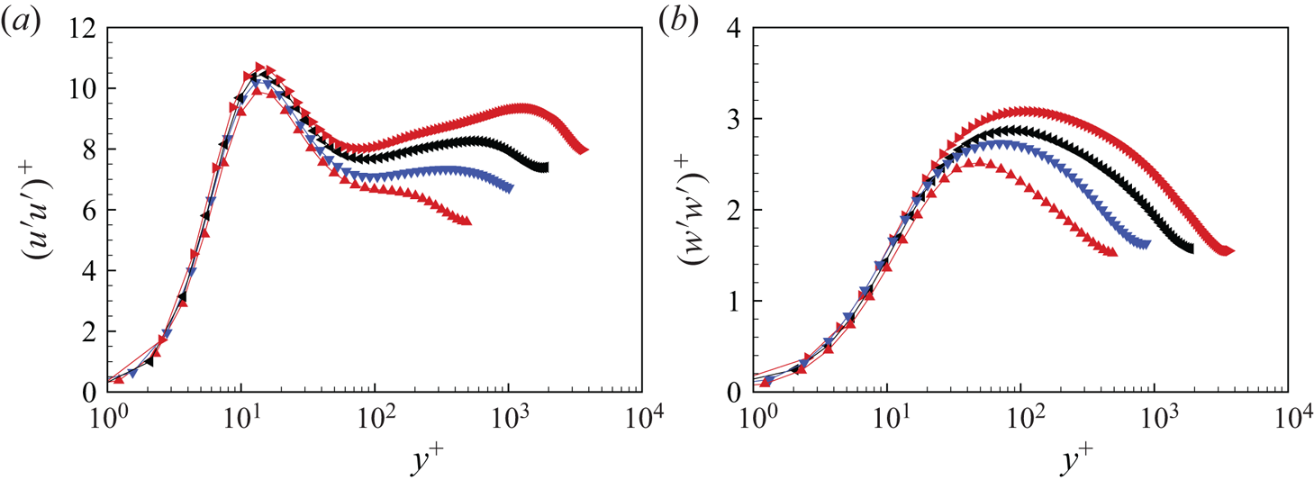
Figure 7 shows the averaged Reynolds stress  $(u'u')^+$ and
 $(w'w')^+$ in inner scaling. The four WRLES up to
 $Re_\tau \approx 3,600$ show consistent trends. The inner scaling of the two intensities show a lack of universality in the general shape, in agreement with the observation of Pirozzoli et al. (Reference Pirozzoli, Bernardini and Orlandi2014). The wall-normal position of the first peak, at
 $y^+ \approx 15$ for all cases, is in general agreement with other canonical flows including channel flow data by Lee & Moser (Reference Lee and Moser2015), pipe flow data by Willert et al. (Reference Willert, Soria, Stanislas, Klinner, Amili, Eisfelder, Cuvier, Bellani, Fiorini and Talamelli2017) and also Taylor–Couette flow (Ostilla-Mónico et al. Reference Ostilla-Mónico, Verzicco, Grossmann and Lohse2016; Cheng, Pullin & Samtaney Reference Cheng, Pullin and Samtaney2020). Pirozzoli et al. (Reference Pirozzoli, Bernardini and Orlandi2014) emphasize the presence of a secondary peak in
 $(u'u')^+$ at
 $y/h\approx 0.33$ in DNS-PC data at
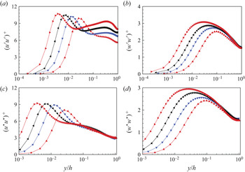
 $Re_\tau \approx 1000$. For WRLES, this secondary peak is presently observed at similar locations for all higher
 $Re_\tau$ flows, as shown in figure 8(a,b) for outer scaling plots of
 $(u'u')^+$ and
 $(w'w')^+$. For PC flow, this secondary peak clearly emerges at
 $Re_\tau \approx 1000$, which is similar to the range of
 $Re_\tau \approx 2000$ found in Taylor–Couette flow (Ostilla-Mónico et al. Reference Ostilla-Mónico, Verzicco, Grossmann and Lohse2016). These
 $Re_\tau$ values are generally much smaller than those observed for the first appearance of a secondary peak in canonical flows, for example
 $Re_\tau =19\,918$ in the pipe flow experiments by Willert et al. (Reference Willert, Soria, Stanislas, Klinner, Amili, Eisfelder, Cuvier, Bellani, Fiorini and Talamelli2017). A plausible hypothesis is that the secondary peak in Couette flow is probably related to the existence of large-scale rolls which effectively enhance the turbulent mixing and thus the energy transport.
Turbulent intensities in inner scale  $y^+$ for wall-resolved LES cases: (a)
 $(u'u')^+$; (b)
 $(w'w')^+$. Here,
 $\blacktriangle$ (red),
 $Re_\tau \approx 500$;
 $\blacktriangledown$ (blue),
 $Re_\tau \approx 1000$;
 $\blacktriangleleft$,
 $Re_\tau \approx 1800$;
 $\blacktriangleright$ (red),
 $Re_\tau \approx 3600$.

Turbulent intensities in outer scaling  $y/h$ for wall-resolved LES: (a)
 $(u'u')^+$; (b)
 $(w'w')^+$; (c)
 $(u^\bullet u^\bullet )^+$; (d)
 $(w^\bullet w^\bullet )^+$. Here,
 $\blacktriangle$ (red),
 $Re_\tau \approx 500$;
 $\blacktriangledown$ (blue),
 $Re_\tau \approx 1000$;
 $\blacktriangleleft$,
 $Re_\tau \approx 1800$;
 $\blacktriangleright$ (red),
 $Re_\tau \approx 3600$.

To understand fluctuations generated by the small-scale turbulence only, we plot  $\overline {u^\bullet u^\bullet }$ in the form
 $(u^\bullet u^\bullet )^+$ in figure 8(c) and
 $(w^\bullet w^\bullet )^+$ in figure 8(d). Figure 5(b) indicates that for the spanwise component,
 $e_w \approx 1\,\%\, \overline {w'w'}$. Because
 $\overline {w^\bullet w^\bullet } = \overline {w'w'} - e_w$, it is clear that wall-normal profiles of
 $\overline {w^\bullet w^\bullet }$ will be similar to those for
 $\overline {w'w'}$, in both inner and outer scaling. In contrast, the streamwise rolls do impose a strong imprint on streamwise turbulent intensities. The profiles of
 $(u^\bullet u^\bullet )^+$ are generally rather smaller in magnitude than
 $(u'u')^+$ and do not show a monotonic increasing tendency at fixed
 $y/h$ with increasing
 $Re_\tau$ in the outer flow region.
5. Wall-resolved LES: spanwise variation
Here we analyse the spanwise variation of the mean velocity and turbulent intensities produced by the streamwise rolls.
5.1. Effect of spanwise variation: $Re_\tau \approx 500$

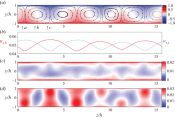
In figure 9, we show the averaged flow field in the  $y\text {--}z$ plane. Colour-coded contours of the streamwise velocity
 $\tilde {u}$ in figure 9(a), with mean
 $(y\text {--}z)$-plane streamlines added to show the averaged circulatory motion within rolls, clearly indicate a strong spanwise variation associated with roll motion. Figure 9(b) shows the variation of the local skin-friction velocity along the spanwise
 $z$ direction. We define local skin-friction velocities
 $u_{\tau,b}(z)$ and
 $u_{\tau,t}(z)$ on the bottom and top walls respectively as
 $u_{\tau,b}^2 = | \textrm {d} \tilde {u} / {\textrm {d}y}|_{y=-h}$ and
 $u_{\tau,t}^2 = | \textrm {d} \tilde {u} / {\textrm {d} y}|_{y=h}$. Both
 $u_{\tau,b}(z)$ and
 $u_{\tau,t}(z)$ show a wavy variation in
 $z$ produced by the cross-stream velocity field of the rolls. We remark that there may also exist a spanwise component of the skin-friction vector at the wall, which leads to an effective spanwise
 $u_{\tau }$, but this is small and is neglected.
Span-wise variation of PC flow,  $Re_\tau \approx 500$ (a) Contours of
 $\tilde {u}$ with streamlines of the mean cross-flow
 $(\tilde {v}-\tilde {w})$ velocity field. (b) Local skin-friction velocity: red,
 $u_{\tau,b}$ and dashed,
 $u_{\tau,t}$. (c) Contours of
 $\widetilde {u^\bullet u^\bullet }$. (d) Contours of
 $\widetilde {u' u'}$.

In the plots of  $\widetilde {(u^\bullet u^\bullet )}$ in figure 9(c), we observe six regions in the domain shown, illustrated as near-white zones, which depict minimum values. Each region denotes momentum transport induced by a quite strong vertical flow. For example, at position ‘a’ of figure 9(a), a strong vertical flow from bottom to top corresponds to the minimum region of
 $\widetilde {(u^\bullet u^\bullet )}$ near the bottom wall at the same position in figure 9(c). Similarly, at position ‘c’, a strong vertical flow from top to bottom corresponds to the minimum region of
 $\widetilde {(u^\bullet u^\bullet )}$ near the top wall at the same position. Owing to the different averaging methods, there exist other possible diagnostics, for example
 $\widetilde {(u' u')}$, as plotted in figure 9(d). Because this does not generally exhibit any interesting structures, this is noted but not discussed subsequently.
5.2. Scaling of $\tilde {u}$ and $\widetilde {u^\bullet u^\bullet }$ at $Re_\tau \approx 500$


We examine the local velocity profiles at specific spanwise locations, for example, at three locations ‘ $a$’, ‘
 $b$’ and ‘
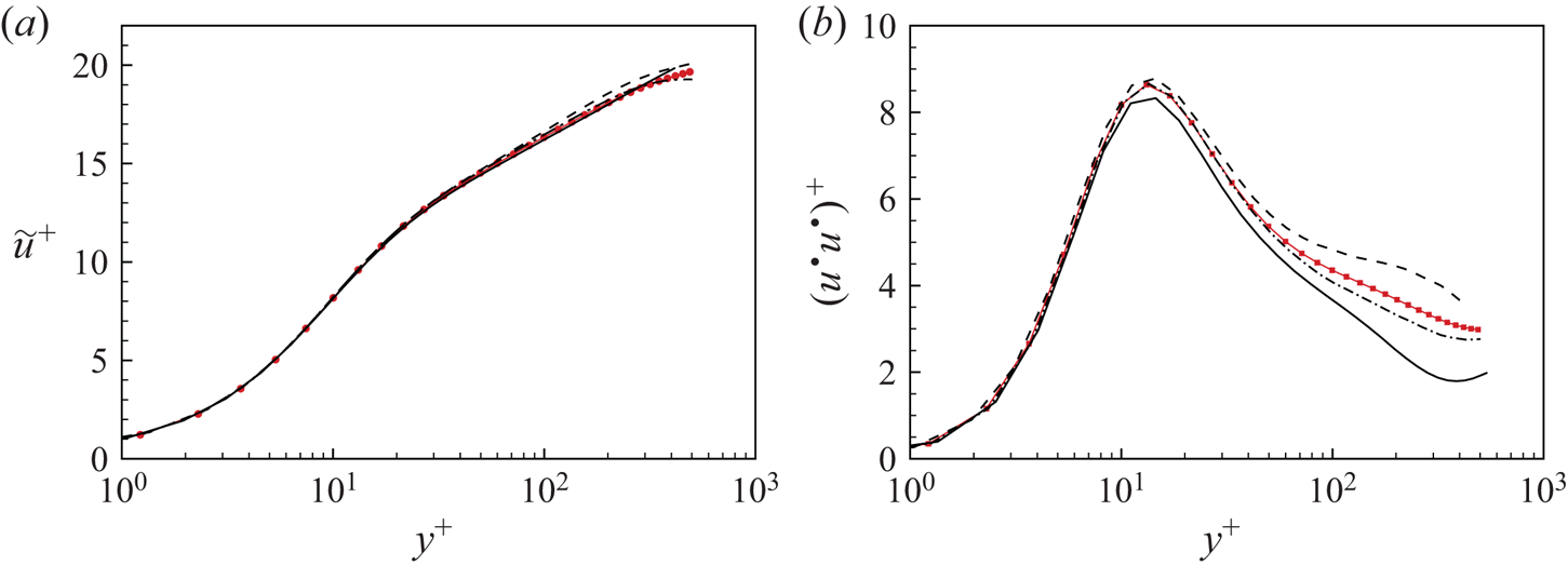
 $c$’ as labelled in figure 9. In figure 10, we plot the scaled streamwise velocity profiles
 $\tilde {u}^+ = \tilde {u}/u_{\tau,b}$ and related turbulence intensities
 $\widetilde {u^\bullet u^\bullet }^+ = \widetilde {u^\bullet u^\bullet }/u^2_{\tau,b}$. When scaled using local skin-friction velocity, streamwise profiles at different locations show similar log-like variation, not much removed from the scaled mean flow
 $U^+$ which is also plotted. The behaviour of turbulence intensities is different. In near-wall regions, say
 $y^+<50$, turbulence intensities show similar behaviour to span-wise averaged intensities, while for regions near the centreline, the differences between turbulence intensities at different spanwise locations are substantial, and imply turbulence momentum transport by the spanwise circulatory flow.
Comparisons at selected locations ‘ $a$’, ‘
 $b$’ and ‘
 $c$’,
 $Re_\tau \approx 500$: (a) Streamwise velocity
 $\tilde {u}$; (b) turbulent intensities
 $(u^\bullet u^\bullet )^+$ dashed line, location ‘
 $a$’; dash–dotted line, location ‘
 $b$’; solid line, location ‘
 $c$’. Line with filled symbols,
 $U^+$ in panel (a) and
 $(u'u')^+$ in panel (b).

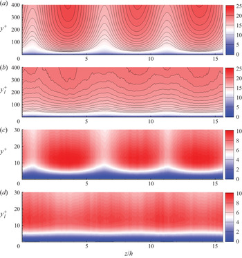
To give a full picture of velocity scaling, it is useful to examine a two-dimensional  $y\text {--}z$ plane contour plot of the scaled streamwise velocity. We focus on the velocity near the bottom wall which is chosen as the reference coordinate. In figure 11, we show plots with different scalings. The spanwise coordinate is scaled as
 $z/h$. Figure 11(a) shows
 $U^+$ with normal distance using
 $y^+$. The spanwise velocity variation is apparent because this scaling uses the global
 $u_\tau$. In figure 11(b), both
 $\tilde {u}$ and
 $y$ are scaled using the local
 $u_{\tau,b}(z/h)$. Here we define
 $y_l^+(y,z) = y u_{\tau,b}/\nu$. Using the local
 $u_{\tau,b}$, the spanwise velocity variation is mostly flattened.
Scaling of velocity component  $\tilde {u}$ and streamwise turbulent intensities
 $\widetilde {u^\bullet u^\bullet }$,
 $Re_\tau \approx 500$: (a)
 $\tilde {u}/u_\tau$ in the
 $(y^+, z/h)$ plane; (b)
 $\tilde {u}/u_{\tau,b}$ in the
 $(y_l^+, z/h)$ plane; (c)
 $\widetilde {u^\bullet u^\bullet }/u^2_\tau$ in the (
 $y^+,z/h$) plane; (d)
 $\widetilde {u^\bullet u^\bullet }/u^2_{\tau,b}$ in the (
 $y_l^+,z/h$) plane. Here
 $y_l^+ = y u_{\tau,b}/\nu$.

For the scaling of streamwise turbulence intensities, we focus on the near-wall region in  $y_l^+ < 30$. We compare two scalings, one is using
 $u_\tau$ in figure 11(c), the second using
 $u_{\tau,b}$ in figure 11(d), for both turbulence intensity and distance. Again, using local
 $u_{\tau,b}$ removes much but not all of the
 $z/h$ variation.
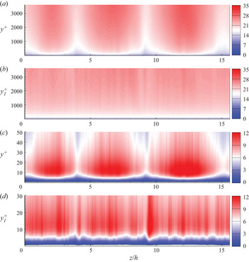
5.3. Scaling of $\tilde {u}$ and $\widetilde {u^\bullet u^\bullet }$ at $Re_\tau \approx 3600$


We repeat this scaling of  $\tilde {u}$ and
 $\widetilde {u^\bullet u^\bullet }$ for higher Reynolds number flow. In figure 12(a,b), we show two plots, one is
 $\tilde {u}/u_\tau$ in the (
 $y^+,z/h$) plane and the other is
 $\tilde {u}/u_{\tau,b}$ in the (
 $y_l^+,z/h$) plane. Again, using local scaling
 $u_{\tau,b}$ does show a flattened variation in the spanwise direction.
Scaling of streamwise velocity  $\tilde {u}$ and streamwise turbulence intensities
 $\widetilde {u^\bullet u^\bullet }$,
 $Re_\tau \approx 3600$: (a)
 $\tilde {u}/u_\tau$ in the (
 $y^+,z/h$) plane; (b)
 $\tilde {u}/u_{\tau,b}$ in the (
 $y_l^+,z/h$) plane; (c)
 $\widetilde {u^\bullet u^\bullet }/u^2_\tau$ in the (
 $y^+,z/h$) plane; (d)
 $\widetilde {u^\bullet u^\bullet }/u^2_{\tau,b}$ in the (
 $y_l^+,z/h$) plane.

In figure 12(c,d), we again focus on the bottom near-wall region and display the scaling effect using the local  $u_{\tau,b}(z/h)$. Compared with using
 $u_\tau$, which clearly shows the roll effect, employing
 $u_{\tau,b}$ smooths the effect of the large-scale roll structure. Using
 $u_{\tau,b}(z/h)$ does show the presence of small-scale spanwise fluctuations. We expect these to be even smoother using longer timewise averaging.
We also discuss scaled profiles at a specific spanwise location. In figure 13, we show the scaled streamwise velocity profiles  $\tilde {u}^+$ and related turbulence intensities
 $\widetilde {u^\bullet u^\bullet }^+$. Streamwise mean-velocity profiles at different spanwise locations show a log-like region when scaled on the local skin-friction velocity. The behaviour of turbulence intensities is similar to the results at
 $Re_\tau \approx 500$. In the near-wall region, inner scaling using
 $u_\tau$ gives reasonable collapse, while outer-region structures are generally substantially different. The presence, in PC flow, of spanwise local inner scaling including a near-wall log layer in the mean-velocity profile is consistent with the present wall model, as described in § 2.3, which uses both of these features.
Comparisons at selected locations ‘ $a$’, ‘
 $b$’ and ‘
 $c$’,
 $Re_\tau \approx 3600$: (a) streamwise velocity
 $\tilde {u}$; (b) turbulence intensities
 $(u^\bullet u^\bullet )^+$. Symbols are the same as in figure 10.

6. Wall-modelled LES with $Re_\tau =3.6\times 10^3\text {--}2.8 \times 10^{5}$

Wall-modelled LES provides a method for extending the simulations to  $Re_c$ that are outside the range of WRLES with the present computational resources. Wall-modelled LES enables this but at the cost that both near-wall and small-scale processes over the whole domain are modelled and not resolved. While this limits utility, WMLES can nonetheless provide useful scaling information provided that the wall-model can recognize subtle Reynolds number effects. Our strategy is to first overlap the WMLES with WRLES at
 $Re_\tau \approx 3600$. While this does not provide ground-truth verification, it can give confidence in continuing the WMLES to higher
 $Re_\tau$.
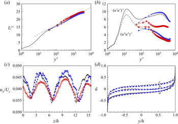
In figure 14, we compare some one-point diagnostics for WRLES and WMLES at  $Re_\tau \approx 3600$. Figure 14(a) shows the inner-scaled mean velocity
 $U^+$ for both coarse-mesh and fine-mesh WMLES. The respective resolutions are shown in table 2. Both generally match the WRLES mean-velocity profile fairly well. Using a coarse mesh, the near-wall effect can be seen in the form of somewhat lifted velocity profiles, while the finer-mesh with
 $\Delta x^+ = \Delta y^+ = \Delta z^+$ shows a smaller wall-point effect.
Wall-modelled LES at  $Re_\tau \approx 3600$. (a) Scaled velocity profile
 $U^+$. Dashed line, log law with
 $U^+ = \ln y^+/0.4 + 5.0$. (b) Streamwise turbulence intensities
 $(u'u')^+$ and
 $(u^\bullet u^\bullet )^+$. (c) Skin-friction velocity
 $u_{\tau }$. (d) Velocity profile
 $\tilde {u}$ at specific locations ‘
 $a$’, ‘
 $b$’ and ‘
 $c$’. For locations, see figure 9(a). Lines, data from wall-resolved LES; lines with hollow symbols, coarse-mesh WMLES; line with filled symbols, fine-mesh WMLES. See table 2.

Figure 14(b) compares the streamwise turbulence intensities, which include  $(u'u')^+$ and
 $(u^\bullet u^\bullet )^+$. The fine-mesh WMLES generally captures the trends of both WRLES intensities, while the coarse-mesh simulation shows strong deviations, especially for
 $(u'u')^+$. The reason for requiring higher-than-expected spanwise resolution is almost certainly related to spanwise inhomogeneity produced by the presence of the rolls. This creates a three-dimensional mean flow that drives the spanwise inhomogeneous turbulence fluctuations. Additionally, the rolls result in quite complex turbulence separation/reattachment events within individual roll pairs at each wall surface. Accurately capturing these features in WMLES appears to require higher resolution than for a Poiseuille-channel flow at similar
 $Re_\tau$.
The present meshes used for WRLES and WMLES are consistent with those of Choi & Moin (Reference Choi and Moin2012) although a relatively fine spanwise mesh is required to capture streamwise-roll structures. For  $Re_c \approx 10^5$, the WMLES mesh is comparable to that for WRLES, while a WRLES at
 $Re_c \approx 10^7$ would result in a difference of two to three orders of magnitude.
In figure 14(c), we show the  $u_{\tau }(z/h)$ variation in the spanwise direction while figure 14(d) shows the mean streamwise velocity profile across the channel at three specific spanwise locations defined in figure 9(a). Again, the fine-mesh WMLES reproduces the wall-resolved LES results in the bulk flow region.
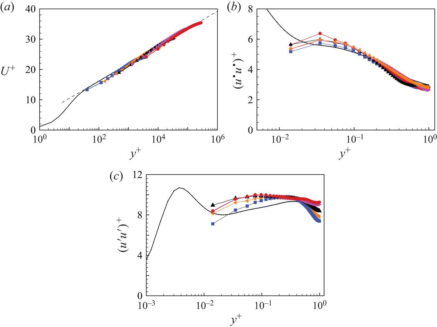
The mean streamwise velocity profiles for all WMLES are shown in figure 15(a). Also shown is a log relationship with  $\kappa = 0.4$ and
 $A=5.0$. All profiles appear to capture the log region reasonably well. The streamwise turbulence intensity component
 $(u^\bullet u^\bullet )^+$ shows collapse over much of the flow domain in figure 15(b). Figure 15(c) shows the WMLES results for
 $(u' u')^+$ against the WRLES results at
 $Re_\tau = 3600$. The present high-
 $Re_\tau$ WMLES does not show the presence of a secondary peak whose magnitude increases with increasing
 $Re_\tau$. It was shown earlier that a quite fine spanwise resolution was required to capture the
 $(u' u')^+$ profile at
 $Re_\tau = 3600$. It is certainly possible that an increasingly fine resolution with increasing
 $Re_\tau$ beyond
 $3600$ is required to capture possible further increases in the magnitude of the secondary peak. However, figure 15(c) could be interpreted as suggesting the formation of an asymptotic plateau in
 $(u' u')^+$ when
 $Re_\tau \rightarrow \infty$ that joins the first and second peaks with no further increase with increasing
 $Re_\tau$. Further research will be required to resolve this issue.
Wall-modelled LES at different  $Re_\tau$: (a) mean velocity profiles; (b) streamwise turbulence intensities
 $(u^\bullet u^\bullet )^+$; (c) streamwise turbulence intensities
 $(u' u')^+$. Line, WRLES at
 $Re_\tau \approx 3600$;
 $\square$ (blue),
 $Re_\tau \approx 3600$;
 $\blacktriangleleft$ (orange),
 $Re_\tau \approx 1.1\times 10^4$;
 $\blacktriangle$,
 $Re_\tau \approx 3.3\times 10^4$;
 $\blacktriangleright$ (pink),
 $Re_\tau \approx 9.1\times 10^4$;
 $\bullet$ (red),
 $Re_\tau \approx 2.8\times 10^5$. Dashed line in panel (a), log law of
 $U^+ = \ln y^+/0.4 + 5.0$.

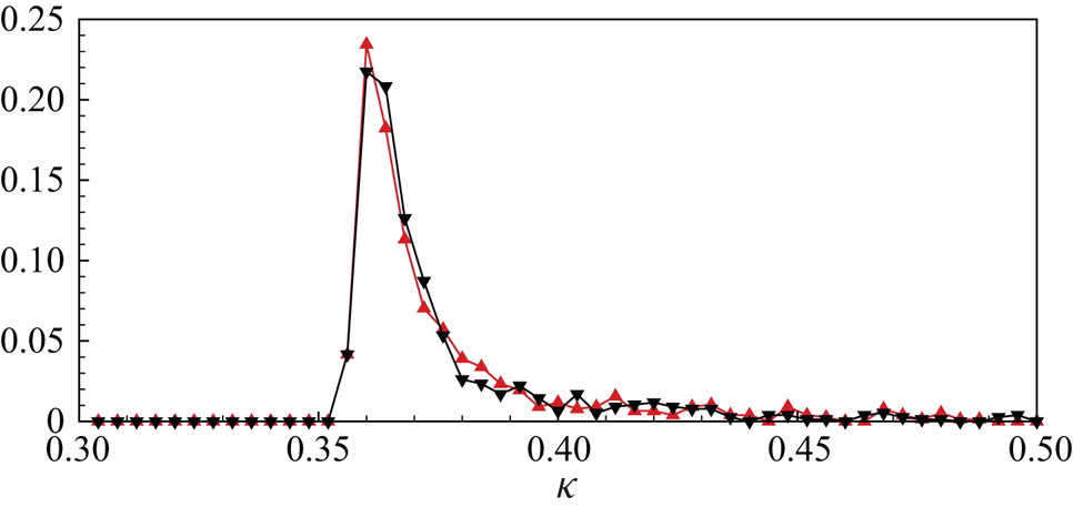
It is of interest to document the distribution of the local virtual-wall-model Kármán constant, as dynamically computed from the ODE in WMLES; see (2.5a,b). Its probability density function (p.d.f.) is shown in figure 16 for two Reynolds numbers,  $Re_c= 9\times 10^4$ and
 $10^7$. Both p.d.f.s show a peak and a long tail. Although the peak value is around
 $\kappa =0.37$, the average value is in the range 0.4–0.41, consistent with both accepted values for general canonical wall-bounded flows and values for the present PC-flow mean velocity profiles. This demonstrates approximate continuity between the virtual-wall model and the calculated WMLES mean velocity profiles.
Probability density function of the instantaneous, calculated Kármán constant  $\kappa$. Here,
 $\blacktriangle$ (red),
 $Re_\tau \approx 3600$;
 $\blacktriangledown$,
 $Re_\tau \approx 2.8\times 10^5$.

7. Skin-friction relation
7.1. Skin-friction relation and the centreline, mean-velocity gradient
The asymptotic behaviour of the mean-velocity gradient, both near the wall and at the centreline, is the key feature of the wall-bounded Couette-flow turbulence. In a previous study of Taylor–Couette flow with the inner cylinder rotating, a three-zone model was established that used the existence of a constant-angular-momentum zone in the bulk of the flow (Cheng et al. Reference Cheng, Pullin and Samtaney2020). For a PC flow, a simpler approach is to obtain an  $Re_{\tau }\text {--}Re_c$ through a two-log match at the flow centreline (Pirozzoli et al. Reference Pirozzoli, Bernardini and Orlandi2014). Following their model by assuming the velocity profiles in the form of log laws without wakes, and with constants
 $\kappa$ and
 $A$, we have the following mean velocity profiles.
I:  $-h< y \leqslant 0$ with
 \begin{equation} U = U_c - u_{\tau}\left( \frac{1}{\kappa}\ln\left(\frac{( h + y )\,u_{\tau}}{\nu}\right) +A \right). \end{equation}
II:  $0 \le y < h$ with
 \begin{equation} U ={-}U_c + u_{\tau}\left( \frac{1}{\kappa}\ln\left(\frac{( h - y)\,u_{\tau}}{\nu}\right) +A \right).\end{equation}
Matching of these two profiles at the centreline  $y=0$ gives the following relation:
 \begin{equation} \frac{Re_c}{Re_{\tau}} = \frac{1}{\kappa} \ln Re_\tau + A, \end{equation}
which provides the skin-friction relation for PC flow. This equation can be solved for  $Re_\tau$ to give
 \begin{equation} Re_\tau = \frac{\kappa Re_c}{ W (\textrm{e}^{A\kappa} \kappa Re_c )}, \end{equation}
where  $W(Z)$ is the ProductLog function or Lambert function, which is the solution of
 $Z = W\ln (W)$. Plots of
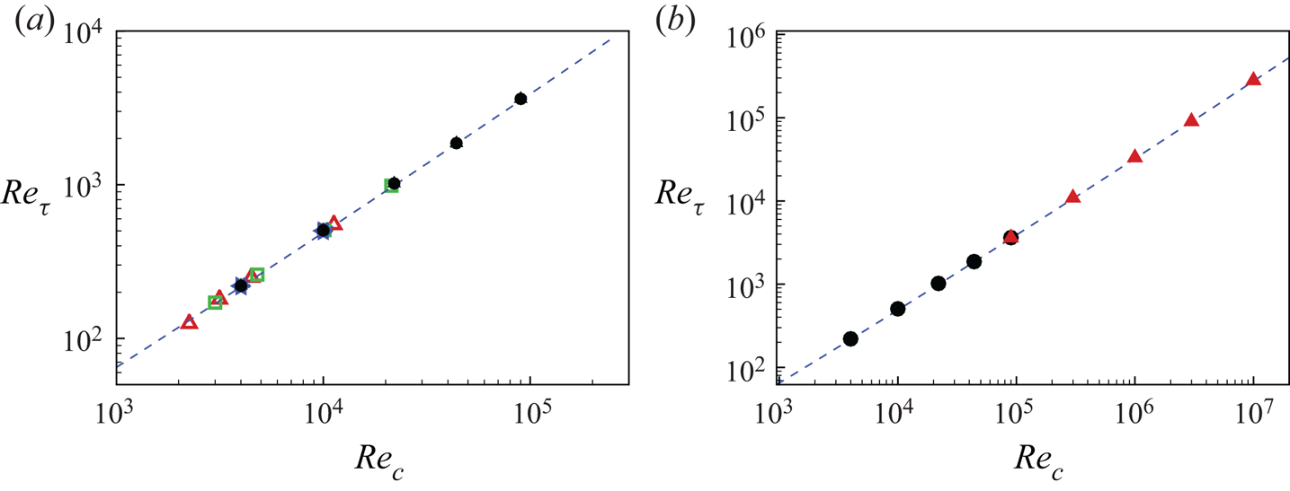
 $Re_{\tau }\text {--}Re_c$ are shown in figure 17, which includes existing DNS reference data and also the present WR and WMLES and (7.3). The constants
 $\kappa$ and
 $A$ are chosen using classical values
 $\kappa =0.4$ and
 $A=5.0$. For the
 $Re_{\tau }\text {--}Re_c$ relation, all available DNS data reasonably agree with the theoretical estimate. Our present LES results are plotted in figure 17(b). The wall-modelled LES reasonably follow the modelled equation in this
 $Re_c$ range.
Skin-friction relation  $Re_{\tau }\text {--}Re_c$: (a) wall-resolved LES data comparison with DNS; (b) all present LES results. Here,
 $\triangle$ (red), DNS by Avsarkisov et al. (Reference Avsarkisov, Hoyas, Oberlack and García-Galache2014);
 $\square$ (green), DNS by Pirozzoli et al. (Reference Pirozzoli, Bernardini and Orlandi2014);
 $\diamond$ (blue), DNS by Lee & Moser (Reference Lee and Moser2018);
 $\bullet$, wall-resolved LES;
 $\blacktriangle$ (red), wall-modelled LES. Dashed line (blue), (7.3) with
 $\kappa =0.4$ and
 $A=5.0$.

The model can be extended to calculate the mean-flow velocity gradient at the centreline. Because the above two velocity profiles also have a continuous velocity gradient at the centreline, we can obtain
 \begin{equation} S \equiv \frac{h}{U_c} \frac{\partial U}{\partial y} ={-} \frac{1}{\kappa } \frac{Re_\tau}{Re_c}. \end{equation}
Using (7.4) to eliminate  $Re_\tau$, we obtain
 \begin{equation} S = \frac{1}{ W (\textrm{e}^{A\kappa} \kappa Re_c ) }. \end{equation}
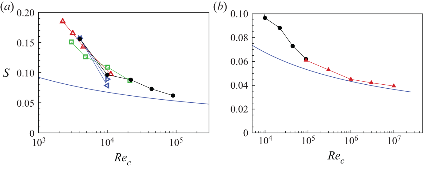
Plots of  $S(Re_c)$ are given in figure 18. Lower
 $Re_c$ cases, which include existing DNS reference data and the present WRLES results, are also shown in figure 18(a). The theory generally underestimates the numerical data for relatively low Reynolds number but our largest
 $Re_c$ WRLES data, at
 $Re_\tau \approx 3600$, reasonably matches the model estimate. Figure 18(b) shows a higher
 $Re_c$ comparison where agreement between theory and the WMLES is acceptable.
Scaled velocity gradient at centreline,  $S$. (a) Wall-resolved LES data comparison with DNS. (b) All present LES results. Here,
 $\triangle$ (red), DNS by Avsarkisov et al. (Reference Avsarkisov, Hoyas, Oberlack and García-Galache2014);
 $\square$ (green), DNS by Pirozzoli et al. (Reference Pirozzoli, Bernardini and Orlandi2014);
 $\triangleleft$ (blue), short domain DNS by Lee & Moser (Reference Lee and Moser2018);
 $\triangleright$ (blue), long domain DNS by Lee & Moser (Reference Lee and Moser2018);
 $\bullet$, wall-resolved LES;
 $\blacktriangle$ (red), wall-modelled LES. Line (blue), (7.6) with
 $\kappa =0.4$ and
 $A=5.0$.

7.2. Large $Re_\tau$ limit for streamwise mean flow velocity

Using (7.2) and (7.3) gives, for  $0 \le y < h$,
 \begin{equation} \frac{U(y)}{U_c} = \frac{ \ln \left(1-\dfrac{y}{h} \right) }{ \ln Re_\tau + \kappa A }. \end{equation}
According to the model, when  $Re_\tau \to \infty$ at any finite
 $y/h$, then
 $U(y)/U_c\to 0$, while from (7.6),
 $S\to 0$. This will not extend to the upper wall
 $y\to h$ where a thin viscous-dominated layer can be expected to remain at any
 $Re_\tau$. The velocity in the lower-half domain will show similar behaviour.
7.3. Spanwise skin-friction variation
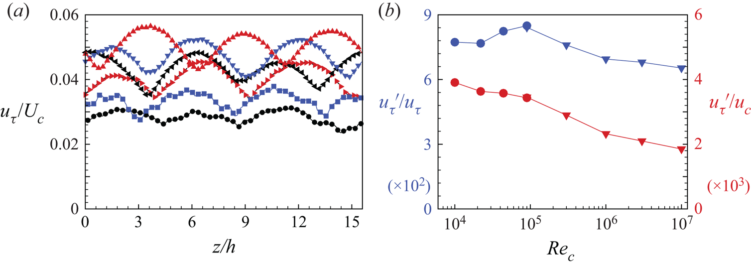
In figure 19(a), we show the spanwise variation of the skin-friction velocity  $u_{\tau }(z/h)/U_c$ at different
 $Re_\tau$. The periodic-like variation corresponds to the presence of spanwise rolls. It can be seen that, in addition to the decrease of the spanwise mean with increasing
 $Re_\tau$, the amplitude of the spanwise variation also decreases. Figure 19(b) shows the spanwise root-mean-squared variation
 $u'_\tau$ versus
 $Re_\tau$. When
 $u'_\tau$ is scaled using
 $U_c$, it generally shows a monotonic decreasing tendency. The plot of
 $u'_\tau /u _\tau$ shows an initial increase with increasing
 $Re_\tau$ followed by a slow decline.
Spanwise variation of skin-friction velocity. (a) Comparison of  $u_{\tau }$ at different
 $Re_c$. Here,
 $\blacktriangle$ (red),
 $Re_\tau \approx 500$;
 $\blacktriangledown$ (blue),
 $Re_\tau \approx 1000$;
 $\blacktriangleleft$,
 $Re_\tau \approx 1800$;
 $\blacktriangleright$ (red),
 $Re_\tau \approx 3600$;
 $\blacksquare$ (blue),
 $Re_\tau \approx 3.3\times 10^4$;
 $\bullet$,
 $Re_\tau \approx 2.8\times 10^5$. (b) Measure of root mean square of
 $u_{\tau }$:
 $u'_\tau / u_\tau$ and
 $u'_\tau / U_c$.

8. Roll behaviour
Spanwise rolls are generally observed in turbulent PC flows. While the rolls strengthen in magnitude during laminar to turbulent transition, there is little documentation in the literature concerning high-  $Re_c$ behaviour.
8.1. Instantaneous velocity fields
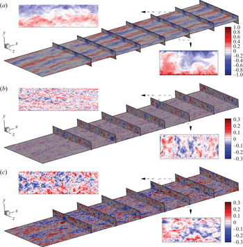
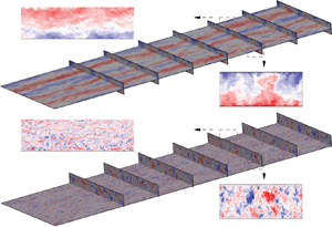
Visualization of component velocity fields provides insight into large-scale, steamwise roll behaviour. In figure 20, we show velocity contours on several two-dimensional planes in a front (streamwise)-top (wall-normal) view of the three-dimensional flow. The planes shown include one wall-parallel plane and seven cross-flow planes. These cross-flow planes are located at intervals of  $L_x/8$. For a better view of the inflow, planes at inflow and
 $L_x/8$ are hidden. In each figure, we also show two close-up frames to observe detailed flow features. One is from the cross-flow plane at
 $x=3L_x/4$, while the other on the wall-parallel plane starting at
 $x= 3L_x/4$.
Instantaneous velocity fields,  $Re_\tau \approx 500$: (a) streamwise velocity u; (b) vertical velocity
 $v$; (c) spanwise velocity
 $w$.

Figure 20(a) shows a colour-coded image of the streamwise velocity  $u$ on the wall-parallel plane
 $y=0$. The mean velocity is zero allowing clear observation of roll structures. In figures 20(b) and 20(c), where the wall-normal and span-wise velocities
 $v,w$, respectively, are shown, the parallel plane at
 $y=0.85h$ is chosen to enable clear visualization of both cross-flow and wall-parallel flow features. Instantaneous roll signatures are more apparent in the
 $u$-velocity image, including both the three pair rolls on the wall-parallel plane and their intrusion flow counterparts into opposite walls on cross-flow planes. In plots of
 $v$ and
 $w$, detectable flow structures seem relatively small and large-scale rolls are hard to discern. An interesting feature is that the near-wall flow structure is clearly smaller than that in the flow within the bulk region, especially in the
 $v$ and
 $w$ images.
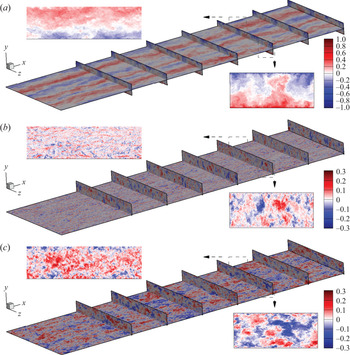
To show  $Re_\tau$ effects, similar images of
 $u$,
 $v$ and
 $w$ WRLES at
 $Re_\tau \approx 3600$ are plotted in figure 21. Compared with
 $Re_\tau \approx 500$, the
 $u$-visualization shows little apparent
 $Re_\tau$ effect in part because the colour bar is designed to show large-scale rolls rather than small-scale turbulence. The small-scale flows near the two walls in this higher
 $Re_\tau$ case are clearly smaller in size and closer to the wall compared with
 $Re_\tau \approx 500$, as observed in the cross-flow close-ups in figure 21(b,c).
Instantaneous velocity fields,  $Re_\tau \approx 3600$: (a) streamwise velocity u; (b) vertical velocity
 $v$; (c) spanwise velocity
 $w$.

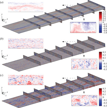
It is interesting to investigate whether our WMLES at  $Re_c=10^7$ can also capture the above described features. In figure 22, generally all three components
 $u$,
 $v$ and
 $w$ are ‘lighter’ compared with figures 20 and 21. This is expected because when using the same colour bar, a high-Reynolds-number flow indicates a smaller magnitude of velocity fluctuations. The two main features of figures 20 and 21, including the large-scale rolls on the wall-parallel plane of
 $u$ (figure 22a) and the smaller-scale features on the cross-flow plane images of
 $v$ and
 $w$ (figure 22b,c), are all found in this WMLES at
 $Re_c=10^7$.
Instantaneous velocity fields,  $Re_\tau \approx 2.8 \times 10^5$: (a) streamwise velocity
 $u$; (b) vertical velocity
 $v$; (c) spanwise velocity
 $w$.

8.2. Roll structure
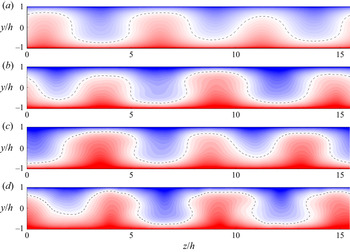
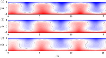
To demonstrate the present interpretation of rolls, we show colour contours of the averaged mean streamwise velocity field for five WRLES in figure 23 and four WMLES in figure 24. The streamwise velocity  $\tilde {u}$ is plotted to show its large fluctuations in each roll. A notable difference can be observed between
 $Re_\tau \approx 500$ and
 $Re_\tau \approx 2.8\times 10^5$. In figure 23(a), the zero line of
 $\tilde {u}$ shows a wavy behaviour which is similar to prior DNS (Lee & Moser Reference Lee and Moser2018). However, the zero line for
 $\tilde {u}$ for
 $Re_\tau \approx 2.8\times 10^5$ in figure 24(d) shows a more pronounced mushroom structure, which clearly enhances the mixing of the flows generated from two moving walls. It is plausible that this mushroom structure is unstable and that the rolls could potentially disappear in even higher
 $Re_c$ flows.
Contours of streamwise velocity  $\tilde {u}$. Wall-resolved LES: (a)
 $Re_\tau \approx 500$; (b)
 $Re_\tau \approx 1000$; (c)
 $Re_\tau \approx 1800$; (d)
 $Re_\tau \approx 3600$.

Contours of streamwise velocity  $\tilde {u}$. Wall-modelled LES: (a)
 $Re_\tau \approx 3600$; (b)
 $Re_\tau \approx 3.3 \times 10^4$; (c)
 $Re_\tau \approx 2.8 \times 10^5$.

8.3. Roll energy
Diagnostics suitable for characterizing roll behaviour are the kinetic-energy densities, which are defined in (3.4) as  $e_u(y)$,
 $e_v(y)$ and
 $e_w(y)$. Integration in the wall-normal direction provides an overall measure of the energy associated with the mean roll motion. We define
 $E_\phi$ as the integral of the corresponding
 $e_\phi (y)$ and
 $E_r$ as a combination of the
 $v$ and
 $w$ components. Specifically,
 \begin{equation} E_\phi = \frac{1}{2\,h} \int_{{-}h}^{h} e_\phi\, {\textrm{d} y} , \quad E_r = E_v + E_w, \end{equation}
where  $E_r$ can be interpreted as the kinetic energy of the mean motion in the large-scale rolls, while
 $E_u$ is the corresponding streamwise energy. Both are functions of
 $Re_\tau$.
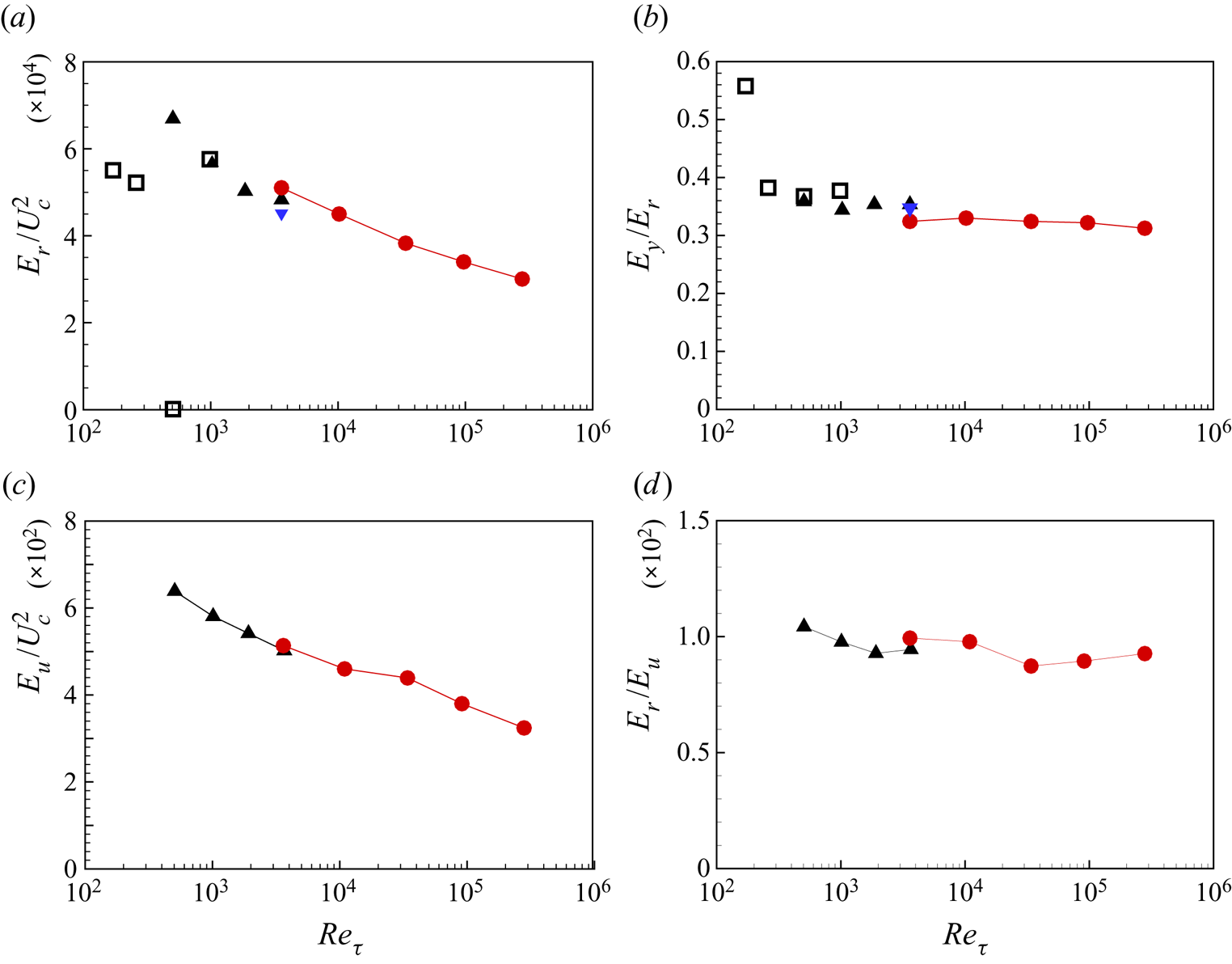
In figure 25(a), we plot  $E_r$ versus
 $Re_\tau$ from the present LES and DNS results from Pirozzoli et al. (Reference Pirozzoli, Bernardini and Orlandi2014). The two DNS data at low
 $Re_\tau$ are not discussed because these
 $Re_\tau$ are within the range of incipient roll generation. The LES data agrees fairly well with DNS at
 $Re_\tau \approx 500$ and
 $1000$. Wall-resolved LES at these two
 $Re_\tau$ do not clearly reveal a trend while the wall-modelled LES do show a sharp decline of
 $E_r$ with increasing
 $Re_\tau$, which implies a relative weakening of roll strength as
 $Re_\tau$ increases. The ratio
 $E_v/E_r$, which measures the wall-normal component contribution to the total roll energy, is shown in figure 25(b). With the exception of the DNS of
 $Re_\tau =171$ (Pirozzoli et al. Reference Pirozzoli, Bernardini and Orlandi2014), all other cases indicate a near-constant a value around 0.30–0.35. In figure 25(c), we plot
 $E_u/U_c^2$ for WRLES and WMLES while in figure 25(d), the corresponding plots for
 $E_r/E_u$ are shown. It is clear that for all LES,
 $E_r/E_u$ maintains a nearly constant level of approximately
 $1\,\%$, which is consistent with figure 5(b).
Roll energy diagnostics: (a) plot of  $E_r/U_c^2$ versus
 $Re_\tau$; (b) plot of
 $E_v/E_r$; (c) plot of
 $E_u/U_c^2$; (d) plot of
 $E_r/E_r$. Here,
 $\square$, reference DNS by Pirozzoli et al. (Reference Pirozzoli, Bernardini and Orlandi2014);
 $\blacktriangle$, wall-resolved LES;
 $\blacktriangledown$ (blue), coarse wall-modelled LES;
 $\bullet$ (red), wall-modelled LES.

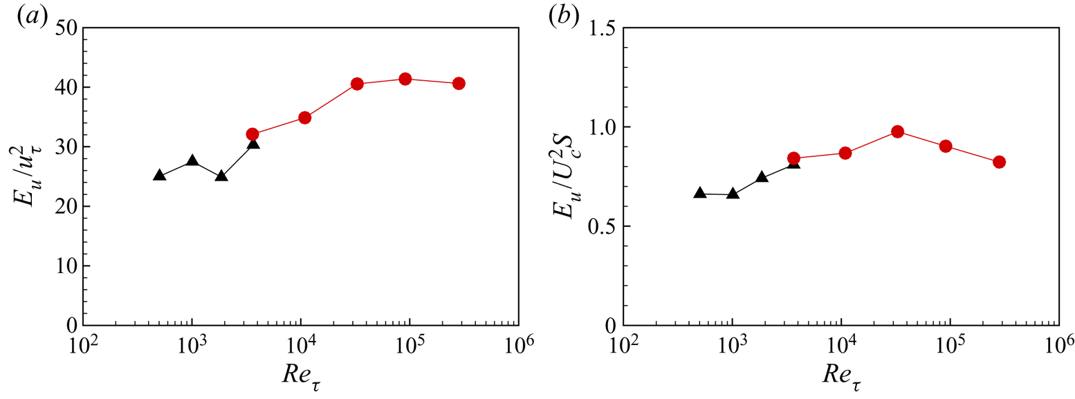
In addition to the above scaling of  $E_u$ using
 $U_c$, we further show scaling using
 $u_\tau$. In figure 26(a), we find that
 $E_u/u_\tau ^2$ does not decrease over two decades of
 $Re_\tau$. This may imply that while streamwise rolls may continue to weaken on outer scaling at quite high
 $Re_\tau$, they may survive on inner scaling. Figure 26(b) shows the plot of
 $E_u/(U_c^2 S)$. Its variation with
 $Re_\tau$ is generally around unity and does not show a clear tendency with increasing
 $Re_\tau$.
Roll energy scaling using  $u_\tau$ and
 $S$: (a) plot of
 $E_u/U_\tau ^2$ versus
 $Re_\tau$; (b) plot of
 $E_u/(U_c^2S)$. Here,
 $\square$, reference DNS by Pirozzoli et al. (Reference Pirozzoli, Bernardini and Orlandi2014);
 $\blacktriangle$, wall-resolved LES;
 $\bullet$ (red), wall-modelled LES.

8.4. Circulation
The roll circulation provides a further measure of the roll activity. This is implemented using the mean velocity field as shown in figures 23 and 24. A control area in the  $y\text {--}z$ plane is constructed comprising the top and bottom wall boundaries, a fixed left boundary
 $z/h = \textrm {const.}$ and a right boundary also with
 $z/h= \textrm {const}$. The circulation around this closed area can then be calculated as
 $\varGamma = \oint {\boldsymbol {u}}\boldsymbol {\cdot } \textrm {d}\boldsymbol {l}$. The normalized circulation
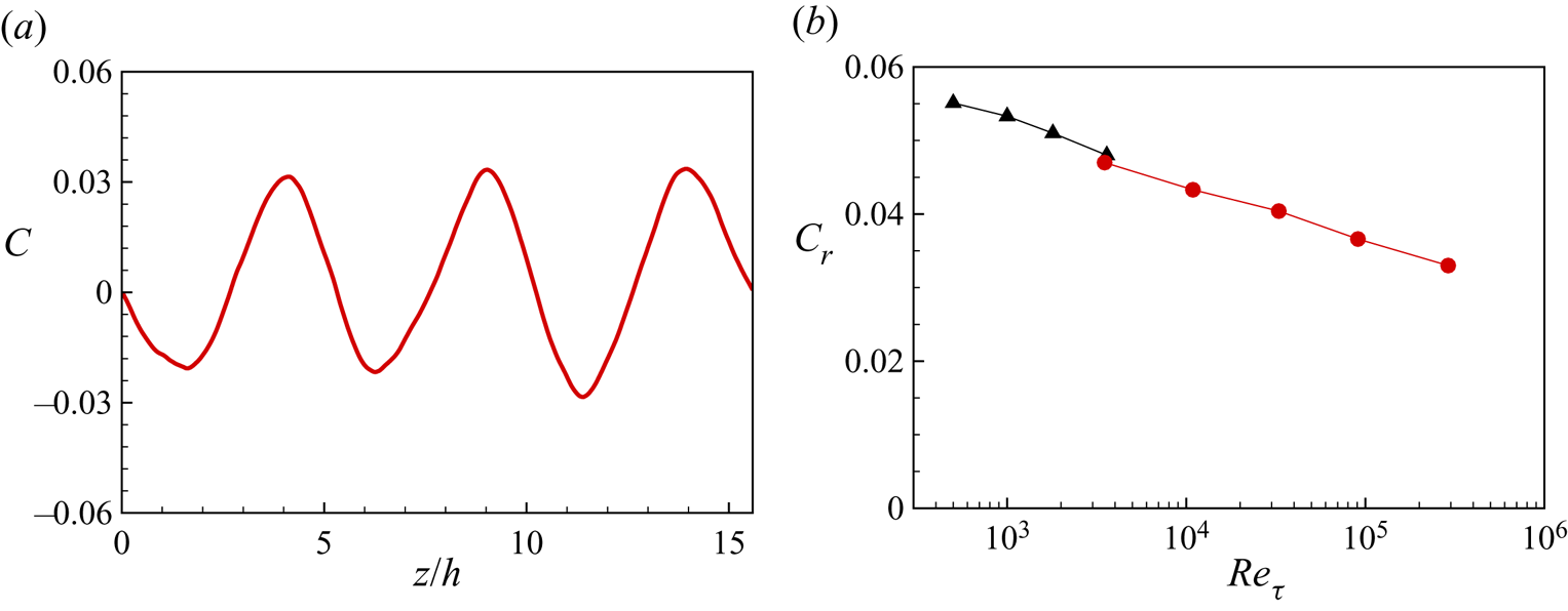
 $C = \varGamma /(U_c\,h)$ is plotted against the distance between the left and right boundaries in figure 27(a) for
 $Re_\tau \approx 500$. This shows oscillatory behaviour as the right-hand boundary passes through full rolls. We define the circulation per roll,
 $C_r$, as the average between maxima and minima of
 $C(z/h)$ across the spanwise flow domain. This is shown for both WRLES and WMLES as a function of
 $Re_\tau$ in figure 27(b). The trend with increasing
 $Re$ is similar to that for
 $E_r(Re_\tau )$. Both are consistent with diminishing relative roll strength as
 $Re_\tau$ increases. This is consistent with the hypothesis that the rolls may eventually dissipate and disappear at sufficiently large
 $Re_\tau$.
Circulation: (a) measure of circulation  $C$ for case at
 $Re_\tau \approx 500$; (b) roll circulation
 $C_r$ for all cases. Here,
 $\blacktriangle$, wall-resolved LES;
 $\bullet$ (red), wall-modelled LES.

9. Conclusion
It has been demonstrated that both wall-resolved and wall-modelled LES can be successfully applied to classical PC flow at fairly high plate Reynolds numbers. Both wall-resolved and wall-modelled LES capture the presence of streamwise rolls distributed across the spanwise domain. For friction Reynolds numbers  $Re_\tau$ in the in the range of
 $500 \sim 3600$, the wall-resolved LES results agree with available DNS results at lower Reynolds numbers, and show consistent trends at larger values. The wall-modelled LES are shown to give reasonable agreement with the wall-resolved LES for the streamwise mean velocity and the turbulence intensities at overlap Reynolds numbers. All mean-flow velocity profiles at different
 $Re_\tau$ show reasonable collapse and are consistent with a von Kármán constant of
 $0.4$. For the spanwise turbulent intensities, the outer part is suggestive of a log-like form, similar to the channel flow trend found via DNS at similar
 $Re_\tau$ by Lee & Moser (Reference Lee and Moser2018). The streamwise turbulence intensities show substantial differences in two distinct diagnostics. This is a result of the presence of the streamwise rolls.
The variation of  $Re_\tau$ as a function of the plate Reynolds number
 $Re_c$, agrees with a standard Lambert function relation across the whole range of
 $Re_\tau$ explored. The relation between
 $Re_c$ and the velocity gradient at the centreline,
 $S=f(Re_c)$, is well modelled by the matching of two log laws at the centreline, at least at our largest Reynolds number in the range
 $\sim 3.3\times 10^4 \text {--} 2.8\times 10^5$.
For the roll structure, we find that a relatively low-Reynolds-number flow shows a smooth and wavy zero-streamwise-velocity line across the span between two moving walls, while for our higher-Reynolds-number flow, a folding zero-velocity line emerges, which indicates differential flow about zero in the streamwise direction in the form of a mushroom-like structure. Measures of the mean-flow roll energy and the roll circulation indicate that this strong distortion tends to diminish the strength of rolls with increasing Reynolds number. Together with extrapolation of the model of § 7 to extremely large  $Re_\tau$, this suggests an infinite Reynolds-number-limit flow consisting of zero mean streamwise velocity across almost all of the wall-normal domain with vanishingly thin viscous domains at the plate walls, and with possibly asymptotically zero roll strength.
Funding
This work was partially supported by the KAUST baseline research funds of R.S. The Cray XC40, Shaheen, at KAUST was used for all the reported LES.
Declaration of interests
The authors report no conflict of interest.
Appendix A. Effect of spanwise extent at $Re_\tau = 500$

In the above LES, we employ a fixed spanwise domain  $L_z = 5{\rm \pi}$. This follows Lee & Moser (Reference Lee and Moser2018) who found three roll pairs and statistically stable results. A question of fundamental interest is the persistence and spanwise size of these structures for large spanwise domains.
Here we investigate the effect of spanwise domain size at  $Re_\tau =500$. With the previous streamwise domain
 $L_x$ unchanged, we compare four different values of
 $L_z= (5{\rm \pi},10{\rm \pi},20{\rm \pi},40{\rm \pi} )$. The corresponding mesh is increased to keep the same
 $L_z/N_z$ while the time-average period is generally approximately
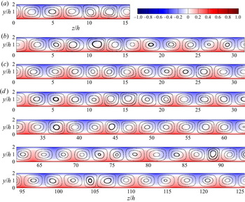
 $Tu_\tau /h = 50$. We first visualize the large-scale flow structures by plotting contours of both streamwise mean velocity and cross-flow streamlines formed by the mean vertical velocity and the mean spanwise velocity. These plots are shown in figure 28, where for all four cases, rolls are clearly observed.
Visualization of roll structures in cases with different span-wise domain,  $Re_\tau \approx 500$: (a)
 $L_z/h=5{\rm \pi}$; (b)
 $L_z/h=10{\rm \pi}$; (c)
 $L_z/h=20{\rm \pi}$; (d)
 $L_z/h=40{\rm \pi}$.

Various domain sizes have been used in the literature. Lee & Moser (Reference Lee and Moser2018) found three roll pairs in  $L_z = 5{\rm \pi}$, Avsarkisov et al. (Reference Avsarkisov, Hoyas, Oberlack and García-Galache2014) showed four pairs in
 $L_z = 6{\rm \pi}$ and Pirozzoli et al. (Reference Pirozzoli, Bernardini and Orlandi2014) showed five pairs with
 $L_z=8{\rm \pi}$. When estimating the roll size from one set of data, for example, a fixed span-wise domain size
 $L_z$ containing the number of rolls
 $N_p$, one could define a roll size
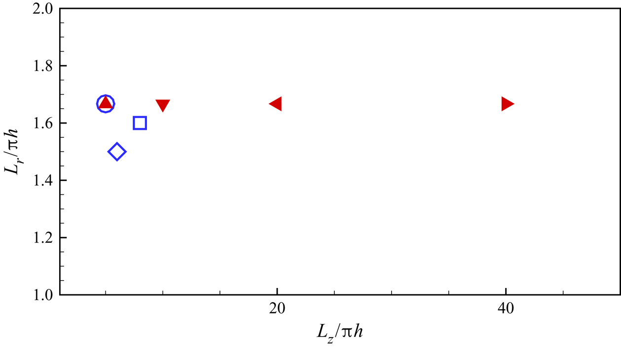
 $L_r = L_z / N_p$. In figure 29, we plot the present LES results for
 $L_r/({\rm \pi} \,h)$ versus
 $L_z/({\rm \pi} \,h)$ together with the three measurements from the above-discussed three DNS datasets. It shows the present LES, up to
 $L_z/h=40{\rm \pi}$, maintains a roll size of
 $L_r/h=5{\rm \pi} /3$.
Roll size  $L_r$,
 $Re_\tau \approx 500$. Hollow symbols are from reference DNS data. Filled symbols are present LES data. Here,
 $\circ$,
 $L_z/h=5{\rm \pi}$ by Lee & Moser (Reference Lee and Moser2018);
 $\diamond$,
 $L_z/h=6{\rm \pi}$ by Avsarkisov et al. (Reference Avsarkisov, Hoyas, Oberlack and García-Galache2014);
 $\square$,
 $L_z/h=8{\rm \pi}$ by Pirozzoli et al. (Reference Pirozzoli, Bernardini and Orlandi2014);
 $\blacktriangle$,
 $L_z/h=5{\rm \pi}$;
 $\blacktriangledown$,
 $L_z/h=10{\rm \pi}$;
 $\blacktriangleleft$,
 $L_z/h=20{\rm \pi}$;
 $\blacktriangleright$,
 $L_z/h=40{\rm \pi}$.

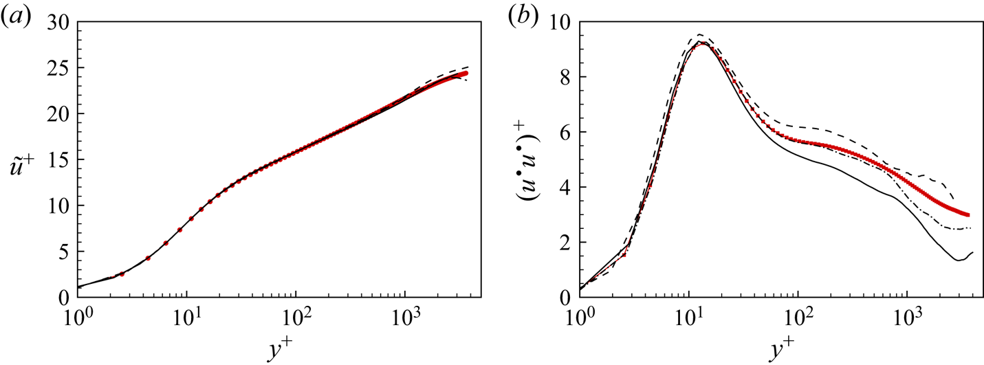
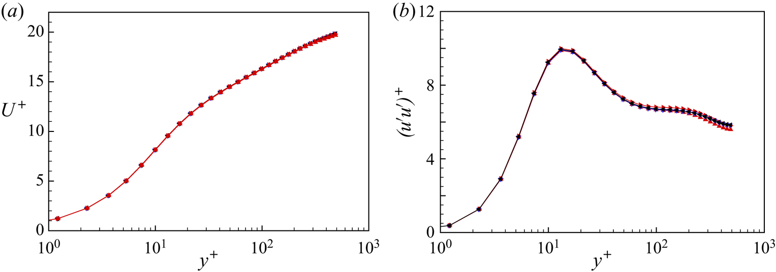
It is also of interest to investigate the effect of the spanwise domain on one-point diagnostics. In figure 30, we compare the mean streamwise velocity profile and the streamwise turbulence intensity for the four cases. There is generally a quite small domain effect, which confirms that one-point diagnostics are not sensitive to the spanwise domain. This is consistent with previous DNS studies, including the comparison of the streamwise domain effect by Lee & Moser (Reference Lee and Moser2018).
Comparison of mean streamwise velocity (a) and turbulence intensity (b) for cases with different spanwise domains,  $Re_\tau \approx 500$. Here,
 $\blacktriangle$,
 $L_z/h=5{\rm \pi}$;
 $\blacktriangledown$,
 $L_z/h=10{\rm \pi}$;
 $\blacktriangleleft$,
 $L_z/h=20{\rm \pi}$;
 $\blacktriangleright$,
 $L_z/h=40{\rm \pi}$.

Appendix B. Comparison between cases with and without SGS model
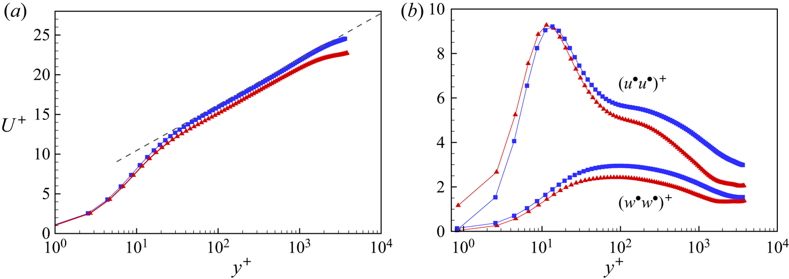
The LES closure employs different models. For WRLES, only an SGS model is required, while for WMLES, an additional virtual-wall model is necessary. Here we investigate no-model LES. Mean velocity profiles are compared in figure 31(a) for both WRLES and no-SGS-model LES at  $Re_\tau \approx 3600$. The no-SGS case shows a systematically lower profile and also a much smoothened flow near the mid-span plane. The same trend is observed at lower
 $Re_\tau \approx 1000$ (not shown), where the WRLES agrees well with Pirozzoli et al. (Reference Pirozzoli, Bernardini and Orlandi2014) but the no-SGS-model simulation does not. We also compare the streamwise and spanwise turbulence intensities in figure 31(b). Both the intensities show significant differences between the WRLES and no-SGS-model cases. Generally, the intensities are underestimated in the core region.
Comparison between the WRLES (symbol  $\blacksquare$) and no-SGS (symbol
 $\blacktriangle$) cases,
 $Re_\tau \approx 3600$. (a) Streamwise velocity
 $U^+$. Dashed line, log law of
 $U^+ = \ln y^+/0.4 + 5.0$. (b) Turbulence intensity
 $(u^\bullet u^\bullet )^+$ and
 $(w^\bullet w^\bullet )^+$.

In WMLES,  $u_\tau$ is computed dynamically with the time evolution of the flow and is used to provide a Dirichlet boundary condition for the next-step velocity update. For the no-SGS-model plus no-wall-model LES at our larger values of
 $Re_\tau$ and at the same mesh resolution, the code always crashed, with no results. The wall model is thus necessary at large
 $Re_\tau$ where the near-wall flow cannot be resolved.