This article presents forecasts of the 2012 presidential and US House of Representatives elections. The presidential forecasts are of the national two-party presidential vote percentage for the in-party candidate and are based on the trial-heat and economy forecasting equation and its companion convention-bump equation. The House election forecast is of the net seat change for the Democratic Party from 2010 to 2012. This forecast is produced from two versions of a seats-in-trouble forecasting equation.
Although the presidential and congressional forecasting equations have no predictor variables in common, the reasoning behind them is the same. Three elements are common to all the equations. First, each starts with a reading of where the election stands at the outset of the campaign when the forecast is made. Second, contextual variables are added that tap into the circumstances and political climate in which the campaign takes place and that have not already been fully incorporated into the electorate's precampaign preferences. Finally, the relationships of both sets of variables to election outcomes are estimated using historical data to determine how initial inclinations and the campaign's context typically shape election outcomes. A theory of predictable campaign effects underlies these models (Campbell Reference Campbell2008).
THE PRESIDENTIAL VOTE FORECASTING MODELS
The presidential vote forecast is from the Trial-Heat and Economy Forecasting Model developed in 1990 (Campbell and Wink Reference Campbell and Wink1990). It built on Lewis-Beck and Rice's earlier work (Lewis-Beck Reference Lewis-Beck1985, 58) and an analysis of the accuracy of Gallup preference polls at various points in campaigns. The equation involves only two predictors: the percentage of registered voters indicating a preference for the in-party presidential candidate in the Gallup Poll around Labor Day and the second-quarter growth rate in real gross domestic product (GDP), adjusted for a neutral point of 2.5 percentage points and discounted for nonincumbent or successor candidates of the in-party. Analyses of the equation using preference polls at various points in the campaign season found no appreciable gains in prediction accuracy after early September (Campbell and Wink Reference Campbell and Wink1990). An analysis of various time frames of economic conditions also found that the second-quarter growth rate was the strongest indicator of the economic climate available for forecasting that had not already been considered by voters at Labor Day, but would affect how voter evaluations evolved during the campaign (Campbell Reference Campbell2008). The adjustment to the economic growth variable takes into account the conditional nature of retrospective voting in which nonincumbents are accorded partial credit or blame for the record of the incumbent (Campbell Reference Campbell2001; Campbell, Dettrey, and Yin Reference Campbell, Dettrey and Yin2010; Holbrook Reference Holbrook2008; Nadeau and Lewis-Beck Reference Nadeau and Lewis-Beck2001; Norpoth Reference Norpoth, Dorussen and Taylor2002).
This model, with some minor changes, has predicted the popular vote in five presidential elections. With one notable exception (the 2008 election, more on that shortly), it has been quite accurate. Setting aside 2008, the average absolute error of actual predictions has been 2.4 percentage points and the median out-of-sample error is only 1.2 percentage points.
In 2004, I developed the convention-bump and economy equation as a companion to the Trial-Heat and Economy Model. This equation includes three predictor variables: the in-party candidate's share of support in Gallup's preference poll before the parties' first convention, the poll change or “convention bump” from before the first convention to after the second convention, and the second quarter's real GDP growth rate variable used in the trial-heat equation (with the same centering and open-seat adjustments). The inclusion of the convention-bump variable recognizes that a larger than usual portion of poll leads produced during the convention period dissipate after the conventions (Campbell Reference Campbell2008; Campbell, Cherry, and Wink Reference Campbell, Cherry and Wink1992). The median out-of-sample error of this equation (setting aside 2008) is 1.6 percentage points.
Before applying these equations to forecast the 2012 election, two recent complications for this year's forecasts should be addressed. The first concerns the timing of the national conventions. The second concerns the extraordinary events that intervened during the 2008 campaign and whether 2008 should be used in estimating forecasting equations.
The Convention Timing Complication
A premise of the Trial-Heat and Economy Model is that preference polls at Labor Day of the election year, the traditional kick-off date of the fall campaign, are a stable indicator of where public opinion stands at the outset of the campaign. This appeared to be a fairly safe assumption, until recently. Before the 2004 election, the second national nominating conventions of the major parties had been held no later than mid- to late-August. This scheduling allowed short-term convention-bump effects in the polls to subside before Labor Day. In 2004 and in 2008, however, because of campaign financing considerations, the conventions were scheduled later. The Republican conventions in those years spilled over into the first few days of September. This year, the Democratic convention does not even begin until Labor Day.
Because of the new conflict between the Trial-Heat Model's forecasting schedule and the party's convention schedules, the trial-heat poll used by the model will be pushed back to September 10. This is later than normal, but only a few days closer to the election than the usual 60-day lead time. Even so, because the “Labor Day” poll is only a couple of days removed from the Democratic convention, it is likely to reflect some short-term effects of the convention bump. In light of this, it may be advisable to pay particular attention to the forecast of the Convention-Bump Model this year.
The Wall Street Meltdown Complication of 2008
The second complication involves the 2008 election. Election forecasting is premised on the idea that normal elections are predictable because we know how precampaign fundamentals affected normal elections in the past. Election forecasting models are essentially systematic ways of learning from history and applying that knowledge to future elections. Lessons from past normal elections allow the prediction of future normal elections.
The normal election premise entails an assumption that nothing cataclysmic occurs during the campaign to derail the “playing out” of the fundamentals in the campaign. The idea is that lessons learned from the general history of normal elections are not helpful to predicting elections in which a catastrophic event intervened between the forecast and the election. By the same token, we cannot learn how fundamentals affect the vote from an election in which the fundamentals were overridden by a crisis. An aberrant election may be more misleading than enlightening about how the fundamentals work.
Fortunately for forecasting, aberrant elections are infrequent. History is replete, however, with events that could have derailed forecasts had they occurred during a campaign. “October Surprises” are quite possible. For instance, suppose that the terrorist attacks of September 11 had occurred in 2000 or in 2004 instead of in 2001. Is there any doubt that the fundamentals in those elections would have been trumped by the unforeseen crisis?
In the 2008 campaign, an unforeseen crisis of a different sort, the Wall Street Meltdown, intervened between the forecasts and the vote (Campbell Reference Campbell2010a). It derailed the likely effects of the fundamentals and rendered the forecasts moot. Three pieces of evidence lead to the conclusion that the 2008 election violated the normal election assumption: (1) the financial meltdown was unanticipated, (2) it sent the economy into a tailspin during the campaign, and (3) the economic collapse had major political repercussions for the election. The 2008 election was not a normal election in which the fundamentals “played out.”
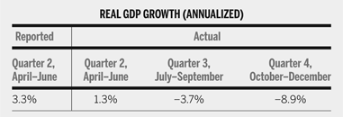
Neither economic nor election forecasters anticipated the Wall Street Meltdown, much less that it would take place during the campaign. In late August, the Bureau of Economic Analysis (BEA) estimated second-quarter GDP growth at 3.3%. This was good economic news and a number that several election forecasters used in their models. Based on the normal correlation of economic growth rates from one quarter to the next (r = .38), one would have expected third-quarter growth of about 2.8%. Well into the third-quarter, economic forecasters predicted slower third-quarter growth (1.2%) (Survey of Professional Forecasters 2008). According to analyses using the Leading Economic Index (LEI), growth of about .8% to 1.9% in GDP was expected (Campbell Reference Campbell2011). The LEI actually increased in September (Conference Board 2008). In short, to one degree or another, all signs in 2008 pointed to a preelection economy that was, at worst, sluggish. There were no signs of a collapse in the immediate offing.
Second, as table 1 documents, the meltdown of financial institutions sent the economy into a tailspin. The economy contracted by nearly four percentage points in the third quarter, much of that apparently in September. And while only about five weeks of the fourth quarter preceded the election, the economy continued spiraling downward during these weeks, contracting at a rate of nearly nine percentage points.
The Wall Street Meltdown's Economic Meltdown, 2008

Note: The reported second quarter growth rate of real GDP was from the August 2008 release of the Bureau of Economic Analysis. The estimates of actual real GDP growth are from the Bureau of Economic Analysis as of June 28, 2012.
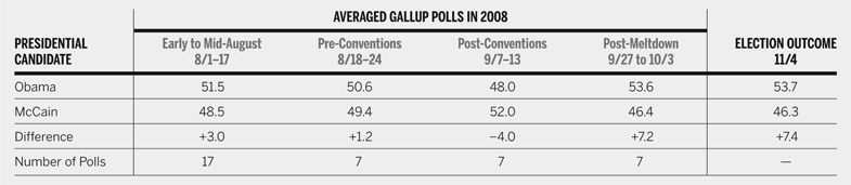
The financial crisis and the unexpected economic nosedive were politically devastating for the in-party. Table 2 reports the preference polls from August to Election Day. Each point examined in the campaign is based on at least a week's worth of Gallup's polling. As the table shows, Obama held a small lead over McCain through the first few weeks of August, but the race had narrowed to a virtual tie in the week before the first convention. McCain emerged from the conventions with a four-point lead. Even with the normal erosion of much of the convention bump, the election appeared on track for a very close finish with a slight edge to McCain. This was consistent with the trial-heat forecast (52.7% for McCain).Footnote 1 Then the financial system collapsed. The public understood immediately the gravity of the situation. Forty percent of respondents to a USA Today and Gallup Poll in late September called the situation “the biggest financial crisis in [their] lifetime” (Polling Report 2008). From mid-September to the first few days of October, McCain dropped from being four points ahead to seven points behind. President Bush's already low approval ratings took a similar hit. The post-meltdown standing of the candidates is about where the election wound up.
The Wall Street Meltdown's Political Meltdown, 2008

Because of the economic collapse in the midst of the campaign, 2008 should be regarded as an aberrant election. As such, I have excluded it from the estimation of the presidential equations. For skeptics of this decision, I also estimated the model with 2008 included (not shown). Although the 2008-included estimates reduce explained variance and increase out-of-sample errors, they leave the predictor coefficients within .02 of the 2008-excluded estimates.
The Presidential Forecast for 2012
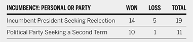
President Obama enters the 2012 election with a significant advantage. As table 3 shows, the electorate is inclined to retain incumbent presidents, especially if the president's party has been in the White House for one term. There is a presidential incumbency advantage (Campbell Reference Campbell, Campbell and Garand2000, Reference Campbell2008; Fair Reference Fair1978; Mayhew Reference Mayhew2008; Weisberg Reference Weisberg2002). The range of the vote for incumbent races has been from landslides in their favor (Johnson, Nixon, and Reagan) to narrow or moderate size losses (Carter and G.H.W. Bush).
Incumbency and Presidential Election Outcomes, 1900–2008

Note: Reelection includes incumbent presidents who had not been previously elected to the office (T. Roosevelt, Coolidge, Truman, Johnson, and Ford).
Beyond incumbency, however, the political climate of 2012 suggests a close election. The parties are near parity and the electorate is polarized. President Obama's approval ratings through the summer hovered in the mid- to high-40s, survivable but not thrive-able. The economy has been weak throughout Obama's term. Unemployment rates have been 8% or higher for 42 consecutive months as of July 2012. Since June 2009, when the recession associated with the Wall Street Meltdown ended (National Bureau of Economic Research 2012), there have been only two quarters (out of 12) in which real economic growth exceeded 2.6%. From the second year of his term through the first half of the election year (10 quarters), the mean quarterly economic growth during the Obama presidency has been only 2.1 percentage points. In terms of economic growth, he ranks eighth out of the last 10 presidents who sought reelection. The two presidents with weaker economies (George H.W. Bush and Gerald Ford) both lost. Six of the seven presidents presiding over stronger economies won. Carter, with a mean growth rate of 2.6 percentage points, was the exception. Growth in 2012's first quarter was an anemic 2%, and the initial estimate of second quarter growth was only 1.5%. Jimmy Carter is the only president seeking reelection in the post-WWII era who entered the fall campaign with a weaker second quarter economic number. It is difficult to see his economic record as anything but a serious liability for President Obama.
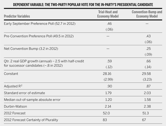
The Trial-Heat and Convention-Bump Models provide more specific readings of the historical effects of incumbency (implicit in the in-party orientation of the equations), the early inclinations of the electorate, and the latest reading of economic conditions as the fall campaign begins. Table 4 presents the trial-heat and economy equation as well as the convention-bump and economy forecasting equation. Each of the models starts with a reading of where the electorate stands at the outset of the campaign and adds adjustments for how the campaign is likely to alter those stands based on the competitiveness of the campaign (the discount of the initial poll standing), incumbency (the intercept when other factors are neutral), the second-quarter growth in the economy (itself adjusted to a neutral level and discounted for open-seat races), and, in the case of the Convention-Bump Model, the temporary portion of convention effects on the race. In essence, this is a more sophisticated reading of the polls, taking both their historical and contemporary contexts into account.
Trial-Heat and Convention-Bump Forecasting Models, 1948–2004

Note: N = 15. Standard errors are in parentheses. These estimates differ slightly from the 2008 values because they use Gaines's calculation of the 1960 vote (Gaines 2001). The 2008 case was not included in the estimation because the unprecedented and unanticipated financial meltdown intervened between the forecast and the election. With 2008 included, the adjusted R2 drops to .81 in the trial-heat model and .80 in the convention-bump model. The coefficients change by .02 or less with the inclusion of 2008.
The trial-heat and economy equation indicates that Barack Obama is likely to receive 52.0% of the two-party vote. Based on the distribution of out-of-sample errors, the likelihood that Obama will receive a plurality of the national popular vote is 83%. The forecast is based on President Obama having 52.7% of the two-party support in Gallup's preference poll released on September 10 (Gallup 2012) and an annualized real GDP growth rate of 1.7% in the second quarter (April–June) of 2012 as indicated by the BEA's second estimate released at the end of August (Bureau of Economic Analysis 2012). The growth rate is converted to an economic index by subtracting 2.5 percentage points from it. It is not halved in 2012, because the in-party candidate is the incumbent.
The convention bump and economy equation indicates that Barack Obama is likely to receive 51.3% of the two-party vote. Based on out-of-sample errors, the likelihood of an Obama plurality is 67%. This forecast is based on President Obama having 49.5% of the support of registered voters in Gallup's last preference poll before the conventions, a net convention bump for President Obama of 3.2%, and the economic variable used in the trial-heat equation.
THE SEATS-IN-TROUBLE HOUSE FORECASTING MODEL
The receptiveness of the next Congress to whoever is elected president depends substantially on the partisan composition of the US House and the Senate. The seats-in-trouble forecasting equation is designed to predict the likely party makeup of the US House. The equation, developed for the 2010 midterm election, predicts the net partisan change in US House seats for Democrats (Campbell Reference Campbell2010b).
Like the presidential models, the core of this model is a reading of where things stand with voters before the campaign is fully underway. This core variable is the seats-in-trouble variable, the difference in the number of seats held by each party that are in substantial jeopardy of being lost. The seats-in-trouble variable is constructed from the district-by-district handicapping of House races by The Cook Political Report.Footnote 2 These ratings assign each House race to one of eight categories—solid, likely, leaning, or toss-up for either party. The number of seats deemed to be “in trouble” are those won in the previous election by a party but are now not in that party's solid, likely, or leaning categories. This coding was developed after examining the win-rates for seats in each of the categories. The variable is computed as the net party difference of seats-in-trouble, the number of Democratic seats-in-trouble minus the number of Republican seats-in-trouble. This index has ranged from a 44-seat Republican advantage in 2010 to a 27-seat Democratic advantage in 2008. Cook's latest ratings between July and the first day of September are used in the calculations. The 1986 and 1990 elections could not be used because The Cook Political Report did not handicap races within this time frame.
In 2010, the first year in which the model was tested in real time, it predicted the Republicans landslide. Republicans were predicted to gain 51 or 52 seats. They actually gained 64 seats. Although off by about a dozen seats, no other forecast in late August was more accurate, and Republican seat gains in 2010 were larger than anything that had been experienced in the previous half century, including the Republican break-through election of 1994.
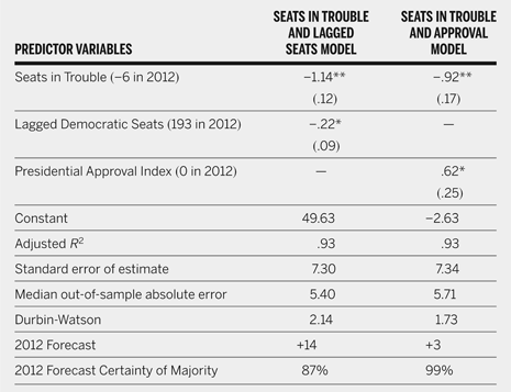
Although the seats-in-trouble variable is the key predictor, two different contextual variables are included in the twin equations. The first is the Democratic Party's seat holdings going into the election. This variable is included to reflect the fact that you cannot gain seats you already have and that gaining seats is more difficult starting from a higher base. The second contextual variable is the president's approval rating. This is normed to 45 in on-year elections and oriented to reflect the president's party. Table 5 presents the updated estimates of two versions of the seats-in-trouble forecasting model. The equation is estimated over 12 elections, both on-year and midterms, from 1984 to 2010.Footnote 3
The Seats in Trouble Forecasting Equations of Seat Change for the Democrats in the US House, 1984–2010

Note: N = 12. Standard errors are in parentheses. The 1986 and 1990 elections are not included because of the unavailability of the “seats in trouble” measure in those years.
What do the seats-in-trouble equations forecast for 2012? Based on data from The Cook Political Report as of August 20, Reference Cook2012, the net seats-in-trouble index is −6, with the Democrats having 15 seats in trouble and the Republicans having 21. With Democrats having won 193 seats in 2010 and with President Obama's approval index standing at zero (late August approval rating of 45 minus 45), the Seats-in-Trouble Model forecasts that Democrats will gain about 3 to 14 seats. Based on the equations' out-of-sample errors, the probability that Republicans will maintain their control of the House of Representatives is between 87% and 99%.