1 Introduction
In the last few decades, electron–positron (e–p) plasmas have attracted significant interest amongst researchers. The study of nonlinear effects in e–p plasmas is important since it is known that these plasmas exists in pulsars (Goldreich & Julian Reference Goldreich and Julian1969; Michel Reference Michel1982), active galactic nuclei (Miller & Witta Reference Miller and Witta1987), gamma-ray bursts (GRBs) (Piran Reference Piran2005), white dwarfs (Kashiyama, Ioka & Kawanaka Reference Kashiyama, Ioka and Kawanaka2011) and have also been studied in laboratory experiments (Greaves & Surko Reference Greaves and Surko1995). In these plasmas, there exists only one frequency scale, due to the same charge-to-mass ratio for the oppositely charged species. Hence they are different from their electron–ion counterparts and thus exhibit different wave phenomena.
It is thought that most of the e–p plasmas produced in astrophysical settings are of relativistic nature. The process by which a pulsar magnetosphere is populated with relativistic e–p plasma is assumed to be the decay of photons emitted by primary particles into secondary pairs. Synchrotron emission from these secondary pairs is then assumed to contribute to the high-energy emission from some pulsars. The choice of a relativistic or non-relativistic character for the distribution function of the involved particles is intimately related to the process of formation of the pairs (Asseo & Riazuelo Reference Asseo and Riazuelo2000; Weise & Melrose Reference Weise and Melrose2002). It is, therefore, plausible that non-relativistic astrophysical e–p plasmas may exist, given the effect of efficient cooling by cyclotron emissions (Zank & Greaves Reference Zank and Greaves1995; Bhattacharyya, Janaki & Dasgupta Reference Bhattacharyya, Janaki and Dasgupta2003). There is a vast body of literature dealing with linear and nonlinear wave propagation in e–p plasmas which are non-relativistic (Iwamoto Reference Iwamoto1993; Zank & Greaves Reference Zank and Greaves1995; Verheest et al. Reference Verheest, Hellberg, Gray and Mace1996; Esfandyari-Kalejahi, Kourakis & Shukla Reference Esfandyari-Kalejahi, Kourakis and Shukla2006). A simple two-fluid model was used to study the linear and nonlinear wave phenomena in electrostatic and electromagnetic solitary waves by Zank & Greaves (Reference Zank and Greaves1995). This linear study showed that many wave phenomena found in conventional electron–ion plasmas exist in a modified form in e–p plasmas. In their nonlinear analysis they found that only subsonic solutions exist, while the pulse width, rather than its amplitude, is related to the wave speed. Their results also showed that increasing the Mach number narrows the pulse width significantly, without any change in the amplitude.
Lu et al. (Reference Lu, Liu, Wang, Stenflo, Popel and Yu2010) investigated nonlinear electrostatic waves in an e–p plasma in the presence of background ions. They found that both smooth and spiky quasistationary waves were found to exist. They reported that as the wave speed increases, the nonlinearity of the wave decreases. They also pointed out that their results may be useful in understanding astrophysical and laboratory wave phenomena involving pair production and positron emissions. Liu & Liu (Reference Liu and Liu2011) investigated the formation of large-amplitude electromagnetic solitons with spiky structures in e–p plasmas. They pointed out that the localized electric field structures are important in understanding astrophysical objects, which could account for pulsar radio emissions. Spiky Langmuir solitons in a dense ultrarelativistic e–p plasma have been studied by Mofiz & Mamun (Reference Mofiz and Mamun1992) and Mofiz & Amin (Reference Mofiz and Amin2013). Mofiz & Amin (Reference Mofiz and Amin2013) used the two-fluid magnetohydrodynamic (MHD) equations to describe the e–p plasma, and found spiky Langmuir solitons that propagated along the open field lines of a pulsar magnetosphere, indicating that there is some association with pulsar radio emissions. Stark et al. (Reference Stark, Diver, da Costa and Laing2007) investigated a possible emission mechanism through the coupling of electrostatic oscillations with propagating electromagnetic waves using an e–p plasma model relevant to pulsar magnetospheres.
On the other hand, satellite observations in the Earth’s magnetosphere have also shown the existence of electrostatic solitary waves as part of broadband electrostatic noise (BEN). The (GEOTAIL (Matsumoto et al. Reference Matsumoto, Kojima, Miyatake, Omura, Okada, Nagano and Tsutsui1994, Reference Matsumoto, Kojima, Kasaba, Miyake, Anderson and Mukai1997; Kojima et al. Reference Kojima, Ohtsuka, Matsumoto, Omura, Anderson, Saito, Mukai, Kokubun and Yamamoto1999), POLAR (Franz, Kintner & Pickett Reference Franz, Kintner and Pickett1998) and FAST (Ergun et al. Reference Ergun, Carlson, McFadden, Mozer, Delroy, Peria, Chaston, Temerin, Elphic and Strangeway1998)) satellites frequently observed BEN and ESWs in various regions of the Earth’s magnetosphere. The characteristic feature of ESWs is solitary bipolar pulses and consist of small scale, large amplitude, parallel electric fields. These large-amplitude spiky structures have been interpreted in terms of either solitons (Temerin et al. Reference Temerin, Cerny, Lotko and Mozer1982) or isolated electron holes in the phase space corresponding to positive electrostatic potential (Omura et al. Reference Omura, Kojima and Matsumoto1994). Given that e–p plasmas are increasingly observed in astrophysical environments, as well as in laboratory experiments, the above mentioned satellite observations also lead us to explore if such nonlinear structures are also possible in e–p plasmas.
There is a distinct possibility that a pulsar magnetosphere can support the coexistence of two types of cold and hot e–p populations (Sturrock Reference Sturrock1971; Bharuthram Reference Bharuthram1992; Lazarus et al. Reference Lazarus, Bharuthram, Singh, Pillay and Lakhina2012). Linear electrostatic waves (Lazarus et al. Reference Lazarus, Bharuthram, Singh, Pillay and Lakhina2012) and solitary waves (Lazarus, Bharuthram & Hellberg Reference Lazarus, Bharuthram and Hellberg2008) have been studied in such a system. Here, we will investigate the possibility of nonlinear electrostatic spiky structures in a magnetized four component two-temperature e–p plasma. The paper is structured as follows. In § 2, the basic equations for the e–p plasma are presented. In § 3 we present the numerical results. A summary of our findings is presented in § 4.
2 Basic theory
The model considered here is a homogeneous magnetized, four component, collisionless, e–p plasma, consisting of cool electrons (ec) and cool positrons (pc) with equal temperatures
 $T_{c}$
and initial densities (
 $n_{ec0}=n_{pc0}$
), and hot electrons (eh) and hot positrons (ph) with equal temperatures
 $T_{h}$
and densities (
 $n_{eh0}=n_{ph0}$
). Wave propagation is taken in the
 $x$
-direction at an angle
 ${\it\theta}$
to the magnetic field
 $\boldsymbol{B}_{0}$
, which is assumed to be in the
 $x$
–
 $z$
plane.
The continuity and momentum equations for the four species are given by
 $$\begin{eqnarray}\displaystyle & \displaystyle \frac{\partial n_{j}}{\partial t}+\frac{\partial (n_{j}v_{jx})}{\partial x}=0 & \displaystyle\end{eqnarray}$$
 $$\begin{eqnarray}\displaystyle & \displaystyle \frac{\partial v_{jx}}{\partial t}+v_{jx}\frac{\partial v_{jx}}{\partial x}+\frac{1}{n_{j}m}\frac{\partial p_{j}}{\partial x}=-\frac{{\it\epsilon}_{j}e}{m}\frac{\partial {\it\phi}}{\partial x}+{\it\epsilon}_{j}{\it\Omega}v_{jy}\sin {\it\theta} & \displaystyle\end{eqnarray}$$
 $$\begin{eqnarray}\displaystyle & \displaystyle \frac{\partial v_{jy}}{\partial t}+v_{jx}\frac{\partial v_{jy}}{\partial x}={\it\epsilon}_{j}{\it\Omega}v_{jz}\cos {\it\theta}-{\it\epsilon}_{j}{\it\Omega}v_{jx}\sin {\it\theta} & \displaystyle\end{eqnarray}$$
 $$\begin{eqnarray}\displaystyle & \displaystyle \frac{\partial v_{jz}}{\partial t}+v_{jx}\frac{\partial v_{jz}}{\partial x}=-{\it\epsilon}_{j}{\it\Omega}v_{jy}\cos {\it\theta}, & \displaystyle\end{eqnarray}$$
 ${\it\epsilon}_{j}=+1(-1)$
for positrons (electrons) and
 $j=ec,pc,eh,ph$
for the cool electrons, cool positrons, hot electrons and the hot positrons, respectively.
The density of the cool electrons (positrons) is
 $n_{ec}$
(
 $n_{pc}$
), and that of the hot electrons (positrons) is
 $n_{eh}$
(
 $n_{ph}$
).
The general equation of state for the four species is given by
 $$\begin{eqnarray}\frac{\partial p_{j}}{\partial t}+v_{jx}\frac{\partial p_{j}}{\partial x}+3p_{j}\frac{\partial v_{jx}}{\partial x}=0.\end{eqnarray}$$
The system is closed by the Poisson equation
 $$\begin{eqnarray}{\it\varepsilon}_{0}\frac{\partial ^{2}{\it\phi}}{\partial x^{2}}=-e(n_{pc}-n_{ec}+n_{ph}-n_{eh}).\end{eqnarray}$$
In the above equations,
 $n_{j}$
,
 $\boldsymbol{v}_{j}$
and
 $p_{j}$
are the densities, fluid velocities and pressures, respectively, of the
 $j$
th species.
 ${\it\Omega}={\it\Omega}_{e}={\it\Omega}_{p}=eB_{0}/m$
is the cyclotron frequency. Here
 $m=m_{e}=m_{p}$
is the common mass of the electrons and the positrons. Adiabatic compression,
 ${\it\gamma}=(2+N)/N=3$
, is assumed, where
 $N=1$
implies one degree of freedom.
2.1 Linear analysis
Linearizing and combining equations (2.1)–(2.6) yields the following general dispersion relation for a four component e–p plasma:
 $$\begin{eqnarray}\displaystyle {\it\omega}^{2}=\frac{2{\it\omega}_{pc}^{2}({\it\omega}^{2}-{\it\Omega}^{2}\cos ^{2}{\it\theta})}{{\it\omega}^{2}-{\it\Omega}^{2}-\displaystyle \frac{3k^{2}v_{tc}^{2}}{{\it\omega}^{2}}({\it\omega}^{2}-{\it\Omega}^{2}\cos ^{2}{\it\theta})}+\frac{2{\it\omega}_{ph}^{2}({\it\omega}^{2}-{\it\Omega}^{2}\cos ^{2}{\it\theta})}{{\it\omega}^{2}-{\it\Omega}^{2}-\displaystyle \frac{3k^{2}v_{th}^{2}}{{\it\omega}^{2}}({\it\omega}^{2}-{\it\Omega}^{2}\cos ^{2}{\it\theta})}, & & \displaystyle\end{eqnarray}$$
where
 ${\it\omega}_{pc,ph}=(n_{0c,h}e^{2}/{\it\varepsilon}_{0}m)^{1/2}$
are the plasma frequencies of the cool and hot species, respectively.
In the limit
 $v_{tc}\ll {\it\omega}/k\ll v_{th}$
, where
 $v_{th}=(T_{h}/m)^{1/2}$
and
 $v_{tc}=(T_{c}/m)^{1/2}$
are the thermal velocities of the hot (cool) species, the dispersion relation (2.7) becomes,
 $$\begin{eqnarray}{\it\omega}^{4}-{\it\omega}^{2}({\it\Omega}^{2}+2{\it\omega}_{s}^{2}+3k^{2}v_{tc}^{2})+2{\it\omega}_{s}^{2}{\it\Omega}^{2}\cos ^{2}{\it\theta}=0,\end{eqnarray}$$
where
 ${\it\omega}_{s}={\it\omega}_{pc}/(1+2/3k^{2}{\it\lambda}_{Dh}^{2})^{1/2}$
and
 ${\it\lambda}_{Dh}=({\it\varepsilon}_{0}T_{h}/n_{oh}e^{2})^{1/2}$
.
Equation (2.8) yields
 $$\begin{eqnarray}\displaystyle {\it\omega}^{2}=\frac{1}{2}({\it\Omega}^{2}+2{\it\omega}_{s}^{2}+3k^{2}v_{tc}^{2})\left[1\pm \sqrt{1-\frac{(8{\it\omega}_{s}^{2}{\it\Omega}^{2}\cos ^{2}{\it\theta})}{({\it\Omega}^{2}+2{\it\omega}_{s}^{2}+3k^{2}v_{tc}^{2})^{2}}}\right]. & & \displaystyle\end{eqnarray}$$
In the limit
 $(8{\it\omega}_{s}^{2}{\it\Omega}^{2}\cos ^{2}{\it\theta})\ll ({\it\Omega}^{2}+2{\it\omega}_{s}^{2}+3k^{2}v_{tc}^{2})^{2}$
, (2.9) yields two modes. The positive sign gives the cyclotron mode,
 $$\begin{eqnarray}{\it\omega}_{+}^{2}=({\it\Omega}^{2}+2{\it\omega}_{s}^{2}+3k^{2}v_{tc}^{2})-\frac{2{\it\omega}_{s}^{2}{\it\Omega}^{2}\cos ^{2}{\it\theta}}{{\it\Omega}^{2}+2{\it\omega}_{s}^{2}+3k^{2}v_{tc}^{2}}\end{eqnarray}$$
and the negative sign gives the acoustic mode,
 $$\begin{eqnarray}{\it\omega}_{-}^{2}=\frac{2{\it\omega}_{s}^{2}{\it\Omega}^{2}\cos ^{2}{\it\theta}}{{\it\Omega}^{2}+2{\it\omega}_{s}^{2}+3k^{2}v_{tc}^{2}}.\end{eqnarray}$$
2.2 Nonlinear analysis
In the nonlinear regime, a transformation to a stationary frame
 $s=(x-Vt)({\it\Omega}/V)$
is performed, and
 $v,t,x$
and
 ${\it\phi}$
are normalized with respect to
 $v_{th}$
,
 ${\it\Omega}^{-1}$
,
 ${\it\rho}=v_{th}/{\it\Omega}$
, and
 $T_{h}/e$
, respectively.
 $V$
is the phase velocity of the wave. In (2.1)–(2.5),
 $\partial /\partial t$
is replaced by
 $-{\it\Omega}(\partial /\partial s)$
and
 $\partial /\partial x$
by
 $({\it\Omega}/V)(\partial /\partial s)$
, and the diving electric field amplitude is defined as
 $E=-(\partial {\it\psi}/\partial s)$
, where
 ${\it\psi}=e{\it\phi}/T_{h}$
.
Integrating equation (2.1) and using the initial conditions
 $n_{ec0}=n_{0}$
and
 $v_{ecx}=v_{0}$
at
 $s=0$
, yields the normalized velocity for the cool electrons in the
 $x$
-direction.
 $$\begin{eqnarray}v_{ecx}=-\left(\frac{n_{eco}}{n_{ec}}\right)(V-v_{0})+V.\end{eqnarray}$$
Similarly the cool positron, hot electron and hot positron velocities are determined. Substituting these into the normalized form of (2.2)–(2.5) gives the following set of nonlinear first-order differential equations in the stationary frame.
 $$\begin{eqnarray}\displaystyle & \displaystyle \frac{\partial {\it\psi}}{\partial s}=-E & \displaystyle\end{eqnarray}$$
 $$\begin{eqnarray}\displaystyle & \displaystyle \frac{\partial E}{\partial s}=R^{2}M^{2}(n_{pcn}-n_{ecn}+n_{phn}-n_{ehn}) & \displaystyle\end{eqnarray}$$
 $$\begin{eqnarray}\displaystyle & \displaystyle \frac{\partial n_{ecn}}{\partial s}=\frac{n_{ecn}^{3}[E+M\sin {\it\theta}v_{ecyn}]}{\displaystyle \left(\frac{n_{ec0}}{n_{0}}\right)^{2}(M-{\it\delta}_{c})^{2}-3\frac{T_{c}}{T_{h}}p_{ecn}n_{ecn}} & \displaystyle\end{eqnarray}$$
 $$\begin{eqnarray}\displaystyle & \displaystyle \frac{\partial v_{ecyn}}{\partial s}=\left(\frac{n_{0}}{n_{ec0}}\right)\frac{Mn_{ecn}}{(M-{\it\delta}_{c})}\left[-\left(M-\frac{(M-{\it\delta}_{c})}{n_{ecn}}\left(\frac{n_{ec0}}{n_{0}}\right)\right)\sin {\it\theta}+v_{eczn}\cos {\it\theta}\right] & \displaystyle\end{eqnarray}$$
 $$\begin{eqnarray}\displaystyle & \displaystyle \frac{\partial v_{eczn}}{\partial s}=-\left(\frac{n_{0}}{n_{ec0}}\right)\frac{n_{ecn}v_{ecyn}M\cos {\it\theta}}{(M-{\it\delta}_{c})} & \displaystyle\end{eqnarray}$$
 $$\begin{eqnarray}\displaystyle & \displaystyle \frac{\partial p_{ecn}}{\partial s}=\frac{3p_{ecn}n_{ecn}^{2}[E+M\sin {\it\theta}v_{ecyn}]}{\displaystyle \left(\frac{n_{ec0}}{n_{0}}\right)^{2}(M-{\it\delta}_{c})^{2}-3\frac{T_{c}}{T_{h}}p_{ecn}n_{ecn}} & \displaystyle\end{eqnarray}$$
 $$\begin{eqnarray}\displaystyle & \displaystyle \frac{\partial n_{pcn}}{\partial s}=\frac{n_{pcn}^{3}[-E-M\sin {\it\theta}v_{pcyn}]}{\displaystyle \left(\frac{n_{pc0}}{n_{0}}\right)^{2}(M-{\it\delta}_{c})^{2}-3\frac{T_{c}}{T_{h}}p_{pcn}n_{pcn}} & \displaystyle\end{eqnarray}$$
 $$\begin{eqnarray}\displaystyle & \displaystyle \frac{\partial v_{pcyn}}{\partial s}=\left(\frac{n_{0}}{n_{pc0}}\right)\frac{Mn_{pcn}}{(M-{\it\delta}_{c})}\left[\left(M-\frac{(M-{\it\delta}_{c})}{n_{pcn}}\left(\frac{n_{pc0}}{n_{0}}\right)\right)\sin {\it\theta}-v_{pczn}\cos {\it\theta}\right] & \displaystyle\end{eqnarray}$$
 $$\begin{eqnarray}\displaystyle & \displaystyle \frac{\partial v_{pczn}}{\partial s}=\left(\frac{n_{0}}{n_{pc0}}\right)\frac{n_{pcn}v_{pcyn}M\cos {\it\theta}}{(M-{\it\delta}_{c})} & \displaystyle\end{eqnarray}$$
 $$\begin{eqnarray}\displaystyle & \displaystyle \frac{\partial p_{pcn}}{\partial s}=\frac{3p_{pcn}n_{pcn}^{2}[-E-M\sin {\it\theta}v_{pcyn}]}{\displaystyle \left(\frac{n_{pc0}}{n_{0}}\right)^{2}(M-{\it\delta}_{c})^{2}-3\frac{T_{c}}{T_{h}}p_{pcn}n_{pcn}} & \displaystyle\end{eqnarray}$$
 $$\begin{eqnarray}\displaystyle & \displaystyle \frac{\partial p_{phn}}{\partial s}=\frac{3p_{phn}n_{phn}^{2}[-E-M\sin {\it\theta}v_{phyn}]}{\displaystyle \left(\frac{n_{ph0}}{n_{0}}\right)^{2}(M-{\it\delta}_{h})^{2}-3p_{phn}n_{phn}} & \displaystyle\end{eqnarray}$$
 $$\begin{eqnarray}\displaystyle & \displaystyle \frac{\partial n_{phn}}{\partial s}=\frac{n_{phn}^{3}[-E-M\sin {\it\theta}v_{phyn}]}{\displaystyle \left(\frac{n_{ph0}}{n_{0}}\right)^{2}(M-{\it\delta}_{h})^{2}-3p_{phn}n_{phn}} & \displaystyle\end{eqnarray}$$
 $$\begin{eqnarray}\displaystyle & \displaystyle \frac{\partial v_{phyn}}{\partial s}=\left(\frac{n_{0}}{n_{ph0}}\right)\frac{Mn_{phn}}{(M-{\it\delta}_{h})}\left[\left(M-\frac{(M-{\it\delta}_{h})}{n_{phn}}\left(\frac{n_{ph0}}{n_{0}}\right)\right)\sin {\it\theta}-v_{phzn}\cos {\it\theta}\right] & \displaystyle\end{eqnarray}$$
 $$\begin{eqnarray}\displaystyle & \displaystyle \frac{\partial v_{phzn}}{\partial s}=\left(\frac{n_{0}}{n_{ph0}}\right)\frac{n_{phn}v_{phyn}M\cos {\it\theta}}{(M-{\it\delta}_{h})} & \displaystyle\end{eqnarray}$$
 $$\begin{eqnarray}\displaystyle & \displaystyle \frac{\partial p_{ehn}}{\partial s}=\frac{3p_{ehn}n_{ehn}^{2}[E+M\sin {\it\theta}v_{ehyn}]}{\displaystyle \left(\frac{n_{eh0}}{n_{0}}\right)^{2}(M-{\it\delta}_{h})^{2}-3p_{ehn}n_{ehn}} & \displaystyle\end{eqnarray}$$
 $$\begin{eqnarray}\displaystyle & \displaystyle \frac{\partial n_{ehn}}{\partial s}=\frac{n_{ehn}^{3}[E+M\sin {\it\theta}v_{ehyn}]}{\displaystyle \left(\frac{n_{eh0}}{n_{0}}\right)^{2}(M-{\it\delta}_{h})^{2}-3p_{ehn}n_{ehn}} & \displaystyle\end{eqnarray}$$
 $$\begin{eqnarray}\displaystyle & \displaystyle \frac{\partial v_{ehn}}{\partial s}=\left(\frac{n_{0}}{n_{eh0}}\right)\frac{Mn_{ehn}}{(M-{\it\delta}_{h})}\left[-\!\left(M-\frac{(M-{\it\delta}_{h})}{n_{ehn}}\left(\frac{n_{eh0}}{n_{0}}\right)\right)\sin {\it\theta}+v_{ehzn}\cos {\it\theta}\right] & \displaystyle\end{eqnarray}$$
 $$\begin{eqnarray}\displaystyle & \displaystyle \frac{\partial v_{ehzn}}{\partial s}=-\!\left(\frac{n_{0}}{n_{eh0}}\right)\frac{n_{ehn}v_{ehyn}M\cos {\it\theta}}{(M-{\it\delta}_{h})}. & \displaystyle\end{eqnarray}$$
 $v_{th}=(T_{h}/m)^{1/2}$
and the densities with respect to the total density
 $n_{0}$
. The equilibrium density of the cool (hot) electrons is
 $n_{ec0}$
 $(n_{eh0})$
, and that of the cool (hot) positrons
 $n_{pc0}$
 $(n_{ph0})$
, with
 $n_{ec0}+n_{eh0}=n_{pc0}+n_{ph0}=n_{0}$
.
 $R={\it\omega}_{p}/{\it\Omega}$
, where
 ${\it\omega}_{p}=(n_{0}e^{2}/{\it\varepsilon}_{0}m)^{1/2}$
is the total plasma frequency,
 $M=V/v_{th}$
is the Mach number and
 ${\it\delta}_{c,h}=v_{0c,0h}/v_{th}$
is the normalized drift velocity of cool (hot) species at
 $s=0$
.
3 Numerical results
The system of nonlinear first-order differential equations (2.13)–(2.30) are solved numerically using the Runge–Kutta (RK4) technique (Press et al.
Reference Press, Teukolsky, Vetterling and Flannery1996). The initial values were determined self-consistently. All figures illustrate the actual normalized electric fields
 $E_{norm}=-(1/M)(\partial {\it\psi}/\partial s)$
.
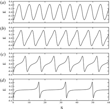
Numerical solution of the normalized electric field for the parameters
 $M=3.5$
,
 ${\it\theta}=2^{\circ }$
,
 $R=10.0$
,
 ${\it\delta}_{c}={\it\delta}_{h}=0.0$
,
 $n_{ec0}/n_{0}=n_{pc0}/n_{0}=0.5$
,
 $T_{c}/T_{h}=0.0$
, and
 $E_{0}=$
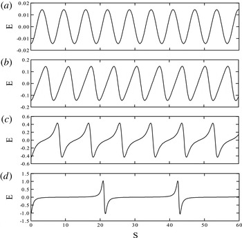
(a) 0.05 (linear waveform), (b) 0.5 (sinusoidal waveform), (c) 1.5 (sawtooth waveform) and (d) 3.5 (bipolar waveform).

Figure 1(a–d) shows the evolution of the system for various driving electric field amplitudes
 $E_{0}$
. The fixed parameters are
 $M=3.5$
,
 $R=10.0$
,
 ${\it\theta}=2^{\circ }$
,
 ${\it\delta}_{c}={\it\delta}_{h}=0.0$
,
 $n_{ec0}/n_{0}=n_{pc0}/n_{0}=0.5$
and
 $T_{c}/T_{h}=0.0$
. Note that wave propagation is taken almost parallel to the ambient magnetic field
 $\boldsymbol{B}_{0}$
. As
 $E_{0}$
increases, the electric field structure evolves from a sinusoidal wave to a sawtooth structure. For a higher
 $E_{0}$
value of 3.5, the potential structure has a spiky bipolar form. As
 $E_{0}$
increases, the period of the wave increases and the frequency decreases. The period of oscillations is given by
 ${\rm\Delta}S=({\rm\Delta}x-V{\rm\Delta}t)({\it\Omega}/V)$
. Typically for
 ${\rm\Delta}x=0$
,
 ${\rm\Delta}S=|{\it\Omega}{\rm\Delta}t|$
. Hence for the linear wave in figure 1(a), with a small driving amplitude of
 $E_{0}=0.05$
, the period of the wave is calculated to be
 $T_{w}=0.995{\it\tau}_{c}$
(frequency
 $f_{w}=1.0f_{c}$
), displaying the cyclotron mode, where
 ${\it\tau}_{c}=2{\rm\pi}/{\it\Omega}$
. In figure 1(b), for
 $E_{0}=0.5$
,
 $T_{w}=1.12{\it\tau}_{c}$
(frequency
 $f_{w}=0.89f_{c}$
). Figure 1(c) shows a sawtooth waveform for
 $E_{0}=1.5$
, with the period of the wave being
 $T_{w}=1.53{\it\tau}_{c}$
(frequency
 $f_{w}=0.66f_{c}$
). For
 $E_{0}=3.5$
(figure 1
d), a spiky bipolar waveform is shown, where the period of the wave is
 $T_{w}=2.62{\it\tau}_{c}$
(frequency
 $f_{w}=0.38f_{c}$
). It is noted that the period of the spiky structure is about two and a half times the cyclotron period and is consistent with the associated acoustic mode.
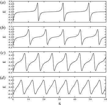
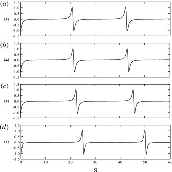
Figure 2(a–d) shows the effect of the Mach number on the electrostatic waves. Here
 $M$
is varied from 3.0 to 5.0 with the fixed parameters,
 $E_{0}=2.0$
,
 $R=10.0$
,
 ${\it\theta}=2^{\circ }$
,
 ${\it\delta}_{c}={\it\delta}_{h}=0.0$
,
 $n_{ec0}/n_{0}=n_{pc0}/n_{0}=0.5$
and
 $T_{c}/T_{h}=0.0$
. As the Mach number increases, the wave structure changes from a sharp spiky form to a more sawtooth-like form. This indicates that the level of nonlinearity decreases with increasing
 $M$
given the sequence observed when
 $E_{0}$
is increased in figure 1(a–d). A similar behaviour of the structures going from spiky to becoming sinusoidal with increasing Mach number is also found by Lu et al. (Reference Lu, Liu, Wang, Stenflo, Popel and Yu2010) for e–p plasma (see figures 2 and 3 of their paper). Hence for larger values of
 $M$
, a stronger
 $E_{0}$
is required to generate the spiky structures. Also noted is that the period of the wave decreases with an increase in the Mach number. For
 $M=3.0$
, which is the minimum value for which a periodic nonlinear waveform exists for the above fixed parameters, the wave has a period of
 $T_{w}=2.62{\it\tau}_{c}$
(frequency
 $f_{w}=0.38f_{c}$
), implying an associated driven acoustic mode. As the Mach number increases to 5.0, the period of the wave decreases to
 $1.15{\it\tau}_{c}$
(frequency
 $f_{w}=0.87f_{c}$
), exhibiting a sawtooth type structure.
Numerical solution of the normalized electric field for the parameters
 $E_{0}=2.0$
,
 $R=10.0$
,
 ${\it\theta}=2^{\circ }$
,
 ${\it\delta}_{c}={\it\delta}_{h}=0.0$
,
 $n_{ec0}/n_{0}=n_{pc0}/n_{0}=0.5$
,
 $T_{c}/T_{h}=0.0$
, and
 $M=$
(a) 3.0, (b) 3.5, (c) 4.0 and (d) 5.0.

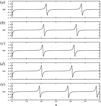
The effect of the drift velocities for the hot electron and positron components are shown in figure 3(a–e). The fixed parameters are
 $E_{0}=3.5$
,
 $M=3.5$
,
 $R=10.0$
,
 ${\it\theta}=2^{\circ }$
,
 ${\it\delta}_{c}=0.0$
,
 $n_{ec0}/n_{0}=n_{pc0}/n_{0}=0.5$
and
 $T_{c}/T_{h}=0.0$
. The period of the spiky structures decreases from
 $3.83{\it\tau}_{c}$
for
 ${\it\delta}_{c}=-0.3$
to
 $3.06{\it\tau}_{c}$
for
 ${\it\delta}_{c}=+0.3$
. Here the hot electron and positron flow anti-parallel (parallel) to
 $\boldsymbol{B}_{0}$
increases (decreases) the period of the spiky structure. Previous studies on electron–ion plasmas showed a similar behaviour for the hot electron drift velocities (Reddy et al.
Reference Reddy, Lakhina, Singh and Bharuthram2002; Moolla et al.
Reference Moolla, Bharuthram, Singh and Lakhina2003). For the ESWs observed in the Earth’s magnetosphere, it was found that the period of the ESWs changed rapidly (Kojima et al.
Reference Kojima, Matsumoto, Miyatake, Nagano, Fujita, Frank, Mukai, Paterson, Saito and Machida1994). Given the above found dependence of the periodicity on the hot electron drift speed, it has been suggested that the observed rapid changes in the period of the ESWs could be due to electrons being accelerated in bursts (Moolla et al.
Reference Moolla, Bharuthram, Singh and Lakhina2003). Our results show that a similar phenomenon could occur in an e–p plasma where, due to the symmetry of the system, both species (electrons and positrons) are drifting.
Numerical solution of the normalized electric field for the parameters
 $M=3.5$
,
 $E_{0}=3.5$
,
 $R=10.0$
,
 ${\it\theta}=2^{\circ }$
,
 $n_{ec0}/n_{0}=n_{pc0}/n_{0}=0.5$
,
 $T_{c}/T_{h}=0.0$
,
 ${\it\delta}_{c}=0$
and
 ${\it\delta}_{h}=$
(a)
 $-0.3$
, (b)
 $-0.1$
, (c) 0.0, (d) 0.1 and (e) 0.3.

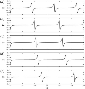
Figure 4(a–e) show the variation of the drift velocities for the cool electron and positron components. The fixed parameters are
 $E_{0}=3.5$
,
 $M=3.5$
,
 $R=10.0$
,
 ${\it\theta}=2^{\circ }$
,
 ${\it\delta}_{h}=0.0$
,
 $n_{ec0}/n_{0}=n_{pc0}/n_{0}=0.5$
and
 $T_{c}/T_{h}=0.0$
. Here we observe that the period of the spiky structures increases from
 $2.89{\it\tau}_{c}$
for
 ${\it\delta}_{c}=-0.3$
, to
 $4.17{\it\tau}_{c}$
for
 ${\it\delta}_{c}=+0.3$
, i.e. as the cool beam flow becomes more parallel to the ambient magnetic field. Therefore, for anti-parallel flow to
 $\boldsymbol{B}_{0}$
, the period of the spiky structure for the cool electrons and positrons decrease and for parallel flow it increases. It is noted that the effect of the cool electron and positron drift velocity on the ESWs is opposite to that compared to the hot electron and positron drift velocity on the waves, indicating that the period of the ESWs depends only on the relative velocity between the cool and hot species.
Numerical solution of the normalized electric field for the parameters
 $M=3.5$
,
 $E_{0}=3.5$
,
 $R=10.0$
,
 ${\it\theta}=2^{\circ }$
,
 $n_{ec0}/n_{0}=n_{pc0}/n_{0}=0.5$
,
 $T_{c}/T_{h}=0.0$
,
 ${\it\delta}_{h}=0$
and
 ${\it\delta}_{c}=$
(a)
 $-0.3$
, (b)
 $-0.1$
, (c) 0.0, (d) 0.1 and (e) 0.3.

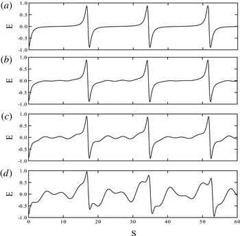
Figure 5(a–d) show the effect of the electron and positron densities on the normalized electric field. The fixed parameters are,
 $E_{0}=1.5$
,
 $M=3.5$
,
 $R=10.0$
,
 ${\it\theta}=2^{\circ }$
,
 ${\it\delta}_{c}={\it\delta}_{h}=0.0$
and
 $T_{c}/T_{h}=0.0$
. As the densities
 $n_{eco}$
and
 $n_{pco}$
increase, the oscillations becomes more nonlinear, with increasing periodicity. With
 $n_{eco}=n_{pco}=0.1$
, a linear waveform of period 1.01
 ${\it\tau}_{c}$
(frequency
 $f_{w}=0.99f_{c}$
) is observed. As the densities are increased (
 $n_{eco}=n_{pco}=0.4$
), the waveform tends to a sawtooth structure of period 1.22
 ${\it\tau}_{c}$
(frequency
 $f_{w}=0.82f_{c}$
). For even larger densities (
 $n_{eco}=n_{pco}=0.7$
), the electric field evolves into a spiky structure of period 2.66
 ${\it\tau}_{c}$
(frequency
 $f_{w}=0.38f_{c}$
). It is noted that a smaller driving electric field is required to drive the nonlinearity of the wave for larger density values. Since the periods of the waves are greater than 1.0
 ${\it\tau}_{c}$
, these waves are associated with a driven acoustic mode.
Numerical solution of the normalized electric field for the parameters
 $M=3.5$
,
 $E_{0}=1.5$
,
 $R=10.0$
,
 ${\it\theta}=2^{\circ }$
,
 ${\it\delta}_{c}={\it\delta}_{h}=0.0$
,
 $T_{c}/T_{h}=0.0$
, and
 $n_{ec0}/n_{0}=n_{pc0}/n_{0}=$
(a) 0.1, (b) 0.3, (c) 0.5 and (d) 0.7.

In figure 6(a–d) we examine the effect of the cool-to-hot electron and positron temperature ratio on the waves. The fixed parameters are,
 $E_{0}=3.5$
,
 $M=3.5$
,
 $R=10.0$
,
 ${\it\theta}=2^{\circ }$
,
 ${\it\delta}_{c}={\it\delta}_{h}=0.0$
and
 $n_{ec0}/n_{0}=n_{pc0}/n_{0}=0.5$
. Here the periodicity and nonlinearity of the wave increases with an increase in the cool-to-hot temperature ratio. The period of the wave increases from 3.42
 ${\it\tau}_{c}$
(frequency
 $f_{w}=0.29f_{c}$
) for
 $T_{c}/T_{h}=0.0$
to 4.02
 ${\it\tau}_{c}$
(frequency
 $f_{w}=0.25f_{c}$
) for
 $T_{c}/T_{h}=0.75$
. This effect may be seen from the linear dispersion relation (2.11), where as the temperature increases,
 ${\it\omega}$
decreases and hence the period of the wave increases.
Numerical solution of the normalized electric field for the parameters with
 $M=3.5$
,
 $E_{0}=3.5$
,
 $R=10.0$
,
 ${\it\theta}=2^{\circ }$
,
 ${\it\delta}_{c}={\it\delta}_{h}=0.0$
,
 $n_{ec0}/n_{0}=n_{pc0}/n_{0}=0.5$
, and
 $T_{c}/T_{h}=$
(a) 0.0, (b) 0.25, (c) 0.5 and (d) 0.75.

In figure 7(a–d), we have varied the propagation angle
 ${\it\theta}$
. The fixed parameters are
 $E_{0}=3.5$
,
 $M=3.5$
,
 $R=10.0$
,
 ${\it\delta}_{c}={\it\delta}_{h}=0.0$
,
 $n_{ec0}/n_{0}=n_{pc0}/n_{0}=0.5$
and
 $T_{c}/T_{h}=0.0$
. The oscillations are of a spiky nature and the periodicity of the wave remains unchanged with a period of
 $2.75{\it\tau}_{c}$
(frequency
 $f_{w}=0.36f_{c}$
), representing an associated acoustic mode. As the propagation angle increases with respect to
 $\boldsymbol{B}_{0}$
, the wave becomes increasingly more distorted with a double-humped feature. The maximum propagation angle that produced a reasonably periodic waveform of this type was found to be
 $35^{\circ }$
.
Numerical solution of the normalized electric field for the parameters
 $M=3.5$
,
 $E_{0}=3.5$
,
 $R=10.0$
,
 $n_{ec0}/n_{0}=n_{pc0}/n_{0}=0.5$
,
 ${\it\delta}_{c}={\it\delta}_{h}=0.0$
,
 $T_{c}/T_{h}=0.0$
, and
 ${\it\theta}=$
(a)
 $2^{\circ }$
, (b)
 $10^{\circ }$
, (c)
 $20^{\circ }$
, (d)
 $35^{\circ }$
.

An examination of the critical driving electric field amplitudes for the onset of spiky electrostatic waves as a function of the Mach number for various density ratio values was conducted for the fixed parameters
 $R=10.0$
,
 ${\it\delta}_{c}={\it\delta}_{h}=0.0$
,
 $T_{c}/T_{h}=0.0$
and
 ${\it\theta}=2^{\circ }$
. It is noted that as the Mach number increases, a larger driving electric field amplitude is required for the onset of the spiky electrostatic waves. The increase of
 $E_{0}$
with
 $M$
is much sharper for lower values of
 $n_{ec0}\;(=n_{pc0})$
. Also as the density ratio increases for a fixed Mach number, the critical driving electric field amplitude for the onset of spiky ESWs decreases. Further, with an increase in the density ratio, the minimum value required for the wave speed decreases for the onset of spiky ESWs.
An examination of the period and pulse width of the electrostatic wave as a function of the drift velocities for the cold electron and positron components (
 ${\it\delta}_{c}$
) was also conducted for the fixed parameters
 $M=3.5$
,
 $E_{0}=3.5$
,
 $R=10.0$
,
 $n_{ec0}/n_{0}=n_{pc0}/n_{0}=0.5$
,
 ${\it\delta}_{h}=0.0$
,
 $T_{c}/T_{h}=0.0$
and
 ${\it\theta}=2^{\circ }$
. It is noted that as the drift velocities for the cold electron and positron component goes from anti-parallel to parallel flow, the period and pulse width of the ESWs increases. This effect is opposite for the drift velocities of the hot electron and positron components, i.e. as you go from anti-parallel to parallel for the hot drift velocities
 ${\it\delta}_{h}$
, the period and pulse width decrease. Similar behaviour from satellite observations was reported, i.e. the period and pulse width decreased (Kojima et al.
Reference Kojima, Matsumoto, Miyatake, Nagano, Fujita, Frank, Mukai, Paterson, Saito and Machida1994). In their measurements, they found that the ratio
 $w/T$
was a constant for the ESWs, with
 $w/T=0.3$
, where
 $w$
is the pulse width and
 $T$
is the period of the wave. In our studies, we found that the ratio
 $w/T$
was also a constant, with
 $w/T\approx 0.96$
.
4 Discussion
In this paper, we have investigated the evolution of nonlinear electrostatic solitary waves in a two-temperature magnetized e–p plasma. In the model considered, spatial variation is restricted to the
 $x$
-direction, while the external magnetic field is in the
 $(x,z)$
plane. In the nonlinear analysis, the associated cyclotron wave and acoustic wave are coupled through the convective derivative terms
 $v_{jx}(\partial v_{jy}/\partial x)$
and
 $v_{jx}(\partial v_{jz}/\partial x)$
in the momentum equations. These two modes are decoupled in the linear analysis. A transition from linear sinusoidal to sawtooth to spiky waveforms is observed as the amplitude of the driving electric field increases. The results found here for an e–p plasma are very similar to those found by other researchers for electron–ion plasmas. On the other hand, as the Mach number is increased (figure 2
a–d) the nonlinearity is suppressed to the point where the bipolar ESWs are no longer excited. For the onset of spiky ESWs, it is noted that as the wave speed increases, a larger driving electric field is required. The periods of the waves are found to be affected by the relative drift between the hot and cold electrons and positrons. Also, the onset of nonlinear structures is affected by the density ratio of the cool-to-hot particle species. As the density ratio increases, the critical value for the driving electric field amplitude for the onset of spiky ESWs decreases and the minimum value required for the wave speed for the onset of spiky ESWs also decreases. The ESWs are therefore more easily excited where the cool species dominate. The results further show that ESWs exists for almost parallel propagation, but as the propagation angle increases with respect to the ambient magnetic field
 $\boldsymbol{B}_{0}$
, the signature waveform becomes more distorted, with a double-humped feature. The ratio of the pulse widths and periods (
 $w/T$
) of the electrostatic waves was found to be a constant, which is consistent with experimental observations (Kojima et al.
Reference Kojima, Matsumoto, Miyatake, Nagano, Fujita, Frank, Mukai, Paterson, Saito and Machida1994) and as found for a plasma consisting of cold and hot electrons and ions (Moolla et al.
Reference Moolla, Bharuthram, Singh, Lakhina and Reddy2007). When finite temperature effects are included, an increase in the temperature ratio of the cool-to-hot electrons and positrons causes the broadening out of the waveforms, which variation is associated with an increase in the wave frequency with
 $T_{c}$
. The nonlinear electrostatic spiky structures studied here may have important implications for pulsars radiation and their microstructure. Firstly, these ESW can modulate the pulsar electromagnetic radiation with a periodicity of
 $T_{w}$
(varying from 1 to 5 times the cyclotron period) leading to some microstructures via modulational instabilities (Hasegawa Reference Hasegawa1975; Luo Reference Luo1998). These fine structures could have a constant
 $w/T=0.96$
. Secondly, the ESWs can couple with the electromagnetic waves and produce a new source of pulsar radiation as discussed by Stark et al. (Reference Stark, Diver, da Costa and Laing2007).
Here, we have not included the electromagnetic and relativistic effects in this paper. However, in the non-relativistic plasma case discussed here, these effects are not expected to be important as both the cyclotron and acoustic modes are electrostatic. The general case of the coupling between electrostatic and electromagnetic modes is quite complex and beyond the scope of this paper.
Acknowledgements
G.S.L. thanks the National Academy of Sciences, India for the support under the NASI-Senior Scientist Platinum Jubilee Fellowship.