2. The concepts of spatial averaging

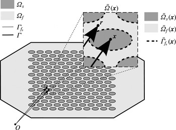
In the context of the spatial averaging technique, a system is regarded as a two- or three-dimensional continuum domain ${\it\Omega}={\it\Omega}_{f}\cup {\it\Omega}_{s}$ which consists of subregions of fluid ( ${\it\Omega}_{f}$ ) and solid ( ${\it\Omega}_{s}$ ) with a common interface boundary ${\it\Gamma}_{fs}$ (figure 1). The solid domain is considered to be composed of solid structures in a periodic configuration. It is assumed that the characteristic size of a single solid structure is small in comparison to the global domain size.

Figure 1.

Two-dimensional system domain, averaging domain and interface boundaries.

A physical quantity ${\it\phi}$  of interest, for instance the temperature $T$ in the system, can be represented as a mathematical distribution over the solid ( $s$ ) and fluid ( $f$ ) regions:

In the same way, material properties such as mass density ${\it\rho}$ , specific heat capacity $c$ and heat conductivity $k$ are mathematical distributions having a different value for the solid and fluid.

Flow quantities such as pressure $p$ , velocity field $\boldsymbol{u}$ , viscous stress field ${\bf\tau}$ and viscosity ${\it\mu}$ have physical meaning on the fluid domain only. They can be represented by mathematical distributions which are defined as zero in the solid region, e.g.

The spatially averaged or ‘macro-scale’ features of a physical quantity are recovered after applying a smoothing operator $\langle \;\rangle _{m}$ on the corresponding distribution ${\it\phi}$ . The superficial spatial average of the distribution, $\langle {\it\phi}\rangle _{m}$ , is defined by the linear convolution of ${\it\phi}$ with a normalized weighting function $m\in C^{\infty }$ having a compact support in ${\it\Omega}$ and satisfying $m(\boldsymbol{x}-\boldsymbol{r})=0$ for $\boldsymbol{r}\notin \bar{{\it\Omega}}(\boldsymbol{x})$ :

Using the notation above, we associate an averaging domain $\bar{{\it\Omega}}$ with each point $\boldsymbol{x}$ of the domain ${\it\Omega}$ , such that $\boldsymbol{x}$ is the geometrical centroid of $\bar{{\it\Omega}}$ (figure 1). Note that the superficial spatial average $\langle {\it\phi}\rangle _{m}$ is evaluated at position $\boldsymbol{x}$ , while the integration is carried out over all points within $\bar{{\it\Omega}}$ having a position vector $\boldsymbol{r}$ . The parts of the averaging domain that match with the fluid and solid regions are denoted $\bar{{\it\Omega}}_{f}$ and $\bar{{\it\Omega}}_{s}$ respectively: $\bar{{\it\Omega}}=\bar{{\it\Omega}}_{f}\cup \bar{{\it\Omega}}_{s}$ .

Often it is of interest to describe the macro-scale level in terms of the intrinsic spatial average of ${\it\phi}$ over the fluid or over the solid region, which are respectively defined as

with ${\it\epsilon}_{fm}\triangleq \langle {\it\gamma}_{f}\rangle _{m}$ and ${\it\epsilon}_{sm}\triangleq \langle {\it\gamma}_{s}\rangle _{m}$ , where the fluid and solid indicators are given by

The spatial averaging technique allows the decomposition of a distribution into a smoothed or macro-scale part over the fluid and solid regions and a deviation part $\widetilde{{\it\phi}}$ :

In order to have a meaningful average and useful decomposition, we require first that variations of the filtered distributions $\langle {\it\phi}\rangle _{m}^{\,f}$ and $\langle {\it\phi}\rangle _{m}^{s}$ within an averaging window $\bar{{\it\Omega}}$ can be neglected, such that the small-scale effects are filtered away: $\langle \langle {\it\phi}\rangle _{m}\rangle _{m}\simeq \langle {\it\phi}\rangle _{m}$ and $\langle \widetilde{{\it\phi}}\rangle _{m}\simeq 0$ . Second, we require that the filter operator $\langle \;\rangle _{m}$ indeed has a smoothing effect so that the filtered distributions $\langle {\it\phi}\rangle _{m}^{\,f}$ and $\langle {\it\phi}\rangle _{m}^{s}$ are truly macro-scale quantities. This means they undergo significant changes (gradients) over a length scale $\mathscr{L}_{{\it\phi}}$ much larger than the spatial scale $\ell _{{\it\phi}}$ over which the original distribution ${\it\phi}$ – and, as a consequence, also the deviation part $\widetilde{{\it\phi}}$ – undergoes significant changes.

It can be shown (Quintard & Whitaker Reference Quintard and Whitaker1994b ) that in order to fulfil both requirements, the characteristic size $r_{m}$ of the averaging window $\bar{{\it\Omega}}$ has to satisfy the scale constraint

This fundamental scale constraint ensures a separation of the micro-scale details (which are present over a length scale $\ell _{{\it\phi}}$ ), represented by $\widetilde{{\it\phi}}$ , and the filtered or macro-scale quantity $\langle {\it\phi}\rangle _{m}$ (i.e. the average behaviour of the physical quantity with gradients over a length scale $\mathscr{L}_{{\it\phi}}$ ).

In the theory of mathematical distributions, the governing equations for the solid and fluid temperature are formulated with the aid of the time derivative in the usual sense and the gradient in the usual sense, which are defined as

The gradient in the usual sense has to be distinguished from the gradient in the sense of a distribution (Gagnon Reference Gagnon1970; Schwartz Reference Schwartz1978), which is

In the last equation ${\it\delta}_{fs}$ is the Dirac distribution associated with the fluid–solid interface ${\it\Gamma}_{fs}$ . The unit normal vector $\boldsymbol{n}_{fs}$ at the fluid–solid interface ${\it\Gamma}_{fs}$ points from the $f$ -region toward the $s$ -region.

Finally, we provide the following essential theorem (Quintard & Whitaker Reference Quintard and Whitaker1994b ) for the spatial averaging technique:

This spatial averaging gradient theorem shows that when the gradient (in the usual sense) of a distribution is filtered, the result consists of a gradient of the filtered distribution and an additional surface term related to the presence of discontinuities of the distribution at the solid–fluid interface.

In the remainder of this paper, the context should make clear on which weighting function the filter operators $\langle \;\rangle _{m}$ , $\langle \;\rangle _{m}^{\,f}$ and $\langle \;\rangle _{m}^{s}$ are based. The weighting function $m_{V}$ for volume averaging is defined by

In the case when $m=m_{V}$ is chosen, the index $m$ is dropped, so that the intrinsic volume averaging operator, for instance, is represented by $\langle \;\rangle ^{\,f}$ .

3. Spatially averaged temperature equations

When the temperature field and material properties are represented by generalized distributions as in (2.1), the thermal energy equation for the incompressible fluid and solid is written in compact form as

The volumetric heat source in the thermal energy equation is given the symbol $\dot{q}$ , while the viscous dissipation term is given by

In the fluid region, (3.1) takes the form

while in the solid region, the equation becomes

The temperature distribution $T$ over the solid and fluid satisfies two constraints at the fluid–solid interface. First, the temperature must be continuous at the fluid–solid interface:

Second, because the energy transfer at the fluid–solid interface is solely due to thermal conduction, the temperature at the interface maintains a continuous interfacial heat flux $q_{fs}$ from the fluid to the solid, so by Fourier’s law:

In the generalized form of (3.1), the temperature equation can be spatially smoothed over the entire system domain ${\it\Omega}$ . After multiplying (3.1) with ${\it\gamma}_{f}$ , using the spatial decomposition of (2.6) and the gradient theorem (2.10), we find the following equation for the macro-scale temperature of the fluid in ${\it\Omega}$ :

with $\boldsymbol{D}\triangleq \langle \boldsymbol{u}T\rangle _{m}-{\it\epsilon}_{fm}\langle \boldsymbol{u}\rangle _{m}^{f}\langle T\rangle _{m}^{f}$ .

The equation for the macro-scale solid temperature $\left\langle T\right\rangle _{m}^{s}$ is

This last equation is directly obtained by multiplying (3.1) with ${\it\gamma}_{s}$ and taking the weighted spatial average.

One should be aware that the macro-scale temperature equations (3.7) and (3.8) are derived under the assumption that the specific heat capacities and conductivities of fluid and solid are quasi-spatially constant over the local averaging domains $\bar{{\it\Omega}}_{f}$ and $\bar{{\it\Omega}}_{s}$ . Although a complete derivation is omitted here, we remark that the necessary steps are very similar to those in the volume-averaging procedure, discussed by e.g. Quintard & Whitaker (Reference Quintard, Whitaker, Vadai and Hadim2000) and Leroy, Goyeau & Taine (Reference Leroy, Goyeau and Taine2013).

The macro-scale temperature equations (3.7) and (3.8) contain three closure terms, involving the micro-scale temperature effects. The first closure term is the weighted interfacial heat transfer,

which is the heat transfer by conduction from fluid to solid at the solid–fluid interface contained within the averaging domain. The interfacial heat transfer term defines the heat transfer coefficient $h_{fs}$ .

The second closure term is given by

and is called the weighted thermal tortuosity. The thermal tortuosity represents the effect at the macro-scale level of heat transfer by conduction at the fluid–solid interface due the fact that this interface forms a tortuous flow path and heat transfer surface.

The third closure term, denoted by $\boldsymbol{D}$ in (3.7), is the weighted thermal dispersion source,

Thermal dispersion is the heat transfer due to hydrodynamic mixing of the fluid at the micro-scale level, thus the convective spreading of heat caused by local variations in fluid velocity about the macro-scale flow. Thermal dispersion is represented by means of the dispersion vector $\boldsymbol{k}_{d}$ . The approximations $\boldsymbol{D}\simeq \langle \widetilde{\boldsymbol{u}}\widetilde{T}\rangle _{m}$ and $\boldsymbol{k}_{d}\simeq \boldsymbol{k}_{d,approx}$ are valid as long as the filter window is small in comparison to the characteristic length scale over which the filtered temperature and filtered velocity change:

because $\langle \widetilde{\boldsymbol{u}}\rangle _{m}\simeq 0$ and $\langle \widetilde{T}\rangle _{m}\simeq 0$ in that case.

It must be emphasized that (3.7) and (3.8) can be justifiably called macro-scale equations if the filtered temperature and filtered velocity satisfy the length scale requirements for spatial smoothing:

By choosing the weighting function $m$ and size $r_{m}$ of the averaging window so as to satisfy (3.13), the macro-scale temperature and velocity fields will vary over length scales $\mathscr{L}_{T}$ and $\mathscr{L}_{\boldsymbol{u}}$ larger than the scales $\ell _{T}$ and $\ell _{\boldsymbol{u}}$ over which the non-smoothed temperature and velocity fields change. As a consequence, the macro-scale temperature equations can be discretized and solved on a coarser mesh than the one needed for a direct numerical simulation of $T$ through (3.3) and (3.4). This consequence can also be understood by noting that the mesh no longer has to capture the small-scale temperature deviation $\widetilde{T}$ , related to geometric intricacies of the solid–fluid interface over the entire fluid domain. The use of a coarser mesh beneficially translates into a reduction of computational effort.

4. Global closure of the spatially averaged temperature equations

The macro-scale temperature equations cannot be directly solved for some prescribed boundary conditions, since the three closure terms are still unknown. For the calculation of the closure terms, knowledge of the full temperature distribution $T$ is required, which includes both the macro-scale temperatures $\langle T\rangle _{m}^{\,f}$ and $\langle T\rangle _{m}^{s}$ as well as the deviation field $\widetilde{T}$ . Hence, the relation between the unknown closure terms and the macro-scale temperatures of fluid and solid has to be sought by solving the following global closure problem for the fluid deviation temperature $\widetilde{T}_{f}$ :

and the following closure problem for the solid deviation temperature $\widetilde{T}_{s}$ :

This system of equations for the deviation quantities $\widetilde{T}_{f}$ and $\widetilde{T}_{s}$ is obtained by subtracting the spatially averaged temperature equations (3.7) and (3.8) from the original thermal energy equation (3.1), in the $f$ - and $s$ -regions. The term ${\it\psi}_{m}^{\prime }$ collects all additional contributions which arise in the closure problem when $\boldsymbol{{\rm\nabla}}{\it\epsilon}_{fm}\neq 0$ and $\boldsymbol{{\rm\nabla}}{\it\epsilon}_{sm}\neq 0$ . It is defined as

where $\boldsymbol{D}^{\prime }\triangleq {\it\epsilon}_{fm}^{-1}\boldsymbol{D}\simeq \langle \widetilde{\boldsymbol{u}}\widetilde{T}\rangle _{m}^{\,f}$ .

Because the closure equations contain all small-scale features $\widetilde{T}_{f}$ and $\widetilde{T}_{s}$ throughout the whole system domain, their solution requires the same mesh resolution as needed for solving the original thermal problem. Hence, the closure equations are very expensive to solve. Moreover, there is a complex coupling between the closure problems and the smoothed macro-scale equations: the macro-scale temperatures and deviation temperatures need to be solved simultaneously in order to resolve the coupling closure terms.

Without any additional assumptions, the determination of the closure terms thus requires even more computational effort than solving the original temperature equations. However, in the remaining sections we will derive a simplified closure strategy which yields the closure terms for the periodically developed heat transfer regime in the case where the solid temperature is constant. The next section first explores the mathematical description of the periodically developed heat transfer regime in isothermal solid structures.

5. Periodically developed heat transfer in isothermal solids

The appropriate definition of the periodically developed heat transfer regime is that there exists a periodic similarity in the temperature distribution over some part of the domain as a result of the periodically developed flow field in that part of the domain. For a system domain composed of periodic solid structures, this periodic similarity implies that the profiles of the temperature distribution contained within different unit cells of the solid structures can be brought together by a suitable mathematical transformation or scaling.

Here a unit cell is defined as a local domain spanned by three lattice vectors $\boldsymbol{l}^{(j)}$ :

where the three lattice vectors are defined through the periodicity of the fluid and solid indicators for any position $\boldsymbol{x}$ sufficiently far from the external boundaries of the domain ${\it\Omega}$ :

In the case where the solid structures have a temperature $T_{s}$ which is constant over the solid domain and no viscous dissipation nor volumetric heat generation occurs, we can seek a suitable temperature scaling for the steady periodically developed heat transfer regime by adopting the transformation of Patankar et al. (Reference Patankar, Liu and Sparrow1977) for periodic heat transfer in ducts with uniform wall temperature. Accordingly, we introduce the rescaled temperature

where $T_{ref}$ is a local reference temperature yet to be determined.

For steady periodically developed flow, the flow field varies in a periodic fashion from one unit cell to another:

Therefore, we postulate the existence of a suitable reference temperature $T_{ref}$ such that the temperature transformation of (5.3) yields a periodic steady-state rescaled temperature which is similar for every unit cell:

The occurrence of the periodic similarity in the temperature distribution expressed by (5.5) thus serves as a definition for the steady periodically developed heat transfer regime when the solid temperature is constant.

If the rescaled temperature ${\it\theta}$ is substituted into the temperature equation (3.1), the following equation results:

where

and

As we look for a steady solution and assume that there are no temperature changes due to viscous dissipation and volumetric heat sources, the corresponding terms in (5.6) and (5.7) are zero:

Mathematically, a steady periodic solution for ${\it\theta}$ by (5.6) is possible under the condition that the fluid properties are space independent and the local reference temperature satisfies

as in that case the source term in the rescaled temperature equation is also periodic:

Because ${\it\theta}_{s}=0$ , it suffices to determine ${\it\theta}_{f}$ by resolving (5.6) on the fluid domain of the unit cell. The appropriate boundary conditions for ${\it\theta}_{f}$ in ${\it\Omega}_{f}\cap {\it\Omega}_{unit}$ are thus

In the periodically developed regime for isothermal solids, the rescaled temperature depends on the constant fluid properties, the velocity field and ${\bf\lambda}_{T}$ via (5.6) as well as the unit cell geometry via (5.12):

When the flow is steady and periodically developed, it can be shown (Buckinx & Baelmans Reference Buckinx and Baelmans2015) that the functional dependence of the velocity field is given by the following parameter set:

where $\boldsymbol{f}$ represents a spatially periodic body force over the unit cell domain. In conclusion, by (5.13) it holds that

6. Choice of reference temperature

If a suitable reference temperature can be found which satisfies (5.10), ${\it\theta}$ represents a periodic similarity between the temperature profiles within different unit cells. For periodically developed heat transfer in ducts with streamwise-periodic variations of cross-sectional area, Patankar et al. (Reference Patankar, Liu and Sparrow1977) suggested that any temperature in the local cross-section of the duct could be chosen as $T_{ref}$ in order to have periodicity of ${\it\theta}$ .

For the periodically developed heat transfer regime in solid structures, one can also make use of a cross-sectional reference temperature, at least if the flow has a main direction which coincides with one of the lattice vectors. Suppose the main flow is directed along $\boldsymbol{l}^{(k)}$ ; a convenient choice of cross-sectional reference temperature could be the modified bulk temperature $T_{b}$ , which is defined by

and based on the local cross-section perpendicular to $\boldsymbol{l}^{(k)}$ ,

As shown by Patankar et al. (Reference Patankar, Liu and Sparrow1977), ${\bf\lambda}_{T}$ will not be constant over space if $T_{ref}=T_{b}$ .

While the choice of a cross-sectional reference temperature seems suited to flow through ducts, it might not be for flow through periodic solid structures. First, it is not straightforward to identify an appropriate local cross-section for a periodic solid structure if the main flow is not aligned with one of the lattice vectors. Second, with the aim of simplifying the rescaled temperature equation (5.6), it is more interesting to choose a reference temperature such that ${\bf\lambda}_{T}$ is a spatially constant vector,

For that reason we propose

This reference temperature represents, apart from the offset $T_{s}$ , the exponential envelope of the physical temperature $T$ , for which ${\it\theta}$ acts like a modulated carrier signal. The same form of reference temperature was also used by Stalio & Piller (Reference Stalio and Piller2006) in their study of unsteady periodic flow and heat transfer in converging–diverging wavy channels.

Any reference temperature of the form

with

will also lead to a periodic rescaled temperature ${\it\theta}$ and to a constant temperature ratio over the unit cell (Nakayama et al. Reference Nakayama, Kuwahara and Hayashi2004; Teruel & Díaz Reference Teruel and Díaz2013),

However, for any reference temperature different from (6.4), ${\bf\lambda}_{T}(\boldsymbol{x})$ will always vary periodically over space.

If one opts for a filtered temperature as reference, i.e.

the appropriate weighting function $m$ should be constructed such that ${\it\theta}$ and ${\bf\lambda}_{T}$ can be made periodic. This is, for instance, the case if $m=m_{V}$ or $m=m_{V}\ast m_{V}$ and the filter window of $m_{V}$ matches with a unit cell of the domain, $\bar{{\it\Omega}}={\it\Omega}_{unit}$ in (2.11). In § 8, we will derive the weighting function $m$ for which ${\bf\lambda}_{T}$ and hence ${\it\tau}_{T}^{(j)}$ are constant.

7. Reference temperature eigenvalue problem

When the decay rate of the reference temperature ${\bf\lambda}_{T}$ is constant over space, its value can be governed by averaging the steady form of (5.6) under absence of heat sources:

with

because ${\bf\lambda}_{T}$ is assumed constant over space. Note that in (7.1), we made use of the equality ${\it\theta}_{f}=0$ at ${\it\Gamma}_{fs}$ , because $T_{f}=T_{s}$ at the fluid–solid interface according to (3.5).

If one chooses a weighting function of the form $m=m_{G}\ast m_{V}$ , where $m_{G}$ is an arbitrary weighting function and the filter window of $m_{V}$ matches a unit cell of the domain, i.e. $\bar{{\it\Omega}}={\it\Omega}_{unit}$ , all the weighted averages of periodic terms in (7.1) reduce to their constant volume-averaged value. Hence, if $m=m_{G}\ast m_{V}$ , (7.1) and (7.2) reduce to a quadratic equation for the temperature decay rate:

From physical considerations, only the negative decay rate ${\it\lambda}_{T}<0$ of (7.3) makes sense. Because $\langle \boldsymbol{u}\rangle _{m}=\langle \boldsymbol{u}\rangle =\Vert \langle \boldsymbol{u}\rangle \Vert \boldsymbol{e}_{s}$ is a constant vector when $m=m_{G}\ast m_{V}$ , the reference temperature must decay exponentially in the main flow direction, so $\boldsymbol{e}_{{\it\lambda}}=\boldsymbol{e}_{s}$ . Moreover, (7.3) shows that the decay rate only determines the rescaled temperature up to an arbitrary constant, so that its volume-average can be set to

In fact, (7.3) might be called the eigenvalue problem for periodically developed heat transfer in isothermal solid structures, as it resembles an analogue of the eigenvalue problem for the fluid bulk temperature in fully developed heat transfer in ducts with constant wall temperature (Shah & London Reference Shah and London1978).

In summary, when ${\bf\lambda}_{T}$ is constant, its value corresponds to the negative root of (7.3), which is directly determined by the velocity field $\boldsymbol{u}$ and rescaled temperature ${\it\theta}$ within the unit cell. Therefore, the decay rate ${\bf\lambda}_{T}$ can be left out of the functional relationship (5.15):

Consequently, the decay rate itself depends on the fluid properties, the volume-averaged velocity and the geometry of the unit cell domain:

8. Choice of weighting function

Up to this point, the question of how to choose the weighting function for the spatially averaged temperature has been left unanswered. Nevertheless, in the previous sections several restrictions have been imposed on the weighting function. First of all, the weighting function is required to be normalized and infinitely derivable. Second, the weighting function should respect the length scale constraints for spatial smoothing in (3.13).

Let us again propose a weighting function of the form $m=m_{G}\ast m_{V}$ , where the filter window of $m_{V}$ matches a unit cell of the domain, $\bar{{\it\Omega}}={\it\Omega}_{unit}$ . This weighting function $m$ satisfies

for any spatially periodic distribution ${\it\phi}$ .

Consequently, if $m=m_{G}\ast m_{V}$ , the weighted porosity equals the constant physical porosity or void fraction, ${\it\epsilon}_{fm}={\it\epsilon}_{f}\triangleq \langle {\it\gamma}_{f}\rangle$ . By (5.4), this weighting function also yields a spatially constant filtered velocity $\langle \boldsymbol{u}\rangle _{m}^{\,f}=\langle \boldsymbol{u}\rangle ^{\,f}$ for periodically developed flow. Hence, the weighting function $m$ respects the velocity scale constraint of (3.13), as it leads to the order of magnitude estimates $\ell _{\boldsymbol{u}}\leqslant r_{m}=O(\Vert \boldsymbol{l}^{(j)}\Vert )$ and $\mathscr{L}_{\boldsymbol{u}}=\infty$ .

In order that $m=m_{G}\ast m_{V}$ would also satisfy the temperature scale constraint of (3.13), we will choose $m_{G}$ in a manner such that for the overall weighting function $m$ it additionally holds that

where ${\it\phi}$ is any arbitrary distribution and ${\bf\lambda}_{T}$ is the constant temperature decay rate vector given by (6.3). (Note that the expression $\langle {\it\phi}\text{e}^{{\bf\lambda}_{T}\boldsymbol{\cdot }\boldsymbol{r}}\rangle _{m}$ is actually an abuse of notation and should be interpreted as ${\it\phi}(\boldsymbol{r})\text{e}^{{\bf\lambda}_{T}\boldsymbol{\cdot }\boldsymbol{r}}$ appearing as a function of the integration variable $\boldsymbol{r}$ within the integral operator $\langle \;\rangle _{m}$ .)

The above property of the weighting function ensures that the spatially averaged temperature remains unaltered after repeatedly averaging:

The scale constraint $r_{m}\ll \mathscr{L}_{T}$ is then automatically satisfied because $\langle \widetilde{T}\rangle _{m}=0$ by (8.3). The fact that this overall weighting function suppresses the temperature deviation field after filtering can also be seen from the expression

by remarking that $\langle \widetilde{{\it\theta}}\rangle =0$ . As a comment, we add that because the exponential temperature envelope in (8.4) is

${\it\theta}$ plays the role of a closure mapping function for the deviation temperature, as often used in the theory for porous media (Quintard et al. Reference Quintard, Kaviany and Whitaker1997; DeGroot & Straatman Reference DeGroot and Straatman2011).

Furthermore, if the weighting function $m$ is chosen to have the properties of (8.1) and (8.2), the length scale for the filtered temperature can be estimated by $\mathscr{L}_{T}=O({\it\lambda}_{T}^{-1})$ , because

On the other hand, according to (8.4), the length scale for the deviation temperature can be estimated by $\ell _{T}=O\left(\ell _{{\it\theta}}\right)$ . Therefore, the weighting function with the above properties also satisfies $\ell _{T}\ll \mathscr{L}_{T}$ .

It is readily verified that the overall weighting function $m$ satisfying both (8.1) and (8.2) is given by $m=m_{G}\ast m_{V}=m_{C}\ast m_{{\it\lambda}}\ast m_{V}$ , where $m_{C}$ is arbitrary and

The normalization factor ${\it\beta}$ for $m_{{\it\lambda}}$ is derived in appendix A and depends on the temperature decay rate:

with

The appropriate filter operator $\langle \;\rangle _{m}$ for the periodically developed heat transfer regime in isothermal periodic solid structures is thus a matched filter, because its kernel $m=m_{C}\ast m_{{\it\lambda}}\ast m_{V}$ matches the decay rate ${\it\lambda}_{T}$ of the exponentially decreasing temperature envelope. Moreover, if we set $\langle {\it\theta}\rangle =1$ by (7.4), the reference temperature proposed in § 6 is found by averaging the full-scale temperature distribution $T$ with this matched filter:

When the decay rate is sufficiently small, i.e.

the overall weighting function $m=m_{C}\ast m_{{\it\lambda}}\ast m_{V}$ can be approximated as $m\simeq m_{C}\ast m_{V}\ast m_{V}$ , which is the appropriate weighting function for the pressure and velocity in the periodically developed flow regime (Buckinx & Baelmans Reference Buckinx and Baelmans2015). Theoretically, $m_{C}$ should be chosen such that $(m_{C}\ast m_{V}\ast m_{V})\in C^{\infty }$ , because $(m_{V}\ast m_{V})\in C^{0}$ . For numerical purposes one can take $m_{C}\simeq 1$ , as differentiability of the weighting function is seldom of concern. In that case we have for (8.11), $m\simeq m_{V}\ast m_{V}$ or equivalently,

Because $\langle {\it\phi}\rangle _{m}=\langle \langle {\it\phi}\rangle \rangle$ if $m=m_{V}\ast m_{V}$ , the above filter operator is equivalent to a double volume average. This means that, for small eigenvalues of (7.3), the filter need only be customized to the spatial periods of the solid structures, which are determined by the three lattice vectors.

In the limit of (8.11), the double volume filter can be further approximated by a single volume filter, $\langle \langle {\it\phi}\rangle \rangle \simeq \langle {\it\phi}\rangle$ . As the double filtered temperature for any weighting function $m$ is given by the Taylor series

we see that the approximation $\langle \langle T\rangle \rangle \simeq \langle T\rangle$ requires at least that terms involving the volume-averaged spatial moments $\langle (\boldsymbol{r}-\boldsymbol{x})^{\otimes n}\rangle$ are negligible:

The volume-averaged spatial moments $\langle (\boldsymbol{r}-\boldsymbol{x})^{\otimes n}\rangle$ vary periodically over a unit cell of the periodic solid structures. Depending on the type of solid structures, the influence of the spatial moments on the macro-scale temperature might be considerable, so that (8.14) might be violated. Moreover, the validity of (8.14) is difficult to check from an a priori analysis. Therefore, it is recommended to use a double volume filter, i.e. $m=m_{V}\ast m_{V}$ , whenever the temperature decay rate is expected to be small.

9. Closure for periodically developed heat transfer

With the aid of the weighting function $m=m_{C}\ast m_{{\it\lambda}}\ast m_{V}$ , the closure problem of § 4 becomes equivalent to the rescaled temperature equations of § 5 in the periodically developed heat transfer regime. Suitably, the closure problem can be strongly simplified. Indeed, when $\langle {\it\theta}\rangle =1$ and therefore $T_{ref}=\langle T\rangle _{m}$ , the relationship between the closure terms and the macro-scale temperature becomes very simple, as the macro-scale temperature $\langle T\rangle _{m}$ can be moved outside the averaging operator $\langle \;\rangle _{m}$ due to the filter property of (8.2).

The thermal dispersion source, for instance, can be expressed as

if $\langle {\it\theta}\rangle =1$ , by virtue of (8.3), (8.4) and (8.5). Note that $\boldsymbol{D}=\langle \widetilde{\boldsymbol{u}}\widetilde{T}\rangle _{m}$ is exact, because $\langle \widetilde{\boldsymbol{u}}\rangle _{m}=0$ and $\langle \widetilde{T}\rangle _{m}=0$ . Hence, the thermal dispersion vector coefficient is

The interfacial heat transfer term is related to the macro-scale temperature as follows:

where we have used (8.5) and the property ${\it\theta}_{f}=0$ at ${\it\Gamma}_{fs}$ , because of (3.5). Therefore, if $\langle {\it\theta}\rangle =1$ , the convective heat transfer coefficient in periodically developed flow is

Finally, the thermal tortuosity is given by

and hence vanishes for a periodic solid structure as ${\it\epsilon}_{fm}={\it\epsilon}_{f}$ is constant.

From the previous expressions, we conclude that the weighting function $m=m_{C}\ast m_{{\it\lambda}}\ast m_{V}$ allows us to represent the closure terms by means of a spatially constant interfacial heat transfer coefficient and spatially constant dispersion vector, at least for the periodically developed heat transfer regime in periodic solid structures. Both spatially constant closure coefficients follow from the rescaled temperature distribution on a unit cell. Accordingly, the functional dependence of the interfacial heat transfer coefficient is given by

In the absence of a body force and for a fixed flow direction as well as fixed unit cell geometry with characteristic reference length $L_{ref}$ , the above relationship can also be expressed as a dimensionless correlation between the Nusselt number ( $h_{fs}L_{ref}^{2}/k_{f}$ ), the Reynolds number based on the volume-averaged velocity ( ${\it\rho}_{f}\left\Vert \langle \boldsymbol{u}\rangle \right\Vert L_{ref}/{\it\mu}_{f}$ ) and the Prandtl number ( ${\it\mu}_{f}c_{f}/k_{f}$ ). The dispersion vector has a functional dependence similar to that of the interfacial heat transfer coefficient and thus also varies with the Reynolds number and Prandtl number when $m=m_{C}\ast m_{{\it\lambda}}\ast m_{V}$ .

The weighting function $m=m_{C}\ast m_{{\it\lambda}}\ast m_{V}$ imposes the following relationship between the closure coefficients $\boldsymbol{k}_{d}$ and $h_{fs}$ and the temperature decay rate:

This relationship follows from the macro-scale energy equation (3.7) after substitution of the definitions of the closure coefficients and ${\bf\lambda}_{T}$ . Equation (9.7) is completely equivalent to the eigenvalue problem of (7.3). It shows that the rescaled macro-scale temperature gradient ${\bf\lambda}_{T}$ , projected in the direction of the macro-scale flow velocity $\langle \boldsymbol{u}\rangle$ , is caused by an imbalance between macro-scale conduction effects, thermal dispersion and convective macro-scale heat transfer at the fluid–solid interface. Because (9.7) is the only mechanism for inducing a macro-scale temperature gradient, it explains why the vector ${\bf\lambda}_{T}$ has solely a component along the macro-scale flow direction $\boldsymbol{e}_{s}$ in the developed regime.

By (9.7), the negative eigenvalue of the reference temperature or macro-scale temperature decay rate is also given by

In order that ${\it\lambda}_{T}$ be a real negative number, the discriminant of (9.7) must be greater than or equal to zero. Therefore, in order to have at least one physically possible solution, the closure coefficients must satisfy

In the special case when macro-scale conduction effects and thermal dispersion are negligible in (9.7), one finds that the constant exponent of the macro-scale temperature is

This constant exponent was introduced as the decay rate of the volume-averaged temperature in the study of Kuwahara, Shirota & Nakayama (Reference Kuwahara, Shirota and Nakayama2001), Nakayama et al. (Reference Nakayama, Kuwahara, Umemoto and Hayashi2002, Reference Nakayama, Kuwahara and Hayashi2004), although our analysis shows that it requires the macro-scale temperature to be based on the weighting function $m=m_{C}\ast m_{{\it\lambda}}\ast m_{V}$ .

10. Macro-scale heat transfer in an array of isothermal cylinders

In the following case study, the weighted spatial averaging technique is applied to describe the steady macro-scale heat transfer through an array of $N$ solid cylinders at constant temperature. This simple case study provides some illustrations which reveal the main characteristics of the periodically developed heat transfer regime in isothermal periodic solid structures.

Figure 2.

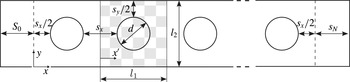
Geometry of cylinder array and unit cell.

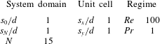
The geometrical parameters of the cylinder array in figure 2 consist of the cylinder diameter $d$ , the horizontal and vertical cylinder spacing $s_{x}$ and $s_{y}$ , as well as the positions of the first and last cylinder, $s_{0}$ and $s_{N}$ respectively. A two-dimensional unit cell of the array with lattice sizes $l_{1}$ and $l_{2}$ and local axis $x^{\prime }$ is indicated by the checker-board pattern in figure 2. The values of all the case study parameters are summarized in table 1.

Table 1.

Case study parameters.

The flow field through the array is considered two-dimensional and the main flow direction is along the $x$ -axis of the global reference frame. The $y$ -axis is therefore perpendicular to the main flow. The total pressure drop ${\rm\Delta}p$ over the array between in- and outlet is specified as a boundary condition. At the boundaries of the solid cylinders, the velocity field satisfies the no-slip condition. Furthermore, the inlet temperature $T_{in}$ is prescribed and a zero gradient condition is set for the temperature at the outlet. At the other domain boundaries, symmetry boundary conditions for the velocity, pressure and temperature distributions are imposed.

For numerically solving the steady Navier–Stokes flow and temperature equations with the finite-volume method, the gradient operator is discretized according to the least-square gradient scheme of Haselbacher & Blazek (Reference Haselbacher and Blazek2000), while the Laplacian operator is discretized using the approach of Traoré, Ahipo & Louste (Reference Traoré, Ahipo and Louste2009). A linear face interpolation scheme is used for the discrete divergence operator. The unstructured finite-volume mesh for the cylinder array consists of a series of $N$ square mesh blocks, each centred around a single cylinder. Every mesh block is composed of a nearly orthogonal elliptic mesh of about 100 000 quadrilateral cells for the fluid region and a triangular Delaunay mesh of about 6000 cells for the cylindrical solid region. The mesh for the solid region is used to apply the discrete spatial filter operator proposed by Buckinx & Baelmans (Reference Buckinx and Baelmans2015) on the discrete flow and temperature distributions.

All distributions in this case study are filtered assuming periodicity over the symmetry boundaries, so that the filtered quantities vary only in the $x$ -direction over the cylinder array. The one-dimensional nature of the filtered results facilitates their graphical representation and interpretation.

Figure 3.

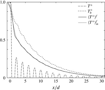
Filtered dimensionless temperature distributions at the centreline $y=l_{2}/2$ of the cylinder array.

Figure 3 presents the dimensionless temperature profile at the centreline of the cylinder array. The dimensionless temperature $T^{+}\triangleq (T-T_{s})/(T_{in}-T_{s})$ is defined such that it becomes zero in the solid domain. Figure 3 shows that the fluid temperature decreases in front of each cylinder, as the bulk fluid transfers heat to the cylinders, which maintain a temperature $T_{s}^{+}=0$ lower than the bulk fluid temperature $T_{b}^{+}$ (cf. (6.1)). In the wake zone after each cylinder, the heat transfer is lower than in front of the cylinder, due to a lower fluid velocity in this region and the existence of a recirculation zone. Therefore, the fluid temperature rises again in the wake zone behind each cylinder.

In this laminar flow regime at a moderate Reynolds number, $\mathit{Re}\triangleq {\it\rho}_{f}U_{ref}d/{\it\mu}_{f}=100$ where $U_{ref}\triangleq \sqrt{{\rm\Delta}p/{\it\rho}_{f}}$ , the flow field is affected by entrance effects only over a short distance from the inlet. As a result, the flow is already periodically developed after the second cylinder. Also, the heat transfer regime is periodically developed downstream from the second cylinder. The simultaneous development of the flow and temperature fields can be explained by noting that the relative scales of momentum diffusion and thermal diffusion are equal in this case: $\mathit{Pr}=1$ .

The onset of the periodically developed heat transfer regime is reflected by the exponentially decreasing profile of the filtered temperature $\langle T^{+}\rangle _{m}^{\,f}$ in figure 3, for $x/d>4$ . The intrinsically filtered temperature $\langle T^{+}\rangle _{m}^{\,f}$ in figure 3 is calculated with the matched weighting function $m=m_{{\it\lambda}}\ast m_{V}$ . In this specific case, the decay rate ${\it\lambda}_{T}$ of the filtered temperature is rather small, ${\it\lambda}_{T}l_{1}\ll 1$ , so that the weighting function $m=m_{V}\ast m_{V}$ would have yielded nearly the same curve for $\langle T^{+}\rangle _{m}^{\,f}$ as the matched filter in figure 3. On the other hand, the difference between the intrinsically volume-averaged temperature $\langle T^{+}\rangle ^{\,f}$ and filtered temperature $\langle T^{+}\rangle _{m}^{\,f}$ is more pronounced. The profile of the volume-averaged temperature wiggles around the profile of $\langle T^{+}\rangle _{m}^{\,f}$ in figure 3, indicating that the decay rate of $\langle T^{+}\rangle ^{\,f}$ in the developed regime varies periodically over the array.

Figure 4.

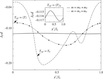
Variation of the decay rate over the unit cell domain for different reference temperatures.

The reference temperature decay rate (cf. (5.8)) in the periodically developed regime is shown in figure 4 for four different reference temperatures $T_{ref}$ over the unit cell domain. The appropriate reference temperature for the periodically developed heat transfer regime is the macro-scale temperature $\langle T\rangle _{m}$ obtained by filtering the temperature with the matched filter $m=m_{{\it\lambda}}\ast m_{V}$ , because this macro-scale temperature has the same constant decay rate as the physical temperature envelope. The reference temperature $T_{ref}=\langle T\rangle _{m}$ with $m=m_{V}\ast m_{V}$ is obtained by volume-averaging the temperature twice. From figure 4 we observe that in this numerical experiment, the physically meaningful constant temperature decay rate can be determined to a good approximation by averaging the temperature distribution twice with a simple volume filter. On the contrary, by applying a single volume-averaging filter, we find a volume-averaged temperature $\langle T\rangle$ with a distinctly spatially varying decay rate. This makes it difficult to assign a physical meaning to the volume-averaged temperature $\langle T\rangle$ in the periodically developed heat transfer regime. Lastly, figure 4 illustrates that also for the same reason the bulk temperature $T_{b}$ complicates the description of the developed regime in periodic isothermal solids.

Figure 5.

Variation of the interfacial heat transfer coefficient over the unit cell domain for different weighting functions.

The value of the interfacial heat transfer coefficient depends in the first place on the weighting function of the filtered temperature (cf. (3.9)). In figure 5, the heat transfer coefficient $h_{fs}$ for the volume-averaged temperature varies clearly in the main flow direction over the unit cell domain. The fact the heat transfer coefficient for the volume-averaged temperature is a function of the position of the averaging window $\bar{{\it\Omega}}(\boldsymbol{x})={\it\Omega}_{unit}(\boldsymbol{x})$ was also remarked on by Teruel & Díaz (Reference Teruel and Díaz2013). Teruel & Díaz (Reference Teruel and Díaz2013) pragmatically suggested using a double averaging procedure in order to obtain a constant $h_{fs}$ . Their pragmatic solution is also justified in this specific case, because the heat transfer coefficient for the double-averaged temperature $\langle T\rangle _{m}$ with $m=m_{V}\ast m_{V}$ in figure 5 deviates by less than a per cent from its mean value. However, as illustrated in figure 5, a truly constant heat transfer coefficient in the periodically developed regime is theoretically only ensured by the matched weighting function $m=m_{{\it\lambda}}\ast m_{V}$ .

Figure 6.

Variation of the streamwise component of the dispersion vector over the unit cell domain for different weighting functions.

The matched weighting function also yields a constant dispersion coefficient in the developed heat transfer regime. The constant dimensionless dispersion coefficient for $m=m_{{\it\lambda}}\ast m_{V}$ can be calculated in two ways, either as $\boldsymbol{k}_{d}^{+}\triangleq \boldsymbol{k}_{d}/U_{ref}$ or as $\boldsymbol{k}_{d,approx}^{+}\triangleq \boldsymbol{k}_{d,approx}/U_{ref}$ , and is shown in figure 6. The equality $\boldsymbol{k}_{d}=\boldsymbol{k}_{d,approx}$ holds exactly because the thermal dispersion $\boldsymbol{D}=\langle \widetilde{\boldsymbol{u}}\widetilde{T}\rangle _{m}$ for this filter. For the volume filter and double volume filter, $\boldsymbol{D}\simeq \langle \widetilde{\boldsymbol{u}}\widetilde{T}\rangle _{m}$ holds only approximately. The difference between $\boldsymbol{k}_{d}$ and $\boldsymbol{k}_{d,approx}$ is mostly ignored in the context of the volume-averaging technique. Figure 6 confirms that the relative discrepancies between $\boldsymbol{k}_{d}$ and $\boldsymbol{k}_{d,approx}$ for $m=m_{V}$ or $m=m_{V}\ast m_{V}$ are at most 1 % in this case. Nevertheless, one should be careful not to generalize the validity of $\boldsymbol{k}_{d}\simeq \boldsymbol{k}_{d,approx}$ to different solid structures or even other flow and heat transfer regimes with a different $\mathit{Re}$ and $\mathit{Pr}$ .

Figure 7.

Comparison of rescaled temperature profiles around the eighth cylinder (solid lines) with unit cell simulation (circle markers).

The final illustration, figure 7, gives the profiles of the rescaled temperature ${\it\theta}$ within the unit cell for which the centroid coincides with the centre of the eighth cylinder. The profiles obtained by DNS of the temperature field equations, cf. (3.1), are in agreement with the profiles found by solving the rescaled temperature equations (5.6) and (5.12) on the unit cell domain. Figure 7 demonstrates that when the reference temperature for the rescaled temperature corresponds to the macro-scale temperature based on the matched weighting function, a perfect reconstruction of the micro-scale temperature field is possible. The reconstruction requires only knowledge of the unit cell geometry, as well as parameters of the flow and heat transfer regime, $\mathit{Pr}$ and $\mathit{Re}$ .