INTRODUCTION
A large part of economic activity occurs in the home. Empirical studies suggest that the value of home (household) production is between 40 and 50% of measured GNP in most industrialized countries.1
See Eisner (1988) and Bonke (1992) for empirical evidence on this. Furthermore, Juster and Stafford (1991) find that a typical married U.S. couple spend 25% of their time working at home while allocating 33% of their time to market activities. Bonke (1995) finds that women allocate as much as 57% and men as much as 21% of their time to home production. Greenwood et al. (1995) document that investment in household capital is larger than investment in market capital.
See also Benhabib et al. (1991); Greenwood and Hercowitz (1991); Baxter and Jermann (1999); and Wrase (2001). Busato and Chiarini (2004) also analyze the role of home production activity in explaining business cycles.
Motivated in part by such successes, the application of stochastic dynamic home production models has been widespread. These models have proliferated despite an obvious weakness; time series on home production do not exist.3
McGrattan et al. (1997) evaluate the impact of fiscal policy; Canova and Ubide (1998) study business-cycle transmission across countries; and Parente et al. (2000) examine the sources of differences in the standard of living across countries. It is possible to obtain spotty data related to home production activities collected through surveys and time-use diaries (see Juster and Stafford (1991)). Gronau and Hamermesh (2006) examine U.S. and Israeli household data on expenditures of time and goods to analyze how education and age affect the goods intensity of household production.
Ingram et al. (IKS, 1997) develop a complementary approach to deal with the problem of unobservable data.4
This approach is not unique to IKS and has recently been widely used in different contexts. For example, employing the IKS approach, Ingram, Kocherlakota, and Savin (1994a, 1994b) back out the productivity shocks and examine their roles in driving business cycles; Baxter and King (1998) back out the realizations of productivity and preference shocks; Smith and Zin (1997) generate realizations of output, consumption, and employment; Blankenau et al. (2001) back out the world real interest rate series; and Beauchemin (2000) generates public capital series. IKS (1994a, 1994b) also apply this methodology to derive productivity shocks.
In this paper, we use the IKS approach to address several open questions regarding the business-cycle properties of the home sector. The first is whether there are similarities in these properties across similar economies. To address this, we document the stylized business-cycle features of home production activities in industrialized countries. Although the Group of Seven (G-7) countries would be the most appropriate set to consider, data limitations require that we restrict attention to Canada, the United States, Germany, and Japan. These economies are similar, of course, in levels of industrialization and have broadly similar business-cycle features in observable data. However, there are some well-known structural differences in their labor markets that might lead to different home sector behavior.5
See Siebert (1997) for a study of structural differences in the labor markets of nine member countries of the Organisation for Economic Co-operation and Development. Genay and Loungani (1997) study the similarities and differences in the cyclical dynamics of labor markets in the United States and Japan. Bertola and Rogerson (1997) analyze the differences in labor markets in Europe and the United States and emphasize the importance of these in explaining the dynamics of unemployment.
Our results suggest that despite these differences, there are some important similarities in the cyclical properties of home sector variables across the countries we consider. For example, we find that home production is more volatile than market production, whereas the volatility of hours spent in home production is close to that of market hours. Leisure is much less volatile than any other series. In addition, home production variables are less persistent than market variables. Leisure hours and home hours are both countercyclical, whereas home production has no strong correlation with market production. It may be surprising to find such regularities in these features, given that there are some differences in the functioning of labor markets in these countries. However, although the model does not take the labor market differences into account directly, the observable data from each country should reflect these differences. Furthermore, all four countries are well-developed market economies, and similarities in their cyclical responses to shocks could partly reflect this.
The second question we address is whether cyclical fluctuations in the home sector are related across countries. Because there is no other study that compares home sector variables across countries, we provide the first evidence regarding this question. Because home sector output is not tradable, one would expect cross-country correlations for home series to be lower than those for market series. We find that this hypothesis holds in nearly every case. For home consumption, cross-country correlations are mostly negative.
Another question is whether home production models are able to replicate business cycle features of household production. This question cannot be answered directly, because the actual series are unobservable. However, we can gauge the extent to which the business-cycle properties of home sector data derived in the standard approach are consistent with our data. Because the IKS approach generates series that are informed by the data, this provides an appropriate comparison. We address this question in two ways. First, we consider whether the business-cycle properties that we found to be robust across countries arise in the home series generated by other studies. The results suggest that there is considerable consistency between the findings in other studies and the stylized facts we document here. We then consider whether the assumptions used by other studies to identify the home sector shocks are consistent with the moments of our derived shocks. We provide empirical support for some of the assumptions made by the other studies to identify shocks in household production; the processes that they assume are largely consistent with those that we derive. There are some differences, of course, and these are outlined in the text.
The rest of the paper is organized as follows. In Section 2, we present the model and our empirical methodology. In Sections 3 and 4, we provide information about the data sources and model calibration, respectively. Section 5 discusses the results. A brief conclusion and a summary of the results are in Section 6.
THE MODEL
Our model is a small open-economy version of Benhabib et al. (BRW, 1991). There is an infinitely lived representative agent, who derives utility from home-produced goods (cnt), market-produced (cmt) goods, and leisure (lt). The agent maximizes the following lifetime utility function:

We restrict
. The period utility function, then, is Cobb–Douglas in leisure and a CES combination of cmt and cnt.6
See Kose (2002) for a brief survey of the use of small open-economy models in analyzing business cycles. Kim and Kose (2003) discuss the implications of different types of utility and discount factor formulations in these models.
The representative agent is endowed in each period with one unit of time, which is allocated across production of market goods, production of home goods, and leisure. In the market sector, the agent combines market labor with market capital to produce a final market good. Similarly, in the home (or nonmarket) sector, home labor and capital are combined to produce a final home good. In each sector, goods are produced according to a Cobb–Douglas technology. Let hmt, hnt, kmt, and knt be the labor and capital employed in the market and home sectors and let ymt and ynt be the output in these sectors, respectively. The sector production functions are

are sector-specific productivity shocks. The parameters αm and αn denote capital share in the market and home sectors, respectively, and are between zero and one. Market hours, nonmarket hours, and leisure are linked by the requirement

The agent can buy and sell foreign financial assets, which are one-period risk-free bonds, in world financial markets. As in BRW, we further distinguish the sectors by requiring that output in the home sector be consumed only and that all home consumption be produced in the home sector. In contrast, market output can be consumed, invested, or exported in exchange for foreign assets. Specially, we require

where cmt and cnt are market and nonmarket consumption, it is investment, nxt is net exports, At is net foreign asset holdings, and rt is the world real interest rate. A unit of current investment transforms to a unit of capital in the following period. Capital moves freely across the sectors and depreciates at rate δ. Thus,

The standard real-business-cycle approach involves calibrating the model's parameters, specifying forcing processes of the exogenous shocks, and then solving the model. The model's solution is then used to derive the moments of interest and to calculate impulse responses. Rather than produce simulated time series for endogenous variables, we use the observable endogenous variables and the Euler equations to recover the time series of home sector variables. In particular, we exploit the structure imposed by this model to find expressions for the unobservable data series of interest (cnt, hnt, ynt, lnt) in terms of observable data (cmt, hmt, ymt) and the parameters of the model (αm, αn, δ, γm, γl, β, ρ).
Solving for the optimal allocation of consumption across market and home goods and using the constraint that home output and consumption are equal yields the following expression:

Solving for the optimal mix of consumption and leisure leads to

Using equations (1), (3), and (4) to solve for home hours, leisure, and home consumption and functions of observable data gives


where a=(1−γl)/[γl+(1−αn)(1−γl)]. After the parameters of the model are calibrated, these equations with observed market aggregates can be used to generate series for home hours, leisure, and home consumption.
These expressions are informative about some properties of the derived series. From (5), notice that ρ and γm have no effect on our imputed leisure series. Also, γl serves only to scale the series upwards and thus will have no effect on the HP-filtered series. The share parameters αn and αm both scale the series upward and influence the business cycle properties. Specifically, these properties will depend parametrically on (1−αn)/(1−αm). Similarly, from (6) the business cycle properties of home hours will not be affected by the parameters outside the parenthesis, a(1−αn), because these only scale the magnitude. The parameter combination γl/[(1−γl)(1−αm)] along with the data, will determine business-cycle properties. From (7), the business-cycle properties of cnt will depend only on 1/(1−αm) γl/(1−γl) and ρ, whereas [(1−αm)(1−γm)−1aγm]1/ρ will scale the imputed value of home consumption.
We use only the conditions for the optimal intratemporal allocation of resources in deriving the mapping from observables to unobservables. Thus, changes affecting the intertemporal dynamics of the model do not have any impact on our results. Modifications in the law of motion for the capital stock or foreign assets do not affect the mapping between home sector and market sector variables. In particular, we make no use of the net foreign asset accumulation equation in (2). Because our model differs from the closed-economy model in IKS primarily through this expression, our mapping mirrors theirs. The only difference is the inclusion of net exports in the expression for market output in our small open-economy setting.7
We consider the small open-economy setup because it provides a reasonable compromise between the closed-economy and the two-country model. We do not study a two-country model because the predictions of the standard two-country models (Backus et al., 1995; Kose and Yi; 2001) regarding the volatility and comovement features of output and consumption fluctuations are quite different from those observed in the data. Moreover, it is more complicated to establish a mapping between the observables and unobservables in a two-country setting.
DATA
We use seasonally adjusted quarterly values of consumption, investment, and net exports drawn from the IMF's International Financial Statistics (IFS) for the period 1970:1–2003:4 for Canada, Japan, and the United States, and 1970:1–1997:4 for Germany.8
For Germany, our series end with the introduction of the euro.
PARAMETER CALIBRATION
We use the equations (5)–(7) and data on market variables (output, consumption, and hours) to generate the series on unobserved nonmarket variables, which are home hours, home consumption, and leisure. To do this, we need first to calibrate αm, αn, γm, γl and ρ. Our benchmark experiment is run with the same parameterization of the model for all the countries. To help in comparing our results with those in IKS, we use their parameterization as a benchmark. We also consider alternative parameter combinations and study the country-specific differences in our sensitivity experiments.
Following IKS, the parameter αm is set to 0.28, implying that the share of labor income in the market sector is 0.72. These values are close to those used in several other studies in the literature. For example, using the postwar U.S. national income data, Greenwood et al. (1995) estimate that αm is 0.29 in a model with household production and government expenditure. In an international business-cycle model with home production, Canova and Ubide (1998) assume that αm is 0.36, a widely used value in the closed-economy real-business-cycle literature.9
Canova and Ubide (1998) borrow this value from Zimmermann (1995), who estimates the capital share of output using the data of several developed countries and reports that the average value of this parameter is around 0.36. Baxter and Jermann (1999) assume that the share of capital is 0.31 in the market sector in their model with home production.
As in most other studies focusing on the dynamics of business cycles of home production, including BRW and IKS, we assume that labor input plays a more important role in the home sector than in the market sector. In particular, we set αn to 0.14, which is equal to the value used by IKS. IKS argue that their choice is a reasonable one because it is equal to half of that which they use for the capital share in the market sector. In standard calibration exercises involving models with home production, the capital share in the home sector is set to match the steady-state ratio of home output to market output and ranges from 0.08 in BRW to 0.32 in GRW. This implies that the share of labor income in the home sector is 0.86. We study how the business-cycle properties change in response to the changes in this parameter in the sensitivity analysis section.
Following IKS, we assume that γm is equal to 0.4. This is consistent with other estimates in the literature. For example, using the hours series for the United States, BRW and Canova and Ubide (1998) estimate that γm is around 0.35. Although γm affects the level of home consumption relative to market consumption, it does not have any implications for most of the moments we are interested in.
It is straightforward to show that γl>0.5 is sufficient for lt>hnt. Because sleep is included as leisure, this is a reasonable lower bound on our choice of γl. Following IKS, we assume that γl is equal to 0.73. Panel data on time use suggest that the mean of home hours is about 85% of the mean of market hours, as discussed in the Introduction. In our data, this holds, with γl equal to 0.71.
In several studies focusing on home production, the elasticity of substitution between home and market consumption goods is assumed to be positive. For example, Gronau (1986) and Eichenbaum and Hansen (1990) provide estimation results suggesting that the two goods are perfect substitutes; that is, the value of ρ is equal to 1. BRW employ pooled data from the Panel Study of Income Dynamics (PSID) and estimate that ρ is equal to 0.6. Using maximum likelihood estimation, McGrattan et al. (1997) find that ρ is equal to 0.385 (with a standard error of 0.145). Rogerson et al. (1995) employ PSID data and report that the estimates of ρ range from −0.065 for single males to 0.355 for married people.
IKS discuss the implications of alternative values of ρ and take an agnostic view of its value. In particular, IKS study two particular cases: when market and home consumption goods are complements and when the two are substitutes. In their benchmark experiment, the value of ρ is assumed to be 0.5 (the case of substitutes). We employ the same value in our benchmark experiments. However, an implication of this parameterization is that home productivity has fallen sharply since 1980 in the United States and Canada. Because it is hard to identify any evidence of this decline, we also consider the case where ρ is −1.5 (the case of complements). In this case, home productivity grows in both countries.
RESULTS
Time Series Behavior
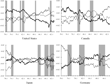
Although our focus in this paper is on the business-cycle properties, we begin our discussion by observing the trend behavior of the key market series and each home series implied by our benchmark parameterization. In each panel of Figure 1, the dashed line shows the behavior of market hours, the lighter solid line shows leisure, and the darker solid line shows home hours for the benchmark parameterization.10
We thank the Foundation for International Business Cycle Research (FIBER) for providing business cycle peak and trough dates.

Market hours (dashed line), leisure (lighter solid line) and home hours (darker solid line). The mean value is subtracted from each series. Shaded regions represent periods of recession.
Figure 1 also shows that leisure rises in each recession recorded in each of the countries. Because market hours are well known to be procyclical, this suggests that in recessions leisure in part replaces market hours. However, changes in leisure tend to be smaller than those in market hours during recessions. This requires that home hours also rise during recessions. Though the cyclical behavior of home hours tends to be less pronounced, as we discuss later, home hours are higher during some recession episodes. Thus, it appears that time out of employment during recessions increases both leisure and home hours.
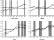
In each panel of Figure 2 the dashed lines show the behavior of market output, the lighter solid line shows market consumption, and the darker solid line shows home consumption for the benchmark parameterization. In the United States and Canada, the decrease in home hours has resulted in a slight decrease in home output. In Japan and Germany, home output has increased. Figure 2 also suggests that home consumption is acyclical or weakly procyclical in the each country. During the 1969–1970, 1980, and 2001 recessions, home output increased in the United States. In the 1973–1975 and 1990–1991 recessions, home consumption fell early in the recession and rose prior to the recession's end. In the 1980–1981 recession, home output fell. In Canada, home hours rose in one recession and were largely unchanged in the other over this period. In the remaining countries, there is again no clear relationship between market and home sector output.

Market output (dashed line), market consumption (lighter solid line), and home consumption under the benchmark parameterization (darker line). The mean value is subtracted from each series. Shaded regions represent periods of recession.
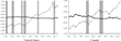
Whereas the behavior of our home hours and leisure series is independent of ρ (see equations (5) and (6)), the behavior of home consumption depends critically on ρ. Figure 3 demonstrates this dependence for the United States and Canada. Each panel shows home consumption at two values of ρ. The darker line is the same series as in Figure 2; that is, ρ=0.5. The lighter solid line is home consumption with ρ=−1.5. When market and home consumption are relative complements (ρ=−1.5), the behavior of the home series is much different for the United States and Canada. In this case, increased market output implies increased production of complementary home output as well.

Home consumption at the benchmark parameterization and ρ = 0.5 (darker solid line) and home consumption withρ = −1.5 (lighter solid line). The mean value is subtracted from each series. Shaded regions represent periods of recession.
Stylized Features of Business-Cycle Dynamics
We now focus more carefully on the business-cycle properties of the major market and home sectors variables in each country. In particular, we study the following features of business-cycle fluctuations: volatility as measured by the percentage standard deviation, persistence as measured by the first-order autocorrelation coefficient, and degree of contemporaneous correlation as measured by the correlation coefficients. Before calculating the moments, we logged and HP filtered all data series. We also provide a detailed comparison of our results with those in the earlier literature that studies the dynamics of the home sector.
Volatility
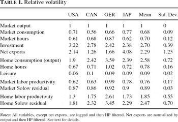
Table 1 displays the volatility of the major market and home variables relative to that of output. Recall that market variables are the observed data series. Our findings regarding these are similar to findings in a number of other studies and the results are similar across countries. Consumption is less volatile than output and investment is on average roughly three times more volatile than output. The relative volatility of net exports is between the relative volatility of investment and output in all countries except Japan, where net exports are the most volatile variable. Market hours are also less volatile than output, and their relative standard deviation is on average close to that of consumption.

Our home series (including leisure) are derived from applying the observables to the mapping implied by the model. Thus, they depend on the observed data, our model, and our choice of parameters. For our benchmark parameters, several interesting regularities emerge. Notice first that the volatility of home hours is slightly larger than that of market hours in each country while leisure is the least volatile series. The standard deviation of leisure is roughly 9% as large as that of output. The relative volatility of home hours is around 80%.
The low variability in leisure is partly explained by equation (5). Given our parameterization, (1−αn)/(1−αm)≈1.19. The average value of
is 0.82 in the United States and is similar in the other countries. Given this, [1−cmt(1−αn)(ymt(1−αm))−1] is close to 0, so that changes in hmt will not result in large changes in leisure. Changes in
will not have a large effect on leisure, for the same reason. Also, these changes are scaled by hmt, which is 0.14 on average, which further diminishes their impact. If we maintain our assumption that market production is more capital intensive than home production, αn is constrained to lie in the internal [0, 0.28]. Over this range, the low standard deviation of leisure is very robust, ranging from 0.0652 to 0.0663 for the United States.
From (6) it is clear that a change in market hours will have a relatively large impact on home hours, giving rise to greater volatility on average (1 + cmtγl[ymt(1−γl)(1−αm)]−1 is clearly not close to 0). In each country, the volatility of home hours is close to that of market hours. Home output, which is equal to home sector output in the model, is more volatile than market output. In particular, the volatility of home output relative to market output ranges from 1.9 in the United States to 3.6 in Germany.
The final rows of Table 1 report volatility in labor productivity (ymt/hmt, ynt/hnt) and the Solow residuals. Solow residual series are calculated employing the production functions of the two sectors.11
Following Backus et al. (1995), we ignore the capital stock series because comprehensive data on quarterly capital stock are not available.

In each country, the volatility of home Solow residuals is greater than the volatility of market Solow residuals and greater than the volatility of output, ranging from 1.3 to 2.61.
Our results pertaining to the U.S. data series are consistent with the qualitative finding of IKS (1997). For example, they find that home consumption is more volatile than market consumption, that market hours fluctuate about as much as home hours, and that leisure is the least volatile series. Moreover, we show that each of these findings holds across all counties in our data suggesting robustness. Quantitatively, our results differ modestly from those of IKS. They find that the relative standard deviations of market hours and home hours are 0.77 and 0.61, compared to 0.61 and 0.67 in our study. Considering that our market hours series comes from a different source and covers a different time period, moderate differences are unsurprising.
IKS also find the relative standard deviations of market and home consumption to be 0.43 and 1.01, compared to 0.71 and 1.90 in our study. This disparity arises in part because our consumption series includes both durable and nondurable consumption components, whereas their series includes only nondurable consumption series. Durable consumption goods are known to be two to three times more volatile than nondurable consumption series (see Baxter (1996)). Their inclusion then increases the volatility of both market and home consumption series.
As mentioned above, studies by BRW, Gomme et al. (GKR, 2001), and Baxter and Jermann (1999) employ closed-economy business-cycle models with a home production sector and calibrate their models to represent the U.S. economy. They make simplifying assumptions about the process of home productivity shocks, feed these shocks to the model to obtain simulated data series, and report the moments of these series. Typically business-cycle researchers compare the moments of their generated series with those of observed data to judge whether the model is successful in replicating observed business cycles. In the case of the home sector, such comparisons are made impossible by data limitations. However, by comparing our moments with theirs we are able at least to gauge the extent to which their models replicate the business-cycle properties of the data series implied by our model.
As in our data, GKR find that home consumption is more volatile than market consumption. The results by BRW and Baxter and Jermann (1999) also suggest that home hours are about as volatile as market hours. In a related study, Canova and Ubide (1998) simulate a two-country business-cycle model augmented with a home production sector. They find that when the model is subjected to only home productivity shocks, the relative volatility of home and market hours is 1.30 and 0.98. When the model is simulated with both market and nonmarket productivity shocks, the relative volatility of home hours is very close to that of market hours. Our results are broadly consistent with these findings.
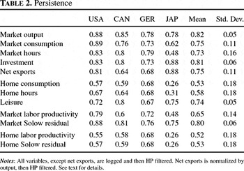
Persistence
Table 2 presents persistence of the series under investigation. The autocorrelation of output is on average 0.82 and it ranges from 0.78 in Germany to 0.88 in the United States. Market consumption, market hours, investment, and the net exports series are quite persistent as well. Home sector variables seem to be less persistent than market variables. For example, the autocorrelation of home consumption is significantly less than that of market consumption in all countries. Similarly, hours employed in the home sector exhibit less inertia than those in the market sector in all countries. However, leisure is highly persistent, with an average autocorrelation coefficient of 0.74.

Comovement
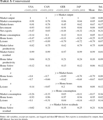
Table 3 documents the contemporaneous correlations of the major market and nonmarket variables with output. As one would expect, consumption, market hours, and investment are procyclical and the net exports series are countercyclical in all countries. Average labor productivity in the market sector is highly correlated with output (0.75) and the fluctuations in the Solow residuals of the market sector closely follow those in sectoral output (near 1).

There is little correlation between home consumption (output) and market output. This correlation ranges from a low of −0.14 in the United States to a high of 0.12 in Germany. Home hours series are on average negatively correlated with market output, ranging from −0.11 in Germany to −0.47 in the United States. The correlation coefficient between leisure and market output does not change much across countries, as leisure is highly countercyclical in all countries, with an average correlation with output of −0.79. Equation (5) suggests that there is a positive correlation between leisure and the ratio of market consumption to output. The ratio of market consumption to output is countercyclical in the data. Thus, leisure is negatively correlated with market output.
We also study lead and lag correlations, which are not presented in a table because of space considerations. Leisure and home hours are both countercyclical at all leads and lags. The (absolute value of the) correlation between leisure and output is larger than that between home hours and output at all leads and lags in all countries. Also, in each country, both home hours and leisure are negatively correlated with market hours. Typically, this correlation is larger (in absolute value) for home consumption. The average contemporaneous correlation between home and market hours is −0.67, and the average contemporaneous correlation between leisure and market hours is −0.79. From these, we conclude that a decrease in market hours is offset by increases in both leisure and home hours. However, as discussed previously, the volatility of leisure is quite small in comparison to the volatility of market hours and home hours. Thus, in large part, an increase in market hours results in a decrease in home hours (and vice versa), as displayed in Figure 1.
The correlation between home hours and leisure is small but differs across countries; it is positive in all countries studied but Canada. The correlation between market consumption and home consumption is negative in all countries (except Germany) and ranges from -0.33 in Canada to only 0.03 in Germany. This implies that increases in market consumption at times coincide with decreases in home consumption and vice versa. Although there is a large positive correlation between home sector output (consumption) and home hours, the correlation between home output and leisure series is negative in all countries except Germany.
Our findings also confirm the qualitative findings of previous simulation studies. For example, IKS find home hours and leisure series are countercyclical in the United States. We also find that home hours are negatively correlated with market output (−0.47) and our leisure series are also negatively correlated with market output (−0.77) in the United States. BRW, GKR, and Canova and Ubide find that home hours are highly countercyclical. Baxter and Jermann find home sector output is positively correlated with market output. However, in each paper the correlation is not always large, ranging from 0.1 to 0.3 and from 0.11 to 0.36. In our findings this ranges from −0.14 in the United States to 0.12 in Germany. Thus while some quantitative differences exist between our results and theirs, this is to be expected given the differences between our approaches and data sets. The finding that the two outputs are not highly correlated largely holds.
Driving processes
A problem facing researchers who work with dynamic business cycle models including a home sector is that they do not have the requisite data to estimate productivity disturbances for this sector. Hence, they use simplifying assumptions regarding the home productivity shock processes. Our approach allows us to evaluate whether these assumptions are reasonable. We assume that productivity disturbances follow a Markov process,

where At=[ln(Amt)ln(Ant)]′ and εt∼N(0, Σ). This specification, which is widely used in the literature, allows us to examine the role of intersectoral spillovers.12
Our major findings are robust to several alternative specifications that take into account the role of intersectoral and intercountry productivity spillovers. The results of these additional estimates are available from the authors upon request.
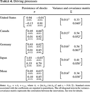
Table 4 documents our findings. There are four major results. First, both market and home productivity shocks are highly persistent. Second, the sectoral feedback coefficient is small in absolute value in all cases. This suggests that it is safe to assume that technological spillovers between market and home sectors are mostly negligible. Third, the standard deviation of the home productivity disturbance is roughly three times larger than that of the market disturbance. Fourth, the contemporaneous correlation between market and home productivity shocks is large and positive in all countries.

BRW assume that both the market and home productivity shocks follow the same process for the United States. GRW and Baxter and Jermann employ the same shock processes as those used by BRW. In particular, the persistence coefficient of each shock is equal to 0.95 and the standard deviation of each disturbance is 0.007. They assume that the correlation between the market and home disturbances is 0.67. Our estimations provide empirical evidence supporting some of these assumptions. We find that the persistence coefficient is around 0.94, which is almost identical to the figure BRW used, for both sectors. The standard deviation of the market disturbance is (0.011) in our study, which is only slightly larger than that of BRW (0.007). However, we also find that the volatility of the home disturbance is roughly three times larger than that of the market disturbance. This conflicts with their assumption of equal volatility of disturbances. The correlation between the two disturbance terms is 0.33 in our study. This is roughly half of the number BRW used. These findings suggest that previous studies consistently underestimate the volatility of home sector productivity shocks while overestimating the correlation between home and market sector productivity disturbances.
Canova and Ubide (1997) assume that the persistence parameter is 0.84 and the standard deviation is 0.007 for both sectors in their open economy business cycle model. They take the correlation between the sectoral disturbances from the BRW study. The intersectoral spillover term is equal to 0.088 in their study. Our estimates indicate that it is reasonable to ignore the sectoral spillover term.
Cross-country correlations
There has been a large and growing body of research that studies international dynamics of business cycles using stochastic dynamic business-cycle models, over the past decade.13
Christodoulakis et al. (1995) find that there are important similarities in the time series properties of labor hours across industrialized economies. Backus et al. (1995) find that the volatility of employment varies from 0.34 to 1.23 in a sample of major industrialized countries. They explain this large disparity with international differences in labor market experience. Kose et al. (2003) provide a brief survey of the literature, which focuses on the similarities of business cycles across countries.
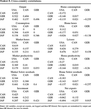
Table 5 presents our findings. In most cases, cross-country output correlations are larger than those of consumption correlations. Stochastic dynamic business-cycle models are not able to generate this empirical regularity, and this gap between the theory and data is called “the quantity anomaly” by Backus et al. (1995). Investment correlations are positive and smaller than those of output in most cases. Fluctuations in market hours tend to be positively correlated across countries, suggesting that the cyclical dynamics in the market sector might have some common features despite the fact there exist major differences in the structural characteristics of labor markets across countries. Net exports have no common pattern, but most correlations are negative. Cross-country correlations of the fluctuations in the market Solow residuals are positive in all cases. Correlations of market productivity are often positive, but they are relatively low, and in most cases lower than those of output.

Overall, home sector variable correlations tend to be lower than their market sector counterparts. Since home output is not a tradable good, this is to be expected. We find that correlations of home consumption (output) are smaller than those of both market output and market consumption. Not surprisingly, correlations of home consumption do not exhibit a clear pattern: four of the six correlations are low and negative, whereas others are low and positive. Cross-country correlations of home hours are smaller than those of market hours in all countries. Leisure series exhibit much higher correlation across countries than home hours do, with all correlation pairs positive. Home productivity correlations do not display much regularity, but most correlations are negative. These correlations are lower than those of market productivity in all cases. Correlations of the Solow residuals of the home sector are low, and they are lower than those of the market sector.
Sensitivity Analysis
We conduct an extensive sensitivity analysis, which is available upon request. Our principal findings prove to be quite robust. Here we emphasize a few items from this analysis. We argued previously that the business-cycle properties of leisure will depend only on (1−αn)/(1−αm), while home hours will depend upon γl/[(1−γl)(1−αm)] and home consumption on both 1/(1−αm)γl/(1−γl) and ρ.
For ease of comparison, we have conducted all of our analysis up to this point with the same parameterization for each country. An alternative approach would be to calibrate each country differently. Zimmermann (1995) reports estimates of αm for each of the countries in our analysis, ranging from 0.37 for the United States to 0.42 for Canada.14
His estimates range from 0.42 for Canada to 0.37 for the United States.
The preference parameter γl has a modest effect on both home hours and home consumption. In each country home output becomes less volatile as we decrease this value. With γl=0.5 home consumption is 1.57 times as volatile as market output on average. Hours in home production become less volatile in each country. The correlation of home output with market output increases and the correlation of home production hours with market output becomes more negative in each country. However, cross-country correlations do not change in a consistent way. As we discuss earlier in the paper, changes in γm do not affect the business cycle moments, but lead to shifts in the level of imputed home consumption series.
In each country, home output becomes less volatile when we decrease ρ to −1.5 but it remains more volatile than market output. On average home output is 2.58 times as volatile as market output with ρ=0.5 and only 1.34 times as volatile with ρ=−1.5. This is an intuitively appealing result because it shows that when the two goods are complements, substitution across them diminishes and the volatility of home output goes down. Persistence of home output also increases slightly on average. Not surprisingly, the comovements of home sector output with market output and market consumption depend on the extent to which these goods are substitutes. With ρ=0.5, the average correlations of home output with market output and market consumption are 0.05 and −0.17. With ρ =−1.5 these are 0.54 and 0.77.
CONCLUSIONS
Recent empirical studies find that the value of household production activities is as much as 50% of aggregate output in several developed countries. Moreover, recent research suggests that studying the dynamics of business cycles in home production is an important component of the modern business cycles research program. However, comparable time-series data on home production activities are not available, because these activities are not observable. Our paper attempts to provide a comprehensive cross-country study of the stylized features of cyclical fluctuations in home production activities using an approach that is complementary to the standard approach.
The results suggest that there are important similarities in the business-cycle properties of the home sector across countries. First, we find that home production is more volatile than market production, that market and home sector hours have similar volatility, and that leisure is much less volatile than other uses of time in all countries. Second, leisure is highly countercyclical in all countries and home hours are countercyclical in all countries. Third, home production variables exhibit less persistence than market variables. Fourth, we find that home production is not highly correlated with market output. Cross-country correlations related to home production tend to be lower than those of market production for both consumption and hours series.
There are some dimensions along which our results differ from previous studies. For example, our findings suggest that previous studies consistently underestimate the volatility of home sector productivity shocks while overestimating the correlation between home and market sector productivity disturbances. Although there are some other minor differences between the features of the home sector business cycles we found and those reported in the previous studies, there are also striking similarities. Because we employ a complementary approach, we take this as evidence of the appropriateness of their assumptions and the robustness of some of their results.
The IKS approach that we employ has similarities to the standard business-cycle approach. Both require calibrated dynamic, stochastic business-cycle models to generate time series for the home sector. In each case, these series are specific to the model and to the choice of parameters. Reservations regarding the choice of parameters can easily be addressed through sensitivity analysis. We conduct such an analysis and find our results to be robust. Reservations regarding the choice of model are not so easily addressed. When one uses “theory for measurement,” the theory used is important. For this reason, we stay close to familiar ground. Our model differs from IKS in a very modest way. IKS, in turn, builds on a frequently employed theoretical framework. Given this, and given that our results are consistent with the standard approach and consistent across countries, we argue that our exercise provides important and robust insights into the cyclical behavior of home production.
There are some interesting questions that can be explored in future research. For example, we do not study the roles of fiscal and monetary policies, which can affect the dynamic interactions between home and market sectors in our model. Moreover, understanding the dynamics of household production is a very useful exercise for developing countries, where home production activities account for a much larger fraction of aggregate output.
A preliminary version of this paper was presented at the Society for Computational Economics Meetings at Yale University in June 2001. We would like to thank an anonymous referee, Ken Beauchemin, Beth Ingram, Robert Kollmann, Kei-Mu Yi, and seminar participants for useful suggestions. Kulaya Tantitemit provided superb research assistance. The views expressed in this paper are those of the author(s) and do not necessarily represent those of the IMF or IMF policy.