2.1 Measurement techniques

The test rig features extensive measurement instrumentation in several measurement planes. The location of the measurement planes is shown in Fig. 3. The reference stagnation pressure ${p_{t,{\rm{E}}0}}$ and the reference stagnation temperature ${T_{t,{\rm{E}}0}}$ are measured in plane E0. The inlet conditions for the numerical simulations are determined in plane E1 with three pressure rakes and three temperature rakes. The dense distribution of the probes near the wall allows the pressure rake in Fig. 4 to measure the incoming boundary layer.

Figure 4.

Boundary layer rake of plane E1 and E2 (Kasper [Reference Kasper11]).

There is an additional boundary layer rake, similar to the one presented in Fig. 4, in plane E2. The rake can be rotated in the circumferential direction. Thus, the outflow pressure field of the swirler and consequently the inflow conditions of the OGVs can be determined.

The main evaluation plane is the ICD outflow plane, labeled with E5. This plane can also be traversed in the circumferential direction and is equipped with another boundary layer rake and a multi-hole probe (MHP). The two probes are positioned 1.5 passages apart to avoid interactions. The MHP is a dual-headed five-hole probe that can be traversed radially in addition to the circumferential direction. The two heads allow fast and efficient measurement of the ICD outflow.

2.2 MHP measurement mesh

The measurement mesh of the MHP is shown in Fig. 5. The mesh of the upper probe is plotted in grey, whereas the mesh of the lower probe is black. The green area represents an ICD passage, and the red line is the position of the upstream strut trailing edge. The upper and lower lines of the mesh are positioned a certain distance away from the walls. This safety distance is important to avoid collisions with the walls and interaction of the probe and the shaft with the boundary layer.

Figure 5.

Measurement mesh of the MHP traverse.

Previous measurements at the TU Berlin rig in Bresemann [Reference Bresemann, Eck, Peitsch, Fritz, Hergt and Rückert17] identified a thin wake that was difficult to capture. Thus, the measurement mesh was refined up to a resolution of 0.5 ${{\rm{\;}}^ \circ }$ behind the strut trailing edge to capture the wake in the DLR measurement campaign. Furthermore, the main task of the campaign was the detailed measurement of the hub region to provide a solid basis for the evaluation of flow control methods at the hub. Therefore, the mesh is also refined in the radial direction towards the hub. The mesh resolution has been validated with numerical data.

2.3 Measurement uncertainties

The measurement uncertainties of stagnation pressures were evaluated according to the Guide to the Expression of Uncertainty in Measurement (GUM) [19]. The measurement chain of the stagnation pressure comprises the ambient and the differential pressure measurement. In addition, the uncertainty of the MHP stagnation pressure ${p_{t,{\rm{E}}5,{\rm{MHP}}}}$ also includes the model uncertainty associated with the multiparameter approximation. The combined uncertainty of the measurement chain was obtained using Gaussian error propagation. The uncertainty associated with the normalisation to the reference pressure ${p_{t,{\rm{E}}0}}$ was also included in the uncertainty propagation. The different uncertainties of the rakes originate from the use of different differential pressure transducers. Plane E1 uses a PSI5 module, whereas the other two planes use a PSI15 module. Furthermore, the MHP pressure measurement is performed using a PSI5 module, which results in lower uncertainty compared to that of the E5 rake. The uncertainties, listed in Table 2, correspond to the expanded uncertainty $U$ , calculated with a coverage factor of (k = 2), representing an approximate confidence level of 95%. According to the MHP calibration, the uncertainty of the circumferential angle $\alpha $ measurement is $ \pm {0.5^ \circ }$ .

Table 1.

Measurement uncertainties for the different measurement techniques

Table 1. Long description

A table titled Measurement uncertainties for the different measurement techniques. The table has two columns and five rows. The columns are labeled Measurement technique and Measurand. The rows are as follows: Row 1: Measurement technique, Measurand; Row 2: E1 rake, p norm, plus or minus 0.00044; Row 3: E2 rake, p norm, plus or minus 0.00058; Row 4: E5 rake, p norm, plus or minus 0.00058; Row 5: E5 MHP, p norm, plus or minus 0.00048; Row 6: E5 MHP, alpha, plus or minus 0.5 degrees.

2.4 Operating point

The investigated operating point is similar to the aerodynamic design point (ADP) presented in Kasper [Reference Kasper11] and Dygutsch [Reference Dygutsch20]. The ADP has an inlet Mach number of $0.32$ and a Reynolds number $3.6$ Mio. The Reynolds number refers to the outer radius of the inlet plane E1. Three percent of the inlet mass flow was extracted as bleed air behind the OGVs. In the following, the measurement point of the ADP is called VRN104.

3.1 Inflow conditions

The inflow conditions of the swirler are measured in plane E1. The time-averaged stagnation pressure profile, determined with the boundary layer rake in Fig. 4, is shown in Fig. 6a. The profile has the typical shape of an undisturbed annular flow with a developed boundary layer at the walls. Outside of the wall regions, the stagnation pressure is almost constant over the radius.

Figure 6.

The inflow conditions of the ICD are measured in plane E1 and E2 with boundary layer rakes.

The coloured band highlights the area between the minimum and maximum measured pressure during the testing time of the measurement point VRN104. The width of the band is a measure of the stability of the operating point. This consideration is important to ensure that the inflow conditions are stable during longer measurement times. Long measurement times occur if a planar traversing of the MHP is conducted, as done for the ADP presented in Fig. 6a. The measurement time for this operating point was approximately 90 minutes. The small deviations of less than 0.2% show that the inlet conditions were highly stable during this long measurement time.

Figure 6a shows the flow field in plane E2 behind the swirler. The plot contains four swirler passages with the corresponding wakes. As already shown by Fritz [Reference Fritz, Dygutsch, Kasper, Hergt, Grund, Flamm, Lejon and Sahota16], the swirler introduces a strong secondary flow field. The flow through the partial gap intensifies the horseshoe vortices and leads to very defined round loss regions. Therefore, the OGVs experience a non-uniform inflow. The numerical studies of Fritz [Reference Fritz, Dygutsch, Kasper, Hergt, Grund, Flamm, Lejon and Sahota16] concluded that the interaction of the secondary flow system of the swirler with the OGVs causes separations on the OGVs. The resulting losses are convected towards the hub by the radial pressure gradient in the first bend. This effect destabilises the hub boundary layer and could cause an earlier onset of the separations.

3.2 Outflow conditions

The measurement plane E5 is instrumented with an MHP and a boundary layer rake to determine the ICD outflow conditions. The measurement data from this plane can be used to draw conclusions about the flow conditions and, in particular, the separations in the ICD. Figure 7 presents the normalised stagnation pressure field measured with the MHP. In the radial direction, the MHP cannot measure the regions close to the wall because of a required safety distance.

Figure 7.

Normalised stagnation pressure field at the ICD outlet measured with the MHP.

The pressure field in Fig. 7 shows the typical structure of a highly aggressive ICD. The flow field is asymmetric, and the wake is bended. There is also a loss region on the right side of the wake $\unicode{x2460}$ close to the hub. This loss region is typically caused by a corner separation at the right hub corner. Another distinct loss region $\unicode{x2461}$ is located on the left side of the wake between −30 ${{\rm{\;}}^ \circ }$ and −25 ${{\rm{\;}}^ \circ }$ . These losses are generated by a separation in the ICD passage close to the left side of the strut.

The shroud region has a very high loss level throughout the circumference, except the region from −30 $^ \circ $ to −25 $^ \circ $ $\unicode{x2462}$ . In this region, a strong vortex should exist. This vortex represents the left leg of the upper strut horseshoe vortex. But this region is too disturbed for the MHP. The flow is misaligned, and the probe cannot capture the strong horseshoe vortex in this area.

The boundary layer rake in plane E5 is also traversable in the circumferential direction. Thus, a stagnation pressure field similar to the one measured with the MHP in Fig. 7 can be derived from the rake data. The normalised stagnation pressure field of the boundary layer rake is shown in Fig. 8. The flow structure is identical to the field measured with the MHP in Fig. 7. The wake is less resolved in the circumferential direction because of the difference between both measurement devices of 1.5 passages. Therefore, the wake is now located in coarse areas of the measurement mesh (compare Fig. 5). Furthermore, the boundary layer rake has a coarser resolution of the mean flow.

Figure 8.

Normalised stagnation pressure field at the ICD outlet measured with the boundary layer rake.

However, further information about the flow conditions close to the walls is provided by the rake. At the shroud, the left leg of the horseshoe vortex $\unicode{x2460}$ is clearly visible. This loss region cannot be captured by the MHP because the secondary flow is so strong that the probe is misaligned with the flow. Furthermore, the loss region $\unicode{x2461}$ at the hub on the left side of the wake has a significantly larger circumferential expansion than measured with the MHP. The loss region ranges from −18 ${{\rm{\;}}^ \circ }$ until the wake and covers almost half a passage. The MHP cannot measure in this region because of the safety distance to the wall. The presence of this loss region is a clear indication of a separation in the right part of the passage (aft-lookingforward (ALF)).

Figure 9.

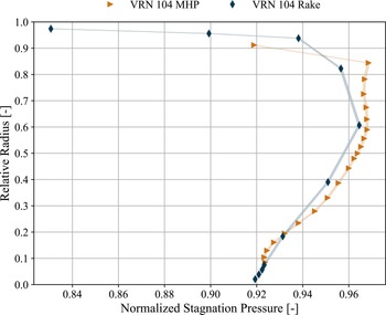
Comparison of the normalised stagnation pressure profiles in plane E5 measured with the boundary layer rake and the MHP.

Finally, the pressure fields of the rake and the MHP are area-averaged over the circumference. Figure 9 compares the resulting stagnation pressure profiles. The shaded uncertainty band represents the expanded uncertainty with a coverage factor of k = 2 according to Table 1. The profiles are in very good agreement, especially in the lower half of the channel. The MHP profile is more detailed because of the larger number of radial measurement positions. Especially in the region of 10–20% channel height, the profile provides more information about the shape of the stagnation pressure distribution. On the other side, the rake data are a perfect extension of the MHP profile below 10% channel height. With increasing radius, the differences increase. A cause is the averaging method. The averaging is conducted with cell-averaged values. Thus, the average pressure is an average of values from two different radial heights. This could lead to differences in regions of large gradients and coarse resolution. The pressure profiles are further influenced by the different resolution of the wake. The comparison highlights the advantages of both measurement techniques. The rake provides detailed information about the regions close to the walls where the MHP cannot operate. However, the radial resolution of the MHP can be easily adapted to resolve regions of interest. Therefore, both methods are highly complementary.

The huge advantage of the MHP measurement is the calculation of the flow angles. The planar distribution of the circumferential flow angle $\alpha $ is shown in Fig. 10. The wake of the strut is again clearly visible $\unicode{x2460}$ as a shear layer. On the left side of the wake, the flow angle is positive, on the right side negative. At the hub, there is a huge gradient between positive and negative flow angles $\unicode{x2461}$ at around −27 ${{\rm{\;}}^ \circ }$ . This location coincides with the high-loss region left from the wake in Fig. 7. The sharp gradient between negative and positive angles is an indication of a strong streamwise vortex. The vortex core aligns with the centre of the losses $\unicode{x2461}$ in Fig. 7.

Figure 10.

Circumferential angle $\alpha $ field in plane E5. An angle $\alpha = 0$ is equivalent to a purely axial flow.

A large region of high negative flow angles occurs at the shroud and the hub. Also, there is a region of high positive flow angles $\unicode{x2462}$ on the left side of the wake. Thus, the flow field shows on a constant radius large deviations and gradients of the circumferential flow angle $\alpha $ . The highly inhomogeneous flow field could influence the performance of the downstream HPC.

4.1 Boundary conditions

The inlet conditions for stagnation pressure and stagnation temperature are derived from the measurements. Pressure and temperature rakes are installed in inlet plane E1. Kasper [Reference Kasper, Dygutsch, Grund, Beversdorff, Hakansson, Nicke and Lejon10] has already shown that the inflow conditions are uniform. Therefore, the data are time-averaged and prescribed as radial profiles. Figure 6a shows the stagnation pressure profile used as a boundary condition. Furthermore, a purely axial inflow is assumed. The turbulence intensity and turbulence length scale were taken from previous hot-wire measurements for the same operating point, conducted by Kasper [Reference Kasper, Dygutsch, Grund, Beversdorff, Hakansson, Nicke and Lejon10].

Mass flow measurements are applied in the ICD rig for inlet and bleed mass flow rate via orifice flow meter sections. The difference between both measurement is time-averaged and prescribed as an outlet boundary condition. Furthermore, a bleed mass flow rate of 3% is extracted behind the OGVs.

4.2 ICD outlet pressure distribution

The results of the numerical simulation with different turbulence models are presented in Fig. 11. The plots show the normalised stagnation pressure field in plane E5. The results are interpolated on the experimental mesh to achieve comparability with the experimental fields in Figs 7 and 8. Thus, the regions close to the walls are also excluded. The position of the wake in the numerical plots is identical to the position in the MHP measurements in Fig. 7.

The structure of the SST pressure field in Fig. 11a shows significant deviations from the experimental data (Fig. 7). The shape of the wake is fundamentally different. The wake is wider, and loss regions of elliptical shape occur at around 40% channel height on the left side $\unicode{x2460}$ and at around 50–60% on the right $\unicode{x2461}$ of the strut. These losses are caused by the horseshoe vortex on the hub of the strut. Thus, the lower horseshoe vortex separates from the hub on both sides. This behaviour is not observed in the experiments. Furthermore, the upper part of the wake $\unicode{x2462}$ differs from the experiments and the other simulations. The loss level is higher, and the wake is wider above 80% channel height.

The pressure field of Hellsten (Fig. 11b) and RSM (Fig. 11c) are similar. Both simulations show a flow structure that is similar to the experiments. For both simulations, the wake is bent, and a round loss region occurs on the left side of the wake $\unicode{x2460}$ . The loss region is predicted closer to the strut trailing edge than measured in the experiments. The centre of this loss region is located between −25 ${{\rm{\;}}^ \circ }$ and −20 ${{\rm{\;}}^ \circ }$ in both simulations and not between −30 ${{\rm{\;}}^ \circ }$ and −25 ${{\rm{\;}}^ \circ }$ observed in the experimental data. Thus, the numerical simulations show a discrepancy of about 5 $^ \circ $ in the circumferential position of this loss region. Furthermore, the loss region is larger and has higher losses for the RSM simulation (Fig. 11c). Among all turbulence models, the Hellsten model agrees best with the experimental data in Fig. 7.

However, the loss region around −5 ${{\rm{\;}}^ \circ }$ $\unicode{x2461}$ cannot be observed in the experimental data in Fig. 7. The loss region occurs in both the RSM and Hellsten simulations. The region is more defined in the Hellsten simulation. In contrast, this region has a very low loss level in the experiments. Thus, the numerical simulation predicts another loss mechanism that cannot be observed in the experimental data.

Figure 11.

Comparison of the stagnation pressure field in plane E5, calculated with different turbulence models.

4.3 Separation topology

The numerical simulations have the huge advantage that a three-dimensional volume can be investigated. Every point in the numerical domain is accessible. Besides the uncertainties in the turbulence modeling, the simulations are a valuable tool for visualising flow structures. The experiment at the DLR rig cannot visualise the topology of the separations in the ICD. Only the effects of the separations can be observed in the stagnation pressure field at the outlet plane E5 as regions of high loss levels.

Figure 12 shows two different analyses of the flow field in the Hellsten simulation. The view is against the flow direction (ALF). The simulation using the Hellsten turbulence model was selected, as the previous section showed that it provides the best agreement with the experimental data. Figure 12a visualises the separations in the ICD by iso-surface with the criterion ${v_x} \lt 0$ . The hub boundary layer experiences two distinct separations. A hub corner separation $\unicode{x2460}$ occurs at the right side of the strut (ALF). Another separation bubble $\unicode{x2461}$ forms in the passage close to the left side of the strut.

Figure 12.

Flow field of the simulation with the Hellsten turbulence model (ALF). Green surfaces visualise negative axial velocities ${v_x} \lt 0$ and thus, flow separations. The streamlines indicate the origin of the losses in Fig. 11.

Figure 12. Long description

A diagram of the flow field simulation with the Hellsten turbulence model. Panel A: Separation topology. This panel shows a three-dimensional view of flow separations visualized by green surfaces indicating negative axial velocities. The separations are labeled as 1 and 2. Panel B: Origin of the loss regions. This panel shows streamlines indicating the origin of losses, with regions labeled as 1, 2, and 3. The streamlines are color-coded to represent normalized stagnation pressure, with a legend indicating values ranging from 0.85 to 0.92. The flow field is visualized within a duct-like structure, showing the interaction between the flow and the duct walls.

The numerical simulations enable the losses to be linked to distinct flow mechanisms. Thus, Fig. 12b investigates the origin of the loss regions in plane E5. The normalised planar stagnation pressure distribution in plane E5 is shown in the figure. The regions with ${p_{t,norm}} \gt 0.92$ are transparent to provide a better view of the flow field. Also, the incoming losses are visualised in the same manner. The streamlines illustrate the origin of the losses. Blue streamlines $\unicode{x2460}$ are linked to the loss region on the left side of the wake. The losses are associated with the passage separation. The origin of the losses on the right side of the wake is highlighted with red streamlines $\unicode{x2461}$ . These losses are generated by the hub corner separation.

The previous paragraph concludes that the numerical simulations (Hellsten and RSM) contain another loss mechanism that is responsible for the loss region at −5 ${{\rm{\;}}^ \circ }$ in Fig. 11b and c. Yellow streamlines $\unicode{x2462}$ visualise the origin of these losses. The losses are not associated with any separation in the ICD but rather with a specific OGV wake. The loss mechanisms of the upstream components have already been described in Section 3.1 and Fritz [Reference Fritz, Dygutsch, Kasper, Hergt, Grund, Flamm, Lejon and Sahota16]. The interaction of the swirler secondary flow system with the OGVs causes larger flow separations on every second vane. Furthermore, the upstream effect of the strut enhances the separations on the OGVs ahead of it. These effects generate the incoming loss region that later forms the loss region $\unicode{x2461}$ in Fig. 11b and c. In summary, the numerical simulations struggle to predict either the loss generation upstream of the strut or the development of the incoming losses in the ICD.

4.4 Radial stagnation pressure profile

The analysis of the numerical stagnation pressure field in Fig. 11 identified differences in the flow structure. However, a quantitative comparison requires the evaluation of the radial profiles. Therefore, the numerical results were circumferentially area-averaged. The comparison of the resulting stagnation pressure profiles is shown in Fig. 13. All numerical methods overestimate the losses in the ICD. Especially the SST turbulence model predicts higher losses between 70% and 85% channel height. This region is not significantly affected by secondary flow phenomena. The reason for the higher losses is the wider wake in Fig. 11a. The Hellsten and RSM turbulence models are able to reproduce this region in very good agreement with the experimental data. Notably, the predicted losses in the end wall regions for the SST model show good agreement with the experimental data.

Figure 13.

Comparison of the numerical and experimental radial stagnation pressure profiles in plane E5.

The pressure profiles of Hellsten and RSM show the same characteristics. Above 70% channel height, the profiles are very close to the experimental data. The shape of the Hellsten profile is similar to the experimental data below 70% channel height. However, the simulations overpredict the losses in the lower part of the channel. The same behaviour is observed in Fig. 11b and c, where the loss level in the lower part of the wake is higher than in the experiments in Fig. 7. Nevertheless, the shape of the Hellsten pressure profile is similar to the experimental data. This again highlights that the simulations struggle to accurately reproduce the losses in the ICD.

4.5 ICD pressure losses

Finally, the stagnation pressure loss $\omega $ is calculated according to Equation (1) via area-averaging the normalised stagnation pressure field for the experiment and the simulations.

(1) \begin{align}\omega = 1 - \frac{{{p_{t,{\rm{E}}5}}}}{{{p_{t,{\rm{E}}0}}}} \end{align}

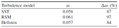
Table 2 lists the stagnation pressure losses for the different turbulence models and their difference to the measured value in percent. The stagnation pressure loss measured with the MHP is 0.031. The stagnation pressure losses in Table 2 underline the finding of the previous section. The numerical simulation is significantly overestimating the losses in the ICD. The RSM turbulence model predicts losses that are almost twice as high as the measured value. Although the other turbulence models yield lower losses, the deviation from the measured value remains very high at over 80%.

Table 2.

Comparison of the numerical stagnation pressure losses with the measured loss

Table 2. Long description

A table comparing turbulence models and their corresponding values. The table has three rows and three columns. The columns are labeled ‘Turbulence model’, ‘ω’, and ‘Δω (%)’. The rows are labeled with different turbulence models: SST, RSM, and Hellsten. The values in the table are as follows: Row 1: Turbulence model, SST; ω, 0.058; Δω (%), 87. Row 2: Turbulence model, RSM; ω, 0.061; Δω (%), 97. Row 3: Turbulence model, Hellsten; ω, 0.057; Δω (%), 84.

5.1 Outlet flow field

Figure 15 shows the Mach number field in the ICD outlet plane E5 of the TU Berlin ICD, measured with an MHP. The Mach number field is used to demonstrate that both rigs operate at comparable Mach number levels and to illustrate the distribution of dynamic pressure within the flow field. The trailing edge of the ICD is at the ${0^ \circ }$ position (dashed line). Of particular note are the extensive regions of low Mach numbers observed at the shroud $\unicode{x2460}$ $\unicode{x2462}$ . These regions are related to a very strong horseshoe vortex. Furthermore, this counter-rotating vortex pair generates a large separation accompanied by high losses at the shroud, as shown in Bresemann [Reference Bresemann, Eck, Peitsch, Fritz, Hergt and Rückert17] and Fritz [Reference Fritz, Koppers, Hergt, Bresemann, Eck, Peitsch, Möller and Rückert27]. Another region of low Mach number $\unicode{x2461}$ is observed on the right side of the trailing edge in the lower part of the channel. This region results from a strong hub-corner separation. An additional small region of low Mach numbers $\unicode{x2463}$ appears at the hub at around $ - {10^ \circ }$ . The cause of this region is a small passage separation.

Figure 15.

Outlet Mach field of the scaled TU Berlin ICD.

Figure 16.

Outlet Mach field of the full-size DLR ICD in plane E5.

The Mach number field of the DLR ICD rig is shown in Fig. 16. The trailing edge of the ICD is at around $ - {22^ \circ }$ (dashed line). A low Mach number region $\unicode{x2460}$ appears at the hub between $ - {30^ \circ }$ and $ - {25^ \circ }$ . This region originates from the passage separation. Also, the right hub corner has a region of reduced Mach number $\unicode{x2461}$ . The hub-corner separation causes this loss region. However, the region is reduced compared to the TU Berlin rig. In summary, the passage separation is stronger for the DLR ICD rig while the hub-corner separation is smaller.

In both rigs, the left side of the upper horseshoe $\unicode{x2462}$ is pronounced. Furthermore, the horseshoe vortex is significantly weaker in the DLR ICD rig, and the shroud separation is considerably smaller. This finding supports the assumption of Fritz [Reference Fritz, Koppers, Hergt, Bresemann, Eck, Peitsch, Möller and Rückert27] that the presence of an HPC-IGV row would significantly reduce the size of the shroud separation of the TU Berlin rig. Thus, the shroud separation of the TU Berlin is not representative for a highly aggressive ICD in a jet engine environment.

5.2 Radial stagnation pressure profile

Finally, both rigs can be compared by the stagnation pressure profiles at the ICD outlet. Figure 17 shows the measured radial stagnation pressure distribution. The uncertainty of the TU Berlin pressure measurement is 0.05%. Furthermore, the combined uncertainty of the normalisation is obtained using Gaussian error propagation. The shaded uncertainty band again represents the expanded uncertainty for both rigs. The setup of the TU Berlin does not include a swirler row. In order to ensure a fair comparison between both rigs, the stagnation pressure of the DLR ICD is normalised by the average stagnation pressure of plane E2 ${p_{t,{\rm{E}}2,0{\rm{D}}}}$ . Thus, the control volume includes the OGVs and the ICD.

Figure 17.

Comparison of the radial outlet stagnation pressure distribution of the twins.

The effect of the shroud horseshoe vortex in the TU Berlin rig is also reflected in the stagnation pressure profile. The losses are significantly higher in this region. The radial extent of the shroud loss region is also larger. In the TU Berlin rig, the loss region extends down to 60% channel height, whereas in the DLR rig, the region only reaches down to 85%. Beneath the shroud loss region, there is a maximum in the stagnation pressure profile. For the DLR rig, this maximum is a region of almost constant pressure from 60% to 85% channel height. The maximum for the TU Berlin rig is round with a peak around 60%. Below 50% channel height, the shape of the profiles is similar. The losses increase monotonically towards the hub until 10%. Especially, the local minimum at this height exists in both profiles. Thus, the loss generation of the TU Berlin below 50% channel height is representative of the full-scale DLR ICD rig. Consequently, the TU Berlin is suitable for the investigation of flow control methods on the ICD hub. The transferability of the results to the DLR rig is ensured by the similarity of the flow structures.

It is noteworthy that the losses of the DLR ICD are higher than those of the TU Berlin ICD except in the shroud region. Especially below 50% channel height, the pressure profiles seem to be shifted by a constant value. The reason for this is the OGV row. The OGVs of the DLR rig are highly loaded due to the preswirl introduced by the swirler. The TU Berlin rig operates without preswirl and, thus, the OGVs are significantly less loaded. Furthermore, the DLR ICD features double the number of OGVs. The larger wetted surface increases the friction losses in this row. In addition, the secondary flow system of the swirler induces alternating separation on the OGV suction side. This effect has already been investigated in Fritz [Reference Fritz, Dygutsch, Kasper, Hergt, Grund, Flamm, Lejon and Sahota16] for the DLR ICD rig and visualised in Fig. 12b. These separations cause further losses. CFD simulations conducted with the Hellsten turbulence model conclude that the losses of the DLR OGV are more than 15 times higher than the TU Berlin OGV losses. Thus, the differences in the OGV row mainly cause the higher loss level of the DLR ICD outside the shroud region.