

1. Introduction
An understanding of the hydrodynamics of a quasi-two-dimensional fluid interface coupled to a bulk three-dimensional (3-D) subphase is crucial to modelling the dynamics of a wide variety of biological systems such as lipid membranes (Stone & McConnell Reference Stone and McConnell1995), bacterial biofilms (Petroff, Wu & Libchaber Reference Petroff, Wu and Libchaber2015) and algae colonies (Drescher et al. Reference Drescher, Leptos, Tuval, Ishikawa, Pedley and Goldstein2009). One notable theoretical and experimental study of such a system was conducted by Alexander et al. (Reference Alexander, Bernoff, Mann, Mann and Zou2006), who examined the tension-driven closing of a cavity punctured in a poly(dimethylsiloxane) (PDMS) monolayer situated on a flat water–air interface. The authors derived an analytical solution for the axisymmetric fluid motion, predicting that the area of the cavity decreases at a fixed rate that depends only on the ratio of monolayer line tension to subphase viscosity; by fitting experimental data in a linear regime of the area versus time plot, they obtained an estimate for the line tension. The same authors later reapplied this model along with improved experimental methods to obtain a more accurate value for the monolayer line tension, which they reported to be  $0.69\pm 0.02$ pN in Zou et al. (Reference Zou, Bernoff, Mann, Alexander and Mann2010).
The reduction of this problem to the fitting of a single parameter hinges on a crucial assumption: the monolayer viscosity is vanishingly small. Although there is experimental evidence supporting the claim that the film dynamics is dominated by subphase viscosity rather than monolayer viscosity (Jarvis Reference Jarvis1966; Mann et al. Reference Mann, Hénon, Langevin, Meunier and Léger1995), and although there are strongly linear regimes in the experimental area versus time data in both Alexander et al. (Reference Alexander, Bernoff, Mann, Mann and Zou2006) and Zou et al. (Reference Zou, Bernoff, Mann, Alexander and Mann2010), the data as a whole are visibly nonlinear, especially at later times when the hole size is small. This indicates that the authors’ assumptions may not hold as well as they initially believed and that other effects may be playing a role in the closure process. One potential explanation for the nonlinearity is that monolayer viscosity decelerates the interface when the hole becomes small.
Here we revisit the theoretical model proposed by Alexander et al. (Reference Alexander, Bernoff, Mann, Mann and Zou2006) and amend it by considering the effects of a regularising monolayer viscosity. This simple change preserves much of the structure of the problem but introduces some notable differences. We find that although the bulk equations are unchanged in the axisymmetric case, the boundary conditions can depend strongly on this monolayer viscosity, especially in regimes where the cavity radius is small relative to the Saffman–Delbrück length, that is, the ratio of the two-dimensional (2-D) monolayer and 3-D bulk viscosities. In this regime, the predicted dependence of cavity area on time becomes noticeably nonlinear, which affects the fitting of experimental data and consequently suggests that these previous studies have underestimated the edge tension by roughly one order of magnitude.
We begin with an overview of the physical system and experiments of Alexander et al. (Reference Alexander, Bernoff, Mann, Mann and Zou2006) and introduce our idealised model and its limitations in § 2. In § 3, we formulate the model mathematically and demonstrate its solution in the annular geometry, focusing on the case where the outer radius is much larger than the inner radius and analytical solutions are available. The results of Alexander et al. (Reference Alexander, Bernoff, Mann, Mann and Zou2006) are discussed as a limiting case of our model. We then proceed to compare the results of both models against their experiments in § 4 and conclude in § 5.
2. Physical system and model
The experimental system of Alexander et al. (Reference Alexander, Bernoff, Mann, Mann and Zou2006) consisted of a subnanometer thin PDMS layer resting on top of an aqueous substrate in a classic Langmuir trough. PDMS is well-known in the polymer community for its relatively weak intermolecular forces, leading to a low surface tension and very low surface viscosity (Jarvis Reference Jarvis1966). Depending on the density, the film may separate into coexisting gas and liquid phases; due to the line tension, these liquid domains tend to be stable and round in shape. The experiments in Alexander et al. (Reference Alexander, Bernoff, Mann, Mann and Zou2006) involved using a platinum wire of diameter 0.13 mm to quickly puncture liquid domains of characteristic size of approximately 0.01 mm2. The resulting hole of polymer gas was observed to close up completely over the course of roughly 20 s.
The fluid dynamical model of Alexander et al. (Reference Alexander, Bernoff, Mann, Mann and Zou2006) treats the liquid domain and subphase as a coupled system of fluids governed by the Stokes equations and driven by line tension. In particular, the liquid polymer domain is taken to be a 2-D incompressible surface inviscid phase, so that its bulk dynamics are governed solely by a pressure gradient. Our model relaxes this assumption and considers the liquid phase to be a viscous Newtonian fluid. Both models are idealised and so neglect a diversity of physical effects that have been observed to play a role in the dynamics of polymer Langmuir films. Some of these effects include the following.
(i) Cavity polymer concentration and accretion on/evaporation of the edge of the liquid domain. For polymer Langmuir films, the cavity is not a true vacuum but may contain a sparse amount of molecules in a gas phase. Assuming no exchange of molecules between the gas and liquid phases, the relaxation of the interface implies that the polymer density inside the cavity increases over time. Thus, as the cavity shrinks, there is potentially a gaseous pressure contribution that slows the interface. In the experiments of Alexander et al. (Reference Alexander, Bernoff, Mann, Mann and Zou2006), the polymer density inside the cavity was found to be immeasurably small throughout the duration of the experiments. We hence likewise only concern ourselves with the dilute gas limit in which the cavity surface pressure vanishes. For non-dilute gases, our model can be modified in a straightforward manner by assuming an equation of state for the cavity that relates pressure and concentration of molecules. Mass transfer between phases may similarly be accounted for with a generalisation of our model.
(ii) Electrostatic effects. The intermolecular forces between polymer molecules give rise to a line tension between the liquid and gas phases, which Alexander et al. (Reference Alexander, Bernoff, Mann, Mann and Zou2006) identify as the primary driver of motion. The two phases in general have different electrostatic potentials, and this may cause some distortion of the domain. For the domain sizes considered by Alexander et al. (Reference Alexander, Bernoff, Mann, Mann and Zou2006), the effect of long-range electrostatic interactions is primarily to renormalise the line tension. The leading-order correction is logarithmic, suggesting that the line tension may be taken to be constant over a wide range of length scales (de Koker & McConnell Reference de Koker and McConnell1993), including those in which the experiments took place. We will therefore also assume the line tension is a constant independent of domain size.
(iii) Polymer elasticity. A number of studies such as Khattari et al. (Reference Khattari, Hatta, Heinig, Steffen, Fischer and Bruinsma2002) model Langmuir films as viscoelastic fluids. In general, such materials are, to leading order, characterised not only by shear and dilitational viscosities but also by shear and dilitational elasticities. For the polymer material in question with area
 $A$ and 2-D tension $\varPi$, the Gibbs elasticity of the liquid phase $K_{G} = \partial \varPi /\partial (\log A)$ has been measured to be approximately 40 mN m$^{-1}$ (Mann & Langevin Reference Mann and Langevin1991), several orders of magnitude larger than the scale defined by the line tension divided by the characteristic length of the domain. The monolayer is thus taken to be effectively incompressible in our analysis so that the dilitational viscosity and elasticity both vanish. Here, in keeping with the study of Alexander et al. (Reference Alexander, Bernoff, Mann, Mann and Zou2006), we elect to focus on the simplest case where the motion is driven entirely by incompressible fluid mechanics and not elasticity. The key difference of our approach from that of Alexander et al. (Reference Alexander, Bernoff, Mann, Mann and Zou2006) is that we do not assume the monolayer shear viscosity vanishes. The cavity itself is notably extremely compressible, with a Gibbs elasticity too small to measure.


We recognise that any subset of the non-fluid dynamical effects listed above could be of importance in determining the cavity dynamics. Nonetheless, we find that the simplest possible modification of the Alexander et al. (Reference Alexander, Bernoff, Mann, Mann and Zou2006) model, namely the inclusion of a monolayer viscosity without accounting for the above processes, leads to a mathematical analysis that, while technical, visibly sharpens the fits of the experimental data.
3. Mathematical formulation
3.1. Geometry and equations of motion
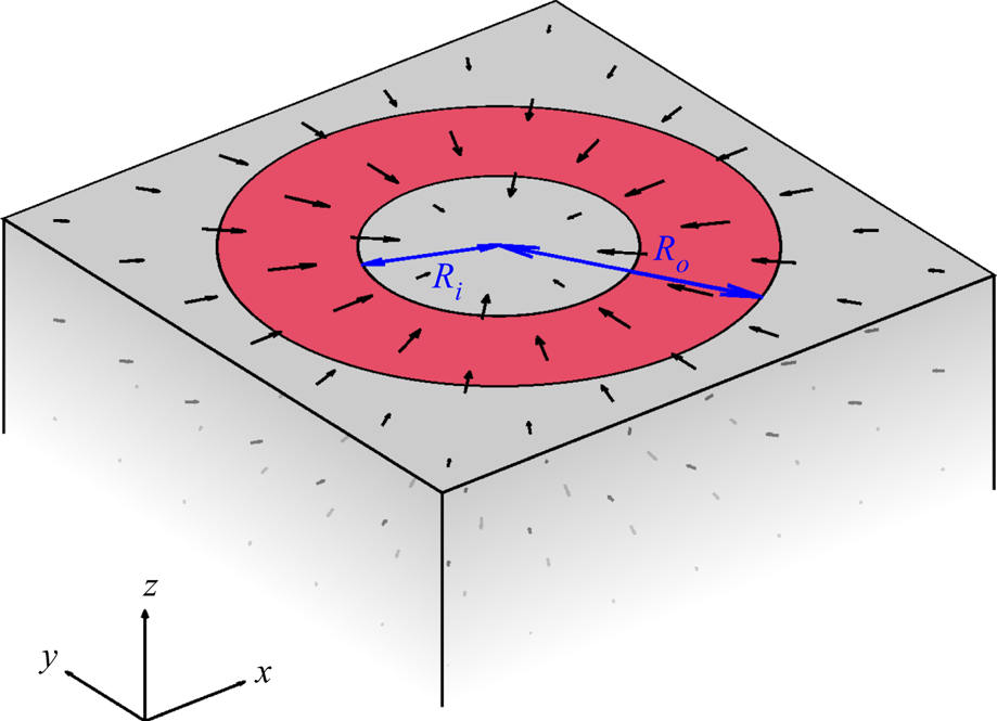
Consider a molecularly thin (so essentially 2-D) fluid monolayer situated on a 3-D half-space of Stokes fluid (figure 1). Let the subphase have flow field  $\boldsymbol {u}$, pressure
 $p$ and viscosity
 $\mu$. We assume the subphase satisfies the incompressible Stokes equations
 \begin{equation} -\!\boldsymbol{\nabla}_{3D} p + \mu \boldsymbol{\nabla}_{3D}^{2} \boldsymbol{u} = 0\quad\text{and}\quad \boldsymbol{\nabla}_{3D}\boldsymbol{\cdot} \boldsymbol{u} = 0,\end{equation}
where  $\boldsymbol {\nabla }_{3D} = (\partial /\partial x,\partial /\partial y, \partial /\partial z)$ is the 3-D gradient operator.
Schematic of an annular Langmuir monolayer domain  $\mathcal {D}$, with inner radius
 $R_i$ and outer radius
 $R_o$, situated on the upper surface of a Stokesian sublayer of infinite depth, whose motion generates a shear stress on the monolayer. Where
 $0< r< R_i$ or
 $r>R_o$, the surface is stress-free. The corresponding instantaneous velocity fields both in the subphase
 $\boldsymbol {u}$ and at the surface
 $\boldsymbol {U} = \boldsymbol {u}(z=0)$ are shown; vectors are coloured by depth.

Let  $\mathcal {D}$ be a subset of the
 $z=0$ plane that a domain of the liquid phase occupies. For our analysis, we take the monolayer liquid phase to be a Newtonian fluid with velocity
 $\boldsymbol {U}$, 2-D pressure
 $P$ and shear viscosity
 $\eta$. (A more detailed treatment could consider other effects.) Continuity of the flow field implies
 $\boldsymbol {U} = \boldsymbol {u}(z=0)$. The stress tensor of such a fluid is
 \begin{equation} \boldsymbol{\sigma} ={-}P {\boldsymbol{\mathsf{I}}} + \eta (\boldsymbol{\nabla}\boldsymbol{U} + \boldsymbol{\nabla} \boldsymbol{U}^{T}),\quad \boldsymbol{x}\in\mathcal{D}, \end{equation}
where  $\boldsymbol{\nabla}$ is the 2-D gradient operator in the xy-plane. The transverse motion of the subphase generates a surface shear stress on the monolayer so that
 \begin{equation} \boldsymbol{\nabla}\boldsymbol{\cdot} \boldsymbol{\sigma} ={-}\boldsymbol{\nabla} P + \eta {\rm \Delta} \boldsymbol{U} = \left. \mu \frac{\partial \boldsymbol{u}}{\partial z}\right|_{z=0} \quad\text{and}\quad \boldsymbol{\nabla}\boldsymbol{\cdot} \boldsymbol{U} = 0,\quad \boldsymbol{x}\in \mathcal{D}, \end{equation}
where  $\Delta$ is the 2-D Laplacian in the xy-plane. Outside of the domain
 $\mathcal {D}$ (i.e. in its complement
 $\mathcal {D}^{C}$), we assume the interface is stress-free:
 \begin{equation} 0 = \left. \mu \frac{\partial \boldsymbol{u}}{\partial z}\right|_{z=0},\quad \boldsymbol{x}\in \mathcal{D}^{C}. \end{equation}
The surface is assumed to be planar for all times, and the flow field of the interface  $\boldsymbol {U}$ is assumed to have no
 $z$-component. Lastly, we consider the one-dimensional interface
 $\partial \mathcal {D}$, where balancing stresses demands that
 \begin{equation} \boldsymbol{\sigma} \boldsymbol{\cdot} \hat{\boldsymbol{n}} |_{\partial\mathcal{D}}= \gamma \kappa \hat{\boldsymbol{n}}|_{\partial\mathcal{D}},\end{equation}
with  $\hat {\boldsymbol {n}}$ is the local normal vector to the curve
 $\partial \mathcal {D}$ and
 $\kappa$ is the local curvature.
Following Alexander et al. (Reference Alexander, Bernoff, Mann, Mann and Zou2006), we restrict ourselves to the axisymmetric case where the domain of the monolayer is an annulus centered at the origin in the  $z=0$ plane. In cylindrical coordinates
 $(r,\theta,z)$, the monolayer domain
 $\mathcal {D} = \{(r,\theta,0): 0< R_i< r < R_o\}$, where
 $R_o$ is allowed to be positive infinity. We further assume there are no azimuthal stresses, so that the azimuthal component of
 $\boldsymbol {U}$ vanishes. In this setting, (3.1a,b) simplifies to
 $$\begin{gather} -\frac{\partial p}{\partial r} + \mu \left(\mathcal{L}_1[u] + \frac{\partial^{2} u}{\partial z^{2}}\right)=0, \end{gather}$$
 $$\begin{gather}-\frac{\partial p}{\partial z} + \mu \left(\mathcal{L}_0[w] + \frac{\partial^{2} w}{\partial z^{2}}\right)=0, \end{gather}$$
 $$\begin{gather}\frac{1}{r}\frac{\partial (ru)}{\partial r} + \frac{\partial w}{\partial z}=0, \end{gather}$$
where  $u$ and
 $w$ are the radial and
 $z$-components of
 $\boldsymbol {u}$, respectively, and
 \begin{equation} \mathcal{L}_\nu = \frac{\partial^{2}}{\partial r^{2}} + \frac{1}{r}\frac{\partial}{\partial r} -\frac{\nu^{2}}{r^{2}}. \end{equation}
At the surface, we have
 \begin{equation} \left(-\frac{\mathrm{d}P}{\mathrm{d} r} + \eta \mathcal{L}_1[U]\right)\chi(R_i< r< R_o) = \left. \mu \frac{\partial u}{\partial z}\right|_{z=0},\end{equation}
where  $U(r) = u(r,z=0)$ and
 $\chi$ is a characteristic function. Additionally, the incompressibility condition for the monolayer takes the form
 \begin{equation} \frac{1}{r}\frac{\partial (rU)}{\partial r} = 0,\quad R_i< r< R_o, \end{equation}
from which we conclude
 \begin{equation} U(r) = \frac{F}{r},\quad R_i< r< R_o,\end{equation}
for some undetermined constant  $F$; consequently,
 $\mathcal {L}_1[U]$ vanishes for
 $R_i< r< R_o$. It is important to note that this condition is not expected to hold on
 $\mathcal {D}^{C}$, particularly in the cavity whose area
 $A={\rm \pi} R_i^{2}$ decreases with time. The stress balance at the monolayer edges, (3.5), simplifies to
 $$\begin{gather} -P_i^{-} ={-}P_i^{+} - \frac{2\eta F}{R_i^{2}} - \frac{\gamma}{R_i}, \end{gather}$$
 $$\begin{gather}-P_o^{+} ={-}P_o^{-} - \frac{2\eta F}{R_o^{2}} + \frac{\gamma}{R_o}, \end{gather}$$
where the superscript plus and minus represent limits from the right and left, respectively. Since the cavity does not contain a significant concentration of molecules, the pressure inside of the cavity is negligible. If we further assume the pressure at infinity vanishes, (3.13) and (3.14) can be combined into a single equation for the internal pressure difference at the interfaces,
 \begin{equation} P_o^{-} -P_i^{+} = \gamma \left(\frac{1}{R_o} + \frac{1}{R_i}\right) + 2\eta F \left(\frac{1}{R_i^{2}} -\frac{1}{R_o^{2}}\right).\end{equation}
In what follows, we primarily concern ourselves with the large  $R_o$ limit, where closed-form solutions are obtainable. Taking
 $R_o\to \infty$ in (3.15) gives
 \begin{equation} -P_i^{+} = \frac{\gamma}{R_i} + \frac{2\eta F}{R_i^{2}},\end{equation}
where we have set the pressure at infinity to be zero.
The above equations form a closed problem for the instantaneous flow field. Dynamics follow from the kinematic boundary condition, which relates the change in radius with respect to time  $t$ and the fluid velocity at the boundary:
 \begin{equation} \frac{\mathrm{d}R_i}{\mathrm{d}t} =U(R_i) = \frac{F}{R_i},\end{equation}
and similarly for  $R_o$.
Before proceeding to the solution of the above equations, it is instructive to consider their dimensionless versions. We choose the cavity radius  $R_i$ to be the length scale,
 $V=\gamma /(\mu R_i)$ to be the velocity scale and
 $\mu V$ to be the pressure scale. We also take
 $R_o\to \infty$. Identifying dimensionless quantities with their dimensional counterparts, the resulting momentum balance is
 \begin{equation} \left(-\frac{\mathrm{d}P}{\mathrm{d}r} + \frac{\eta}{\mu R_i} \mathcal{L}[U]\right)\chi(r>1)=\left. \frac{\partial u}{\partial z}\right|_{z=0}. \end{equation}
The corresponding dimensionless stress balance at the inner radius is
 \begin{equation} -P_i^{+} =1 + \frac{2\eta F}{\mu R_i}. \end{equation}
In both equations, we find the dimensionless parameter
 \begin{equation} \beta =\frac{\eta}{\mu R_i} =\frac{\ell_{{SD}}}{R_i}, \end{equation}
where  $\ell _{{SD}} = \eta /\mu$ is the Saffman–Delbrück length for membranes (Saffman & Delbrück Reference Saffman and Delbrück1975). On length scales smaller than
 $\ell _{{SD}}$, momentum travels primarily in the plane of the surface phase, whereas for length scales larger than
 $\ell _{{SD}}$, momentum travels through the subphase as well. Note that
 $\beta$ is also the ratio of the time scales
 $\tau _1=\eta R_i/\gamma$ and
 $\tau _2 = \mu R_i^{2}/\gamma$.
In view of the dimensionless equations, we now examine three distinct parameter regimes.
(i) The inviscid case,
$\beta = 0$. Here, the monolayer viscosity drops out of the problem completely, and the solution follows the prescription of Alexander et al. (Reference Alexander, Bernoff, Mann, Mann and Zou2006). In the case where $R_o\to \infty$, the sole length scale of the problem is $R_i$. The constant $F$ thus necessarily scales like $VR_i$, presaging the general form of (3.41). Although this case can be a valid approximation, its physicality comes into question when the cavity radius approaches zero, as it predicts that $U$ grows without bound.(ii) The subphase viscosity dominant case,
$0< \beta \ll 1$. It is a consequence of the axisymmetry of the problem that monolayer viscosity plays no role in the bulk, regardless of the magnitude of $\beta$. This is because the radial annular flow $U=F/r$ is both incompressible and irrotational so that $\mathcal {L}_1[U]=0$. Thus, the bulk quantities are unchanged from the first case, up to $F$. The effects of $\beta >0$ only materialise at the boundary, where an additional viscosity term emerges. If $\beta$ is small, then momentum is traveling primarily through the subphase.(iii) The monolayer viscosity dominant case,
$\beta \gg 1$. As line tension pulls the interface closer to the origin, the system enters a regime where the cavity radius becomes smaller than $\ell _{{SD}}$. The monolayer viscosity $\eta$ continues to play no role in the bulk. However, surface viscous effects at the boundary are non-negligible as $R_i$ goes to zero, and closing of the cavity will be slowed.


3.2. General solution of the surface velocity and monolayer pressure
We turn to the solution of the axisymmetric problem formulated above. Although the methods of this subsection are essentially equivalent to the streamfunction approach taken by Alexander et al. (Reference Alexander, Bernoff, Mann, Mann and Zou2006), we streamline the presentation by deriving a single integral equation with singular kernel valid on the entirety of the surface, as opposed to three separate equations on three separate intervals. As discussed in the previous section, the equations here are all valid in all  $\beta$ regimes.
The axisymmetry of the problem makes it amenable to classical Hankel transform methods. Define the Hankel transform of order  $\nu \geq -1/2$ acting on a function
 $f(r)$ to be
 \begin{equation} \mathcal{H}_\nu[f](k) = \int_0^{\infty} \mathrm{d}r\ rf(r) J_\nu(kr),\end{equation}
where  $k$ represents the wavenumber and
 $J_\nu$ is a Bessel function of the first kind of order
 $\nu$ (Piessens Reference Piessens2000). Recall the Hankel transform is equivalent to the Fourier transform of an axisymmetric quantity and is obtained by integrating out the azimuthal variable. It is an involution in the sense that for a broad class of functions (encompassing those we presently study),
 \begin{equation} \mathcal{H}_\nu [\mathcal{H}_\nu[f](k)](r) = \int_0^{\infty} \, \mathrm{d}k\ k \mathcal{H}_\nu[f](k) J_\nu(kr)=f(r),\end{equation}
a result known as the Hankel inversion theorem. The action of  $\mathcal {H}_\nu$ on the differential operator
 $\mathcal {L}_\nu$ is particularly simple:
 \begin{equation} \mathcal{H}_\nu[\mathcal{L}_\nu[f]] ={-} k^{2} \mathcal{H}_\nu[f],\end{equation}
analogous to the Fourier transform of the Laplacian of a quantity.
We begin by combining (3.1a,b) into a single equation for the subphase pressure  $p$:
 \begin{equation} \nabla_{3D}^{2}p =\mathcal{L}_0[p] + \frac{\partial^{2} p}{\partial z^{2}} = 0. \end{equation}
Hankel transforming this equation in  $r$ and using (3.23) shows
 \begin{equation} \frac{\partial^{2} \mathcal{H}_0[p]}{\partial z^{2}} - k^{2} \mathcal{H}_0[p] = 0. \end{equation}
As the subphase has infinite depth, the most general solution to this equation is
 \begin{equation} \mathcal{H}_0[p]= B(k)\, {\rm e}^{kz},\end{equation}
for some unknown  $B(k)$. Similarly, Hankel transforming (3.7) gives
 \begin{equation} -\frac{\partial \mathcal{H}_0[p]}{\partial z} + \mu \left(\frac{\partial^{2} \mathcal{H}_0[w]}{\partial z^{2}} - k^{2} \mathcal{H}_0[w]\right) = 0; \end{equation}
substituting (3.26) reveals
 \begin{equation} \mathcal{H}_0[w] = \frac{B(k)}{2\mu} z \, {\rm e}^{kz},\end{equation}
where we have again made use of the fact that the subphase has infinite depth. Next, we Hankel transform the incompressibility condition equation (3.8) and evaluate the result at  $z=0$ to obtain
 \begin{equation} -k\mathcal{H}_1[U] +\left. \frac{\partial \mathcal{H}_0[w]}{\partial z} \right|_{z=0}= 0, \end{equation}
which allows us to express  $B(k)$ in terms of the Hankel transform of the surface velocity:
 \begin{equation} B(k) = 2\mu k\mathcal{H}_1[U].\end{equation}
Lastly, Hankel transforming (3.6) gives
 \begin{equation} k\mathcal{H}_0[p]+ \mu \left(\frac{\partial^{2} \mathcal{H}_1[u]}{\partial z^{2}} - k^{2} \mathcal{H}_1[u]\right) = 0, \end{equation}
after using the relation  $\mathcal {H}_1[\partial p/\partial r] = -k \mathcal {H}_0[p]$. Substituting (3.26) and using the fact that
 $U = u(z=0)$ gives
 \begin{equation} \mathcal{H}_1[u]= {\rm e}^{kz}\left(\mathcal{H}_1[U] + \frac{B(k)z}{2\mu} \right) = (1+kz)\, {\rm e}^{kz}\mathcal{H}_1[U]. \end{equation}
Differentiating with respect to  $z$ and evaluating at
 $z=0$ then yields a simple relationship between the surface shear stress and the surface velocity:
 \begin{equation} \left. \mu \frac{\partial \mathcal{H}_1[u]}{\partial z}\right|_{z=0} = 2\mu k \mathcal{H}_1[U].\end{equation}
We remark that the fact these quantities are related by a simple multiplicative factor in Fourier space is suggestive of a more general convolutional form underlying the problem; indeed, a Green's function formulation based on this relation can be constructed and is explored in depth in Jia, Irvine & Shelley (Reference Jia, Irvine and Shelley2022). Employing the equation of momentum balance for the film, (3.10), and the inversion theorem, we proceed to write
 \begin{equation} U(r) = \mathcal{H}_1\left[\frac{1}{2\mu k} \mathcal{H}_1\left[ \left(-\frac{\mathrm{d} P}{\mathrm{d} r} + \eta \mathcal{L}_1[U]\right)\chi(R_i< r< R_o)\right]\right]. \end{equation}
We first let  $R_i< r< R_o$, so that (3.12) applies, resulting in the integral equation
 \begin{align} \frac{F}{r} &= \mathcal{H}_1\left[\frac{1}{2\mu k} \mathcal{H}_1 \left[ -\frac{\mathrm{d} P}{\mathrm{d} r}\chi(R_i< r< R_o) \right]\right] \nonumber\\ &={-}\frac{1}{2\mu}\int_0^{\infty} \mathrm{d}k\ J_1(kr) \int_{R_i}^{R_o} \mathrm{d}r'~ r' \frac{\mathrm{d} P}{\mathrm{d} r'} J_1(kr'), \end{align}
for  $\mathrm {d}P/\mathrm {d}r'$. In the limit of
 $R_o\to \infty$, one can verify using Formulas 6.552.6 and 6.693.1 of Gradshteyn & Ryzhik (Reference Gradshteyn and Ryzhik2007) that its solution is
 \begin{equation} -\frac{\mathrm{d}P}{\mathrm{d}r} = \frac{2\mu F}{r\sqrt{r^{2}-R_i^{2}}},\end{equation}
which, upon integration, gives
 \begin{equation} P =\frac{2\mu F}{R_i}\sin^{{-}1} \left(\frac{R_i}{r}\right), \end{equation}
where we have assumed  $P\to 0$ at infinity. It remains to use the boundary condition equation (3.16) to solve for
 $F$, which we discuss in the next subsection.
The integral that appears in (3.35) is an example of a Weber–Schafheitlin discontinuous integral (Watson Reference Watson1922) that produces a different functional representation depending on the interval in which it is evaluated. For completeness, we remark that substituting (3.36) back into (3.35) and assuming  $0< r< R_i$ reveals that
 \begin{equation} U(r)= \frac{F}{r}\left[1-\sqrt{1 - \left(\frac{r}{R_i}\right)^{2}}\right], \end{equation}
inside of the cavity. As expected, the flow field is not incompressible in this region. The fluid velocity is continuous at the surface, but it is not differentiable, a consequence of the nature of the singularity in the kernel of (3.35). Equations (3.26), (3.28), (3.32), and (3.30), along with the fact that
 \begin{equation} \mathcal{H}_1[U] = \frac{F\sin kR_i}{k^{2} R_i}, \end{equation}
can be used to numerically evaluate the pressure and velocity in the subphase (modulo  $F$) in the large
 $R_o$ limit. The exponential factor present in the Hankel transforms guarantees these quantities are smooth in the bulk.
3.3. Time evolution of the cavity radius
Next, we use the stress balance at the annulus boundary to determine  $F$. In keeping with Alexander et al. (Reference Alexander, Bernoff, Mann, Mann and Zou2006), we focus on the case where
 $R_o\to \infty$, the cavity is an ideal vacuum, and the external pressure at infinity vanishes. First, we consider the case of
 $\beta =0$, in which (3.16) reduces to the Young–Laplace condition
 \begin{equation} P_o^{-} - P_i^{+} ={-}\frac{{\rm \pi} \mu F}{R_i}. \end{equation}
Using (3.37) to evaluate  $P_o^{-}$ and
 $P_i^{+}$ reproduces the simple result of Alexander et al. (Reference Alexander, Bernoff, Mann, Mann and Zou2006):
 \begin{equation} F ={-} \frac{ \gamma}{{\rm \pi}\mu}.\end{equation}
As  $\mathrm {d}A/\mathrm {d}t = 2{\rm \pi} F$, the inviscid model predicts that the hole simply closes via ‘flow by curvature’: the area of the cavity decreases linearly at a rate independent of
 $R_i$ until it fully closes. As a consequence, the radial surface velocity at the interface
 $U(R_i) =F/R_i$ diverges as the hole radius goes to zero in this model.
Next, we consider the result for general  $\beta >0$. Using (3.37) to evaluate
 $P$ in (3.15) gives
 \begin{equation} F={-}\frac{\gamma R_i}{{\rm \pi} \mu R_i +2\eta} ={-}\frac{\gamma}{{\rm \pi} \mu} \left(1 + \frac{2}{\rm \pi}\beta\right)^{{-}1}. \end{equation}
Note that  $\beta >0$ regularises
 $F$ so that
 $F\to 0$ as
 $R_i\to 0$, whereas
 $F$ is independent of
 $R_i$ in the
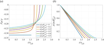
 $\beta =0$ surface inviscid case (figure 2a). The kinematic boundary condition (3.17) can then be integrated to obtain an explicit relation for the cavity radius as a function of time,
 \begin{equation} R_i(t) = \frac{2\eta}{{\rm \pi} \mu} \left[ \sqrt{1 +\frac{{\rm \pi} \gamma \mu (t^{*}-t)}{2\eta^{2}}}-1\right],\end{equation}
where  $t^{*} = (4\eta R_{i,0} + {\rm \pi}\mu R_{i,0}^{2})/(2\gamma ) = 2\tau _{1,0} + ({\rm \pi} /2)\tau _{2,0}$ is the closing time of the cavity written in terms of the initial radius
 $R_{i,0}=R_i(t=0)$ or the two initial time scales
 $\tau _{1,0}= \eta R_{i,0}/\gamma$ and
 $\tau _{2,0}=\mu R_{i,0}^{2}/\gamma$ (cf. the definitions of
 $\tau _1$ and
 $\tau _2$ in § 3.1). The area as a function of time is then
 ${\rm \pi} R_i(t)^{2}$; figure 2(b) shows the cavity area as a function of time as monolayer viscosity is varied. If (3.43) is substituted back into (3.42), we find an explicit relation for
 $F$ as a function of time:
 \begin{equation} F(t) ={-} \frac{\gamma}{{\rm \pi} \mu} \left[1 - \frac{1}{\sqrt{1 + {\rm \pi}\gamma\mu (t^{*}-t)/(2\eta^{2})}}\right]. \end{equation}
If  $\eta \to 0$ in this expression, we recover (3.41). On the other hand, fixing
 $\eta$ and expanding in small
 $(t^{*}-t)/\tau _{2,0}$ gives the result
 \begin{equation} F(t) ={-}\frac{\gamma}{{\rm \pi} \mu}\left[ \frac{{\rm \pi} \mu \gamma(t^{*}-t)}{4\eta^{2}} + \cdots\right] ={-}\frac{\gamma}{4\mu\beta_0^{2}} \frac{t^{*}-t}{\tau_{2,0}}+\cdots ,\end{equation}
where  $\beta _0 = \tau _{1,0}/\tau _{2,0}=\eta /(\mu R_{i,0})$, demonstrating the rapid variation of
 $F$ to zero as the cavity closes in the case of a viscous monolayer with small
 $\beta _0$ and regularising the singularity present in the inviscid model.
(a) The constant  $F$ from (3.42), which determines the rate of decrease of the cavity area, as a function of time for different values of the parameter
 $\beta _0=\eta /(\mu R_{i,0})$, with
 $R_{i,0}$ the cavity radius at
 $t=0$. Parameters:
 $\gamma = 0.01$,
 $\mu = 1$. Note that
 $F(t^{*})$ is not zero when
 $\eta =0$, whereas
 $F$ increases to zero linearly with a slope proportional to
 $\eta ^{-2}$ when
 $\eta >0$ and the hole radius is small compared with the Saffman–Delbrück length
 $\ell _{{SD}}=\eta /\mu$. (b) Increasing monolayer viscosity slows down the closing of the cavity. Parameters as in (a). The area of a sufficiently large cavity (i.e. one for which
 $\beta \ll 1$) initially decreases linearly in time with a slope described in (4.1). As the cavity radius becomes comparable to
 $\ell _{{SD}}$, the dynamics transition to a regime where
 $\beta$ is large and area changes quadratically in time, with
 $R_i$ scaling as in (4.2).

4. Comparison with experiments
The surface inviscid result of linearly decreasing area found by Alexander et al. (Reference Alexander, Bernoff, Mann, Mann and Zou2006) is a valid approximation for early times if monolayer viscosity is indeed small, as figure 2(a) illustrates. However, the predicted slope of  $-2\gamma /\mu$ does not hold as well for intermediate times in the presence of nonzero viscosity. The
 $O(\beta _0)$ perturbation to the slope at early times can be found by calculating
 \begin{equation} \left.\frac{\mathrm{d}A}{\mathrm{d}t} \right|_{t=0} = 2{\rm \pi} F|_{t=0} ={-}\frac{2\gamma}{\mu} \left(1 - \frac{2}{\rm \pi}\beta_0 + \cdots\right), \end{equation}
where we have taken  $\beta _0$ to be sufficiently small. Thus, the line tension value obtained from fitting data to the inviscid model is likely an underestimate.
In the opposite regime where the hole becomes sufficiently small and  $\beta \to \infty$, the viscous stress dominates, and (3.42) shows that
 $F\sim -\gamma /(2\mu \beta )$. Comparing this with (3.45) reveals
 \begin{equation} \frac{R_i}{R_{i,0}} \sim \frac{1}{2\beta_0} \frac{t^{*}-t}{\tau_{2,0}},\end{equation}
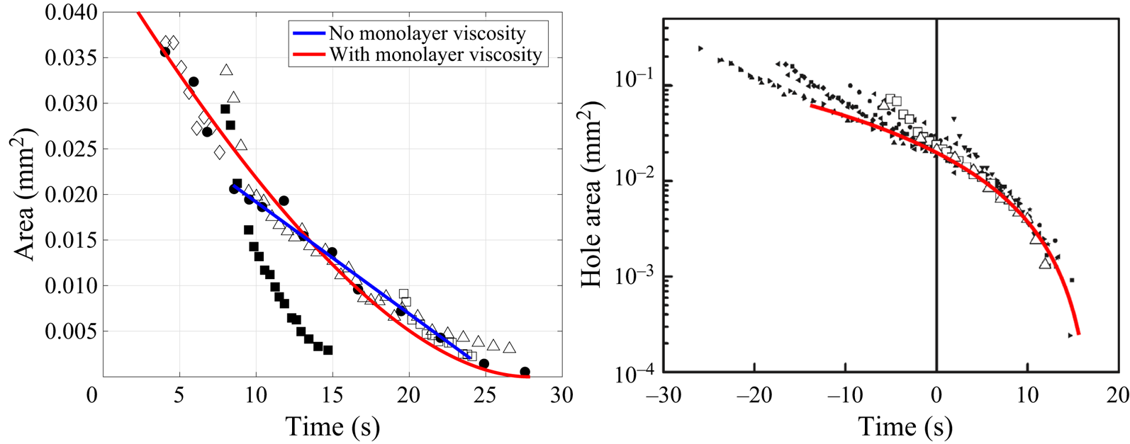
in this limit. That is, the cavity area changes quadratically with time in this regime, and the inviscid monolayer model consequently underestimates the closure time. The experimental data in Figure 6 of Alexander et al. (Reference Alexander, Bernoff, Mann, Mann and Zou2006) demonstrate a prominent quadratic-like slowing when the hole is small that may be representative of a monolayer viscosity. Figure 3(a) compares the authors’ original linear fit to the result of fitting to the modified area versus time relation using (3.43); the modification allows for a more accurate description of a broader range of data. The fit parameters were found to be a line tension of  $\gamma = 4.0\times 10^{-12}$ N and monolayer viscosity of
 $\eta = 3.2\times 10^{-7}$ kg s
 $^{-1}$, for the value of
 $\mu = 1.063\times 10^{-3}$ kg (m s)
 $^{-1}$ used in Alexander et al. (Reference Alexander, Bernoff, Mann, Mann and Zou2006). The corresponding Saffman–Delbrück length is
 $\ell _{{SD}} = 0.3$ mm, which gives a
 $\beta$ that is
 $O(1)$ at the initial time and confirms that the layer should not be treated as inviscid. We note that the value of
 $\eta$ obtained here is smaller than or comparable to the measured surface viscosity of other Langmuir monolayer systems (Joly Reference Joly1964; Barentin et al. Reference Barentin, Ybert, di Meglio and Joanny1999). Previous canal viscometer measurements have led to an estimate of
 $\eta \lesssim 10^{-8}$ kg s
 $^{-1}$ for PDMS monolayers (Jarvis Reference Jarvis1966).
(a) A reproduction of figure 6 of Alexander et al. (Reference Alexander, Bernoff, Mann, Mann and Zou2006) showing five different runs of experimental hole sizes as a function of time. As in the original paper, each run has been shifted horizontally to maximise overlap. The data are nonlinear when the hole becomes small, which could possibly be an effect of monolayer viscosity. The blue line is the linear fit that appeared in the paper originally; the red line is obtained by fitting the data to (3.43), which uses monolayer viscosity as an additional fit parameter and more accurately describes a broader range of data. The line tension and monolayer viscosity obtained from fitting are  $\gamma = 4.0\times 10^{-12}$ N and
 $\eta = 3.2\times 10^{-7}$ kg s
 $^{-1}$. (b) A reproduction of figure 4 from Zou et al. (Reference Zou, Bernoff, Mann, Alexander and Mann2010), comparing the same fit to (3.43) from (a) (continuous red line) and additional experimental data. In the original image, the experimental data were shifted in time to maximise overlap.

Figure 3(b) compares the same fit with the more recent experimental data from Zou et al. (Reference Zou, Bernoff, Mann, Alexander and Mann2010) (the experimental data in the original image were shifted horizontally to maximise overlap, whereas the continuous red line that appears is the exact same as that from figure 3a without any time shift); again, we see a strong agreement between the modified theory and the experiment.
5. Conclusion
Effectively, two regimes comprise the closing of a (sufficiently large) cavity in our model of a Langmuir film. The first is a tension-dominated regime where the area decreases linearly in time. This is followed by a viscosity-dominated regime where the area decreases quadratically in time just as the hole is about to close, effectively regularising the singularity. The two regimes can be delineated by the dimensionless parameter  $\beta$, which is a ratio of the Saffman–Delbrück length to the cavity radius.
We applied our simple theory to the experiments of Alexander et al. (Reference Alexander, Bernoff, Mann, Mann and Zou2006) and Zou et al. (Reference Zou, Bernoff, Mann, Alexander and Mann2010). By allowing for a monolayer viscosity in the model they proposed for the closing of a Langmuir film, the improved theory matches the original experiment more closely over a broader range of data. From fitting, we find a line tension of approximately 4.0 pN, which is the same order of magnitude as the previously reported values of  $0.69\pm 0.02$ pN from Zou et al. (Reference Zou, Bernoff, Mann, Alexander and Mann2010) and
 $1.1\pm 0.3$ pN from Mann, Hénon & Langevin (Reference Mann, Hénon and Langevin1992), but is different enough to see that the effects of monolayer viscosity are perhaps not as negligible for this system as the authors believed.
As mentioned previously, the vanishing of  $\eta$ from the bulk equations is a consequence of the symmetries of this particular problem. The effects of monolayer viscosity in a non-annular domain should be investigated as well; this is relevant to the problem at hand because it is difficult to experimentally create a perfectly circular cavity. The flow field of a disc-shaped monolayer of actively rotating colloidal magnets has also produced one example of an axisymmetric system where monolayer viscosity plays a non-trivial role in the bulk (Jia et al. Reference Jia, Irvine and Shelley2022); presumably there are many others. It would be interesting to study the effects of a surface viscosity on domain relaxation in non-axisymmetric Langmuir films, akin to the work done by Alexander et al. (Reference Alexander, Bernoff, Mann, Mann and Wintersmith2007), or to further generalise our model by adding a monolayer elasticity term.
Funding
M.J.S. acknowledges support by the National Science Foundation under awards DMR-1420073 (NYU MRSEC) and DMR-2004469.
Declaration of interest
The authors report no conflict of interest.