
1. Introduction
Real rough surfaces exhibit multi-scale, irregular and randomly distributed characteristics, and typically generate high Reynolds number wall-bounded turbulent flows. A pertinent example lies in ship boundary layer flows, where marine fouling organisms adhere to ship hulls, augmenting surface roughness and resistance to forward motion. Consequently, this leads to a notable decrease in sailing speed and a consequential rise in fuel consumption. Hence conducting in-depth research into the phenomena and mechanisms that distinguish rough-wall turbulence from smooth-wall turbulent boundary layer theory holds significant importance for accurately predicting and optimising the control of turbulent flows over rough surfaces in both natural and engineering applications.
The outer-layer similarity hypothesis (Townsend Reference Townsend1976) stands as a classical theory in studies of rough-wall turbulence. It suggests that at sufficiently high Reynolds numbers, the turbulent flow in the outer region is not influenced by the wall roughness, and exhibits similar behaviour to that of smooth-wall turbulence. However, universal criteria defining its applicability limits have not yet been fully established. In his review paper, Jiménez (Reference Jiménez2004) suggested that the ratio of the boundary layer thickness to the roughness height
 $\delta /k$
has to be at least 40, and the threshold Reynolds number
 $\delta ^+$
has to be at least 4000 for Townsend’s wall similarity hypothesis to be valid. Flack, Schultz & Shapiro (Reference Flack, Schultz and Shapiro2005) and Wu & Christensen (Reference Wu and Christensen2007) suggested using the ratio of the boundary layer thickness to the equivalent sand-grain roughness height
 $\delta /k_s \geqslant 40$
. In fact, most current studies on turbulent flow over rough walls are predominantly focused on the lower Reynolds number range, in which various factors such as dimensions, height and geometry of roughness elements and flow type may affect the outer-region turbulent flow (Bhaganagar, Kim & Coleman Reference Bhaganagar, Kim and Coleman2004; Lee & Sung Reference Lee and Sung2007; Volino, Schultz & Flack Reference Volino, Schultz and Flack2009; Hong, Katz & Schultz Reference Hong, Katz and Schultz2011; Chan et al. Reference Chan, MacDonald, Chung, Hutchins and Ooi2018). For example, Lee & Sung (Reference Lee and Sung2007) and Lee, Sung & Krogstad (Reference Lee, Sung and Krogstad2011) found that the introduction of two-dimensional rod and three-dimensional cube roughness both affected the turbulent Reynolds stresses not only in the roughness sublayer, but also in the outer region of the turbulent boundary layer (
 $\delta ^+=300{-}1400$
). The streaky structures and hairpin packets are significantly affected by surface roughness throughout the entire boundary layer. Choi et al. (Reference Choi, Hwang, Lee and Lee2020) further investigated the effects of the roughness height in turbulent boundary layers over rod- and cuboid-roughened walls, and the outer layer similarity between the flows over the rough and smooth walls is found only when
 $\delta / k \geqslant250$
and
 $\delta / k \geqslant100$
for the two-dimensional rod and three-dimensional cuboid, respectively. Bhaganagar et al. (Reference Bhaganagar, Kim and Coleman2004) investigated the influence of three-dimensional egg-carton roughness on the outer-region turbulent flow in an asymmetric channel (
 $\delta ^+=400$
), and found that the velocity fluctuations are altered by roughness in the outer region, and the vorticity fluctuations are not significantly altered. There is interaction between the inner and outer layers of the rough-wall turbulent boundary layer at the large scales, and roughness enhances the wall-normal transport via the transport terms of the Reynolds stress budgets. Chan et al. (Reference Chan, MacDonald, Chung, Hutchins and Ooi2018) and Ma et al. (Reference Ma, Xu, Sung and Huang2023) also studied turbulent flow over three-dimensional egg-carton rough surfaces at friction Reynold number 540, but in symmetric channel and pipe models, and found that the outer-layer similarity relationship of statistical quantities, such as velocity deficit and Reynolds stress profiles, coincides well in the outer region with that observed in smooth-wall conditions. From the above, conflicting opinions on outer-layer similarity persist in the literature for turbulent flow over rough walls. It is critical to ascertain whether various laws, properties and theories obtained based on smooth-wall assumptions can be applied to rough-wall turbulent flows.
Coherent structures play a crucial role in both the initiation and development of wall turbulence, greatly influencing the transport of mass, momentum and energy within turbulent flow. Over time, researchers have gained a relatively deep understanding of the kinematic and dynamic characteristics of coherent structures in smooth-wall turbulence through numerical simulations, theoretical analysis and experiments (Jiménez Reference Jiménez2018). In the near-wall region, typical coherent structures include quasi-streamwise vortices and low-speed streaks, which are important constituents of the near-wall self-sustaining process (Hamilton, Kim & Waleffe Reference Hamilton, Kim and Waleffe1995; Jiménez & Pinelli Reference Jiménez and Pinelli1999). In high-Reynolds-number wall turbulence, large-scale motions and very-large-scale motions emerge within the logarithmic and outer regions, which exert modulation and superimposition effects on turbulent fluctuations in the near-wall region (Hutchins & Marusic Reference Hutchins and Marusic2007; Mathis, Hutchins & Marusic Reference Mathis, Hutchins and Marusic2009; Marusic, Mathis & Hutchins Reference Marusic, Mathis and Hutchins2010). Indeed, the presence of wall roughness alters the pre-existing coherent structures in the turbulent boundary layer, resulting in more complex flow patterns. The alterations are significantly influenced by the topological characteristics of the surfaces involved. For instance, velocity streaky structures near the wall persist but are abruptly disrupted by two-dimensional roughness, while they may meander around three-dimensional roughness elements. Additionally, the streamwise lengths of these structures tend to decrease in the presence of roughness. The morphological characteristics of vortical structures, such as tilt angles, sizes and distribution patterns, also undergo changes compared to smooth-wall turbulence (Flores & Jimenez Reference Flores and Jimenez2006; Lee et al. Reference Lee, Sung and Krogstad2011; De Marchis, Milici & Napoli Reference De Marchis, Milici and Napoli2015). Hong et al. (Reference Hong, Katz and Schultz2011) discovered that roughness-scale eddies are transferred from the near-wall region to the outer region through the convection of large-scale structures, which makes the outer region contain more small-scale energy, and viscous dissipation effects are enhanced. In addition, spanwise heterogeneity in the roughness can induce the generation of large-scale secondary flows that manifest as high-momentum pathways (HMPs) and low-momentum pathways (LMPs) in the streamwise velocity (Barros & Christensen Reference Barros and Christensen2014). It is widely accepted that the secondary flow of the Prandtl second kind is induced by turbulence anisotropy, as reviewed by Nikitin, Popelenskaya & Stroh (Reference Nikitin, Popelenskaya and Stroh2021). The spanwise spacing and relative surface elevation of roughness elements can affect the intensity and direction of these secondary flows (Vanderwel & Ganapathisubramani Reference Vanderwel and Ganapathisubramani2015; Medjnoun, Vanderwel & Ganapathisubramani Reference Medjnoun, Vanderwel and Ganapathisubramani2018; Yang & Anderson Reference Yang and Anderson2018; Stroh et al. Reference Stroh, Schäfer, Frohnapfel and Forooghi2020; Wangsawijaya et al. Reference Wangsawijaya, Baidya, Chung, Marusic and Hutchins2020; Zampiron, Cameron & Nikora Reference Zampiron, Cameron and Nikora2020). Secondary flows can lift large-scale turbulent eddies from the near-wall region and suppress coherent structures, leading to alterations in the statistical properties of turbulence in both inner and outer regions, but the specific underlying mechanisms are still lacking in the literature.
In rough-wall turbulent flows, direct numerical simulations (DNS) have become a critically important method for the investigation of turbulence physics, which can effectively acquire flow information within the roughness sublayer and outer region. Roughness is modelled by volume forces or explicitly described by body-fitted grids (Chung et al. Reference Chung, Chan, MacDonald, Hutchins and Ooi2015). Researchers have generally focused on regular roughness characterised by similar-shaped and regularly distributed roughness elements or sinusoidal waves (Bhaganagar et al. Reference Bhaganagar, Kim and Coleman2004; Orlandi & Leonardi Reference Orlandi and Leonardi2006, Reference Orlandi and Leonardi2008; Lee et al. Reference Lee, Seena, Lee and Sung2012; Seddighi et al. Reference Seddighi, He, Pokrajac, O’Donoghue and Vardy2015). Flow behaviour over regular roughness is often more predictable due to the regularity of the surface features, facilitating analysis and modelling. However, the flow behaviour and properties over regular roughness and random roughness may exhibit significant differences, but it remains unclear which conclusions drawn from the regular roughness are applicable to flow over random roughness. During the past decade, there were a significant number of DNS studies on irregular roughness; see the review paper by Chung et al. (Reference Chung, Hutchins, Schultz and Flack2021) and more recent examples of DNS investigations, including Jelly et al. (Reference Jelly, Ramani, Nugroho, Hutchins and Busse2022), Sarakinos & Busse (Reference Sarakinos and Busse2022), Womack et al. (Reference Womack, Volino, Meneveau and Schultz2022), Busse & Jelly (Reference Busse and Jelly2023), Dunbar, Scandura & O’Donoghue (Reference Dunbar, Scandura and O’Donoghue2023), Kaminaris et al. (Reference Kaminaris, Balaras, Schultz and Volino2023) and Narayanan et al. (Reference Narayanan, Singh, Nauer, Belt, Palermo and Lakehal2024). For example, Thakkar, Busse & Sandham (Reference Thakkar, Busse and Sandham2017) conducted DNS to investigate the rough-wall flow over an irregular industrial grit-blasted surface, and established higher-order drag scaling models by considering more roughness parameters for this realistic random roughness. The characteristics of rough surfaces can be more accurately captured by multiple parameter coupling, thereby improving the applicability and reliability of scaling models. Yuan & Piomelli (Reference Yuan and Piomelli2014) investigated the roughness effects on turbulent flows within the roughness sublayer through DNS, and the rough surfaces were generated by randomly rotated ellipsoids. The energy transfer between the roughness-induced velocity fluctuation and the turbulent velocity fluctuation is then revealed by the Reynolds stress budgets after the triple decomposition. Sarakinos & Busse (Reference Sarakinos and Busse2019, Reference Sarakinos and Busse2022, Reference Sarakinos and Busse2024) used an algorithm that mimics the settlement behaviour of barnacles to generate barnacle-type rough surfaces, and performed DNS to investigate the influence of rough surfaces with increasing clustering, coverage and Reynolds number on wall-bounded turbulence. The mean velocity and stress profiles are affected by variations in these parameters. The partial recovery of smooth-wall behaviour over the smooth sections of the barnacle surface can be observed in the Reynolds stress statistics. Womack et al. (Reference Womack, Volino, Meneveau and Schultz2022) and Kaminaris et al. (Reference Kaminaris, Balaras, Schultz and Volino2023) conducted DNS and experiments on turbulent boundary layer flow over regularly and irregularly arranged barnacle rough surfaces by varying the planform densities. Differences between regular and random surface flow parameters were due to the presence of secondary flows. Secondary flows were primarily present over the random surfaces, and not discernible or very weak over the regular surfaces, which is closely related to the leading edge of the roughness.
Since random roughness is more common on both engineering and natural surfaces than regular roughness, this paper enriches this numerical research. The present work aims to examine the interaction between large-scale structures induced by roughness and outer large-scale structures from the perspective of inter-scale energy transport. The DNS were performed for a fully developed turbulent open-channel flow over six different arrangements of rough surfaces at a moderate friction Reynolds number, i.e.
 $Re_{\tau } \approx 540$
. A triple decomposition was adopted to extract turbulent fluctuations from coherent fluctuations that arise due to the presence of roughness. Subsequently, mean velocity profiles, stress profiles, and one-dimensional pre-multiplied energy spectra were scrutinised, and the results were compared with those obtained from smooth-wall cases for comparative analysis. Large-scale secondary flows induced by roughness were identified in the spanwise energy spectra of streamwise velocity fluctuations, evident in both instantaneous snapshots and time-averaged flow fields. Furthermore, spectral analysis of the two-point correlation transport equation and triadic interaction analysis were performed to reveal the inter-scale turbulent energy transfer process in the presence of differently arranged rough walls. These analyses shed light on how secondary flows impact the outer-layer similarity of turbulence statistics and coherent structures. The rest of this paper is organised as follows. The problem formulation and numerical method are briefly introduced in § 2. The effects of roughness on turbulence statistics and coherent structures, and a detailed analysis of roughness-induced secondary flows and interactions with large-scale structures, are presented in § 3. Finally, conclusions are drawn in § 4.
2. Problem formulation
The problem considered here is a fully developed three-dimensional open-channel turbulent flow over rough walls. A sketch of the computational domain and coordinate system is shown in figure 1. The flow is driven by an averaged streamwise gradient of pressure that is dynamically adjusted and makes the flow rate strictly constant in time. A right-handed Cartesian coordinate system is adopted, with the
 $x$
,
 $y$
and
 $z$
axes (also denoted as
 $x_1$
,
 $x_2$
and
 $x_3$
for the tensor notation) being the streamwise, vertical and spanwise directions, respectively. The prescribed rough surface is generated by the cosine function. Assuming that
 $(x_0,z_0)$
is the centre of a single roughness element, the deformation is described according to
 \begin{equation} {\eta }_{d}(x, z)=k\left (1+\cos \frac {\unicode{x03C0} r(x, z)}{R_{0}}\right ), \quad \left (x-x_{0}\right )^{2}+\left (z-z_{0}\right )^{2} \leqslant R_{0}^{2}, \end{equation}
where
 ${\eta }_{d}(x, z)$
denotes the rough surface elevation,
 $r(x,z)=\sqrt { (x-x_{0} )^{2}+ (z-z_{0} )^{2}}$
, and
 $k$
and
 $R_0$
denote the central depth and radius of the roughness elements, respectively. The resolvable turbulent flow field is described by the filtered incompressible Navier–Stokes equations and the continuity equation:
 \begin{equation} \frac {\partial u_{i}}{\partial t}+u_{j} \frac {\partial u_{i}}{\partial x_{j}}=-\frac {\partial p}{\partial x_{i}}+\frac {1}{R e_{b}} \frac {\partial ^{2} u_{i}}{\partial x_{j}\, \partial x_{j}}, \end{equation}
 \begin{equation} \frac {\partial u_{i}}{\partial x_{i}}=0, \end{equation}
where
 ${u_i}\ ( i=1,2,3 )=( u, v, w )$
are the velocity components in the three directions
 $x_i\ ( i=1, 2, 3 )=( x, y, z )$
,
 $p$
is the pressure, and
 $R e_{b}=U_b \delta / \nu$
is the bulk Reynolds number denoted by the bulk velocity
 $U_b$
, open-channel height
 $\delta$
, and kinematic viscosity
 $\nu$
. The bulk velocity is defined as
 $U_b=Q/\delta$
, where
 $Q$
denotes the volume flow rate per unit spanwise length, and the open-channel height
 $\delta$
is defined as the vertical distance from the bottom wall to the top boundary. Correspondingly, the friction Reynolds number is
 $R e_{\tau }=u_{\tau } \delta / \nu$
, where
 $u_{\tau }$
is the characteristic friction velocity defined as
 ${u_{\tau }}=\sqrt { {{\tau }_{w}}/\rho }$
, and
 $\tau _w$
is the temporally and spatially averaged total drag at the rough surface. This encompasses both friction drag and pressure drag components. Throughout this paper, the superscript ‘+’ denotes quantities scaled by wall viscous unit. For instance,
 $u^+ = u / u_{\tau }$
represents the velocity scaled by the friction velocity, and
 $y^+ = y u_{\tau } / {\nu }$
denotes the height scaled by the viscous length scale.
Schematic diagram of turbulent channel flow over a random rough wall.

The DNS of the turbulent flow are carried out using a computational coordinate system based on a boundary-fitted grid system in Cartesian coordinates (
 $t$
,
 $x$
,
 $y$
,
 $z$
) in physical space, by adopting an algebraic mapping, i.e.
 \begin{equation} t=\tau , \quad x_{1}=\xi _{1}, \quad x_{2}=\xi _{2}\left(1-\frac{\eta _{d}}{\delta} \right)+\eta _{d}, \quad x_{3}=\xi _{3}, \end{equation}
where
 $\xi _{1}$
,
 $\xi _{2}$
,
 $\xi _{3}$
and
 $\tau$
are the space and time coordinates in the computational domain. Next, (2.2) and (2.3) are reformulated in terms of the curvilinear coordinates (
 $\tau$
,
 $\xi _{1}$
,
 $\xi _{2}$
,
 $\xi _{3}$
) in the computational space (Ge, Xu & Cui Reference Ge, Xu and Cui2010). For spatial discretisation, the pseudo-spectral method is applied in the
 $\xi _{1}$
and
 $\xi _{3}$
directions, along with the second-order finite-difference scheme on the staggered grids in the
 $\xi _{2}$
direction. For time advancement, the third-order time-splitting method is applied.
In our simulation, a free-slip wall boundary condition is enforced at the top boundary, and a no-slip boundary condition is imposed at the bottom boundary of the computational domain. Periodic boundary conditions are enforced in the streamwise and spanwise directions. Six sets of rough-wall configurations were simulated, each corresponding to different arrangements of roughness. Additionally, results from the open-channel flow with a smooth wall are included for comparative analysis. A summary of the flow and roughness parameters is listed in table 1. In the table,
 $k_{a}^+$
is the mean roughness element height,
 $k_{rms}^+$
is the root mean square roughness height,
 $k_{max}^+$
is the maximum height of roughness elements, and
 $k_{min}^+$
is the minimum height of roughness elements. Also,
 $\lambda _f$
is the ratio of the total projected frontal area of roughness elements to the total plane area (namely the frontal solidity; see review by Chung et al. Reference Chung, Hutchins, Schultz and Flack2021), and
 $\lambda _p$
is the ratio of the total plane area of roughness elements to the total plane area. The rough surfaces for cases R1–R4 are generated using the same set of roughness elements, thus the height and density parameters are the same. Here,
 $\lambda _x/ \delta$
(
 $\lambda _z/ \delta$
) is the main wavenumber scale obtained by the streamwise (spanwise) Fourier transform of the spanwise (streamwise) average rough surface height. Smooth paths are defined where the streamwise-averaged rough surface height is less than 0.5 wall viscous unit, and their spanwise proportion
 $\gamma _s$
is then calculated (Stroh et al. Reference Stroh, Schäfer, Frohnapfel and Forooghi2020). A Voronoï-diagram-based analysis method (Nilsen, Andersson & Zhao Reference Nilsen, Andersson and Zhao2013) is applied to quantitatively assess the clustering characteristics of roughness elements on the surface. By extracting the minimum and maximum Voronoï cell areas (
 $A_{min}$
and
 $A_{max}$
), as well as the standard deviation of the cell areas (
 $std$
), the degree of clustering can be characterised effectively. The Voronoï diagrams corresponding to the six different roughness arrangements are provided in Appendix A. Local roughness clustering can result in the formation of small Voronoï cells and an increased
 $std$
in cell areas. For the regular arrangement with a fully uniform distribution,
 $std$
is zero, and
 $A_{min}/A_{max}$
reaches its maximum value 1.
Flow and roughness parameters.

In all the simulations, the friction Reynolds number
 $Re_{\tau }$
is approximately 540. The computational domain size is
 ${L_x}\times {L_y}\times {L_z}=4\unicode{x03C0} \delta \times \delta \times 2\unicode{x03C0} \delta$
. A grid-independence test is done with grid numbers
 $288\,\times \,192\,\times \,288$
(M1),
 $576\,\times \,192\,\times \,576$
(M2) and
 $1152\,\times \,288\,\times \,1152$
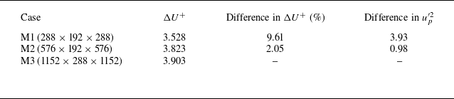
(M3) for the R1 case. Table 2 shows no significant difference in the roughness function and the peak streamwise Reynolds stress between M2 and M3, where the roughness function
 $\Delta U^+$
is calculated by the mean downward shift of the streamwise velocity profile within the range
 $y^+=100{-}200$
. Therefore, M2 is adopted for the following simulations. Correspondingly, the grid sizes in the streamwise and spanwise directions are uniform with resolutions of
 $\Delta x^{+}\approx 11.78$
and
 $\Delta z^{+}\approx 5.89$
, respectively. The grid points along the
 $y$
axis follow a cosine distribution with
 $\Delta y _{min }^{{+}}\approx 0.02$
near the bottom boundary and
 $\Delta y _{max }^{{+}}\approx 4.4$
near the top boundary. For each roughness element, approximately 20–26 and 40–52 grid points are typically used in the streamwise and spanwise directions, respectively. Statistics are obtained from 800 instantaneous flow field data, with an interval of approximately 20 viscous time units after statistically steady state has been reached, corresponding to more than 60 flow-through times, to ensure that the presented results are statistically converged (Hwang & Lee Reference Hwang and Lee2018; Stroh et al. Reference Stroh, Schäfer, Frohnapfel and Forooghi2020).
Grid-independence test for the R1 case.

3. Results and discussion
3.1. Roughness effect on turbulence statistics
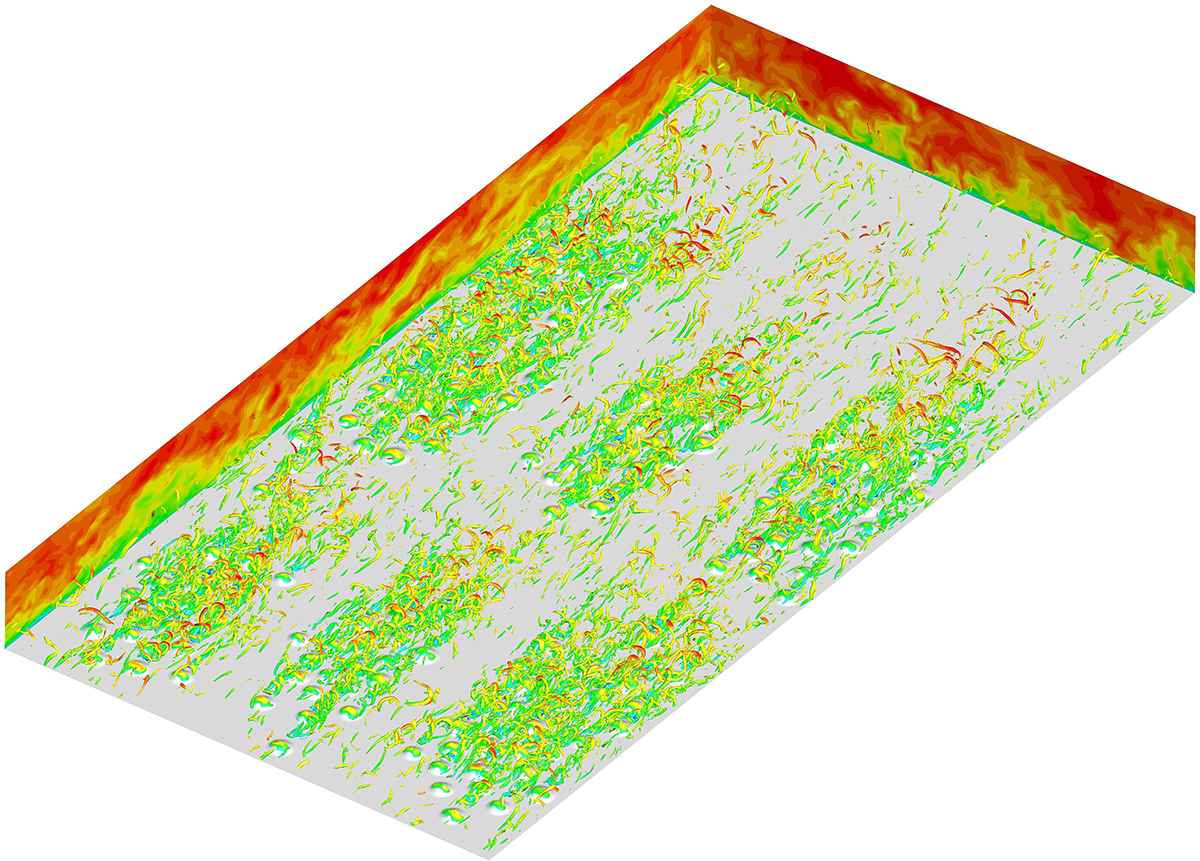
A sketch of the instantaneous turbulent flow fields over rough walls is shown in figure 2, providing an intuitive depiction of the relationship between the distribution of vortical structures and the roughness geometry. The overlying vortical structures are visualised by the iso-surface of swirling strength
 $\lambda _{ci}$
and coloured by the streamwise velocity. In all rough-wall cases, the vortical structures are dominated by quasi-streamwise vortices, but they exhibit significant differences due to variations in roughness arrangements. As shown in figure 2(a,b,c), clusters of vortical structures densely form in regions where roughness elements aggregate, whereas they are relatively sparse over the smooth-wall region. Conversely, the distribution of vortical structures appears relatively more uniform for the R4 case with homogeneous random arrangements and the staggered case, as shown in figure 2(d,e). The vortical structures exhibit alignment and clustering along the flow direction for the regular case, as shown in figure 2(f). From figure 2, we can see that the presence of roughness elements introduces complexity to the flow passage, culminating in a turbulent flow field characterised by abundant swirling motions. The streamwise velocity contour plots in the
 $x{-}y$
plane exhibit downstream tilting in the near-surface region, which is consistent with the morphology of streamwise vortices. Moreover, the streamwise velocity contour plots in the
 $y{-}z$
plane show the formation of large-scale streaky structures, with the wake region of the roughness elements corresponding to low-speed zones. To study more quantitatively the effects of roughness arrangements, the turbulence statistics are presented and discussed in the subsections below.
Instantaneous vortical structures over rough walls together with the streamwise velocity on the
 $x{-}y$
and
 $y{-}z$
cross-sections. The vortical structures are displayed by the iso-surface
 $\lambda _{ci}=10$
and coloured by the instantaneous streamwise velocity. Corresponding rough-wall cases are: (a) R1 clustering
 $2\times3$
, (b) R2 clustering
 $3\times2$
, (c) R3 clustering 2/1/3, (d) R4 randomly homogeneous, (e) staggered and (f) regular.

Profiles of (a) the mean streamwise velocity plotted against the wall-normal height
 $(\bar {y}-y_0)^+$
, and (b) the velocity defects plotted against the wall-normal height normalised by the half-channel height
 $(\bar {y}-y_0)/ (\delta -y_0)$
. In the abscissa axis,
 $\bar {y}$
represents the mean vertical distance from the wall in the boundary-fitted curvilinear coordinate system, and
 $y_0$
represents the location of the roughness mean plane (i.e.
 $y_0 / \delta=0.0035$
for the R1–R4 cases, and
 $y_0 / \delta=0.0031$
for the staggered and regular cases, respectively). Dashed lines show
 $U^+=\bar {y}^+$
and
 $U^+=1/\kappa \ln (\bar {y}^+)+C$
, for
 $\kappa=0.4$
and
 $C= 5.3$
. The vertical dashed and dash-dotted lines represent the maximum roughness element height for the R1–R4 cases, and for the staggered and regular cases, respectively.

In a rough-wall turbulent flow, knowledge of the virtual origin (
 $y=0$
) is critical for the ability to compare turbulence statistics for different surfaces. The virtual origin depends on roughness geometry, and a widely used method is to set the mean roughness height of each surface to zero by applying a small offset
 $y_0$
to the smooth wall (Thakkar et al. Reference Thakkar, Busse and Sandham2017; Sarakinos & Busse Reference Sarakinos and Busse2022; Jensen & Forooghi Reference Jensen and Forooghi2025). Figure 3 shows the mean streamwise velocity profiles and velocity defects in semi-logarithmic coordinates for various roughness arrangements, with an inset illustrating an enlarged view of the logarithmic region
 $100\leqslant (\bar {y}-y_0) ^+ \leqslant200$
. The plane-averaged results are obtained in the boundary-fitted coordinate system (Ma et al. Reference Ma, Xu, Sung and Huang2023). Roughness induces a downward shift in the mean velocity profiles compared to that of the smooth-wall case, but all the mean velocity profiles still adhere to the logarithmic law. From the inset, it can be observed that some profiles have slightly different slopes in the shown log layer, e.g. the staggered case profile. By plotting the velocity defects in figure 3(b), the profiles show a good collapse of the R4 and regular cases with the smooth-wall case above
 $(\bar {y}-y_0) / \delta \approx 0.2$
, while for the other rough-wall cases, a higher wall-normal position is required to achieve similarity in the outer region, i.e.
 $(\bar {y}-y_0) / \delta \gt 0.7$
. Therefore, from the perspective of first-order mean statistics, the hypothesis of outer-layer similarity (Townsend Reference Townsend1976) is retained for rough-wall flows.
The downward shift (i.e. the roughness function
 $\Delta U^+$
) is obviously influenced by roughness arrangements. For the R4 case with the homogeneous random arrangement,
 $\Delta U^+$
is larger than those of R1–R3 with the aggregated arrangements. As shown in table 1,
 $A_{min}/A_{max}$
also reflects that cases R1–R3 have similar degrees of clustering, whereas the rough distribution of R4 is relatively more dispersed. For the staggered case, the profile is more similar to that of the random arrangement, resulting in the largest
 $\Delta U^+$
. These findings are consistent with the conclusions of Sarakinos & Busse (Reference Sarakinos and Busse2019). In their previous studies, the barnacle-type rough surfaces with three different levels of clustering could be well characterised by the current
 $A_{min}/A_{max}$
or
 $std$
. As the degree of clustering decreases,
 $\Delta U^+$
increases, and when beyond a certain value,
 $\Delta U^+$
tends to converge. The discrepancy in
 $\Delta U^+$
between clustered and dispersed roughness configurations mainly stems from the fact that clustered roughness enhances the sheltering effect; i.e. roughness elements within a cluster that have upstream neighbours are exposed to lower mean streamwise velocity. For case R4, almost all roughness elements have their own distinct wake patterns, with a small area of low streamwise velocity on the downstream side. It is worth noting that the
 $\Delta U^+$
values of the three clustered roughness cases exhibit significant differences, which are related to the arrangement of the roughness clusters. The presence of the streamwise smooth-wall region facilitates more low-resistance paths, thereby decreasing
 $\Delta U^+$
, as evidenced by
 $\gamma _s$
in table 1. For the R2 case, the largest
 $\gamma _s$
results in the smallest
 $\Delta U^+$
; the R1 and R3 cases have relatively smaller
 $\gamma _s$
, corresponding to larger
 $\Delta U^+$
. Also for the regular case,
 $\Delta U^+$
is slightly smaller than that of the staggered case due to the presence of low-resistance paths. Furthermore, the standard deviation (see table 1) of the Voronoï cell areas can also approximately reflect these arrangement characteristics. For example, there are large Voronoï cells forming in the smooth-wall regions between the roughness clusters for R2, and
 $std$
is relatively small. For R1, larger Voronoï cells are more likely to form by connecting with the boundaries, yielding a larger
 $std$
. The
 $std$
shows a decreasing trend from clustered roughness (R1–R3) to dispersed roughness (R4), and then to a regular or staggered arrangement. Therefore, the effect of roughness arrangement on the roughness function
 $\Delta U^+$
can be attributed to the degree of clustering and the proportion of smooth paths. The variation in the mean velocity profile reflects the influence of roughness elements on turbulent wall resistance (Ma et al. Reference Ma, Xu, Sung and Huang2020). For rough-wall flows, the total wall resistance is composed of pressure and viscous drag components, with the latter including viscous shear stress
 $-\nu\, \mathrm{d}U^+/\mathrm{d}y^+$
and Reynolds shear stress. The arrangement of roughness elements has different effects on the dispersive Reynolds shear stress, which will be discussed in detail below. We expect that the degree of clustering would have a much stronger influence for sparse rough surfaces, and the relationship between aggregation parameter and wall resistance would be explored in future work.
In smooth-wall turbulence, the Reynolds decomposition is applied to decompose a physical quantity into its mean and fluctuating components,
 \begin{equation} u_i(x, y, z, t)=\bar {u}_{i}(x,y,z)+u'_i(x, y, z, t), \end{equation}
where
 $\bar {u}_{i}$
is the time-averaged mean (the overline denotes temporal averaging), and
 $u'_i$
is the fluctuation about the time-averaged mean. However, in turbulent flow over a rough surface, it is imperative to consider the fluctuations caused by the surface irregularities when examining the flow data. To address this, we adopt a triple decomposition method derived from the Reynolds decomposition (Raupach & Shaw Reference Raupach and Shaw1982; Nikora et al. Reference Nikora, Goring, McEwan and Griffiths2001, Reference Nikora, McEwan, McLean, Coleman, Pokrajac and Walters2007), i.e.
 \begin{equation} u_i(x, y, z, t)={U_i}(y)+\tilde {u}_i(x, y, z)+u_i^{\prime \prime }(x, y, z, t), \end{equation}
where
 $U_i=\langle \bar {u}_i\rangle$
is the spatial and temporally averaged mean, which is also known as the global mean (
 $\langle \cdot\rangle$
denotes spatial averaging),
 $\tilde {u}_i=\bar {u}_i-U_i$
is the spatial variation of time-averaged flow around individual roughness elements and is defined as the coherent or dispersive component, and
 $u_i^{\prime \prime }$
is the turbulent fluctuation. When considering the global mean, the sum of
 $\tilde {u}_i$
and
 $u_i^{\prime \prime }$
is the total velocity fluctuation
 $u'_i$
(i.e.
 $\tilde {u}_i+u_i^{\prime \prime }=u'_i$
), which contains both the coherent and turbulent fluctuation components. Accordingly, the second-order velocity correlation can be decomposed into the mean, dispersive and turbulent Reynolds stresses, as
 \begin{equation} \overline {u_{i} u_{j}}=\overline { \big({U}_{i}+\tilde {u}_{i}+u_{i}^{\prime \prime }\big) \big({U}_{\!j}+\tilde {u}_{\!j}+u_{j}^{\prime \prime } \big)}={U}_{i} {U}_{\!j}+\overline {\tilde {u}_{i} \tilde {u}_{\!j}}+\overline {u_{i}^{\prime \prime } u_{j}^{\prime \prime }}. \end{equation}
Profiles of the Reynolds stresses of total fluctuations: (a) streamwise component, (b) vertical component, (c) spanwise component and (d) shear stress, plotted against the wall-normal height
 $\bar {y}^+$
. The definitions of the line colours and line types are the same as those in figure 3.

Similar methods are also applied in the analysis of flow over rough surfaces with uneven distributions, such as plant canopy flows (Raupach & Shaw Reference Raupach and Shaw1982) and open-channel flow over rough beds (Nikora et al. Reference Nikora, Goring, McEwan and Griffiths2001, Reference Nikora, McEwan, McLean, Coleman, Pokrajac and Walters2007). The Reynolds stress profiles of total velocity fluctuations are plotted in figure 4 for the streamwise, vertical, spanwise and shear stress components, respectively. The profiles are obtained by the global mean on a curved plane of the boundary-fitted grid and over time. In the smooth-wall case, the streamwise Reynolds normal stress attains its peak at
 $(\bar {y}-y_0)^+ \approx15$
(figure 4
a). This peak corresponds to the near-wall cycle, where organised coherent structures are observed. The presence of roughness elements elevates this wall-normal location by approximately a viscous-scaled roughness height, with the peak intensity slightly exceeding that of the smooth-wall result. The disparities among different roughness arrangements manifest in the outer region of the streamwise stress profiles, corresponding to new large-scale production and scale interactions occurring in this region, which are detailed in § 3.3. The outer regions of the wall-normal stress and shear stress components closely resemble those of the smooth-wall turbulence, exhibiting less influence from the rough wall (figure 4
b,d). But the outer region of the spanwise stress component is affected by roughness elements (figure 4
c). In the near-wall region, the wall-normal and spanwise Reynolds stresses are both larger than the smooth-wall result, associated with the uplift of streamwise vortices above the roughness elements (De Marchis et al. Reference De Marchis, Milici and Napoli2015). The shear stress component shows prominent negative regions in the near-wall region, corresponding to the presence of strong negative momentum flux near the windward and leeward sides of the roughness elements.
Contours of the one-dimensional pre-multiplied spanwise energy spectra of streamwise velocity total fluctuation for the rough- and smooth-wall cases: (a) R1 clustering
 $2\times3$
, (b) R2 clustering
 $3\times2$
, (c) R3 clustering 2/1/3, (d) R4 randomly homogeneous, (e) staggered and (f) regular. Black solid lines represent the contours of rough-wall energy spectra, and the red cloud diagram represents the smooth-wall case. The vertical red solid line represents the spanwise scale
 $\lambda _z / \delta$
of rough surfaces, and the two horizontal black dashed lines represent the maximum and minimum heights of the roughness elements, respectively.

One-dimensional pre-multiplied spanwise energy spectra of streamwise velocity total fluctuations are shown in figure 5 for various rough-wall cases together with the smooth-wall case. The spectral analysis provides a better representation of the dominant wavelengths of the turbulent structures. From the energy spectra of smooth-wall turbulence, two peaks can be observed in the spectra that correspond to the inner/outer scale separation even at a friction Reynolds number
 $Re_\tau \approx 540$
. The inner peak is located at
 $\bar {y}^+ \approx 15$
, whereas the outer peak is located at
 $\bar {y}^+ \approx 150$
. In comparison to previously studied sinusoidal roughness (Ma et al. Reference Ma, Xu, Sung and Huang2023), the roughness form examined in this paper has a relatively minor effect on the peaks observed in the inner region of the spanwise energy spectra. No significant weakening of peak intensity or alteration in elevation has been observed. Nevertheless, the multi-scale effects of roughness elements are evident in the inner spectral peaks. Simultaneously, the independent fundamental and harmonic components caused by roughness periodicity exist in the spectra for the regular and staggered cases.
Compared to the inner region, roughness arrangements cause more obvious differences in the outer region of the energy spectra. For R1–R3, larger-scale secondary-flow structures emerge in the outer region when turbulent flows interact with aggregated roughness. Additionally, the intensity, scale and vertical height of the outer peak vary among configurations for R1–R3. For the R1 case in figure 5(a), the large-scale spectral peak is located at the spanwise scale
 $\lambda _z^+ \approx 1120$
and the wall-normal height
 $\bar {y}^+ \approx 220$
. For the R2 case in figure 5(b), the large-scale spectral peak is located at the spanwise scale
 $\lambda _z^+ \approx 1680$
and the wall-normal height
 $\bar {y}^+ \approx 320$
. It can be seen that the scale of the peak is close to the main scale
 $\lambda _z / \delta$
of the roughness height distribution along the spanwise direction, as listed in table 1. This phenomenon suggests that the spanwise heterogeneity of roughness is directly related to the energy distribution of the secondary flow in the outer region. Here, the spanwise heterogeneity refers to the status that the adjacent patches of relatively high and low roughness elements both exist in the
 $y{-}z$
plane. The large-scale spectral peak corresponding to secondary flows is not obvious in the R4 case (figure 5
d), and in the R3 case (figure 5
c), the peak is significantly weaker than in the R1 and R2 cases, with its spanwise scale and normal height more closely resembling those of the R2 case. One possible reason is that secondary flows are barely generated for the R3 and R4 cases due to the weak spanwise heterogeneity. For example, the R3 case has roughness clusters at the middle of rough surface, which greatly reduces the spanwise heterogeneity of roughness compared to R2. Another possible reason is insufficient resolution in the high-wavelength (low-wavenumber) region. To achieve good resolution in this region, the spanwise width of computational domain should be significantly increased, making DNS extremely expensive. As shown in figure 5(e,f), the spanwise spacing of the regular and staggered roughness is fixed and relatively small, where no secondary flow is observed. However, the large-scale spectral peak of the outer region for the regular case is enhanced, and the length scale increases, whereas there is an opposite change for the random arrangement. Note that while the length scales of the large-scale spectral peak for the R1 case and the regular case in the outer region are very similar, their underlying causes are different. The former corresponds to the scale of secondary flow, whereas the latter corresponds to the enhancement of large-scale structures in the outer region, as will be confirmed later. Additionally, it is evident from the figure that the outer peaks for the R1 case and the regular case extend deeply into the near-wall region, thus affecting the large-scale structures in the near-wall region. The comparison of spectral peaks between smooth- and rough-wall cases effectively reveals the influence of roughness. Roughness disrupts the outer-layer similarity of energy spectra, altering the distribution of energy at large scales, especially the generation of secondary flows. The key question for further investigation is how the secondary-flow structures interact with the original large-scale structures in the outer region.
Normalised one-dimensional pre-multiplied spanwise energy spectra of streamwise velocity total fluctuations for the rough- and smooth-wall cases at (a)
 $\bar {y}^+=25$
and (b)
 $\bar {y}^+= 280$
. The vertical black dashed lines represent the spanwise scale
 $\lambda _z/\delta$
of rough surfaces.

As discussed above, the spectral peak for the current cases occurs at different wall-normal locations in the outer region; here,
 $\bar {y}^+ \approx 280$
is chosen as a representative height for the outer region. The buffer layer is located at
 $\bar {y}^+ \approx 25$
in the near-wall region. Then we further investigate the spectral characteristics at these locations. The spectral density is normalised by the respective mean energy of velocity fluctuations at the same vertical location (Zhang, Huang & Xu Reference Zhang, Huang and Xu2019), i.e.
 \begin{equation} E_{u'_i u'_{\!j}}^n(k, \bar {y})=\frac {E_{u'_i u'_{\!j}}(k, \bar {y})}{\overline {u'_i u'_{\!j}}(\bar {y})}, \end{equation}
where
 $E$
and
 $E^n$
represent the spectral density before and after normalisation, respectively. The integral of spectral density over the wavenumber is 1 via this normalisation. Figure 6(a) shows that the energy of streamwise velocity total fluctuations is primarily concentrated at small scales in the near-wall region, and energy distributed at large scales is relatively low. Roughness has a weak impact on the energy spectra in this region, with a slight decrease in the peak intensity, and an increase in energy due to secondary flows. The multi-scale characteristics of energy spectra remain prominent for R1–R4, and energy is concentrated at the main scale of the periodically arranged roughness and its harmonic scales for regular and staggered cases. These phenomena correspond to the spectral peaks in the inner region as shown in figure 5. As the wall-normal height rises to
 $\bar {y}^+ \approx 280$
, the energy spectra undergo significant changes for all the cases as shown in figure 6(b). More energy is distributed at large scales, and their small-scale energy is significantly reduced, correspondingly. For the R1 and smooth-wall cases, an obvious peak at the scales
 $\lambda _z / \delta \approx 2.1$
and
 $1.57$
can be observed, respectively. By contrast, a weak peak occurs at the scale
 $\lambda _z / \delta \approx 1.57$
for both the R4 and staggered cases, but there are some differences in peak intensity, while for the R2 and regular cases, a sharper and stronger peak locates at the scales
 $\lambda _z / \delta \approx 3.15$
and
 $2.1$
, accompanied by a weak peak appearing at second harmonic scales
 $\lambda _z / \delta \approx 1.57$
and
 $1.25$
, respectively. Different from R2, the first peak is stronger than the second peak for the R3 case, and the first peak shares the same scale as the smooth-wall case, and the second peak shares the same scale as the R2 case.
Instantaneous streamwise velocity total fluctuation
 $u^{\prime }$
in the
 $x$
–
 $z$
plane for (a) the smooth-wall case, (b) R1 clustering
 $2\times3$
, (c) R2 clustering
 $3\times2$
, (d) R3 clustering 2/1/3, (e) R4 randomly homogeneous, (f) the staggered case and (g) the regular case at
 $\bar {y}^+= 25$
.

The instantaneous flow fields in the
 $x{-}z$
section at two certain wall-normal locations
 $\bar {y}^+= 25$
and 280 are displayed in figures 7 and 8 for different rough-wall cases, as well as the smooth-wall case. Contours of the streamwise velocity fluctuation with blue and red regions represent the low- and high-speed regions, respectively. In figure 7(a), streamwise low-speed streaks are clearly visible in the inner region for the smooth-wall case. The presence of roughness disrupts the typical low-speed streaky structures, leading to a reduction in the streamwise length scale, with predominantly high-speed streaks in the smooth areas. For R1–R3 in figure 7(b,c,d), the aggregated roughness is exposed to the low-speed region from the upstream neighbours, and collectively forms some large connected areas with low streamwise velocity fluctuations. For the R4 case and staggered arrangement in figure 7(e,f), almost all roughness elements have independent low-speed wake regions, unaffected by other roughness elements. For the regular arrangement, the influence of roughness on the streaky structures is relatively minor, and some elongated low-speed streaks similar to the smooth-wall case can still be faintly discerned, as shown in figure 7(g). On the other hand, figure 8 shows the streamwise velocity fluctuations in the outer region at
 $\bar {y}^+= 280$
. Compared with the near-wall region, the streaky structures in this outer region become very large-scale streamwise elongated velocity streaks, and the streamwise length and spanwise width are obviously larger. The modulation effect of the roughness arrangements on the streaky structures can be seen even in the outer region, especially evident in the cases of R1, R2 and the regular arrangement (figure 8
b,c,g). The presence of roughness enhances the strength of large-scale structures, aligning with the prominent peak observed in the spanwise energy spectra depicted in figure 5. In figure 8(d), the large-scale structures of R3 can also be observed, but they are less significant than in R1 and R2. Conversely, in the R4 and staggered cases, the impact of roughness on flow structures diminishes significantly. As illustrated in figure 8(e,f), the streaky structures akin to those observed in the smooth-wall case (figure 8
a) re-emerge.
Instantaneous streamwise velocity total fluctuation
 $u^{\prime }$
in the
 $x$
–
 $z$
plane for (a) the smooth-wall case, (b) R1 clustering
 $2\times3$
, (c) R2 clustering
 $3\times2$
, (d) R3 clustering 2/1/3, (e) R4 randomly homogeneous, (f) the staggered case and (g) the regular case at
 $\bar {y}^+= 280$
.

3.2. Secondary-flow characteristics
The mean profiles of the turbulent Reynolds stresses and dispersive stresses are illustrated in figure 9 for the streamwise and shear stress components. As shown in figure 9(a), it can be observed that the peak intensities of streamwise turbulent Reynolds stress in the near-wall region for all rough-wall cases are lower than that of smooth-wall turbulence, caused by the disruption of near-wall streaky structures by roughness. The discrepancies in the impact of different roughness arrangements on near-wall peaks are relatively small. Among them, the peak intensity for the regular case is the largest, closest to the smooth-wall result. The peak intensities for the R4 and staggered cases are the lowest. These patterns are consistent with the changes in wall resistance. In the outer region, the stress profiles for R1–R4 are slightly lower than that for the smooth-wall case. The reduction in energy is mainly due to the presence of the roughness-induced secondary-flow structures inhibiting the original large-scale structures in the outer region. A good collapse is observed for the staggered case and the smooth-wall case, whereas there is a rise in the outer region for the regular case. This indicates that the increase in spectral peaks in the outer region (figure 5 f) primarily comes from the contribution of turbulent velocity fluctuations.
Profiles of the streamwise velocity fluctuation and shear stress for the rough-wall cases as well as the smooth-wall turbulence: (a,c) turbulent component, (b,d) dispersive component. The definitions of the line colours and line types are the same as those in figure 3.

Furthermore, the contributions of the coherent fluctuations provided in figure 9(b) are significant, slightly smaller than their turbulent counterparts. In general, dispersive stress profiles reach their maximum value in the vicinity of the roughness elements, and then rapidly decrease above the roughness crest. The variation of the inner peak in dispersive stress is opposite to that of turbulent Reynolds stress. The random arrangement has the greatest impact on the near-wall region for the R4 case, corresponding to the highest dispersive stress, while dispersive stress for the regular case is the lowest. Significant differences occur in the outer region for various roughness arrangements, corresponding to the increased energy observed in the outer region of the streamwise Reynolds stress profiles in figure 4(a). In cases with regular and staggered arrangements, the dispersive stress profiles rapidly decay to zero above the roughness height, indicating that there are no new large-scale flow structures induced by roughness. For R1–R4, the profiles of dispersive stresses exhibit another peak occurring at different wall-normal height, which contributes significantly to the secondary-flow structures due to roughness heterogeneity in the outer region. The peak intensity corresponds to the strength of the secondary flow. For the R4 case, although no obvious enhancement of turbulent energy in the outer region is observed from the spanwise energy spectra, the dispersive stress is not zero. This is mainly because the roughness arrangement is not completely random, and local clustering also affects the outer region of the flow. For the shear stress component as shown in figure 9(c), the difference in turbulent Reynolds shear stress between different roughness arrangements is relatively small in the near-wall region. From figure 9(d), it can be seen that the profile of dispersive shear stress exhibits two peaks that are both negative in the inner region, related to the recirculation behind the roughness crest. Above the crest of the roughness elements, positive dispersive shear stresses are observed, corresponding to the upwelling and downwelling motions of the roughness-induced secondary flows. The dispersive stress profiles rapidly decay to zero in this region for the regular and staggered cases, consistent with the variations in figure 9(b).
Three-dimensional iso-surfaces of the streamwise velocity coherent fluctuations
 $\tilde {u}$
: (a) R1 clustering
 $2\times3$
, (b) R2 clustering
 $3\times2$
, (c) R3 clustering 2/1/3, (d) R4 randomly homogeneous, (e) staggered and (f) regular. The streamwise location of the two-dimensional cross-section is at
 $x / \delta = 2 \unicode{x03C0}$
. The blue and red contours indicate the negative and positive fluctuations.

Figure 10 visually presents the iso-surfaces of the streamwise velocity coherent fluctuations for all rough-wall cases. For the R1 case shown in figure 10(a), large-scale vortex pairs with positive and negative fluctuations are alternately distributed in the spanwise direction, and elongated along the streamwise direction. The contour plots in the
 $z$
–
 $y$
plane also confirm this secondary structure. The iso-surfaces of coherent fluctuations for R2–R4 exhibit weaker vortex pairs than those of the R1 case, as shown in figure 10(b,c,d). This indicates that the secondary flow in the other rough-wall cases (R2–R4) is not as pronounced as in the R1 case. Quantification of the secondary-flow strength can be achieved by the outer peak intensity of the spanwise energy spectra in figure 5, as well as the dispersive stress profiles in the outer region in figure 9. The weaker vortex pairs for the R4 case corresponds to the fact that the outer region of the coherent fluctuation profiles does not decay to zero (figure 9
b). For the regular and staggered cases shown in figure 10(e,f), large-scale vortex pairs disappear and no roughness-induced large-scale secondary flow is observed in the outer region. This also indirectly indicates that the reasons for the enhancement of large-scale structures in the R1 case and the regular case are different. The coherent fluctuations manifest within the roughness sublayer, with positive fluctuations observed on both sides and above the roughness elements, while negative fluctuations occur in the wake region behind the roughness elements.
Contours of time-averaged streamwise velocity
 $\bar {u}/U_b$
in the
 $y$
–
 $z$
plane for (a) R1 clustering
 $2\times3$
and (b) R2 clustering
 $3\times2$
at different streamwise locations. Vertical solid blue and dashed black lines indicate the centres of HMPs and LMPs, respectively, where the specific structures are labelled at the top of each panel.

In a previous study, Kevin et al. (Reference Kevin, Monty, Bai, Pathikonda, Nugroho, Barros, Christensen and Hutchins2017) proposed that the occurrence of secondary flows should be the product of strong instantaneous turbulent events enhanced by the roughness averaged over time, with the instantaneous flow field not being significantly apparent. To better visualise the characteristics of secondary flow, further identification is conducted on the time-averaged streamwise velocity field, as depicted in figure 11. The R1 and R2 cases with the most pronounced secondary flows are chosen, accompanied by velocity contour plots of the
 $y$
–
 $z$
plane at different streamwise positions, and the roughness topography is also presented. It can be observed that the two rough surfaces both generate the large-scale circulation with upwelling motions above the smooth wall, corresponding to LMPs, and downwelling motions above the rough surface, corresponding to HMPs. The upwash regions both extend to the upper boundary of the channel. Three and two pairs of LMPs and HMPs are clearly identified in the rough–smooth spanwise alternation for the R1 and R2 cases, respectively. Correspondingly, the outer peak intensity for the R1 case is stronger than that of the R2 case, whereas the peak scale is smaller, as seen in figure 5(a). Therefore, the results of mean flow can well explain the variation of spanwise energy spectra in the outer region, including the peak length scale and intensity. In addition, the mean streamwise velocity contours show little difference at different streamwise locations, indicating that the secondary flows are sustained along the streamwise direction and are closely related to the spanwise heterogeneity at the windward side of roughness. It is noted that there is no leading edge of the roughness elements with the periodic channel boundary conditions, unlike the turbulent boundary layer experiments by Womack et al. (Reference Womack, Volino, Meneveau and Schultz2022). Wangsawijaya et al. (Reference Wangsawijaya, Baidya, Chung, Marusic and Hutchins2020) and Zampiron et al. (Reference Zampiron, Cameron and Nikora2020) investigated the influence of roughness spanwise wavelength on secondary flows, and found that the intensity of secondary flows reaches the maximum when the ratio of roughness wavelength to the boundary layer thickness (or the channel half-height)
 $\lambda _z/\delta$
is close to 1. The secondary flows begin to be weakened obviously when
 $\lambda _z/\delta \gt 1$
or
 $\lambda _z/\delta \lt 1$
. Similar findings were also reported in many other studies on secondary currents (e.g. Vanderwel & Ganapathisubramani Reference Vanderwel and Ganapathisubramani2015; Medjnoun et al. Reference Medjnoun, Vanderwel and Ganapathisubramani2018; Jelly et al. Reference Jelly, Ramani, Nugroho, Hutchins and Busse2022). For the current cases R1 and R2, we have
 $\lambda _z/\delta \approx 2.13$
and 3.21, respectively, supporting the conclusions of the previous studies.
3.3. Inter-scale energy transfer and triadic interactions
According to the triple decomposition, the velocity fluctuations can be decomposed into turbulent components and coherent components. Here, only the one-dimensional spanwise pre-multiplied spectra of turbulent velocity fluctuations for all rough-wall cases are presented in figure 12, and compared with the smooth-wall case to examine the roughness effects on turbulent energy. For the smooth-wall case, the spectral peak located at a large scale
 $\lambda _z^+ \approx 843$
is clearly observed in the outer region. As shown in figure 12(a,b,c,d), the large-scale peaks in the outer region are no longer prominent for R1–R4. Consequently, the turbulent energy spectra fail to exhibit outer-layer similarity despite the extraction of coherent fluctuations. This further confirms that roughness-induced secondary flows suppress the original large-scale turbulent structures, which will be analysed in detail below. As shown in figure 12(e,f), the spanwise length scale (
 $\lambda _z^+ \approx 1122$
) corresponding to the outer peak increases for the regular case compared to the smooth-wall case, whereas the length scale (
 $\lambda _z^+ \approx 677$
) decreases for the staggered case. Meanwhile, the outer peak extends more deeply into the inner region for the regular case. Different from the impact of aggregated rough surfaces on the outer region, the reason for the failure of outer-layer similarity for the regular case may be similar to the findings of Ma et al. (Reference Ma, Xu, Sung and Huang2023). In DNS studies on turbulent flow over regular sinusoidal roughness, it was reported that small-scale roughness can enhance the inverse energy transport mechanism from the inner-layer small-scale structures to the outer-layer large-scale structures. This leads to the increase of the peak intensity in spanwise energy spectra.
Contours of the one-dimensional pre-multiplied spanwise energy spectra of streamwise velocity turbulent fluctuations for the smooth- and rough-wall cases: (a) R1 clustering
 $2\times3$
, (b) R2 clustering
 $3\times2$
, (c) R3 clustering 2/1/3, (d) R4 randomly homogeneous, (e) staggered and (f) regular. Black solid lines represent the contours of the rough-wall energy spectra, and the red cloud diagram represents the smooth-wall case. The definitions of the line colours and line types are the same as those in figure 5.

Contours of the one-dimensional pre-multiplied spanwise spectra of the inter-scale energy transport term (
 $T_{t, 1 1}^{xz}$
): (a) the smooth wall, (b) R1 clustering
 $2\times3$
, (c) R2 clustering
 $3\times2$
and (d) R4 randomly homogeneous. The definitions of the line colours and line types are the same as those in figure 5. The horizontal dashed line in (b) passes through point
 $\text{B}_1$
, and scale interactions at this vertical location are then presented in figure 15.

To reveal the inter-scale interaction mechanism between secondary flows and large-scale structures, we carry out the spectral analysis of the transport equation of the two-point velocity fluctuation correlation, which can provide the energy transfer information among different length scales and wall-normal positions (Lee & Moser Reference Lee and Moser2015). In the curvilinear coordinates, the transport equation can be written as
 \begin{equation} \frac {\partial \overline {u_{i}^{\prime } u_{j r}^{\prime }}}{\partial \tau }(\xi _{1}, \xi _{2}, r_{\xi _{3}})=P_{i j}+\Pi _{s, i j}+{T}_{t, i j}+{T}_{p, i j}+{T}_{\nu , i j}-\varepsilon _{i j}+A_{i j}, \end{equation}
where the subscript
 $r$
represents the quantity at the location a certain distance in the spanwise direction from the reference point. The right-hand side corresponds to the production, pressure strain, turbulent transport, pressure transport, viscous transport, dissipation, and additional terms related to the effects of boundary deformation on the mean flow, sequentially. The detailed derivation of the above equation and the expression of each term can be found in Wang et al. (Reference Wang, Zhang, Hao, Huang, Shen, Xu and Zhang2020). Furthermore, the turbulent transport term
 ${T}_{t, i j}$
can be decomposed into two parts, i.e. the spatial turbulent transport and inter-scale turbulent transport, as follows:
 \begin{equation} T_{t, i j}=T_{t, i j}^{y}+T_{t, i j}^{xz}. \end{equation}
Figure 13 shows the one-dimensional pre-multiplied spanwise energy spectra of the inter-scale energy transport term (
 $T_{t, 1 1}^{xz}$
). Here, positive (red) inter-scale energy transport indicates energy influx to the given motion, while negative (blue) inter-scale energy transport represents energy outflux. In the smooth-wall case (figure 13
a), we can see both the positive and inverse energy cascade processes in the buffer layer and outer region, where energy-containing large-scale motion transfers energy to the small-scale and larger-scale motions, respectively. However, the inter-scale energy transport term in the near-wall and outer regions is obviously affected by the wall roughness, as shown in figure 13(b,c,d). In the near-wall region, energy transfer occurs mainly at the roughness multi-scale, and the corresponding length scale and wall-normal height both increase. The inverse energy transfer is destroyed. The discrepancies among the rough-wall cases are relatively minor. The influence of roughness on the inter-scale energy transport term is similar to that of the spanwise energy spectra of streamwise velocity turbulent fluctuations in figure 12. In the outer region, the energy transfer occurs mainly at the scale of main and second harmonic waves corresponding to secondary flow. The existence of secondary flow greatly weakens the inverse energy transfer mechanism in the outer region, but enhances the energy transfer from the secondary-flow scale to the small scales. The inter-scale energy transfer for the R4 case (figure 13
d) is closer to that of the smooth-wall case in the outer region.
Considering the complexity and nonlinear characteristics of the inter-scale energy transport process, we adopt the spanwise triadic wave interactions referring to the analysis method of Cho, Hwang & Choi (Reference Cho, Hwang and Choi2018) for smooth-wall turbulence, i.e. the turbulent transport spectrum in (3.3) at the given spanwise wavenumber
 $k_{z,0}$
and the wall-normal location
 $y$
is represented by triadic wave interactions between the spanwise Fourier modes of the wavenumbers
 $k_l$
and
 $k_m$
. The turbulent transport spectrum is rewritten into the discretised convolution form as
 \begin{equation} E_{T_{t,ij}}(k_{z,0}, y)=\left \langle \operatorname {Re}\Big \{\overline {-\hat {u}_{i}^{\prime *}(k_{z,0}, y) \frac {\partial }{\partial x_{j}} \sum _{k_{l}+k_{m}=k_{z,0}} \hat {u}_{i}^{\prime }(k_{l}, y)\, \hat {u}_{\!j}^{\prime }(k_{m}, y)}\Big\}\right\rangle _{z}, \end{equation}
where
 $\langle \cdot \rangle _{z}$
denotes the spatial average in the
 $z$
direction,
 $\operatorname {Re}\{\cdot \}$
denotes the real part, a hat denotes the Fourier-transformed coefficient, the superscript
 $^*$
indicates the complex conjugate of spectral coefficients, and
 $k_l$
and
 $k_m$
are the spanwise wavenumbers for the convolution summation. Furthermore, the convolution comes from the contribution of the triadic wave interactions, i.e.
 \begin{equation} \begin{aligned} \sum _{k_{l}+k_{m}=k_{z,0}} \hat {u}_{i}^{\prime }\left (k_{l}\right )\, \hat {u}_{\!j}^{\prime }\left (k_{m}\right ) ={}&\sum _{k_{l}+k_{m}=k_{z,0} \atop k_{l}, k_{m} \geqslant 0} \hat {u}_{i}^{\prime }\left (k_{l}\right )\, \hat {u}_{\!j}^{\prime }\left (k_{m}\right ) \\ &{}+\sum _{k_{m}\!-k_{l}=k_{z,0} \atop k_{l}, k_{m} \geqslant 0} \hat {u}_{i}^{\prime }\left (-k_{l}\right )\, \hat {u}_{\!j}^{\prime }\left (k_{m}\right )+\sum _{k_{l}\!-k_{m}=k_{z,0} \atop k_{l}, k_{m} \geqslant 0} \hat {u}_{i}^{\prime }\left (k_{l}\right )\, \hat {u}_{\!j}^{\prime }\left (-k_{m}\right ). \end{aligned} \end{equation}
This equation means that the turbulent transport term at a given spanwise wavenumber
 $k_{z,0}$
can be reflected by the wave interaction of three parts, i.e.
 $k_l+k_m=k_{z,0}$
,
 $k_m-k_l=k_{z,0}$
and
 $k_l-k_m=k_{z,0}$
. Only the wavenumbers
 $k_l$
and
 $k_m$
satisfying the above relationship can contribute to the energy of wavenumber
 $k_{z,0}$
. Then the origin of turbulent transport can be classified for given
 $k_{z,0}$
and
 $y$
based on the size and nature of the eddies involved in the triadic interactions (Cho et al. Reference Cho, Hwang and Choi2018). The wavenumbers
 $k_l\gt k_{z,0}$
and
 $k_m\gt k_{z,0}$
denote the eddies smaller than
 $\lambda _{z,0}$
, and turbulent transport is from the interactions between the eddies generated by energy cascade. On the other hand, the wavenumbers
 $k_l\lt k_{z,0}$
and
 $k_m\lt k_{z,0}$
denote the eddies larger than
 $\lambda _{z,0}$
, and turbulent transport is from the interactions between the energy-containing eddies. As shown in figure 13, points A
 $_i$
(
 $i=0, 4$
) representing the turbulent peak scale, B
 $_i$
(
 $i=1, 2$
) representing the secondary-flow scale and C
 $_i$
(
 $i=1, 2$
) representing the second harmonic scale of secondary flow in the outer region are chosen as the given spanwise wavenumbers and vertical locations, respectively. The subscripts 0, 1, 2, 4 correspond to the smooth-wall case and rough-wall cases R1, R2 and R4, respectively.
Inter-scale turbulent energy transport via triadic interactions at points (a) A
 $_i$
(
 $i=0, 4$
) denoting the turbulent peak scale in the outer region, (b) B
 $_i$
(
 $i=1, 2$
) denoting the secondary-flow scale in the outer region and (c) C
 $_i$
(
 $i=1, 2$
) denoting the second harmonic scale of secondary flow, with A
 $_0$
for the smooth wall, B
 $_1$
and C
 $_1$
for R1 clustering
 $2\times3$
, B
 $_2$
and C
 $_2$
for R2 clustering
 $3\times2$
, and A
 $_4$
for R4 random homogeneous, as marked in figure 13. The red, green and blue lines denote the triadic relationships
 $k_l+k_m=k_{z,0}$
,
 $k_m-k_l=k_{z,0}$
and
 $k_l-k_m=k_{z,0}$
, respectively.

Figure 14 shows the inter-scale energy transported to the wavenumber
 $k_{z,0}$
via triadic interactions at the chosen points. For points A
 $_0$
and A
 $_4$
, where the corresponding spanwise wavenumber is
 $k_{z,0}= 2.0$
, the negative turbulent energy transport is dominated by the interactions in the region of
 $k_l+k_m=k_{z,0}$
as shown in figure 14(a). This indicates that at this given wavenumber
 $k_{z,0}$
, the energy of spectral peak in the outer region is mainly transferred to larger spanwise scales for the smooth-wall case and the R4 case, corresponding to an inverse energy cascade. For points B
 $_1$
and B
 $_2$
, where the corresponding spanwise wavenumber is
 $k_{z,0}= 1.5$
for the R1 case, and
 $k_{z,0}= 1.0$
for the R2 case, the positive turbulent energy transport is dominated by the interactions in the region of
 $k_l-k_m=k_{z,0}$
, as shown in figure 14(b). This indicates that the energy influx of secondary-flow wavenumber mainly comes from the movement of the smaller scale, and the second harmonic wavenumber (
 $k_l=2k_{z,0}$
) contributed the most. For points C
 $_1$
and C
 $_2$
, the corresponding spanwise wavenumber is
 $k_{z,0}= 3.0$
for the R1 case, and
 $k_{z,0}= 2.0$
for the R2 case, respectively. For the R1 case, the positive turbulent energy transport is dominated by the interactions in the region of
 $k_m-k_l=k_{z,0}$
, in addition to the main negative turbulent energy transport. This indicates that the energy influx at the given wavenumber
 $k_{z,0}$
mainly comes from the movement of the larger-scale wavenumber at
 $k_l= 1.5$
, i.e. the secondary-flow scale, which reveals the correlation between the generation of the second harmonic scales and the secondary flows. For the R2 case, the triadic relationship is similar to the results for the smooth-wall case, and the outer peak contributes most to the secondary-flow wavenumber at
 $k_l= 1.0$
.
Furthermore, we explore the inter-scale interactions at the same vertical position corresponding to the secondary-flow centre, as indicated by the horizontal dashed line passing through point B
 $_1$
in figure 13(b). By selecting different spanwise wavenumbers as the given wavenumbers
 $k_{z,0}$
, the triadic interactions are shown in figure 15. The value of
 $k_{z,0}$
ranges from 0.5 to 3.0, with interval 0.5. For given wavenumbers
 $k_{z,0}= 0.5$
and 1.0, where the given scale is larger than the secondary-flow scale, a positive peak occurs at
 $k_l= 1.5$
satisfying the triadic relationship
 $k_l-k_m=k_{z,0}$
. This indicates that the energy influx at the given wavenumber
 $k_{z,0}$
is mainly from the higher wavenumbers (
 $k_l\gt k_{z,0}$
), i.e. the smaller-scale contributions, and the secondary flow contributes the most in terms of
 $k_l= 1.5$
. Similarly, for other given wavenumbers
 $k_{z,0}= 2.0$
and 2.5, a positive peak occurs at
 $k_l=1.5$
satisfying the triadic relationship
 $k_l+k_m=k_{z,0}$
. This indicates that the energy influx at the given wavenumber
 $k_{z,0}$
is mainly from the smaller wavenumbers (
 $k_l\lt k_{z,0}$
), i.e. the larger-scale contributions, and the secondary flow contributes the most in terms of
 $k_l= 1.5$
. For a given wavenumber
 $k_{z,0}= 3.0$
, the energy transfer is relatively weak compared to other
 $k_{z,0}$
. Thus the secondary flows mainly output the energy to other spanwise scales in the outer region, with the most contribution to the adjacent wavenumber scales. In the secondary flow, the second harmonic scale stands out as the primary contributor to energy influx. It is worth noting that weak energy transfer among other scales in the outer region also occurs, albeit not as prominently as the scale interactions specified by the current wavenumbers.
Inter-scale turbulent energy transport via triadic interactions along the horizontal line, which is at the vertical location of point B
 $_1$
(R1 clustering
 $2\times3$
) in figure 13(b). The value of
 $k_{z,0}$
ranges from 0.5 to 3.0, with interval 0.5.

Schematic of the spatial and inter-scale energy transfer process in the presence of roughness elements. The horizontal and vertical coordinates denote the spanwise and wall-normal positions, respectively. The spiral symbols represent the turbulent motions of different length scales above the buffer region. The black solid arrows denote the energy transfer directions in the smooth-wall case, and the red solid arrows denote the directions of the newly emerging or enhanced energy transfer in the R1 case. The features shown indicate elongated secondary flow structures by the iso-surface of the coherent fluctuations.

The preceding discussion examines the energy transfer dynamics across various length scales and wall-normal positions in the presence of roughness. As a summary, the intricate scale interaction patterns between coherent secondary flows and large scales for the R1 case are depicted in figure 16. Roughness induced the generation of large-scale secondary flow occupying the entire vertical and spanwise domain marked by the iso-surface of the coherent fluctuations. The counter-rotating vortex pairs are located in the near-wall and outer regions, accompanied by strong upwelling and downwelling motions (LMPs and HMPs), and the roughness-scale eddies occur in the vicinity of the roughness elements. In general, the energetic large-scale structures transfer energy to small-scale and larger-scale flow structures via the inter-scale turbulent transport term above the buffer region of smooth-wall turbulence, corresponding to positive and inverse energy cascade processes, respectively. Simultaneously, energy is transported from the buffer region to the near-wall and outer regions via the spatial turbulent transport term. In the presence of roughness, energy transport to the near-surface region via spatial and inter-scale turbulent transport terms occurs mainly at the roughness scale and its harmonics. Due to LMPs and HMPs, secondary flows enhance the spatial turbulent transport towards the very near-wall region and the outer region, but weaken the inverse energy transfer in the outer region. Energy transfer occurs mainly at the scale of main and second harmonic waves corresponding to secondary flows. Triadic wave interactions quantitatively reveal that the energy of the second harmonic scale comes mainly from the contribution of secondary flows, and it also provides the energy input to secondary flows. The current study provides a new understanding of the mechanism of the interaction between different scales in rough-wall turbulence from the perspective of the inter-scale energy transfer.
4. Conclusions
In the present study, DNS with a body-conforming grid were performed for turbulent flow over differently arranged rough walls at friction Reynolds number
 $Re_\tau \approx 540$
, and six groups of rough-wall cases with different arrangements were chosen and compared with those arising for smooth-wall turbulence. For the first-order statistics, roughness causes the downward shift of the mean velocity profile, which reflects an increase in wall resistance and is affected by both roughness-induced flow and the clustering degree of roughness distribution. A Voronoï-diagram-based analysis method was introduced, and by extracting the ratio of minimum to maximum Voronoï cell area and the standard deviation of areas, the clustering degree of roughness elements was assessed. It shows that dispersed roughness corresponds to greater wall resistance compared to clustered roughness. The effect of roughness arrangement on the roughness function could be attributed to both the degree of clustering and the proportion of smooth paths. The uneven rough surface can generate large-scale secondary flows, which also affects the wall resistance. But secondary flows with different strengths have different contributions to the wall resistance. For the second-order statistics, a triple decomposition method was applied to extract the turbulent fluctuations from the coherent fluctuations that arise due to the roughness. The peak intensity of streamwise turbulent Reynolds stresses in the buffer region is notably weakened, which corresponds to the disruption of the typical coherent structures near the wall by roughness elements. The dispersive stresses are dominant below the crest of the roughness elements, and different roughness arrangements result in obvious differences in the outer region of stress profiles. Furthermore, large-scale secondary flow structures can be manifested as the spanwise-alternating HMPs and LMPs in the time-averaged streamwise velocity. The size and intensity of secondary flows are determined by the spanwise spacing of roughness, in accordance with the variation in the spectral peaks in the outer region of flow. The inter-scale transport terms and triadic wave interactions of the two-point velocity correlation transport equation were further investigated for the rough-wall cases, and reveal that secondary flows suppress the originally existing large-scale structures in the outer region, mainly by absorbing their energy or destroying their formation. Instead, a new harmonic scale structure is formulated, which obtains energy from the secondary flow scale. The secondary flow mainly outputs the energy to other spanwise scales in the outer region, and with the most contribution to the adjacent wavenumber scales. The present research can provide new explanations for the outer-layer similarity failure of rough-wall turbulence, and contribute to enhancing our understanding of the nature of wall turbulence.
Acknowledgements
The authors are thankful to the anonymous reviewers for their valuable comments and suggestions.
Funding
The authors acknowledge funding support from the National Natural Science Foundation of China under grant nos 12425206, 12302289, 92252204, 12272206, 12388101 and 12172242, and from the National Research Foundation of Korea under grant no. 2019M3C1B7025091.
Declaration of interests
The authors report no conflict of interest.
Appendix A. Voronoï diagram analysis for roughness clustering
The Voronoï diagram analysis method has been proven effective in quantifying the preferential concentration of particles in previous studies such as Nilsen et al. (Reference Nilsen, Andersson and Zhao2013). In the present study, we use the Voronoï diagram to analyse the clustering degree of different roughness arrangements. In the whole computational domain, the spatial position of each roughness element is defined as a seed point. A Voronoï cell is then constructed around each seed point such that any location within the cell is closer to its corresponding seed point than to any other seed point in the domain. For a given roughness distribution, the Voronoï division is unique, fully determined by the spatial arrangement of the roughness elements. Figure 17 shows the six different roughness arrangements on a two-dimensional plane, where the colour represents the roughness element height. Figure 18 illustrates the schematic representation of Voronoï cells for the corresponding rough surface, where the colour represents the normalised cell area. The normalisation is defined as
 \begin{equation} S^n=\frac {\log (S)-\log (A_{min })}{\log (A_{max })-\log (A_{min })},\quad \text{if } A_{max } \neq A_{min }, \end{equation}
where
 $S$
denotes the area of a specified Voronoï cell, and
 $A_{min}$
and
 $A_{max}$
denote the minimum and maximum Voronoï cell areas, respectively. For the regular arrangement,
 $A_{max}=A_{min}$
and
 $S^n=1$
. The colour map is based on the logarithmic value of the normalised area, in order to highlight subtle differences among small-area cells. Here,
 $A_{min}/A_{max}$
and the standard deviation (
 $std$
) of the areas can be used to measure the local clustering degree of the roughness elements. Smaller Voronoï cells indicate a higher local clustering degree, whereas larger cells suggest more sparsely distributed rough surface. A higher
 $std$
in Voronoï cell areas reflects more pronounced disparities among them, signifying local clustering of roughness elements; conversely, a lower
 $std$
suggests that the cell areas are more uniform, corresponding to a more evenly distributed roughness pattern.
Schematic of six roughness arrangements on a two-dimensional surface: (a) R1 clustering
 $2\times3$
, (b) R2 clustering
 $3\times2$
, (c) R3 clustering 2/1/3, (d) R4 randomly homogeneous, (e) staggered and (f) regular.

Voronoï diagrams based on two-dimensional rough surfaces with six roughness arrangements (a) R1 clustering
 $2\times3$
, (b) R2 clustering
 $3\times2$
, (c) R3 clustering 2/1/3, (d) R4 randomly homogeneous, (e) staggered and (f) regular.