





1. Introduction
The study of fluid motion within porous media has attracted significant attention over the past few decades. When an immiscible fluid displaces another within a porous medium, the resulting displacement patterns can show a wide variety of morphologies (Chen & Wilkinson Reference Chen and Wilkinson1985; Måløy et al. Reference Måløy, Feder and Jøssang1985; Lenormand et al. Reference Lenormand, Touboul and Zarcone1988; Lenormand Reference Lenormand1989; Sandnes et al. Reference Sandnes, Knudsen, Måløy and Flekkøy2007, Reference Sandnes, Flekkøy, Måløy and See2011; Zhao et al. Reference Zhao, Minn, Christhopher and Juanes2016), ranging from compact structures to highly complex fractal patterns (Mandelbrot Reference Mandelbrot1982; Feder Reference Feder1988) with a rich intermittent dynamic (Haines Reference Haines1930; Furuberg et al. Reference Furuberg, Feder, Aharony and Jøssang1988; Moura et al. Reference Moura, Måløy, Flekkøy and Toussaint2017a ). These morphologies are mainly governed by the balance of dominant forces, including viscous (Chen & Wilkinson Reference Chen and Wilkinson1985; Måløy et al. Reference Måløy, Feder and Jøssang1985; Weitz et al. Reference Weitz, Stokes, Ball and Kushnick1987; Lenormand et al. Reference Lenormand, Touboul and Zarcone1988; Løvoll et al. Reference Løvoll, Méheust, Toussaint, Schmittbuhl and Måløy2004; Tallakstad et al. Reference Tallakstad, Knudsen, Ramstad, Løvoll, Måløy, Toussaint and Flekkøy2009a , Reference Tallakstad, Løvoll, Knudsen, Ramstad, Flekkøy and Måløyb ), capillary (Lenormand & Zarcone Reference Lenormand and Zarcone1985; Furuberg et al. Reference Furuberg, Feder, Aharony and Jøssang1988; Lenormand et al. Reference Lenormand, Touboul and Zarcone1988; Løvoll et al. Reference Løvoll, Méheust, Toussaint, Schmittbuhl and Måløy2004; Tallakstad et al. Reference Tallakstad, Knudsen, Ramstad, Løvoll, Måløy, Toussaint and Flekkøy2009a , Reference Tallakstad, Løvoll, Knudsen, Ramstad, Flekkøy and Måløyb ; Moura et al. Reference Moura, Måløy and Toussaint2017b ; Xiao et al. Reference Xiao, Huang, Chen, Chen and Long2021) and gravitational forces (Wilkinson Reference Wilkinson1984; Birovljev et al. Reference Birovljev, Furuberg, Feder, Jøssang, Måløy and Aharony1991; Frette et al. Reference Frette, Feder, Jøssang and Meakin1992; Wagner et al. Reference Wagner, Birovljev, Meakin, Feder and Jøssang1997; Auradou et al. Reference Auradou, Måløy, Schmittbuhl, Hansen and Bideau1999; Muharrik et al. Reference Muharrik, Suekane and Patmonoaji2018). In addition, the wetting characteristics (de Gennes et al. Reference de Gennes, Brochard-Wyart and Quéré2004; Cottin et al. Reference Cottin, Bodiguel and Colin2011; Holtzman & Segre Reference Holtzman and Segre2015; Zhao et al. Reference Zhao, Minn, Christhopher and Juanes2016; Primkulov et al. Reference Primkulov, Talman, Khaleghi, Shokri, Alireza, Rick, Benzhong, Christopher and Juanes2018; Primkulov et al. Reference Primkulov, Pahlavan, Fu, Zhao, MacMinn and Juanes2019; Holtzman et al. Reference Holtzman, Dentz, Planet and Ortin2020) and the local pore-scale geometry of the medium (Rabbani et al. Reference Rabbani, Or, Liu, Lai, Lu, Datta, Stone and Shokri2018; Lu et al. Reference Lu, Browne and Amchin2019; Vincent-Dospital et al. Reference Vincent-Dospital, Moura, Toussaint and Måløy2022; Khobaib et al. Reference Khobaib, Reis, Moura, Toussaint and Måløy2025) play a crucial role in shaping displacement patterns.
This area of research is crucial not only for understanding groundwater flow and the treatment of soil contaminants (Bear Reference Bear1972; Guymon Reference Guymon1994), but also for its direct applications in the energy sector, such as in hydrocarbon recovery techniques (Alvarado & Manrique Reference Alvarado and Manrique2010). The dynamics of slow drainage in porous media has been observed to occur in an intermittent manner by so-called Haines jumps (Haines Reference Haines1930). Haines jumps are driven by the underpressure generated by capillary forces along the fluid interface. When a pore at the fluid front becomes unstable, due to exposure to one or more new pores with lower capillary pressure thresholds than those along the rest of the front, this underpressure initiates a flow. Fluid is then drawn from the unstable region towards the front. This process continues until the interface once again reaches mechanical equilibrium.
The size distribution of Haines jumps has been experimentally investigated in quasi-two-dimensional (quasi-2-D) porous media (Måløy et al. Reference Måløy, Furuberg, Feder and Jøssang1992, Reference Måløy, Moura, Hansen, Flekkøy and Toussaint2021; Furuberg et al. Reference Furuberg, Måløy and Feder1996; Aker et al. Reference Aker, Måløy, Hansen and Basak2000; Moebius & Or Reference Moebius and Or2014b ; Moura et al. Reference Moura, Måløy and Toussaint2017b ) as well as in three-dimensional (3-D) systems (Bultreys et al. Reference Bultreys, Boone, Boone, Schryver, Masschaele, Loo, Hoorebeke and Cnudde2015), with results showing behaviour similar to that observed in invasion percolation. Moebius & Or (Reference Moebius and Or2014a ) investigated the role of inertia in Haines jumps; however, its impact is typically negligible in highly viscous fluids or in natural porous media with small pores.
Recent advances in X-ray computed tomography have enabled the resolution of individual Haines jumps in 3-D porous media at high spatial and temporal resolution (Armstrong & Berg Reference Armstrong and Berg2013; Berg et al. Reference Berg2013; Armstrong et al. Reference Armstrong, Evseev, Koroteev and Berg2015; Bultreys et al. Reference Bultreys, Boone, Boone, Schryver, Masschaele, Loo, Hoorebeke and Cnudde2015, Reference Bultreys2024; Tekseth et al. Reference Tekseth, Mirzaei, Lukic, Chattopadhyay and Breiby2024). Numerical studies of Haines jumps have employed modified invasion percolation models (Furuberg et al. Reference Furuberg, Feder, Aharony and Jøssang1988; Måløy et al. Reference Måløy, Furuberg, Feder and Jøssang1992), pore-network models (PNMs) (Aker et al. Reference Aker, Måløy, Hansen and Basak2000), density functional hydrodynamics (Armstrong et al. Reference Armstrong, Evseev, Koroteev and Berg2015) and lattice Boltzmann simulations (Zacharoudiou & Boek Reference Zacharoudiou and Boek2016; Zacharoudiou et al. Reference Zacharoudiou, Boek and Crawshaw2020). Although percolation theory and numerical simulations have successfully described the size distributions and dynamics of Haines jumps, there is still no analytical theory that captures the detailed dynamics of an individual jump, which is the focus of this study.
The characteristic length and time scales of Haines jumps are crucial for developing a possible continuum description of two-phase flow. There are distinct scales that describe the cut-off size of the invaded bursts (Måløy et al. Reference Måløy, Furuberg, Feder and Jøssang1992; Furuberg et al. Reference Furuberg, Måløy and Feder1996), as well as scales characterising the spatial and temporal propagation of the front back-contraction (Furuberg et al. Reference Furuberg, Måløy and Feder1996; Armstrong et al. Reference Armstrong, Evseev, Koroteev and Berg2015). The characteristic length and time scales governing Haines jumps are also likely critical for
 $\text{CO}_2$
storage in porous media (Zacharoudiou et al. Reference Zacharoudiou, Boek and Crawshaw2018).
In the following, we consider a situation in which one pore along a growing interface between two fluids in a porous medium is brought out of mechanical equilibrium, as seen in figure 1. The interface will then back-contract with a time- and space-dependent interface profile
 $h(x,t)$
. This also corresponds to the situation where one pore was invaded under the red line in figure 1, and the interface is going to a new equilibrium condition along the next pore neck, on the other side of the invaded pore. The interface considered is chosen, for simplicity, to be flat on length scales larger than the pore size. Experimentally, this may be obtained by using a pore-throat size distribution in which all pores are of equal size except for a localised larger one. A more general approach is to consider a fractal interface, which is typically observed for a drainage front in two dimensions when the pore-size distribution is broad and lacks spatial correlations (Méheust et al. Reference Méheust, Løvoll, Måløy and Schmittbuhl2002). Calculating the interface profile during relaxation, along with the corresponding pressure and velocity fields, is the objective of this study, in two and three dimensions. Analytical solutions derived in § 2 are compared to results from a numerical model in § 3, showing excellent agreement.
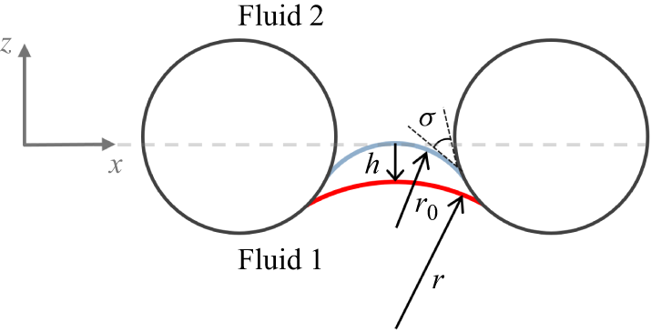
Illustration of a front separating two fluids. The interface in one of the pores (in red) is driven out of mechanical equilibrium with a small initial displacement
 $h(x,0)$
. Big circles represent the porous medium solid matrix.

2. Theory
2.1. Surface dynamic
Consider the interface between fluids 1 and 2, as shown in figure 1. Darcy’s law for two fluids in the absence of a gravitational field and neglecting inertia is given by
 \begin{equation} {{\boldsymbol {u}}_1}= -\frac {\kappa }{\mu _1} \boldsymbol{\nabla }\!{ \hat {P}_1}, \end{equation}
 \begin{equation} {{\boldsymbol {u}}_2}= -\frac {\kappa }{\mu _2} \boldsymbol{\nabla }\!{ \hat {P}_2}. \end{equation}
Here,
 ${\boldsymbol {u}}_{{i}}$
,
 $\hat {P}_i$
,
 $\mu _i$
are the Darcy velocity, pressure and viscosity of the phases
 $i=1,2$
, respectively, and
 $\kappa$
is the permeability. We decompose the pressure in each fluid into two components as
 \begin{equation} \hat {P}_i=P_i+p_i , \end{equation}
where
 $P_i$
denotes the constant background pressure in the fluid
 $i$
before or after any perturbation from mechanical equilibrium, and
 $p_i(x,z,t)$
represents the pressure perturbation induced by the disturbance. We define
 $z=0$
as the maximum interface height in the unperturbed pores (see figure 1).
We assume that the perturbations of the interface will be small compared to the characteristic pore size
 $a$
:
 \begin{equation} \lvert h(x,t) \rvert \ll a \;. \end{equation}
We further consider two incompressible fluids, which means that
 \begin{equation} \boldsymbol{\nabla }\boldsymbol{\cdot }{\boldsymbol {u}}_1=0, \quad \boldsymbol{\nabla }\boldsymbol{\cdot }{\boldsymbol {u}}_2=0, \end{equation}
and consequently, both fluids satisfy the Laplace equation for the pressure fields:
 \begin{equation} {\nabla} ^2p_1=0, \quad {\nabla} ^2p_2=0. \end{equation}
Taking the Fourier transform of the
 $x$
-coordinate in the above equations yields
 \begin{equation} \left(\frac {\partial ^2}{\partial z ^2}-q^2\right)p_i(q,z,t)=0, \end{equation}
where
 $i$
is
 $1$
or
 $2$
. The last equation is subject to the boundary condition that the pressure perturbations go to zero far away from the interface, which gives the solutions
 \begin{equation} p_1(q,z,t)=p_1(q,0,t)\,{\rm e}^{\lvert q \rvert z}, \end{equation}
 \begin{equation} p_2(q,z,t)=p_2(q,0,t)\,{\rm e}^{-\lvert q \rvert z}. \end{equation}
Consider a single pore as illustrated in figure 2, where the front moves from a position with radius of curvature
 $r_0$
, and touching
 $z=0$
, to one with radius of curvature
 $r=r_0+\Delta r$
, where
 $\Delta r \gt 0$
.
Illustration of a nonwetting fluid invading a wetting fluid at a single pore throat at different radii of curvature
 $r_0$
and
 $r=r_0+\Delta r$
. The distance moved between the two front positions is
 $h$
, and
 $\sigma$
is the wetting angle.

Let
 $z(r)$
denote the
 $ z$
-coordinates of the front with radius
 $r$
, and
 $z(r_0)$
the corresponding
 $ z$
-coordinates of the front with radius
 $ r_0$
. We then define
 $h$
as the extremum in
 $ z$
-deviation between the two curves. Note that in figure 2,
 $h$
is negative.
The distance
 $h$
to lowest order in
 $ \Delta r$
can be expressed as
 \begin{equation} h(x)= \left . \frac {\text{d}z}{\text{d}r} \right |_{r_0} \Delta r(x)= -\alpha \Delta r(x), \end{equation}
where
 \begin{equation} \alpha (\sigma ,p_{c0}) =- \left . \frac {\text{d}z}{\text{d}r} \right |_{r_0} \end{equation}
depends on the wetting angle
 $\sigma$
(see figure 2) and the capillary pressure
 $p_{c0}$
given by the Young–Laplace equation
 $p_{c0}=\gamma /r_0$
. We can then calculate the corresponding change in capillary pressure as
 \begin{equation} \Delta p_c=-\frac {\gamma \Delta r}{r_0^2}. \end{equation}
Then by using (2.10) and (2.12) we get
 \begin{equation} \Delta p_c = \frac {\gamma }{r_0^2 \alpha } h. \end{equation}
The capillary pressure at the interface can be written as
 \begin{align} p_c(x,t)&=p_1(x,h(x,t),t)-p_2(x,h(x,t),t))+p_{c0}\nonumber \\ &\approx p_1(x,0,t)-p_2(x,0,t)\nonumber \\ &\quad {}+\left(\frac {\partial p_1}{\partial z}\Bigg\vert _{z=0} - \frac {\partial p_2}{\partial z}\Bigg\vert _{z=0}\right) h(x,t)+p_{c0}, \end{align}
where
 $p_{c0}=P_1-P_2$
. Because the pressure difference
 $\partial p_i$
arises from the capillary pressure difference between the perturbed and unperturbed regions of the interface, we estimate
 $\partial p_i/\partial z$
as
 \begin{equation} \frac {\partial p_i}{\partial z} \sim \frac {\Delta p_c}{a}=\frac {{\gamma h}}{r_0^2 \alpha a}, \end{equation}
which is the maximum possible value for
 $\partial p_i/\partial z$
. This means that we can neglect the
 $\partial p_i/\partial z$
term in (2.14) to first order in
 $h$
, and get
 \begin{equation} p_c(x,t) \approx p_1(x,0,t)-p_2(x,0,t)+p_{c0} = \Delta p_c+p_{c0}=\varGamma h(x,t)+ p_{c0}, \end{equation}
where
 \begin{equation} \varGamma =\frac {\gamma }{r_0^2 \alpha }. \end{equation}
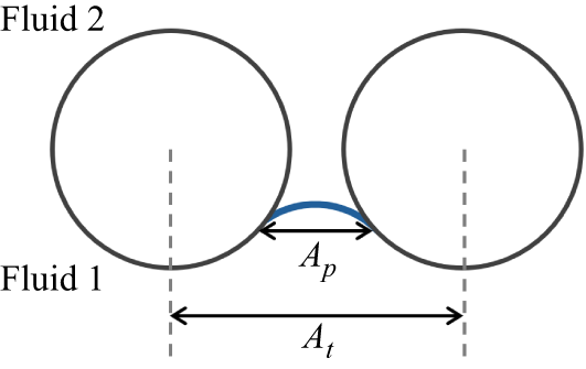
Illustration of the area corresponding to the cross-section of the pore neck where the fluid interface is located,
 $A_p$
, and the area
 $A_t$
including the solid part.

The
 $z$
-components of (2.1) and (2.2) at the interface are given by
 \begin{equation} \phi (h)\, \dot {h}=-\frac {\kappa }{\mu _i}\frac {\partial p_i}{\partial z}. \end{equation}
Here,
 $\phi (h)=A_p(h)/A_t$
, where
 $A_p(h)$
is the area corresponding to the cross-section of the pore neck at the position where the fluid interface is located, and
 $A_t$
is the area also including the solid part (see figure 3). We can now expand
 $\phi (h)$
and
 $\partial p_i/\partial z$
to first order in
 $h$
around
 $z=0$
, the position where
 $r=r_0$
. This gives
 \begin{equation} \frac {\partial p_i}{\partial z}= \frac {\partial p_i}{\partial z}\Bigg\rvert _{z=0}+\frac {\partial ^2p_i} {\partial z^2}\Bigg\rvert _{z=0} h \end{equation}
and
 \begin{equation} \phi (h)=\phi (0)+\frac {\partial \phi (z)}{\partial z} \Bigg\rvert _{z=0} h. \end{equation}
Since the fluid velocities are driven by the capillary pressure
 $\varGamma h$
, estimates for
 $\lvert \dot {h} \rvert$
and
 ${\partial ^2p_i}/{\partial z^2}$
may therefore be obtained as
 \begin{equation} \lvert \dot {h} \rvert \sim \frac {\kappa \varGamma h }{\mu _i a} \end{equation}
and
 \begin{equation} \frac {\partial ^2p_i}{\partial z^2} \sim \frac {\varGamma h}{a^2}. \end{equation}
As this is the maximum possible value for
 ${\partial ^2p_i}/{\partial z^2}$
, to first order in perturbation
 $h$
we get
 \begin{equation} \phi (0)\, \dot {h}=-\frac {\kappa }{\mu _i}\frac {\partial p_i}{\partial z} \Bigg\rvert _{z=0}. \end{equation}
The Fourier transforms of this equation using (2.8) and (2.9) then give
 \begin{equation} -\lvert q \rvert\, p_1(q,0,t)= \frac {\mu _1\, \phi (0)}{\kappa }\dot {h}(q,t), \end{equation}
 \begin{equation} \lvert q \rvert\, p_2(q,0,t)=\frac {\mu _2\, \phi (0)}{\kappa } \dot {h}(q,t). \end{equation}
We define the resistance terms
 $R_1$
and
 $R_2$
as
 \begin{equation} R_1=\frac {\mu _1\, \phi (0)}{\kappa }, \quad R_2=\frac {\mu _2\, \phi (0)} {\kappa }. \end{equation}
Adding (2.24) and (2.25) yields
 \begin{equation} \lvert q \rvert\, (p_1(q,0,t)-p_2(q,0,t))=-2 R\dot {h}(q,t), \end{equation}
where
 $R$
is defined as
 \begin{equation} R=(R_1+R_2)/2. \end{equation}
The Fourier transform of (2.16) gives
 \begin{equation} p_1(q,0,t)-p_2(q,0,t)= \varGamma h(q,t). \end{equation}
By inserting (2.29) into (2.27), we get
 \begin{equation} 2 R \dot {h}(q,t)+ \lvert q \rvert \varGamma h(q,t)=0, \end{equation}
which can be written as
 \begin{equation} \dot {h}(q,t)+\frac { \lvert q \rvert \varGamma }{2R} h(q,t)=0. \end{equation}
We assume an initial condition of the interface where one of the pores is brought out of equilibrium at the position
 $x=0$
with a small backward movement
 $h(x,0)=-\Delta A \delta (x)$
, where
 $\Delta A \phi (0)$
corresponds to a small area change in the fluid due to this movement. The fact that
 $h(x,0)$
diverges at
 $x=0$
implies that the resulting solution cannot be physically valid for the pore located at
 $x=0$
at very early times. The continuum Darcy description becomes meaningful only once the perturbation has propagated across multiple pores; otherwise, the assumptions underlying the continuum approximation break down. The Fourier transform of
 $h(x,0)$
is
 $h(q,0)=-\Delta A$
. With this, the solution to the first-order differential equation (2.31) is given by
 \begin{equation} h(q,t) = h(q,0)\,{\rm e}^{-\frac{\lvert q \rvert\, \varGamma t}{2R}} =- \Delta A{\rm e}^{-\frac{\lvert q \rvert\, \varGamma t}{2R}}. \end{equation}
This is followed by a final Fourier transform, which gives
 \begin{equation} h(x,t) = -\frac {\Delta A}{2 \pi } \int _{-\infty }^{\infty }{\rm e}^{-{\rm i}qx-\frac{\vert q \vert\, \varGamma t}{2R} }\, \text{d}q. \end{equation}
We can further perform the integral, which gives the surface displacement
 \begin{equation} h(x,t) = - \frac {\Delta A}{\pi } \times\frac { \frac{\varGamma t}{2R}}{\left(\frac{\varGamma t}{2R}\right)^2+x^2}. \end{equation}
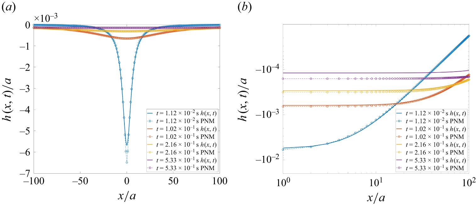
The surface displacement as a function of position is shown in figure 4 for different time values. The initial displacement was chosen as
 $h(x,0)=-\Delta A \delta (x)=-0.10\,a^2 \delta (x)$
, where
 $a$
is a characteristic pore size.
Normalised surface displacement
 $h(x,t)/a$
as a function of normalised pore position
 $x/a$
for different times
 $t$
(2-D case). The initial displacement was chosen as
 $h(x,0)=-\Delta A \delta (x)=-0.1\, a^2\!\delta (x)$
, and
 $v={\varGamma }/({2 R})=0.5$
m s−1. Continuous lines indicate results obtained with (2.34), while dashed lines with circles indicate numerical results, detailed in § 3. The same results are plotted in (a) linear scale and (b) logarithmic scale, for positive values of
 $x$
.

The minimum of
 $h(x,t)$
, denoted
 $h_{m}(x,t)$
, at a given position
 $x$
can be obtained by solving
 $\partial h(x,t)/\partial t=0$
, which yields
 \begin{equation} h_{m}(x,t_m) = - \frac {\Delta A}{2\pi x}, \end{equation}
where
 $t_m$
is the time at the minimum:
 \begin{equation} t_m=\frac {\lvert x \rvert\, 2R}{\varGamma }. \end{equation}
Hence the location
 $x$
at which
 $h(x,t)$
reaches its minimum with respect to time,
 $h_m(x,t_m)=- {\Delta A}/({2\pi x})$
, propagates with speed
 ${\varGamma }/({2R})$
. By introducing the scaled time
 $t/t_m$
and scaled height
 $h(x,t)/h_m(x,t_m)$
, we obtain a scaling function
 $g(t/t_m)$
that depends only on the dimensionless time
 $t/t_m(x)$
:
 \begin{equation} g(t/t_m)=\frac {h(x,t)}{h_m(x,t_m)}=\frac {2\frac{ \varGamma t}{2R\, \lvert x \rvert }}{\left(\frac{\varGamma t}{2Rx}\right)^2+1}=\frac { 2 \frac{t}{t_m}}{\left(\frac{t}{t_m}\right)^2+1}. \end{equation}
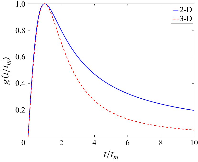
The scaling function
 $g(t/t_m)$
is shown for both the 2-D and 3-D cases in figure 5 (the 3-D case is calculated below), and shows a faster decay for large
 $t/t_m$
in three dimensions than in two dimensions. The maximum occurs at
 $t/t_m=1$
and has the value
 $g(1)=1$
as expected.
Since we describe the case where the total withdrawal rate of the fluids is zero, the total area of each of the two fluids must be conserved when integrated over the entire domain. Performing the integral gives
 \begin{equation} \phi (0)\int _{-\infty }^{\infty }h(x,t)\, \text{d}x=-\phi (0)\,\Delta A, \end{equation}
which confirms the conservation of area. Here, we have used the well-known result
 \begin{equation} \int _{-\infty }^{\infty } \frac {a}{a^2+x^2}\,\text{d}x=\pi. \end{equation}
Equation (2.34) has two simple asymptotic behaviours, at small and large times: with
 $v={\varGamma }/({2 R})$
,
 \begin{equation} h(x,t) \sim - \frac {\Delta A}{\pi vt} \end{equation}
at long times
 $t\gg x/v$
, and
 \begin{equation} h(x,t) \sim -\frac {\Delta A vt}{\pi x^2} \end{equation}
at short times
 $t\ll x/v$
(see figure 6).
The scaling function
 $g(t/t_m)$
as a function of the scaled time
 $t/t_m$
for the 2-D (solid line), and 3-D (stippled line) cases.

Normalised surface displacement
 $h(x,t)/a$
as a function of time
 $t$
(in seconds) for the 2-D case. The initial displacement was chosen as
 $h(x,0)=-\Delta A \delta (x) =-0.1\, a^2 \delta (x)$
, and
 $v={\varGamma }/({2 R})=0.5$
m s−1.

We note that when one of the fluids is much more viscous than the other (i.e. when
 $R_1$
or
 $R_2$
dominates),
 \begin{equation} v=\frac {\varGamma }{2 R} \approx \frac {\gamma \kappa }{\mu r_0^2 \alpha }, \end{equation}
where
 $\mu$
is the viscosity of the most viscous fluid, and
 $\kappa$
is the permeability of the medium.
Under these conditions, we can consider a quasi-2-D porous medium containing a front between air and water, with characteristic pore size
 $a$
, and thickness equivalent to 1 mm. Adopting
 $\kappa \sim 10^{-8} \,\text{m}^2$
(based on the permeability of a capillary tube with diameter
 $a=1$
mm),
 $\gamma =0.072\, \text{N}\,\text{m}^{-1}$
,
 $\mu \sim 10^{-3} \,\text{Pa}\,\,\text{s}$
and
 $r_0 \approx a/2$
, the speed
 $v={\gamma \kappa }/({\mu r_0^2 \alpha })$
is approximately
 $v \sim 3 \,\text{m}\,\text{s}^{-1} \times({1}/{\alpha })$
, which might be of the order of
 $\text{m}\ \text{s}^{-1}$
depending on the geometric constant
 $ \alpha$
.
We can generalise our results to 3-D porous media idealised as pores connected by converging–diverging cylindrical tubes. In this case, the meniscus inside each tube at the front would have two identical principal radii of curvature that vary according to (2.10). In this system, the equilibrium capillary pressure would be given by
 $p_{c0}=2\gamma /r_0$
, leading to
 $ \varGamma ={2\gamma }/{r_0^2 \alpha }$
. This corresponds to the expression in (2.17) simply multiplied by a factor 2. Departing from this small correction, to generalise the situation to three dimensions with a 2-D front (instead of a one-dimensional line), we perform a 2-D Fourier transform of
 \begin{equation} h(x,y,0))=-\Delta V \delta (x) \delta (y) \end{equation}
to find
 $h(q_x,q_y,0)=-\Delta V$
. We further replace
 $\text{d}q$
with
 $\text{d}q^2$
in (2.33), and perform a 2-D Fourier transform. Here,
 $q=(q_x^2+q_y^2)^{1/2}$
and
 $\boldsymbol {q}=(q_x,q_y)$
. The Fourier transform of
 $h(\boldsymbol {q},t)$
can then be expressed in polar coordinates as
 \begin{align} h(r,t)=-\frac {\Delta V }{(2 \pi )^2} \int _{\boldsymbol {q}} {\rm e}^{-{\rm i}{\boldsymbol {q} \boldsymbol{\cdot }\boldsymbol {r}}-\frac{q \varGamma t}{2R}}\, \text{d}^2q =-\frac {\Delta V}{(2 \pi )^2} \int _0^{\infty } \int _0^{2 \pi } {\rm e}^{{\rm i}r q \cos{\theta }-\frac{q \varGamma t}{2R}}q \,\text{d}\theta\, \text{d}q, \end{align}
where
 $\boldsymbol {r}=(x,y)$
is the position vector from the centre of the perturbed pore,
 $r=(x^2+y^2)^{1/2}$
, and
 $\theta$
is the angle between
 $\boldsymbol {r}$
and
 $\boldsymbol {q}$
. Using the identity for the zeroth-order Bessel function of the first kind
 \begin{equation} J_0(rq)=\frac {1}{2 \pi }\int _0^{2 \pi }{\rm e}^{{\rm i}r q\kern-1pt\cos{\theta }}\, \text{d} \theta, \end{equation}
we obtain
 \begin{equation} h(r,t)= -\frac {\Delta V}{2 \pi } \int _0^{\infty } J_0(rq)\,{\rm e}^{-\frac{q \varGamma t}{2R}}\, q\text{d}q. \end{equation}
This expression can be further rewritten as
 \begin{align} h(r,t)=\frac {\Delta \textit{VR}}{ \pi \varGamma } \frac {\partial }{\partial t} \int _0^{\infty } J_0(rq)\,{\rm e}^{-\frac{q \varGamma t}{2R}}\, \text{d}q = \frac {\Delta \textit{VR}}{ \pi \varGamma } \frac {\partial }{\partial t} \int _0^{\infty } J_0(rq)\,{\rm e}^{-q\,{\hat s}(t)}\, \text{d}q, \end{align}
where
 ${\hat s}=\varGamma t/(2R)$
. Equation (2.47) represents the time derivative of the Laplace transform of the zeroth-order Bessel function
 $J_0(rq)$
, where
 ${\hat s} = \varGamma t/(2R)$
. This Laplace transform has the well-known solution
 $({\hat s}^2+r^2)^{-1/2}$
, which yields
 \begin{equation} h(r,t)=\frac {\Delta \textit{VR}}{ \pi \varGamma }\frac {\partial }{\partial t} \frac {1}{({\hat s}^2+r^2)^{1/2}} = -\frac {\Delta V }{2 \pi } \frac {\frac{\varGamma t}{2R}}{\left(r^2+\left(\frac{\varGamma t}{2R}\right)^2\right)^{3/2} }. \end{equation}
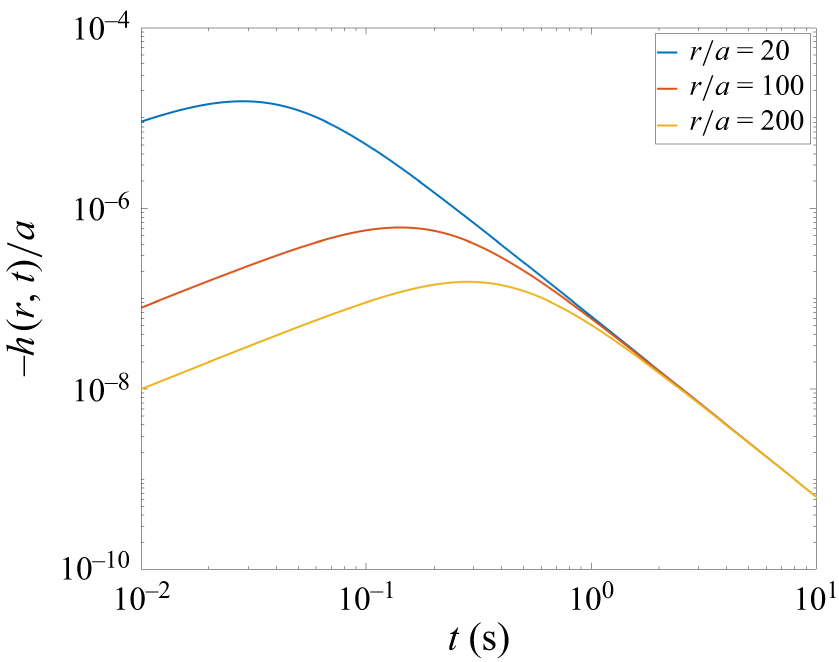
Normalised surface displacement
 $h(r,t)/a$
as a function of time
 $t$
(in seconds) for the 3-D case. The initial displacement was chosen as
 $h(x,y,0)=-\Delta V \delta (x) \delta (y)=-0.1\, a^3 \delta (x) \delta (y)$
, and
 $v={\varGamma }/({2 R})= 0.5$
m s−1.

This solution has a faster decay of the interface perturbation in space and time compared to the 2-D case.
In this calculation, the gravitational field was neglected – an approximation that is good if
 $\varGamma \gg \lvert \Delta \rho \rvert\, g$
, where
 $\Delta \rho$
is the density difference between the two fluids, and
 $g$
is the acceleration due to gravity.
Equation (2.48) exhibits two distinct asymptotic behaviours in the limits of small and large times:
 \begin{equation} h(r,t) \sim - \frac {\Delta V}{2\pi (vt)^2} \end{equation}
at long times
 $t\gg x/v$
, and
 \begin{equation} h(r,t) \sim -\frac {\Delta V vt}{2 \pi r^3} \end{equation}
at short times
 $t\ll x/v$
(see figure 7). Figure 8 shows the surface displacement as a function of distance at different times.
Normalised surface displacement
 $h(r,t)/a$
as a function of normalised pore position
 $r/a$
for different times
 $t$
for the 3-D case. The initial displacement was chosen as
 $h(x,y,0)=-\Delta V \delta (x) \delta (y)=-0.1\, a^3 \delta (x) \delta (y)$
, and
 $v={\varGamma }/({2 R})=0.5$
m s−1.

The minimum of
 $h(r,t)$
, denoted
 $h_{m}(r,t)$
, at a given position
 $r$
can again be obtained by
 $\partial h(r,t)/\partial t=0$
, which yields
 \begin{equation} h_{m}(r,t_m) = - \frac {\Delta V}{\pi 3^{3/2} r^2}, \end{equation}
where
 \begin{equation} t_m= \frac {r 2^{1/2}R}{ \varGamma } \end{equation}
is the time at which the minimum occurs. Hence the location
 $r$
at which
 $h(r,t)$
reaches its minimum
 $h_m(r,t_m)=- {\Delta V}/({\pi 3^{3/2} r^2})$
propagates with speed
 ${\varGamma }/{(2^{1/2} R)}$
. By introducing the scaled time
 $t/t_m$
and scaled height
 $h(r,t)/h_m(r,t_m)$
, we obtain, similarly to the 2-D case, a scaling function
 $g(t/t_m)$
that depends only on the dimensionless time
 $t/t_m(x)$
:
 \begin{equation} g(t/t_m)=\frac {h(r,t)}{h_m(r,t_m)}=\frac {\frac{t}{t_m} \left(\frac {3}{2}\right)^{3/2}}{\left(1+\frac {1}{2} \left(\frac{t}{t_m}\right)^2\right)^{3/2}}. \end{equation}
The scaling function
 $g(t/t_m)$
is shown for both the 2-D and 3-D cases in figure 5.
Since the solution describes the case where the withdrawal rate is zero, the total volume of each of the two fluids must be conserved. Performing the integral
 \begin{equation} \phi (0)\int _0^{\infty }\int _0^{2\pi }h(r,t)\,r \,\text{d}r\, \text{d}\theta =-\phi (0)\,\Delta V \end{equation}
confirms the volume conservation. Here, we have used the integral
 \begin{equation} \int _0^{\infty } \frac {ax}{(x^2+a^2)^{3/2}}\,\text{d}x=1. \end{equation}
2.2. Characteristic time and length scales for the Haines jump
We now consider the case where the interface is also moving due to an external flow. Since the location
 $x$
corresponding to the minimum of
 $h(x,t)$
propagates with speed
 $v \propto {\varGamma }/{R}$
in two and three dimensions, a characteristic time for the Haines jump is given by
 $t_h=L/v$
, where
 $L$
is the size of the system. Another characteristic time scale is
 $t_e=a/v_e$
, which corresponds to the time required for the interface to advance by one pore length
 $a$
due to the external flow rate
 $q=S v_e$
, where
 $S$
is the cross-section of the model, and
 $v_e$
is the Darcy velocity. The ratio between these two time scales is given by
 \begin{equation} \frac {t_h}{t_e}=\frac {v_e \mu }{\gamma } \frac {L}{a}\left(\frac {r_0^2 \alpha }{\kappa }\right)\!, \end{equation}
using (2.17). Equation (2.56) can be interpreted as a modified capillary number expressing the ratio between the viscous pressure drop over the characteristic length scale of the model and the capillary pressure. When the modified capillary number is large,
 ${t_h}/{t_e}\gg 1$
, the displacement is dominated by viscous forces; in contrast, when
 ${t_h}/{t_e}\ll 1$
, capillary forces dominate (Lenormand et al. Reference Lenormand, Touboul and Zarcone1988; Méheust et al. Reference Méheust, Løvoll, Måløy and Schmittbuhl2002). Under the assumption that the last term within the parentheses is of order one, this is consistent with the estimate made by Furuberg et al. (Reference Furuberg, Måløy and Feder1996). When the ratio
 $t_h/t_e\lt 1$
is satisfied, the flow will be controlled by the dynamics of the Haines jumps. However, when
 $t_h/t_e\gt 1$
, the Darcy velocity dominates the flow, but only above a characteristic length scale
 $\eta$
, which is determined by solving
 \begin{equation} \frac {v_e \mu }{\gamma } \frac {\eta }{a}\left(\frac {r_0^2 \alpha }{\kappa }\right)=1, \end{equation}
giving
 \begin{equation} \eta =\frac {\gamma \kappa a}{v_e \mu r_0^2 \alpha } \;. \end{equation}
Below this length scale, the dynamics will be controlled by the Haines jump dynamics.
2.3. Pressure and velocity field
For simplicity, we now consider the case in which fluid 1 is a gas, and its pressure is assumed constant,
 $\hat {P}_1=P_1$
. We begin by examining the 2-D configuration. Once the surface displacement
 $h(q,t)$
of the interface is known, the pressure field
 $p_2(q,z)$
can be determined by using (2.9), (2.29) and (2.32), which yields
 \begin{equation} p_2(q,z,t)=-\varGamma h(q,t)\,{\rm e}^{-\lvert q \rvert\, z}= \varGamma \Delta A {\rm e}^{-\frac{\lvert q \rvert\, \varGamma t}{2R}}\,{\rm e}^{-\lvert q \rvert \,z}. \end{equation}
Then, by an inverse Fourier transform, we get
 \begin{align} p_2(x,z,t)= \frac {\varGamma \Delta A}{2 \pi } \int _{-\infty }^{\infty } {\rm e}^{-{\rm i}qx-\frac{\vert q \vert\, \varGamma t}{2R}-\vert q \vert\, z}\, \text{d}q = \frac {\varGamma \Delta A}{\pi } \times \frac { \left(\frac{\varGamma t}{2R}+z \right)}{\left(\frac{\varGamma t}{2R}+z\right)^2+x^2}. \end{align}
An example of a theoretical pressure field obtained with (2.60), at time
 $t=1.22\times 10^{-3}$
s, is shown in figure 10(a) below. The initial displacement was chosen as
 $h(x,0)=-\Delta A \delta (x)=-0.1\, a^2 \delta (x)$
, and
 $v={\varGamma }/({2 R})=0.5$
m s−1. A contour plot of the scaled pressure field is also shown in figure 9(a), for any
 $t\gt 0$
. Since the velocity is proportional to
 $- \boldsymbol{\nabla }p_2$
, the slope of the contours at
 $z=0$
shows that the front is first back-contracting for
 $|x| \gt \varGamma t/(2R)$
, and advancing again at later times when
 $|x| \lt \varGamma t/(2R)$
. Moreover, as the
 $z$
-dependence of
 $p_2$
in (2.60) is only via the compound
 $z+\varGamma t/(2R)$
, the pressure map moves at constant speed
 $-\varGamma /(2R)$
along the
 $z$
-axis, perpendicular to the interface. This can be seen in a movie of
 $p_2$
at different times, included in the supplementary material is available at https://doi.org/10.1017/jfm.2026.11960.
Contour plot of the scaled pressure perturbation in fluid 2,
 $p_2$
, for any
 $t\gt 0$
, for the (a) 2-D and (b) 3-D cases. In (a), for
 $|x| \gt \varGamma t/(2R)$
, the front back-contracts, as indicated by the slope of the contours at
 $z=0$
. Similarly, in (b), the front back-contracts for
 $|r| \gt \varGamma t/(\sqrt 2\, R)$
.

Values of (a)
 $p_2$
, (d) magnitude of
 $u_{2x}$
and (g) magnitude of
 $u_{2z}$
, given by (2.60)–(2.62), respectively. In this example, the initial displacement was chosen as
 $h(x,0)=-\Delta A \delta (x)=-0.1\, a^2 \delta (x)$
, and
 $v={\varGamma }/({2 R})=0.5$
m s−1. The pressure and velocity fields were generated at
 $t=1.22\times 10^{-3}$
. (b,e,h) Similar results, obtained with the PNM described in § 3. (c, f,i) A comparison between theoretical and numerical results. A window of
 $201a\times 201a$
pores is shown.

With the expression for the pressure field in fluid 2 established, we can now compute the Darcy velocity field using (2.2):
 \begin{equation} u_{2x}=-\frac {\kappa }{\mu _2} \frac {\partial p_2(x,z,t)}{\partial x}= \frac {\kappa }{\mu _2}\frac {\varGamma \Delta A}{\pi }\times\frac {\big(\frac{\varGamma t}{2R}+z\big)2x}{\Big(\big(\frac{\varGamma t}{2R}+z\big)^2+x^2\Big)^2}, \end{equation}
 \begin{equation} u_{2z}=-\frac {\kappa }{\mu _2} \frac {\partial p_2(x,z,t)}{\partial z} =\frac {\kappa }{\mu _2} \frac {\varGamma \Delta A}{\pi }\times\frac {\big(\frac{\varGamma t}{2R}+z\big)^2-x^2}{\Big(\big(\frac{\varGamma t}{2R}+z\big)^2+x^2\Big)^2}. \end{equation}
The calculated velocity fields at time
 $t=1.22\times 10^{-3}$
s are shown in figures 10(d) and 10(g), with the same initial values
 $h(x,0)$
and
 $v$
as for the pressure field in figure 10(a). We can observe in these results that the predicted flow velocities reach the order of cm s−1 at early times. With characteristic pore size 1 mm, and considering an interface between air and water, this suggests that in the vicinity of the originally out-of-equilibrium meniscus, inertial effects might be relevant and should be further evaluated. However, (2.61) and (2.62) also indicate that these high velocities rapidly decay with time and do not reach distances beyond two pores away from the jump origin.
When extended to three dimensions, the calculation proceeds analogously, and gives
 \begin{align} p_2(r,t)&= \frac {\varGamma \Delta V }{(2 \pi )^2} \int _{\boldsymbol {q}} {\rm e}^{-{\rm i}{\boldsymbol {q} \boldsymbol{\cdot }\boldsymbol {r}}-\frac{q \varGamma t}{2R}-qz}\, \text{d}^2q\nonumber \\ &=\frac {\varGamma \Delta V}{(2 \pi )^2} \int _0^{\infty } \int _0^{2 \pi } {\rm e}^{{\rm i}r q\kern-1pt \cos{\theta }-\frac{q \varGamma t}{2R}-qz} q \text{d}\theta \text{d}q \nonumber \\ &= \frac { \varGamma \Delta V }{2 \pi } \frac {\left(\frac{\varGamma t}{2R}+z\right)}{\left(r^2+\left(\frac{\varGamma t}{2R}+z\right)^2\right)^{3/2} } \end{align}
for the pressure
 $p_2(r,t)$
. A contour plot of the scaled pressure field is shown in figure 9(b), for any
 $t\gt 0$
. The slope of the contours at
 $z=0$
shows that the front is first back-contracting for
 $|r| \gt \varGamma t/(\sqrt {2}\,R)$
, and advancing again at later times when
 $|r| \lt \varGamma t/(\sqrt {2}\,R)$
. With this expression for the pressure, we can calculate the Darcy velocity field using (2.2):
 \begin{equation} u_{2x}=-\frac {\kappa }{\mu _2} \frac {\partial p_2(x,y,z,t)}{\partial x} =\frac {\kappa \varGamma \Delta V}{\mu _2 2 \pi } \times\frac {3\big( \frac{\varGamma t}{2R}+z\big)x}{\Big(x^2+y^2+\big(\frac{\varGamma t}{2R}+z\big)^2\Big)^{5/2}}, \end{equation}
 \begin{equation} u_{2y}=-\frac {\kappa }{\mu _2} \frac {\partial p_2(x,y,z,t)}{\partial y} =\frac {\kappa \varGamma \Delta V}{\mu _2 2 \pi } \times\frac {3\big(\frac{\varGamma t}{2R}+z\big)y}{\Big(x^2+y^2+\big(\frac{\varGamma t}{2R}+z\big)^2\Big)^{5/2}}, \end{equation}
 \begin{equation} u_{2z}=-\frac {\kappa }{\mu _2} \frac {\partial p_2(x,y,z,t)}{\partial z} =\frac {\kappa \varGamma \Delta V}{\mu _2 2 \pi } \times\frac {2\big(\frac{\varGamma t}{2R}+z\big)^2-x^2-y^2}{\Big(x^2+y^2+\big(\frac{\varGamma t}{2R}+z\big)^2\Big)^{5/2}}. \end{equation}
2.4. Including the gravitational field
So far, we have neglected the gravitational field. Including the gravitational field
 $-{{\boldsymbol {e}}_{{z}}}\,g$
, where
 ${\boldsymbol {e}}_{{z}}$
is a unit vector in the
 $z$
-direction, Darcy’s law for two fluids can be written as
 \begin{equation} {{\boldsymbol {u}}_{{i}}}= -\frac {\kappa }{\mu _i} \boldsymbol{\nabla }({ \hat {P}_i} +\rho _i g z), \end{equation}
where
 $\rho _i$
is the density of fluid
 $i$
. We then introduce the potential function
 ${\hat \varPsi _i}={\hat P_i}+\rho g z$
. In a manner analogous to the pressure, the potential function
 ${\hat \varPsi }_i$
in each fluid can be decomposed into two components as
 \begin{equation} {\hat \varPsi _i}=\varPsi _i+\psi _i , \end{equation}
where
 $\varPsi _i$
denotes the constant background potential in the fluid
 $i$
prior to any perturbation from mechanical equilibrium, and
 $\psi _i(x,z,t)$
represents the perturbation of the potential induced by the disturbance and plays the role of
 $p_i(x,z,t)$
in the calculation without a gravitational field. The boundary condition at the interface will then be given by
 \begin{align} p_c(x,t)+\Delta \rho g h(x,t) &\approx \psi _1(x,0)-\psi _2(x,0)+p_{c0} \nonumber \\ &=\Delta p_c+p_{c0}+\Delta \rho\, g\, h(x,t)\nonumber \\ &=\varGamma h(x,t) + \Delta \rho\, g\, h(x,t) + p_{c0}, \end{align}
where
 $\Delta \rho =\rho _1-\rho _2$
. Then if we define
 \begin{equation} {\hat \varGamma }=\varGamma +\Delta \rho\, g, \end{equation}
the corresponding equations in the presence of a gravitational field are identical to those derived above without a gravitational field, provided that
 $\varGamma$
is replaced by
 $\hat \varGamma$
. It is important to note that negative values of
 $\hat \varGamma$
would result in an unstable configuration not leading to the front back-contraction described by the proposed model.
3. Numerical modelling
In this section, the proposed theoretical model for interface displacement subjected to a localised, transient perturbation in a 2-D porous medium is compared to numerical results obtained with a PNM. For this, we adapt the dynamic PNM proposed by Reis et al. (Reference Reis, Linga, Moura, Rikvold, Toussaint, Flekkøy and Måløy2025) to represent the drainage of a liquid by an inviscid and weightless gas. This model incorporates the effects of capillary and viscous forces on the wetting phase, while considering a constant pressure within the non-wetting phase. In addition, it uses a fully implicit method to solve equations relating the pressure in the pores and the meniscus position in the pore throats, making it suitable to represent low-capillary-number porous media flows. The simulation parameters and required PNM adaptations are presented next. For more details regarding the model, refer to Reis et al. (Reference Reis, Linga, Moura, Rikvold, Toussaint, Flekkøy and Måløy2025).
3.1. Pore-network and fluid properties
In a PNM, porous media are represented as networks of pores (sites) connected by pore throats (bonds). For the sake of simplicity, a square lattice is adopted here as the pore network. To make the numerical results comparable to the theoretical model presented in § 2, a large domain of
 $801\times 200$
pores is simulated. As the adopted model represents the fluid flow only within the viscous wetting phase, this domain encompasses the interface between the fluids and the region of the porous medium occupied by fluid 2.
The pore-throat length used in the PNM simulations is
 $a=1$
mm, and the in-plane radius at the meniscus initial equilibrium position is
 $r_0=0.5$
mm. The flow within each pore throat is approximated as a Poiseuille flow in a cylindrical tube of length and diameter equivalent to
 $1$
mm, while the volume and the viscous pressure drop in the pores are considered negligible. With this, the pore-network permeability is equivalent to
 $\kappa =2.45\times 10^{-8}$
m
 $^2$
, computed with a single-phase flow simulation and Darcy’s law.
The viscosity of water is assigned to fluid 2, i.e.
 $\mu _2=1\times 10^{-3}$
Pa s, and the interfacial tension between water and air,
 $\gamma =72\times 10^{-3}$
N m−1, is used to calculate the capillary pressure. Using
 $\mu _2$
,
 $k$
and negligible
 $\mu _1$
, the resistance parameter, defined in (2.28), is
 $R=2.04\times 10^{4}$
Pa s m
 $^{-2}$
. To match the conditions used to obtain the theoretical results shown in figure 4, where
 $v={\gamma }/{(2Rr_0^2\alpha)}=0.5$
m s−1, value
 $\alpha =14.13$
is adopted. With these parameters, the variation in capillary pressure with
 $h$
proposed in (2.16) can be implemented in the PNM.
3.2. Initial and boundary conditions
In the initial fluid configuration, the interface is located adjacent to the bottom boundary of the
 $801\times 200$
pore network. To represent this, the pores at
 $z=0$
are occupied by the non-wetting phase, while all other pores are occupied by the wetting phase. Pore throats between pores occupied by different phases contain the interface menisci, which can be moved from
 $-a/2$
to
 $a/2$
along the throat. To create an unstable interface configuration similar to the illustration in figure 1, the meniscus of the central pore throat (at
 $x=0$
) is located at
 $h(0,0)=-a/10$
, while
 $h(x\neq 0,0)=0$
. A simple sketch of the pore network and initial fluid configuration is presented in figure 11.
From the initial mechanically unstable state, fluid is redistributed along the interface until a new equilibrium position is found, when all menisci have the same displacement
 $h$
, and the capillary pressure along the interface is constant. During the fluid redistribution, the pore-network boundaries at
 $x=-400a$
,
 $x=400a$
and
 $z=200a$
are closed to the flow.
Sketch of the pore network and initial fluid configuration. Circles represent the network pores (sites), and rectangles represent the network pore throats (bonds), forming a square lattice. Blue indicates network elements initially occupied by the wetting phase, and white indicates elements occupied by the non-wetting phase. Red arcs indicate where the menisci separating the fluids are initially located, with the central meniscus displaced with respect to the others, leading to an unstable configuration.

3.3. Results
In figure 4, the normalised surface displacements obtained with (2.34) and the PNM for different times are compared. We can notice that except for very low times and
 $x\approx 0$
, the numerical and theoretical solutions display excellent agreement. Since the theoretical model adopts
 $h(x,0)=-\Delta A \delta (x)$
as the initial condition, representing an initial displacement
 $\Delta A/a$
over a pore of length
 $a$
, we expected this small deviation to occur between the results. Another source of disagreement between numerical and theoretical results is related to the finite size of the pore network used in the PNM. As the interface reaches the mechanical equilibrium configuration, the excess wetting fluid initially contained in the central pore throat is equally distributed among all pore throats at the interface. For an infinite interface, each pore throat gets an infinitesimally small amount of fluid, leading to
 $h(x,t\rightarrow \infty )\approx 0$
. In finite systems, the smaller the interface, the larger the final displacement. The effect of this fluid redistribution in the numerical results can be seen in figure 4, at larger times. It also becomes clear in figure 12. In this plot, we compare the theoretical scaling function
 $g(t/t_m)$
for 2-D porous media, introduced in (2.37), with the equivalent PNM results, for different positions along the interface. For
 $t\leqslant t_m$
or small
 $x$
, the numerical results agree well with the scaling function. Far from the initial interface perturbation, however, the maximum meniscus displacement during the back-contraction becomes similar to the final displacement at the new mechanical equilibrium. To minimise this effect, larger pore networks could be used in our PNM simulations.
The scaling function
 $g(t/t_m)$
as a function of the scaled time
 $t/t_m$
for the 2-D case (solid line), compared with the results obtained with the PNM (dashed lines) for different positions along the interface.

The solutions for the pressure perturbation and velocity fields proposed in (2.60)–(2.62) are also reproduced with the PNM. For the
 $p_2$
results, the pressure perturbation in the pore-network sites filled with the wetting phase is represented in figure 10(b). The numerical velocity fields corresponding to
 $u_{2x}$
and
 $u_{2z}$
are presented in figures 10(e) and 10(h), respectively. Since a square lattice is adopted as the pore network, each pore throat has either velocity in the
 $x$
- or
 $z$
-direction. We explore this feature, and display in figure 10(e) only the velocity results related to the horizontal pore throats. Conversely, in figure 10(h), only the velocities in the vertical pore throats are shown.
A comparison between theoretical and numerical results is presented in figures 10(c), 10(f) and 10(i), indicating a good qualitative and quantitative consistency between pressure and velocity fields obtained with both methods. A progressive mismatch between solutions can be observed towards the tops of the images, which we attribute to boundary effects in the numerical solution. As the pore network contains only 200 pores in the
 $z$
-direction, the flow near this region can be affected by the imposed ‘no-flow’ boundary condition, which does not reflect the theoretical model. Figure 10(i) also displays a noticeable disagreement between
 $u_{2z}$
and
 $u_z^{PNM}$
near
 $x=0$
,
 $z=0$
, where the initially out-of-equilibrium meniscus is located. This discrepancy is likely related to the initial theoretical front profile
 $h(x,0)=-\Delta A \delta (x)$
, which affects the comparison between results in early times, as seen in figure 4.
Detailed representations of the velocity field obtained with the PNM are shown in figure 13, for different times. In these images, both vertical and horizontal pore throats are represented, and arrows indicate the flow direction. The front menisci are located at the bottom-most vertical pore throats, while all other pore throats are filled with fluid 2 (see figure 11). As discussed in § 2.3, the front back-contracts for
 $|x|\gt \varGamma t/(2R)$
and advances for
 $|x|\lt \varGamma t/(2R)$
. This theoretical prediction is verified in figures 13(a) and 13(b). In figure 13(a), at
 $t=1.22\times 10^{-3}$
s, we expect all menisci located at
 $|x|\gt 6.1\times 10^{-4}$
m to back-contract, given that
 $\varGamma /2R=0.5$
m s−1. For pore size
 $a=1\times 10^{-3}$
m, this means that all menisci, except the central one at
 $x=0$
, back-contract, as indicated by the downward-pointing arrows. In figure 13(b), at
 $t=7.69\times 10^{-3}$
s, this distance increases to
 $|x|\gt 3.84\times 10^{-3}$
m, and we can observe that the flow in all front pore throats located below this threshold points upwards, indicating the front advancement.
The PNM used in this work satisfactorily represents the dynamics of a Haines jump theoretically predicted in § 2. As such, it should also serve as a valuable numerical tool for analysing how these dynamics would change under broader drainage flow conditions. In the supplementary material, we provide additional numerical results using pore networks with variable pore sizes. Further extensions to the porous medium or flow parameters will be explored in future studies.
Detailed representations of the velocity profile in the square pore network. In each pore throat, an arrow indicates the direction of the flow. The bottom-most vertical pore throats in each image contain the front menisci separating fluids 1 and 2, as illustrated in figure 11. A window of
 $31 \times 31$
pores is shown.

4. Conclusion
We investigated a scenario in which a single pore is displaced from mechanical equilibrium along the interface between two fluids within a porous medium. Since there is no outflow from the system, a flow will develop between the initial perturbation and the surrounding interface. As a result, the interface will retract, creating a time- and space-dependent profile. For the sake of simplicity, we considered the interface to be flat. This condition can typically be achieved experimentally by utilising a pore throat distribution in which all pores are uniform in size, except for a localised region with larger pore throats, suggesting the need for new experiments that should be compared with the theoretical results.
Analytical solutions have been derived for cases where inertial effects can be neglected. We examined both the two-dimensional case, in which the fluid front is modelled as a flat line, and the three-dimensional case, in which the front is a flat surface. The two-dimensional solutions for the interface displacement, pressure and velocity fields were compared with numerical results from a pore-network model, showing good agreement.
Furthermore, our findings underscore the necessity to explore more general scenarios, particularly the influence of fractal interfaces on flow dynamics. This exploration is especially pertinent in the context of two-phase flow in porous media, where numerous practical applications arise, such as groundwater flow management and enhanced hydrocarbon recovery. Future research should focus on unravelling these complexities to enhance predictive models and facilitate better applications across various fields.
Supplementary material
Supplementary material is available at https://doi.org/10.1017/jfm.2026.11960.
Acknowledgements
The authors acknowledge M. Moura and M. Ayaz for useful discussions.
Funding
We thank for their the support the University of Oslo, the University of Strasbourg, CNRS, and IRP D-FRRACT, and the Research Council of Norway, through the PoreLab Centre of Excellence (project no. 262644).
Declaration of interests
The authors report no conflict of interest.
Data availability statement
The data that support the findings of this study can be made available upon request.
Author contributions
P.R.: methodology, software, validation, writing – original draft. E.G.F.: methodology, formal analysis, writing – review/editing. R.T.: methodology, formal analysis, writing – review/editing. K.J.M.: conceptualisation, methodology, formal analysis, investigation, writing – original draft, supervision, funding acquisition.

 h(x,0)
 r0
 r=r0+Δr
 h
 σ
 Ap
 At
 h(x,t)/a
 x/a
 t
 h(x,0)=−ΔAδ(x)=−0.1a2δ(x)
 v=Γ/(2R)=0.5
 x
 g(t/tm)
 t/tm

 h(x,t)/a
 t
 h(x,0)=−ΔAδ(x)=−0.1a2δ(x)
 v=Γ/(2R)=0.5
 h(r,t)/a
 t
 h(x,y,0)=−ΔVδ(x)δ(y)=−0.1a3δ(x)δ(y)
 v=Γ/(2R)=0.5

 h(r,t)/a
 r/a
 t
 h(x,y,0)=−ΔVδ(x)δ(y)=−0.1a3δ(x)δ(y)
 v=Γ/(2R)=0.5

 p2
 t>0
 |x|>Γt/(2R)
 z=0
 |r|>Γt/(2R)

 p2
 u2x
 u2z
 h(x,0)=−ΔAδ(x)=−0.1a2δ(x)
 v=Γ/(2R)=0.5
 t=1.22×10⁻³
 201a×201a


 g(t/tm)
 t/tm

 31×31


 Open access

