1. Introduction
The experimental discovery of transition to ‘elastoinertial turbulence’ (EIT) (Samanta et al. Reference Samanta, Dubief, Holzner, Schäfer, Morozov, Wagner and Hof2013; Choueiri, Lopez & Hof Reference Choueiri, Lopez and Hof2018; Chandra et al. Reference Chandra, Shankar and Das2018, Reference Chandra, Shankar and Das2020; Choueiri et al. Reference Choueiri, Lopez, Varshney, Sankar and Hof2021) in pipe flow of dilute-to-semidilute polymer solutions, at Reynolds numbers (
 $Re$
) much lower than the Newtonian threshold (
 $Re \approx 2000$
), has led to renewed interest in understanding the onset of turbulence in viscoelastic flows. In particular, recent efforts have shown that both viscoelastic pipe (Garg et al. Reference Garg, Chaudhary, Khalid, Shankar and Subramanian2018; Chaudhary et al. Reference Chaudhary, Garg, Subramanian and Shankar2021) and channel flows (Khalid et al. Reference Khalid, Chaudhary, Garg, Shankar and Subramanian2021a
) are susceptible to an elastoinertial ‘centre-mode’ instability, with the unstable centre modes having phase speeds close to the base-state maximum. There is some experimental evidence of EIT onset in pipe flow being triggered by the centre-mode instability (Chandra, Shankar & Das Reference Chandra, Shankar and Das2018; Choueiri et al. Reference Choueiri, Lopez, Varshney, Sankar and Hof2021), especially at relatively low elasticity numbers
 $E \lt 0.1$
(here,
 $E = W/Re$
, with
 $W$
being the Weissenberg number defined below). At higher
 $E$
values, while the flow is linearly stable within the Oldroyd-B paradigm, experiments nevertheless report a transition, presumably due to a subcritical mechanism (Choueiri et al. Reference Choueiri, Lopez, Varshney, Sankar and Hof2021). Indeed, recent efforts have used a weakly nonlinear framework to characterise the dominantly subcritical nature of bifurcation underlying the centre-mode instability (Wan, Sun & Zhang Reference Wan, Sun and Zhang2021; Buza, Page & Kerswell Reference Buza, Page and Kerswell2022; Dong & Zhang Reference Dong and Zhang2022). Even more recently, Kerswell & Page (Reference Kerswell and Page2024) have analysed the centre-mode instability using a matched asymptotic expansions approach, and predicted the unstable eigenvalue for both the elastoinertial (for
 $Re \gg 1$
) and elastic (for
 $E \gg 1$
, discussed below) cases.
Although the experimental studies quoted above have focused on pipe flows, there have been other studies, by Arratia and co-workers (Pan et al. Reference Pan, Morozov, Wagner and Arratia2013; Qin & Arratia Reference Qin and Arratia2017; Qin et al. Reference Qin, Salipante, Hudson and Arratia2019), which reported a transition to complex flow states, even at very low
 $Re$
, in viscoelastic pressure-driven flow through square channels, the transition likely triggered by finite-amplitude perturbations induced by tiny pillars at the channel inlet. Later, Steinberg and co-workers (Jha & Steinberg Reference Jha and Steinberg2020, Reference Jha and Steinberg2021) used rectangular channels with cross-sectional aspect ratio 7 : 1, closer to the theoretical plane Poiseuille scenario, and have shown that elastic coherent structures are again triggered by inlet pillars, akin to the set-up of Arratia and co-workers. In more recent experiments, Shnapp & Steinberg (Reference Shnapp and Steinberg2022) and Li & Steinberg (Reference Li and Steinberg2022) report instabilities in a rectangular channel flow even in the absence of inlet perturbations, again in the limit when fluid inertia is insignificant. The mechanism underlying these inertialess instabilities is not yet fully established, and both linear non-modal (Jovanović & Kumar Reference Jovanović and Kumar2010, Reference Jovanović and Kumar2011) and nonlinear (Morozov & van Saarloos Reference Morozov and van Saarloos2005, Reference Morozov and van Saarloos2007, Reference Morozov and van Saarloos2019) mechanisms have been suggested as possible candidates. Another set of experiments by Srinivas & Kumaran (Reference Srinivas and Kumaran2017) reports preliminary results for the onset of instabilities in channel flow (channel with cross-sectional aspect ratio 10 : 1) of dilute polymer solutions, and their thresholds for instability seem consistent with the predictions from the linear stability analysis of Khalid et al. (Reference Khalid, Chaudhary, Garg, Shankar and Subramanian2021a
). While the centre-mode instability in viscoelastic pipe flow (Garg et al. Reference Garg, Chaudhary, Khalid, Shankar and Subramanian2018; Chaudhary et al. Reference Chaudhary, Garg, Subramanian and Shankar2021) has an elastoinertial character, and seems to exist only above
 $Re \approx 63$
, Khalid et al. (Reference Khalid, Shankar and Subramanian2021b
) used the Oldroyd-B model to show that the same instability, for channel flow, smoothly morphs from an elastoinertial one into an elastic one in the limit
 $Re \rightarrow 0$
(or
 $E \to \infty$
). While this offers an alternative explanation of the above observations based on a modal scenario, the prediction of an elastic instability in a base flow devoid of streamline curvature is also of intrinsic interest, since this highlights a novel critical-layer-based linear mechanism (Khalid et al. Reference Khalid, Shankar and Subramanian2021b
; Kerswell & Page Reference Kerswell and Page2024) that does not rely on the presence of base-state hoop stresses; the latter constitute the primary driving force for purely elastic instabilities in curvilinear flows, which have been well studied in the literature (Larson, Shaqfeh & Muller Reference Larson, Shaqfeh and Muller1990; Larson Reference Larson1992; Shaqfeh Reference Shaqfeh1996; Castillo Sánchez et al. Reference Castillo Sánchez, Jovanović, Kumar, Morozov, Shankar, Subramanian and Wilson2022; Datta et al. Reference Datta2022).
The aforementioned linear instability in channel flow is predicted only for highly elastic (
 $W \sim 10^3$
), ultra-dilute polymer solutions (
 $\beta \gt 0.99$
). It is well known that in the highly elastic regime corresponding to high shear rates (
 $W \gg 1$
), the relaxation time of polymer solutions decreases with
 $W$
, leading to shear thinning of both the viscosity and first normal stress coefficient, a feature not captured by the Oldroyd-B model. The reason underlying shear-rate independence in the Oldroyd-B model is that it considers a dilute polymer solution to be a suspension of non-interacting dumbbells in a Newtonian solvent, with the dumbbell beads connected by an (infinitely extensible) Hookean spring that deforms in an affine manner in response to an imposed shear. From more sophisticated micromechanical models, the entropic spring is known to exhibit a nonlinear relation between force and extension; for instance, this relation follows an inverse Langevin law for bead–rod chains (Bird et al. Reference Bird, Armstrong and Hassager1977, Reference Bird, Dotson and Johnson1980). Such nonlinear force–extension relations, however, preclude the derivation of a closed-form constitutive relation from kinetic theory, and arriving at one necessitates a closure (pre-averaging) approximation. One of the most commonly used pre-averaged models is the FENE-P (‘finitely extensible nonlinear elastic’, P referring to the Peterlin closure; Bird, Dotson & Johnson Reference Bird, Dotson and Johnson1980) model, where closure is achieved by expressing the stress in terms of the conformation tensor (the second-order moment of the dumbbell connector vector). The FENE-CR (Chilcott & Rallison Reference Chilcott and Rallison1988a
) model is also commonly used, but in contrast to the FENE-P model, involves an ad hoc approximation devoid of a rigorous kinetic theory basis (Bird & Wiest Reference Bird and Wiest1995), one that is expressly aimed at yielding a shear-rate-independent viscosity in viscometric flows. This model has nevertheless been successfully leveraged towards predicting hoop-stress-driven elastic instabilities in the cone-and-plate and parallel-plate geometries (Byars et al. Reference Byars, Öztekin, Brown and McKinley1994; Öztekin, Brown & McKinley Reference Öztekin, Brown and McKinley1994; McKinley, Pakdel & Öztekin Reference McKinley, Pakdel and Öztekin1996). More elaborate closures involving higher-order moments have been proposed (Lielens et al. Reference Lielens, Halin, Jaumain, Keunings and Legat1998, Reference Lielens, Keunings and Legat1999), with the aim of capturing configurational hysteresis during start-up, and subsequent relaxation of a uniaxial elongation, but have not yet found common usage owing to the additional computational expense involved.
In steady simple shear, the FENE-P model exhibits a shear-rate dependence for both the polymeric contribution to the solution viscosity
 $\eta _p$
, and the first normal stress coefficient
 $\Psi _1 = N_1/\dot {\gamma }^2$
(where
 $N_1 = \tau _{xx} - \tau _{zz}$
is the first normal stress difference; Bird et al. Reference Bird, Dotson and Johnson1980). Here,
 $x$
,
 $y$
and
 $z$
are the flow, vorticity and gradient directions in simple shear. The FENE-CR model predicts a shear-rate-independent
 $\eta _p$
, but accounts for the shear-rate dependence of
 $\Psi _1$
. Although the FENE-P model has been in vogue for the last four decades, it is only the recent work of Yamani & McKinley (Reference Yamani and McKinley2023) that provided an elegant demonstration of the onset of shear thinning (of both
 $\eta _p$
and
 $\Psi _1$
) occurring in this model at
 $W \approx L/\sqrt {2}$
. Here,
 $L$
is the finite extensibility parameter, defined as the ratio of the fully extended length of the polymer to its root mean square length at equilibrium, where
 $L \to \infty$
represents the Oldroyd-B limit. Similar to the FENE-P model, the onset of shear thinning of
 $\Psi _1$
occurs at
 $W \sim L$
in the FENE-CR model, provided that
 $L^2 \gg 1$
(
 $L \gt 10$
in practice). At higher shear rates (more specifically, for
 $W \gg L$
, in light of the findings of Yamani & McKinley Reference Yamani and McKinley2023), the FENE-P model predicts
 $\eta _p \propto {\dot {\gamma }}^{-2/3}$
and
 $\Psi _1 \propto {\dot {\gamma }}^{-4/3}$
(Bird et al. Reference Bird, Dotson and Johnson1980), while the FENE-CR model predicts
 $\Psi _1 \propto {\dot {\gamma }}^{-1}$
(Chilcott & Rallison Reference Chilcott and Rallison1988). Both models predict a zero second normal stress difference, i.e.
 $N_2 = \tau _{zz} - \tau _{yy} = 0$
, at all shear rates.
In view of the above, if the critical Weissenberg number
 $W_c$
, for an instability predicted using the Oldroyd-B model, is such that
 $W_c \gt L$
, then one expects shear thinning induced by finite extensibility to modify the predictions for the instability threshold. This is indeed the case for the elastic centre-mode instability. Further, because the base-state first normal stress difference is thought to be an essential ingredient for the elastic centre-mode instability (Khalid et al. Reference Khalid, Shankar and Subramanian2021b
), and the onset of shear thinning in the FENE-P and FENE-CR models must lead to a weakening of this (elastic) driving force, the implication is that of a stabilising influence on the centre-mode instability, and an increase in the threshold.
It is instructive to examine the difference between the Oldroyd-B and nonlinear (FENE-P and FENE-CR) models in a more quantitative manner, using the high-shear asymptotes of the aforesaid rheological properties. A similar approach has been used by McKinley et al. (Reference McKinley, Pakdel and Öztekin1996) for examining the role of shear thinning in the hoop-stress-driven elastic instabilities in curvilinear shearing flows, within the framework of the Pakdel & McKinley (Reference Pakdel and McKinley1996) criterion (see also Castillo Sánchez et al. Reference Castillo Sánchez, Jovanović, Kumar, Morozov, Shankar, Subramanian and Wilson2022). To this end, recall that the Weissenberg number
 $W = \lambda \dot {\gamma }$
is usually defined as the product of the (zero-shear) polymer relaxation time and a characteristic shear rate, and in the context of the present discussion of shear thinning effects, is appropriately regarded as the ‘bare’ Weissenberg number; it is also useful to interpret this number as being related to the ratio of elastic to viscous stresses (Poole Reference Poole2012), which allows for the incorporation of the ratio of solvent to total viscosity
 $\beta = \eta _s/\eta _t$
. In steady simple shear, for the Oldroyd-B model, the first normal stress difference is
 $N_1 = \Psi _1 \dot {\gamma }^2 = 2 \lambda \eta _p \dot {\gamma }^2$
, and the shear stress is
 $\tau _{xz} = \eta _t \dot {\gamma }$
, with their ratio being
 $N_1/( 2 \tau _{xz}) = \lambda \dot {\gamma } \eta _{p}/\eta _{t}$
. Estimating the shear rate as
 $\dot {\gamma } = U/H$
, where
 $U$
and
 $H$
are the velocity and length scales associated with the flow configuration of interest (channel flow here), the above ratio of the elastic (normal) to viscous (shear) stresses is
 $(1-\beta ) \lambda U/H$
. In the absence of solvent (
 $\beta = 0$
, the limit of an upper-convected Maxwell fluid), the aforesaid ratio reduces to the bare Weissenberg number
 $W$
above. For FENE-CR and FENE-P fluids, the shear thinning of
 $\Psi _1$
leads to a sub-quadratic variation of
 $N_1$
with shear rate. If one now defines an effective Weissenberg number
 $W_{eff} = \Psi _1( \dot {\gamma })\, \dot {\gamma }^2 /(2 \tau _{xz}(\dot {\gamma }) )$
for either of these fluids, then although
 $W_{eff}/W \approx 1$
for
 $W \lt 1$
, this ratio decreases with increasing
 $W$
, becoming asymptotically small for high shear rates (
 $W \gt L$
). Indeed, using the aforesaid asymptotic behaviour of
 $\Psi _1$
, one obtains
 $W_{eff}/W \propto W^{-1}$
(
 $W_{eff} \sim O(1))$
for the FENE-CR model, and
 $W_{eff}/W \propto W^{-4/3}$
(
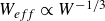 $W_{eff} \propto W^{-1/3}$
) for the FENE-P model, for any non-zero
 $\beta$
and
 $W \gt L$
. Thus, owing to shear thinning, even if the bare Weissenberg number is increased, the effective Weissenberg number attains a maximum of
 $O(L)$
and either plateaus (for FENE-CR) or decreases (for FENE-P) thereafter. That is, the largest value achieved by
 $W_{eff}$
is
 $O(L)$
in both FENE models. Oldroyd-B-based predictions are therefore expected to be valid only for
 $W \ll L$
, and are likely to become progressively less accurate as
 $W$
exceeds
 $L$
. Now, for the specific case of the elastic centre-mode instability, the Oldroyd-B model yields a threshold
 $W \sim 10^3$
(Khalid et al. Reference Khalid, Shankar and Subramanian2021b
). Clearly,
 $W_{eff} \ll W$
if
 $L \lt 10^3$
, implying that
 $L$
must be comparable to or greater than
 $O(10^3)$
for the centre-mode instability to persist in a largely unchanged form, within the FENE-P or FENE-CR framework.
It is useful therefore to estimate the molecular weight of polymers for which
 $L \gt 10^3$
. If the polymer molecule is modelled as an effectively freely jointed chain with
 $N_K$
segments of Kuhn length
 $l_K$
, then
 $L = ( l_K N_K)/(l_K \sqrt {N_K})$
, or
 $ L = \sqrt {N_K}$
. Each Kuhn segment typically consists of
 $N_m =5{-}10$
monomer repeat units (referred to as the ‘characteristic ratio’ in polymer physics; Larson Reference Larson1988; Rubinstein & Colby Reference Rubinstein and Colby2003), implying
 $N_K = N_p/N_m$
, where
 $N_p$
is the actual number of monomer units (the ‘degree of polymerisation’). The polymer molecular weight is
 $M_w = M_m N_p$
, where
 $M_m$
is the monomer molecular weight, so
 $N_K = M_w/(M_m N_m)$
. This yields
 $L = \sqrt {M_w/(M_m N_m)}$
, implying that in order for
 $L$
to be greater than
 $10^3$
, we must have
 $M_w /(M_m N_m) \gt 10^6$
. On using
 $N_m \sim 5$
,
 $M_m \sim 70$
g mol
 $^{-1}$
(corresponding to the polyacrylamide used in experiments of Choueiri et al. Reference Choueiri, Lopez, Varshney, Sankar and Hof2021), one obtains
 $M_w \gt 3.5 \times 10^8$
g mol
 $^{-1}$
for the original elastic centre-mode instability (Khalid et al. Reference Khalid, Shankar and Subramanian2021b
) to be observed; this is likely higher than the highest molecular weight polyacrylamide used in experiments (
 $M_w = 1.8 \times 10^7$
g mol
 $^{-1}$
; Neelamegam, Shankar & Das Reference Neelamegam, Shankar and Das2013). Thus one expects the original centre-mode instability to be suppressed (stabilised) for polymers with
 $M_w \lt 3.5 \times 10^8$
g mol
 $^{-1}$
; an analysis of what happens for lower
 $M_w$
values will need to account for finite extensibility effects.
The stabilising role of finite extensibility has previously been demonstrated for the hoop-stress-driven instability in the cone-and-plate geometry, using the FENE-CR model, by Öztekin et al. (Reference Öztekin, Brown and McKinley1994), and for wall-mode instabilities in pressure-driven channel flow by Sureshkumar & Beris (Reference Sureshkumar and Beris1995); wall modes in the latter instance are a class of eigenmodes with phase speeds
 $c_r \rightarrow 0$
at high
 $Re$
(see Chaudhary et al. (Reference Chaudhary, Garg, Shankar and Subramanian2019) for a detailed discussion of the elastoinertial eigenspectrum). Rather intriguingly, and in direct contrast to the expected stabilising role of finite extensibility, the recent effort by Buza et al. (Reference Buza, Page and Kerswell2022) has shown, using the FENE-P model, that viscoelastic channel flow is linearly unstable to a centre mode at
 $Re = 0$
, for
 $W \sim O(100)$
,
 $L \sim O(10^2)$
and
 $\beta = 0.98$
; the Oldroyd-B model predicts the centre mode to be stable for this
 $\beta$
regardless of
 $W$
(Khalid et al. Reference Khalid, Shankar and Subramanian2021b
).
Motivated by the above considerations, in the present study, we provide a comprehensive account of the effect of finite extensibility, both on the elastoinertial (Khalid et al. Reference Khalid, Chaudhary, Garg, Shankar and Subramanian2021a
) and elastic (Khalid et al. Reference Khalid, Shankar and Subramanian2021b
) centre-mode instabilities for viscoelastic channel flow, using the FENE-CR and FENE-P models. We compare and contrast the results obtained using these two models, while also augmenting the FENE-P results of Buza et al. (Reference Buza, Page and Kerswell2022) by probing a more extensive region in the relevant parameter space. Based on the steady shear rheology, it might be anticipated that both FENE models yield qualitatively similar stability results, especially in the limit of very dilute solutions (e.g.
 $\beta \gt 0.98$
) – the regime pertaining to the centre-mode instability predicted within the FENE-P framework (Buza et al. Reference Buza, Page and Kerswell2022). This is because even though the FENE-P model exhibits shear thinning of
 $\eta _p$
, while FENE-CR does not, any shear thinning of the polymer viscosity is
 $O(1 - \beta )$
, and becomes irrelevant for
 $\beta \rightarrow 1$
(this irrelevance being accentuated for large
 $W$
by shear thinning). Against this expectation, we show that the two FENE models exhibit strikingly different stability characteristics for the centre-mode instability.
The rest of this paper is organised as follows. Section 2 provides the governing equations and base-state quantities for both FENE-P and FENE-CR models, and a brief outline of the numerical procedure used to solve the linearised governing equations. The details of the linearised equations for small-amplitude perturbations are provided in Appendices A and B. In § 3, we discuss the effect of finite extensibility, within the FENE-P framework, on the elastoinertial instability (Khalid et al. Reference Khalid, Chaudhary, Garg, Shankar and Subramanian2021a
) at finite
 $Re$
(§§ 3.1 and 3.2), which is followed by a discussion of its effect on the purely elastic instability (Khalid et al. Reference Khalid, Shankar and Subramanian2021b
) at
 $Re = 0$
(§ 3.3). Analogous results obtained using the FENE-CR model are discussed in § 4. Finally, the salient conclusions and open questions are provided in the concluding § 5.
2. Problem formulation
The flow configuration considered here, as in our earlier efforts (Khalid et al. Reference Khalid, Chaudhary, Garg, Shankar and Subramanian2021a
,Reference Khalid, Shankar and Subramanian
b
), is pressure-driven channel flow between two rigid plates separated by
 $ 2H$
, with the fluid rheology being governed by the FENE-P or FENE-CR models. In the following discussion, velocities are non-dimensionalised using
 $U_{max}$
, the centreline maximum speed corresponding to the Oldroyd-B fluid driven by the same pressure gradient, lengths using the channel half-width
 $H$
, time using
 $H/U_{max}$
, and components of the stress tensor and pressure using
 $ \eta _{t0} U_{max}/H$
; here,
 $ \eta _{t0} = \eta _{p0} + \eta _s$
is the zero-shear (total) solution viscosity,
 $ \eta _{p0}$
is the zero-shear polymer viscosity, and
 $ \eta _s$
is the (Newtonian) solvent viscosity.
The dimensionless continuity and momentum equations are given by
 \begin{equation} \nabla \cdot \mathbf {u}=0, \quad Re \left (\frac {\partial \mathbf {u}}{\partial t}+ \mathbf {u}\cdot \nabla \, \mathbf {u} \right )=-\nabla {p}+ \nabla \cdot \boldsymbol {\tau } + {\beta } \,\nabla ^2 \, \mathbf {u} \, , \end{equation}
where
 $\mathbf {u}$
,
 $p$
and
 $\boldsymbol {\tau }$
are, respectively, the (non-dimensional) velocity, pressure and polymer stress fields,
 $\beta = \eta _s/\eta _{t0}$
, and
 $ Re$
is the Reynolds number based on
 $ U_{max}$
,
 $ H$
and
 $\eta _{t0}$
.
2.1. The FENE-P and FENE-CR models
In these models, the dilute polymer solution is again considered to be a suspension of non-interacting elastic dumbbells in a Newtonian solvent, as for the Oldroyd-B case, but with each dumbbell consisting of two beads connected by a nonlinear entropic spring. The polymer conformation is defined by the bead connector vector
 $\boldsymbol {Q}$
. In the FENE dumbbell, the (dimensional) force-extension relation characterising the entropic elasticity of the spring is given by
 $\boldsymbol {F}_c = ({H_{sp} \boldsymbol {Q}})/{1 -(|\boldsymbol {Q}|/Q_{max})^2}$
, where
 $H_{sp}$
is the (equilibrium) spring constant, with the force diverging in the limit
 $|\boldsymbol {Q}| \to Q_{max}$
. Here,
 $Q_{max}$
is the fully-stretched contour length of the polymer molecule. (Henceforth, the connector vector is rendered dimensionless using
 $\sqrt {(k_B T/H_{sp})}$
, and we continue to represent its non-dimensional analogue using
 $ \boldsymbol {Q}$
.) As mentioned in the Introduction, the nonlinear functional dependence on
 $\boldsymbol {Q}$
precludes the derivation of a closed-form constitutive relation for the stress. The configurational average involved in the stress (defined below), when applied to the underlying kinetic (Smoluchowski) equation, leads to a coupling to higher-order moments, and thence to an infinite moment hierarchy.
In order to obtain a closed-form constitutive equation, Peterlin (Bird et al. Reference Bird, Dotson and Johnson1980; Herrchen & Ottinger Reference Herrchen and Ottinger1997) replaced the
 $\boldsymbol {Q}$
-dependent nonlinear factor in the FENE spring force by its ‘pre-averaged’ equivalent, leading to the FENE-P model. This results in the following (dimensionless) relation between the polymeric stress
 $\boldsymbol {\tau } = \langle \boldsymbol {F}_c \boldsymbol {Q} \rangle$
and the conformation tensor
 $ \boldsymbol {C} = \langle \boldsymbol {Q} \boldsymbol {Q} \rangle$
:
 \begin{equation} \boldsymbol {\tau }=\frac {1-\beta }{W} (f(C_{kk}) \, \boldsymbol {C}-\boldsymbol {I}), \end{equation}
where
 $\langle \cdot \rangle$
represents the aforementioned configurational average. In (2.2),
 $ W = \lambda U_{max}/H$
is the Weissenberg number,
 $ C_{kk} = \text{tr}(\boldsymbol {C})$
, and
 $\boldsymbol {I}$
is the identity tensor representing the isotropic distribution of dumbbell conformations at equilibrium. The Peterlin closure function
 $ f(C_{kk})$
is defined as
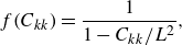 \begin{equation} f(C_{kk}) = \frac {1}{1-{C_{kk}}/{L^2}} , \end{equation}
where
 $ L^2 = Q_{max}^2/(k_B T/H_{sp})$
is the dimensionless parameter mentioned in the Introduction that characterises the maximum extensibility of polymer chains;
 $C_{kk} = Q_{eq}^2$
for
 $W = 0$
, with
 $Q_{eq}^2 = (3k_B T /H) L^2/(L^2 + 5)$
being the mean square extension at equilibrium. The Oldroyd-B model is obtained in the limit
 $L \to \infty$
(
 $f \to 1$
), when
 $\boldsymbol {F}_c$
becomes proportional to
 $\boldsymbol {Q}$
, implying a Hookean spring. It is worth noting (Alves, Oliveira & Pinho Reference Alves, Oliveira and Pinho2021; Davoodi et al. Reference Davoodi, Zografos, Oliveira and Poole2022) that there are (slightly) different variants of the FENE-P model prevalent in the literature, and the present work employs the version used by Zhang et al. (Reference Zhang, Lashgari, Zaki and Brandt2013) (see also Housiadas & Beris Reference Housiadas and Beris2003) in order to facilitate benchmarking of our numerical procedure. Importantly, the variants differ only by terms of
 $O(1/L^2)$
, and must therefore yield virtually identical results for
 $L \gtrsim O(10)$
. Herein, our focus is on the latter regime, implying that arguments with regard to shear thinning, in the Introduction, apply regardless of the particular variant used. The stability results detailed below should likewise be valid for the other FENE-P variants.
To describe the nonlinear rheology of Boger fluids (James Reference James2009), which exhibit negligible shear thinning of viscosity (owing to the presence of a highly viscous solvent), Chilcott & Rallison (Reference Chilcott and Rallison1988a
) proposed a model that leads to a shear-rate-independent viscosity, but retains the shear-rate dependence of the first normal stress coefficient. This is achieved by an (ad hoc) insertion of another factor
 $f$
multiplying the identity tensor in (2.2), leading to the FENE-CR model, with the stress given by
 \begin{equation} \boldsymbol {\tau } = (1-\beta ) \frac {f(C_{kk}) \, (\boldsymbol {C} - \boldsymbol {I})}{W}\, . \end{equation}
The evolution of the conformation tensor for both the aforementioned models can be expressed as
 \begin{eqnarray} (1-\beta ) \left (\frac {\partial \boldsymbol {C}}{\partial t}+(\mathbf {u}\cdot \nabla )\boldsymbol {C}-(\nabla \mathbf {u})^{\rm T} \cdot \boldsymbol {C}- \,\boldsymbol {C} \cdot (\nabla \mathbf {u})\right )= - \boldsymbol {\tau } , \end{eqnarray}
where
 $\boldsymbol {\tau }$
on the right-hand side takes the forms given in (2.2) and (2.4) for the FENE-P and FENE-CR models, respectively. As in the Oldroyd-B model, the terms within the parentheses on the left-hand side of (2.5) represent the upper-convected derivative operating on the conformation tensor
 $ \boldsymbol {C}$
, corresponding to an affine deformation of the underlying dumbbells in the limit
 $W \rightarrow \infty$
(i.e. in the absence of the restoring spring force).
2.2. Base-state velocity and stress distributions
In what follows, we use uppercase Roman alphabets to denote base-state quantities corresponding to the velocity field, stress field and components of the conformation tensor. For the Oldroyd-B fluid, on account of the shear-rate-independent viscosity, the steady unidirectional velocity profile for pressure-driven channel flow is the same as its Newtonian counterpart, the plane Poiseuille profile, with
 $U(z) = (1-z^2)$
. However, unlike the Newtonian case, the Oldroyd-B fluid exhibits a first normal stress difference
 $(T_{xx} - T_{zz}) = 8W^2z^2$
, and second normal stress difference
 $(T_{zz} - T_{yy}) = 0$
. In the coordinate-specific expressions above, and those that appear below,
 $x$
,
 $y$
and
 $z$
are, respectively, the flow (streamwise), vorticity (spanwise) and wall-normal directions, with perturbation velocity components denoted by
 $u$
,
 $w$
and
 $v$
.
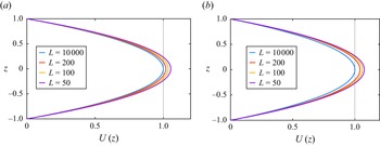
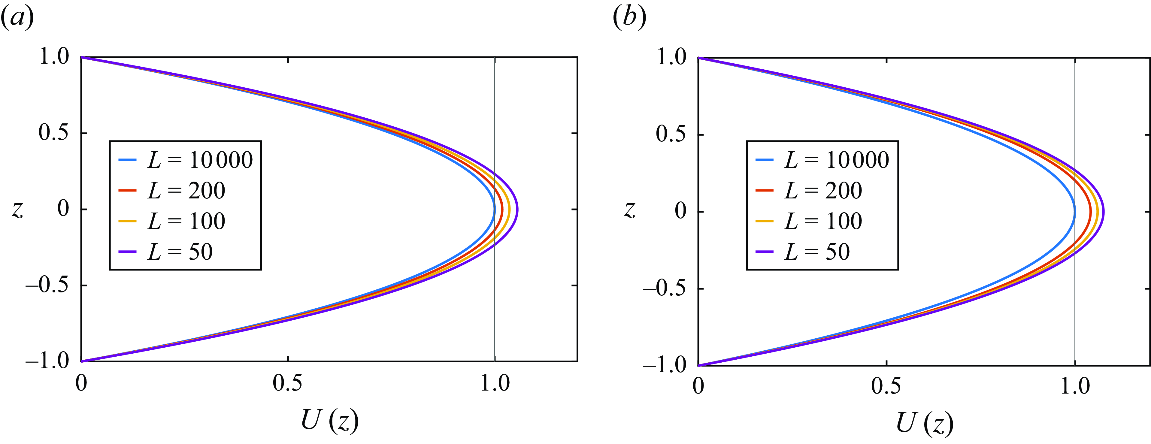
Base-flow velocity profiles for the FENE-P fluid for
 $\beta = 0.9$
at different
 $L$
values, for
 $W = 60$
and
 $150$
.
2.2.1. The FENE-P model
Unlike the Oldroyd-B model, shear thinning leads to the FENE-P model yielding a non-parabolic velocity profile (Cruz, Pinho & Oliveira Reference Cruz, Pinho and Oliveira2005; Zhang et al. Reference Zhang, Lashgari, Zaki and Brandt2013) given by
 \begin{eqnarray} U(z)=-\frac {1}{2\beta }\frac {{\rm d}p}{{\rm d}x}(1-z^2)-\frac {1-\beta }{\beta }\frac {3}{8B}( (F_+G_-)|_{-1}^{z} + (F_-G_+)|_{-1}^{z})\, , \end{eqnarray}
where
 \begin{eqnarray} F_+=(Bz + \sqrt {B^2z^2+A^3})^{1/3},\quad F_-=(Bz - \sqrt {B^2z^2+A^3})^{1/3}, \end{eqnarray}
 \begin{eqnarray} G_+=3Bz + \sqrt {B^2z^2+A^3},\quad G_-=3Bz - \sqrt {B^2z^2+A^3}\, , \end{eqnarray}
and
 \begin{equation} A=\dfrac {L^2}{6W^2}\left (1 + \dfrac {3}{L^2}+\dfrac {1-\beta }{\beta }\right ), \quad B=\dfrac {L^2}{4 W^2}\,\dfrac {{\rm d}p}{{\rm d}x}\,\dfrac {1}{\beta } . \end{equation}
Since the velocity scale (
 $U_{max}$
) used is the maximum speed for plane Poiseuille flow of an Oldroyd-B fluid,
 ${\rm d}p/{\rm d}x = -2$
in (2.6). Figure 1 shows the velocity profiles at different
 $L$
values for two different
 $W$
values. As
 $L$
is decreased, the maximum speed increases above unity owing to shear thinning.
In general,
 $U(z)$
in (2.6) is a function of
 $W$
,
 $L$
and
 $\beta$
. However, a notable feature in the above expressions is that, except for the
 $3/L^2$
term in the expression for
 $A$
in (2.9),
 $U(z)$
depends on
 $W$
and
 $L$
only through the combination
 $W/L$
. For
 $L \gt 10$
, the term
 $3/L^2$
is negligible compared to the other two terms in
 $A$
, and velocity profiles for different values of
 $W$
and
 $L$
, such that
 $W/L$
is constant, must therefore be virtually identical. Indeed, instead of using (2.3), if we use the FENE-P variant where
 $f = (L^2 - 3)/(L^2 - C_{kk})$
(see Alves et al. (Reference Alves, Oliveira and Pinho2021) for the prevalent FENE-P variants), then the
 $3/L^2$
term is absent, and the aforementioned collapse is exact for any
 $L$
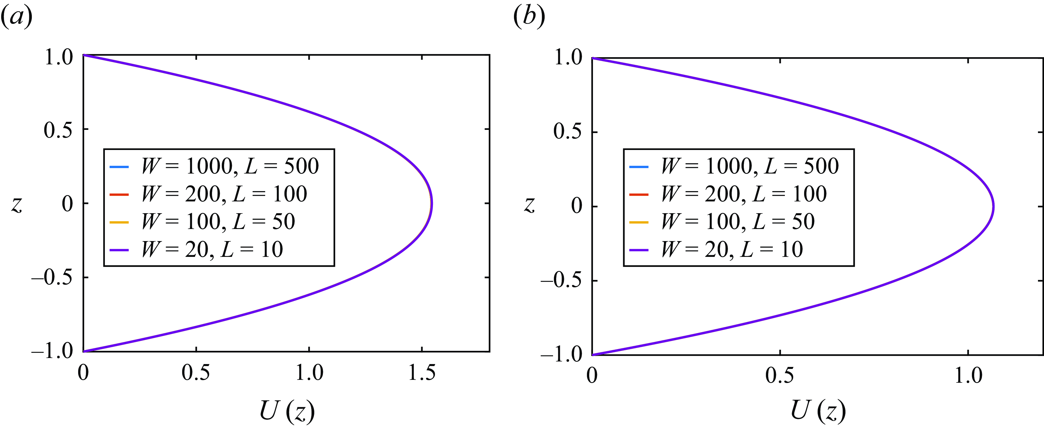
(Tej, Mohanty & Shankar Reference Tej, Mohanty and Shankar2024). This collapse is analogous to that of the polymer contribution to viscosity
 $\eta _p$
and the first normal stress coefficient
 $\Psi _1$
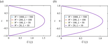
, for plane Couette flow, demonstrated by Yamani & McKinley (Reference Yamani and McKinley2023), and is illustrated in figure 2 for different
 $W$
and
 $L$
. The collapse generally holds for steady unidirectional shear flows, including pipe flow (Tej et al. Reference Tej, Mohanty and Shankar2024). However, as pointed out by Yamani & McKinley (Reference Yamani and McKinley2023), it breaks down for purely extensional flows, due to the two- or three-dimensional nature of the velocity field in such flows.
Master curves for base-flow velocity profiles of a FENE-P fluid at a fixed
 $W/L$
obtained for different pairs
 $(W,L)$
at (a)
 $\beta=0.5$
and (b)
 $\beta=0.9$
.
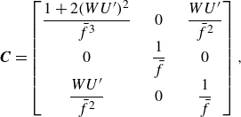
The base-state conformation tensor is given by
 \begin{equation} {\boldsymbol {C}} = \begin{bmatrix} \dfrac {1 + 2 (W U^{\prime})^2}{\bar {f}^3} &\quad 0 &\quad \dfrac {W U^{\prime}}{\bar {f}^2} \\ 0 &\quad \dfrac {1}{\bar {f}} &\quad 0 \\ \dfrac {W U^{\prime}}{\bar {f}^2} &\quad 0 &\quad \dfrac {1}{\bar {f}} \end{bmatrix} , \end{equation}
where
 $U^{\prime} = {\rm d}U/{\rm d}z$
, and
 $\bar {f}$
(with overbar denoting the base-state) satisfies the cubic relation
 $\bar {f}^3 -\bar {f}^2 -({2 W^2 (U^{\prime})^2})/{L^2} = 0$
. Of the three roots of this cubic, only one is physically admissible (i.e. real-valued). The base-state polymeric stress tensor, obtained from (2.2), is
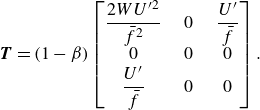 \begin{equation} {\boldsymbol {T}} = (1-\beta ) \begin{bmatrix} \dfrac {2 W U^{\prime2}}{\bar {f}^2} &\quad 0 &\quad \dfrac {U^{\prime}}{\bar {f}} \\ 0 &\quad 0 &\quad 0 \\ \dfrac {U^{\prime}}{\bar {f}} &\quad 0 &\quad 0 \end{bmatrix}. \end{equation}
Since the expression for
 $\bar {f}$
contains
 $U^{\prime}$
, its presence in
 $T_{xz}$
and
 $T_{xx}$
is the reason for the shear-rate dependence of both viscosity and the first normal stress coefficient.
2.2.2. FENE-CR model
The base-state velocity profile in the FENE-CR model is identical to the plane Poiseuille flow profile due to the shear-rate independent viscosity. The conformation and polymeric stress tensors in the base state are given by
 \begin{equation} \boldsymbol {C} = \begin{bmatrix} 1+2\left (\dfrac {WU^{\prime}}{\overline {f}} \right )^2 &\quad 0 &\quad \dfrac {WU^{\prime}}{\overline {f}} \\ 0 &\quad 1 &\quad 0 \\ \dfrac {WU^{\prime}}{\overline {f}} &\quad 0 &\quad 1 \end{bmatrix} ,\quad {\boldsymbol {T}}= (1-\beta ) \begin{bmatrix} 2\left (\dfrac {W}{\overline {f}} \right )U^{\prime} &\quad 0 &\quad U^{\prime} \\ 0 &\quad 0 &\quad 0 \\ U^{\prime} &\quad 0 &\quad 0 \end{bmatrix}\, . \end{equation}
Here,
 $\bar {f}$
satisfies a quadratic equation whose physically valid solution is
 \begin{equation} \overline {f} = \dfrac {L^2 + \sqrt {L^4 + 8(WU^{\prime})^2(L^2 - 3)}}{2(L^2 - 3)}\,. \end{equation}
While
 $\bar {f}$
above involves
 $U^{\prime}$
similar to the FENE-P model, the absence of the
 $1/\bar {f}$
factor in
 $T_{xz}$
in (2.12), leads to the viscosity being independent of the shear rate. Its presence in
 $T_{xx}$
, however, results in a shear-rate-dependent first normal stress coefficient.
2.3. Linearised equations for small perturbations
A temporal linear stability analysis is carried out using the two models above, by writing the different field variables as the sum of their base-state values (denoted by uppercase alphabets) and superposed infinitesimal perturbations (lowercase alphabets with primes):
 $\mathbf {u}=\mathbf {U}+\mathbf {u}^{\prime}$
,
 $p=P+p^{\prime}$
,
 $\boldsymbol {\tau }=\mathbf {T}+\boldsymbol {\tau }^{\prime}$
 $\mathbf {c}=\mathbf {C} + \boldsymbol {c}^{\prime}$
. After substitution of these forms, the governing equations are linearised about the base state; similar to our earlier effort (Khalid et al. Reference Khalid, Chaudhary, Garg, Shankar and Subramanian2021a
,Reference Khalid, Shankar and Subramanian
b
), we consider only two-dimensional perturbations, varying only in the streamwise and wall-normal directions. The use of two-dimensional perturbations is justified for Oldroyd-B fluids (within a modal stability analysis), owing to the existence of a Squire’s theorem, which states that corresponding to each unstable three-dimensional disturbance at given
 $Re$
,
 $W$
, there is a two-dimensional unstable mode at a lower
 $Re$
,
 $W$
, with a larger growth rate (Bistagnino et al. Reference Bistagnino, Boffetta, Celani, Mazzino, Puliafito and Vergassola2007). We are not aware of an extension of the Squire’s theorem for the FENE-P and FENE-CR models, but nevertheless assume two-dimensional disturbances in these cases. The two-dimensional perturbations are taken to be individual Fourier modes of the form
 $ f^{\prime}(x,z,t)=\tilde {f}(z)\exp[{\rm i}k(x-ct)]$
, where
 $f^{\prime}$
is any of the perturbation fields,
 $ \tilde {f}(z)$
is the eigenfunction,
 $ k$
is the real streamwise wavenumber, and
 $ c= c_r + {\rm i}c_i$
is the complex eigenvalue, with
 $c_r$
the wave speed, and
 $c_i$
the growth rate, and the flow being temporally unstable when
 $ c_i \gt 0$
. The linearised governing equations for both models are provided in Appendices A and B.
The linearised system is solved using a spectral collocation method, as explained in our earlier effort (Khalid et al. Reference Khalid, Chaudhary, Garg, Shankar and Subramanian2021a
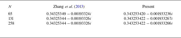
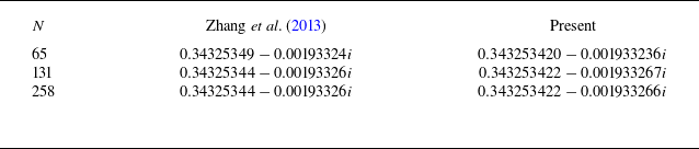
). To benchmark our numerical implementation for the FENE-P model, we have compared results from our procedure with those of Zhang et al. (Reference Zhang, Lashgari, Zaki and Brandt2013); the eigenvalues are in good agreement (table 1). In addition, we have benchmarked the recent results of Buza et al. (Reference Buza, Page and Kerswell2022) (personal communication) both at finite
 $ Re$
and in the creeping-flow (
 $ Re =0$
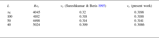
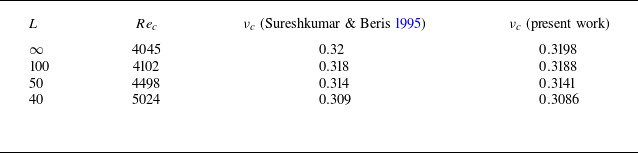
) limit. Our FENE-CR results were benchmarked with those given in table 6 of Sureshkumar & Beris (Reference Sureshkumar and Beris1995); see table 2.
Validation of our FENE-P results with those of Zhang et al. (Reference Zhang, Lashgari, Zaki and Brandt2013) for viscoelastic channel flow at
 $ Re =3960,\ \beta =0.5,\ W=3.96,\ k=1.15,\ L = 60$
.
Validation of our FENE-CR results with those of Sureshkumar & Beris (Reference Sureshkumar and Beris1995): critical Reynolds number
 $Re_c$
and critical frequency
 $\nu _c$
at different
 $L$
.
3. Role of finite extensibility using the FENE-P model
Before proceeding to discuss the effect of finite extensibility on the centre-mode instability, it is useful to recapitulate the salient features of this instability, obtained within the Oldroyd-B framework, for viscoelastic channel flow (Khalid et al. Reference Khalid, Chaudhary, Garg, Shankar and Subramanian2021a
). The instability is characterised by modes with phase speeds very close to the base-state maximum and is governed by the dimensionless parameters
 $Re$
,
 $E$
(or
 $W$
) and
 $\beta$
for an Oldroyd-B fluid. For
 $0.5 \lt \beta \lt 0.990552$
, the critical Reynolds number is
 $Re_c \propto E^{-3/2}$
for
 $E \ll 1$
; the instability is absent beyond a threshold
 $E$
of order unity (which is a function of
 $\beta$
) owing to
 $Re_c$
diverging rapidly near this threshold. However, for
 $\beta \gt 0.990552$
, the instability continues to
 $E \rightarrow \infty$
, with
 $Re_c \propto E^{-1}$
in this limit. This latter scaling implies that a threshold
 $W$
governs the instability in the limit
 $Re \rightarrow 0$
, thereby indicating that for
 $\beta \gt 0.990552$
, the original elastoinertial centre-mode instability smoothly morphs into a purely elastic one, with the latter persisting even in the absence of fluid inertia. We note in passing that there are interesting differences between the channel and pipe-flow centre-mode instabilities: the instability is absent for
 $\beta \lt 0.5$
for channel flow as indicated above, while continuing to exist down to very low
 $\beta$
values for pipe flow (Chaudhary et al. Reference Chaudhary, Garg, Subramanian and Shankar2021). Despite this wider range of unstable
 $\beta$
, the instability is present only for
 $Re \gtrsim 63$
, precluding the possibility of an elastic instability in the pipe flow geometry.
Below, we first examine the effect of finite extensibility on the elastoinertial instability using the FENE-P model, and then proceed to discuss its effect on the purely elastic instability. In the next section, we discuss the role of finite extensibility within the framework of the FENE-CR model.
3.1. Eigenspectra for the elastoinertial centre mode
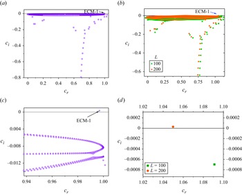
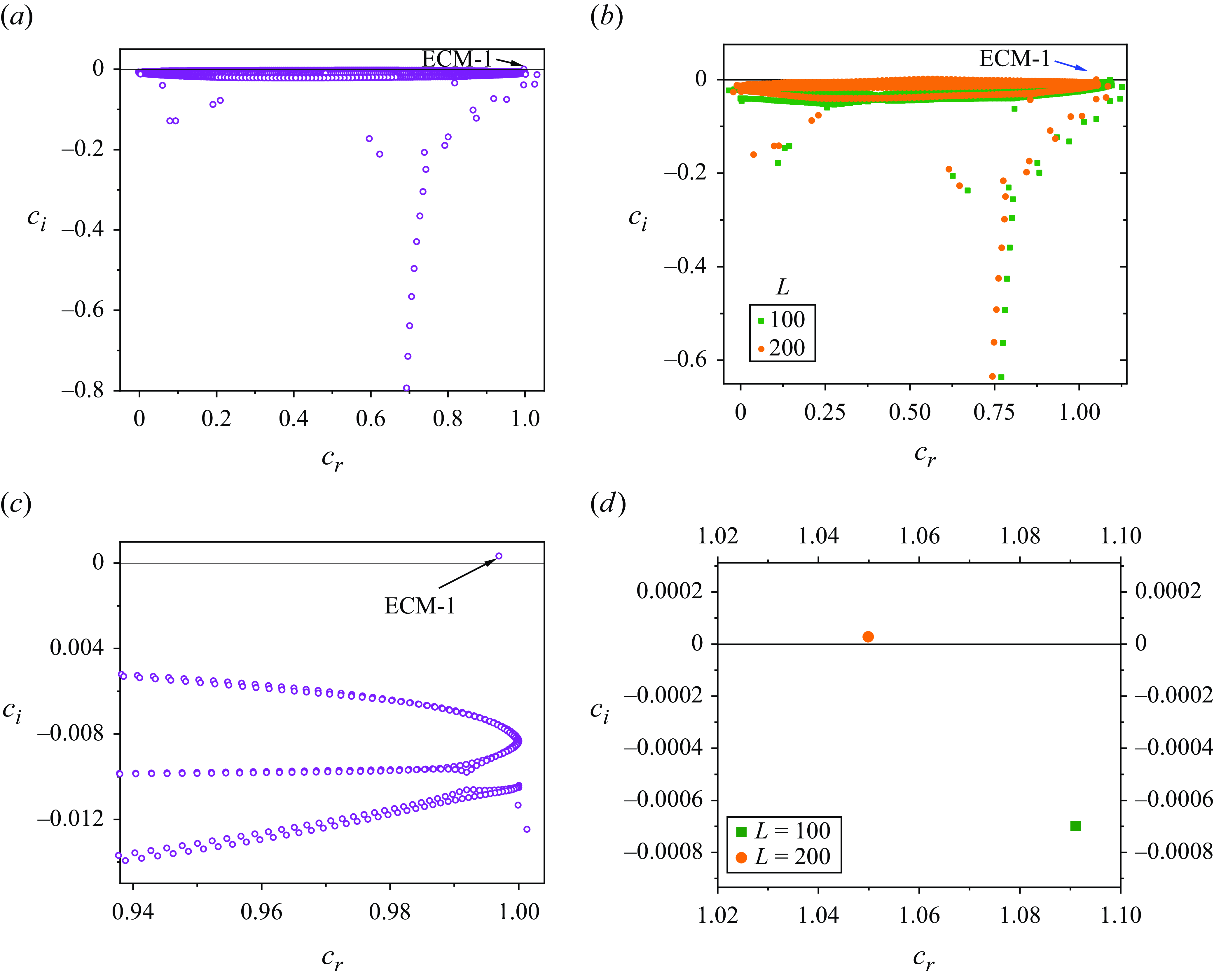
Figure 3 shows the spectra obtained for both Oldroyd-B (figures 3
a,c) and FENE-P fluids (figures 3
b,d), the latter for
 $L = 200$
and
 $100$
, for
 $E = 0.1$
. In figures 3(a) and 3(c), the Oldroyd-B limit is obtained from the FENE-P fluid by taking
 $L = 10^4$
; we show subsequently (in figure 4) that this value of
 $L$
is sufficient to capture the Oldroyd-B spectrum accurately, the spectrum being virtually invariant to a further increase in
 $L$
. As is well known, viscoelastic shearing flows, including the channel flow configuration examined here, are characterised by the presence of singular continuous spectra, whose (stable) eigenvalues lie on a line segment in the
 $c_r$
–
 $c_i$
plane. However, owing to the singular nature of the associated eigenfunctions, the eigenvalues belonging to the continuous spectra are not fully converged for any finite
 $N$
, with the theoretical line segment only being resolved as a balloon in the spectral method, the balloon extending to
 $c_i \gt 0$
if
 $N$
is not large enough. These eigenvalues, which are easily filtered out based on a convergence criterion, are therefore not considered in the ensuing discussion.
Elastoinertial spectra for viscoelastic channel flow (a) in the Oldroyd-B limit (
 $L = 10^4$
), and (b) for finite extensibilities using the FENE-P model (
 $L = 100,\ U_{max,F} = 1.09451$
and
 $L = 200,\ U_{max,F} = 1.05297$
). Data for
 $Re = 800$
,
 $E = 0.1$
,
 $\beta = 0.8$
,
 $k = 1.5$
. (c,d) Zoomed-in regions of (a,b), respectively, near the elastoinertial centre mode (ECM-1).
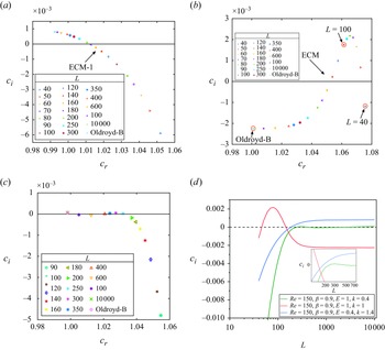
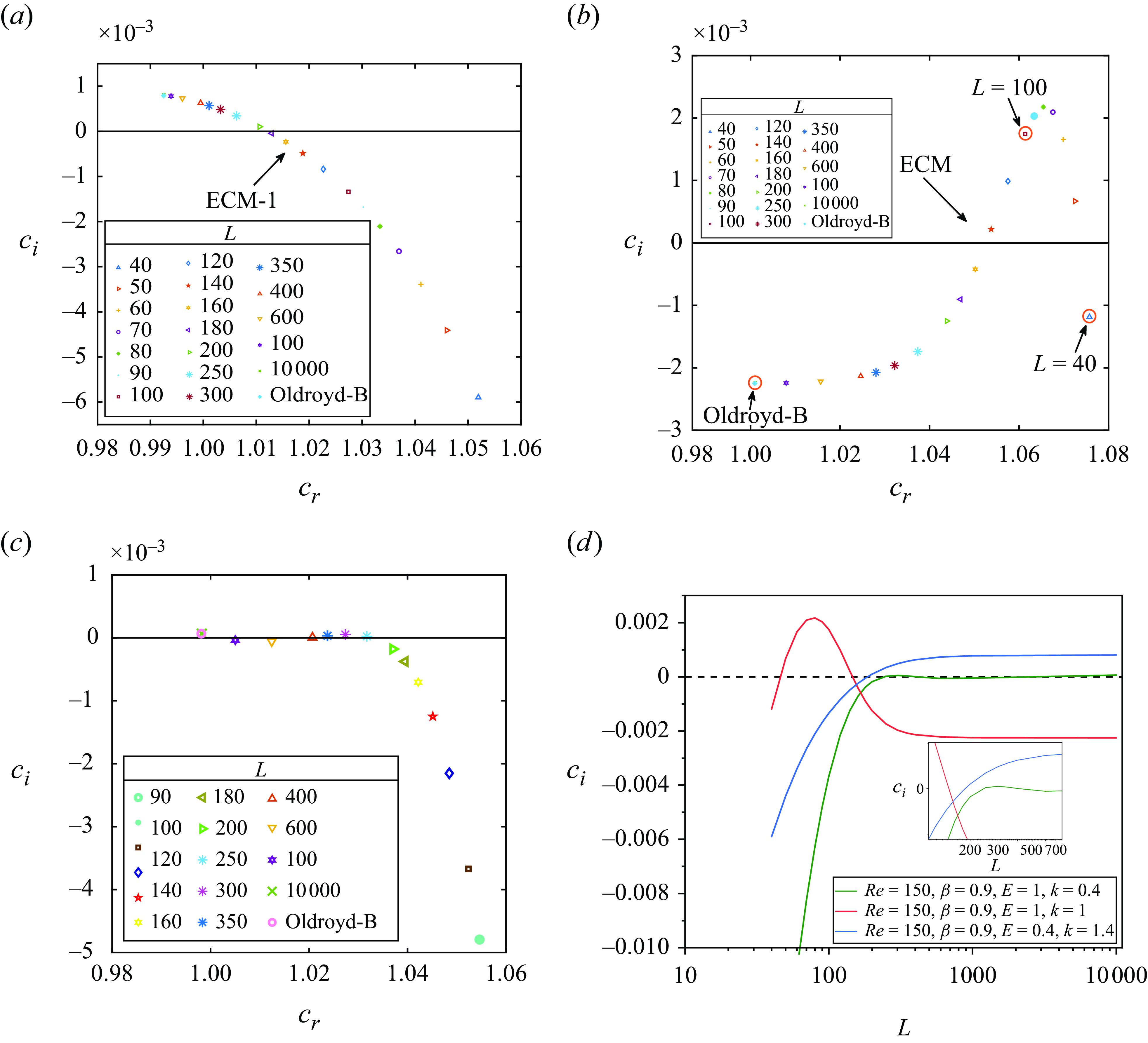
Dual role of finite extensibility on the centre mode illustrated using an enlarged view of the elastoinertial spectra, near the ECM obtained using the FENE-P model. (a)
 $Re = 150$
,
 $E = 0.4$
,
 $\beta = 0.9$
,
 $k = 1.4$
. The ECM is unstable in the Oldroyd-B limit and is monotonically stabilised by a decrease in
 $L$
. (b)
 $Re = 150$
,
 $E = 1$
,
 $\beta = 0.9$
,
 $k = 1$
. The ECM is stable in the Oldroyd-B limit, and is destabilised by an initial decrease in
 $L$
before being stabilised again for sufficiently small
 $L$
. The encircled eigenvalues are the ones for which eigenfunctions are shown in figure 5. (c)
 $Re = 150$
,
 $E = 1$
,
 $\beta = 0.9$
,
 $k = 0.4$
. The ECM is unstable in the Oldroyd-B limit. A decrease in
 $L$
leads to an initial stabilisation, a subsequent destabilisation, and an eventual stabilisation. (d)
 $c_i$
vs.
 $L$
for the adjacent panels. Summary of the results by showing the variation of
 $c_i$
with
 $L$
in (a,b,c).
Figures 3(a) and 3(c), respectively, show the overall spectra for the Oldroyd-B and FENE-P fluids, while figures 3(b) and 3(d) show the enlarged region near the unstable centre mode. Figure 3(c) shows an unstable centre mode with phase speed close to, but a little less than unity, for the Oldroyd-B fluid, the latter value being the base-state maximum. For the FENE-P fluid, figure 3(d) shows that the centre mode is unstable for
 $L = 200$
, while being stable for
 $L = 100$
. The phase speeds of these modes are slightly higher than unity, owing to the maximum velocity for the Oldroyd-B fluid being used as the velocity scale. In figures 3(b) and 3(d),
 $W = 80$
, with
 $W/L = 0.8$
and
 $0.4$
for
 $L = 100$
and
 $200$
, respectively. For such values of
 $W/L$
, figure 3(c) of Yamani & McKinley (Reference Yamani and McKinley2023) shows that the polymer contribution to the viscosity
 $\eta _p$
starts to decrease from its zero-shear value, and for a fixed pressure gradient, the (dimensionless) base-state maximum (
 $U_{max,F}$
) for the FENE-P fluid therefore increases beyond that for an Oldroyd-B fluid (i.e.
 $U_{max,F} \gt 1$
; see caption to figure 3). Because the phase speed of the centre-mode instability is very close to
 $U_{max,F}$
, we find the
 $c_r$
values to be higher than unity for the FENE-P case. Another noteworthy feature in figures 3(c) and 3(d) is that while the centre mode is unstable in the Oldroyd-B limit, it is only marginally unstable for
 $L = 200$
, and is stable for
 $L = 100$
, suggesting a stabilising effect of finite extensibility at the chosen (small)
 $E$
.
We explore the above trend in detail, via a plot of
 $c_r$
versus
 $c_i$
for different
 $L$
, in figure 4(a). The figure shows, for a small
 $E = 0.4$
(slightly higher than
 $E = 0.1$
in figure 3), that decreasing
 $L$
from the Oldroyd-B limit down to
 $L = 40$
has a monotonically stabilising effect. This stabilisation can be rationalised by noting that for
 $W=60$
considered in figure 4(a),
 $W/L$
increases from
 $0$
(Oldroyd-B limit) to
 $1.5$
(
 $L=40$
). As the onset of shear thinning happens for
 $W/L \sim O(1)$
, one expects the shear thinning of
 $\Psi _1$
, and the concomitant decrease of the effective Weissenberg number
 $W_{eff} = \Psi _1 \dot {\gamma }^2/\tau _{xz}$
, to have a stabilising effect. The centre mode is seen to become stable (corresponding to
 $c_i$
crossing zero) for
 $L \leqslant 180$
, with
 $W/L \geqslant 1/3$
.
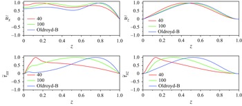
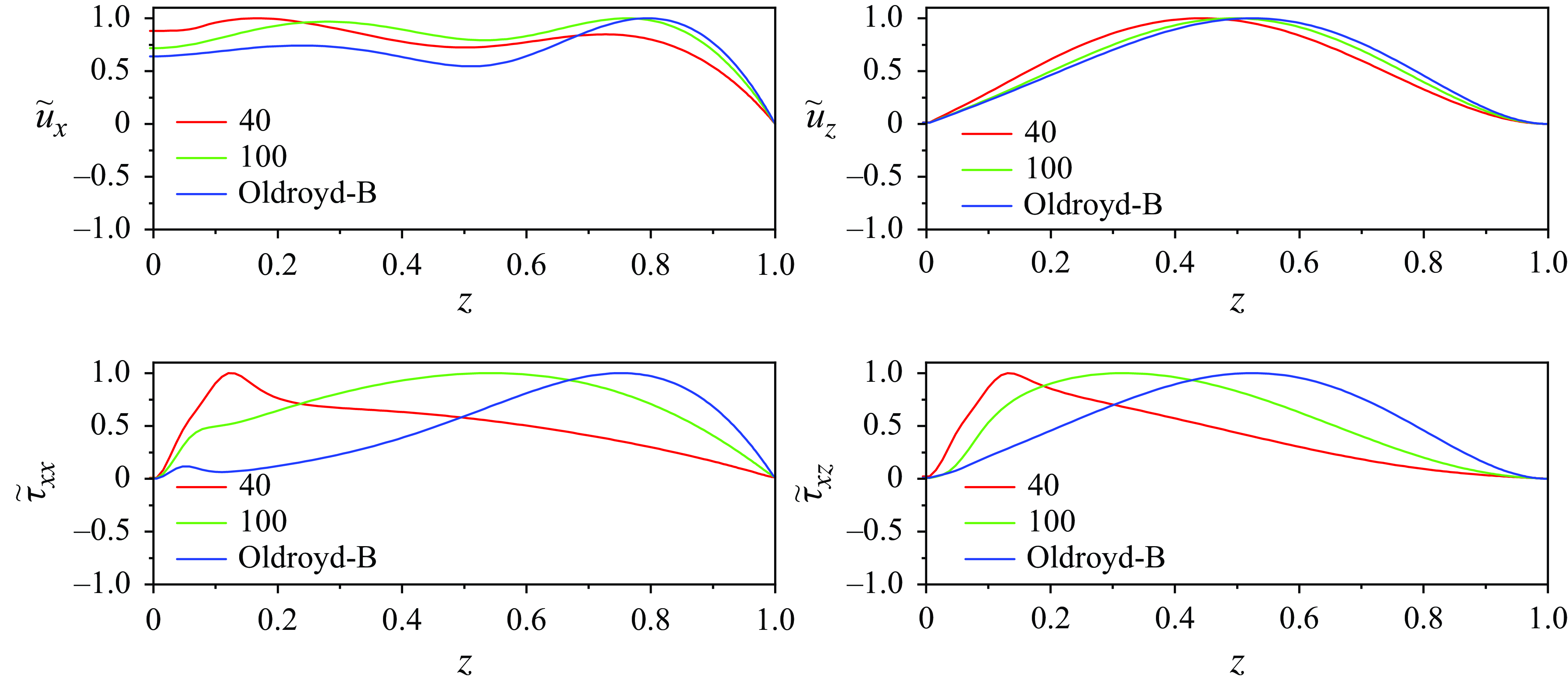
Velocity and stress perturbation eigenfunctions corresponding to the ECM in figure 4, for
 $Re = 150$
,
 $E = 1.0$
,
 $\beta = 0.9$
,
 $k = 1.0$
, for different
 $L$
. All eigenfunctions are shown over the half-channel domain (
 $0 \leqslant z \leqslant 1$
) on account of symmetry. The corresponding eigenvalues are:
 $L = 40$
(
 $U_{max} = 1.08012$
),
 $c = 1.07575 - 0.00118415{\rm i}$
,
 $z_c = 0.066$
;
 $L = 100$
(
 $U_{max} = 1.06042$
),
 $c = 1.06141 + 0.00174635{\rm i}$
,
 $z_c = 0.00315$
; Oldroyd-B (
 $U_{max} = 1$
),
 $c = 1.00097 - 0.00224793{\rm i}$
. Here,
 $z_c$
denotes the critical-layer locations for the stable eigenmodes.
In sharp contrast, figure 4(b) considers a parameter regime where the centre mode is stable in the Oldroyd-B limit; the key difference relative to figure 4(a) is the increased value of
 $E\,(= 1)$
. The centre mode now becomes unstable with decreasing
 $L$
. This counterintuitive destabilising role of finite extensibility is in direct contradiction with the argument of weakened elastic effects due to shear thinning, used above to rationalise the stabilisation at smaller
 $E$
. This prediction is nevertheless consistent with the results of Buza et al. (Reference Buza, Page and Kerswell2022), who also demonstrated the instability of the FENE-P centre mode in parameter regimes where it is stable in the Oldroyd-B limit. The destabilising role of finite extensibility is present over a limited range of
 $L$
values (
 $45 \lt L \lt 150$
), and there is an eventual stabilisation for
 $L \approx 40$
and lower, corresponding to
 $W/L \gt 3.5$
. Thus as
 $L$
is decreased to sufficiently small values (at fixed
 $W$
), the eventual significant increase in
 $W/L$
and the implied approach to the high-shear-rate asymptote renders the argument, based on stabilisation due to finite-extensibility-induced shear thinning, consistent. Crucially, the value of
 $L$
for the polyacrylamide used in the experiments of Choueiri et al. (Reference Choueiri, Lopez, Varshney, Sankar and Hof2021) falls within the above unstable range of
 $L$
values: using
 $M_w = 5 \times 10^6$
g mol
 $^{-1}$
,
 $M_m \approx 70$
g mol
 $^{-1}$
and
 $N_m \sim 5$
in
 $L = \sqrt {M_w/(M_m N_m)}$
yields
 $L \approx 120$
. Thus the predicted destabilisation due to finite extensibility is likely relevant to the observed onset of EIT in the said experiments.
In figure 4(c), corresponding to the same
 $E$
as in figure 4(b) but a smaller
 $k$
, rather remarkably, we see a behaviour with respect to
 $L$
that is doubly non-monotonic. That is, the centre mode is unstable in the Oldroyd-B limit, but stabilises initially with a decrease in
 $L$
. It again becomes unstable for
 $200 \lt L \lt 400$
, before eventually becoming stable for
 $L \lt 200$
. While we do not have a physical argument to explain the rather puzzling destabilising role played by finite extensibility, for the
 $O(1)$
values of
 $W/L$
in figures 4(b) and 4(c), we attempt to isolate the probable reasons by considering the FENE-CR fluid in § 4. Figure 4(d) summarises the contrasting behaviour of
 $c_i$
, as a function of
 $E$
, seen in figures 4(a–c); the inset shows the enlarged region where
 $c_i \gt 0$
(near
 $L \approx 200$
) for
 $k = 0.4$
.
The absolute values of the eigenfunctions for the velocity (
 $\tilde {v}_z$
,
 $\tilde {v}_x$
) and stress (
 $\tilde {\tau }_{xz}$
,
 $\tilde {\tau }_{xx}$
) perturbations, for different
 $L$
values, are shown in figure 5; for reasons related to symmetry (or anti-symmetry) of the field variables, the eigenfunctions are shown only for one-half of the channel. The three values of
 $L$
correspond to the encircled eigenvalues in figure 4(b), and are such that the flow is stable in the Oldroyd-B limit, unstable for
 $L = 100$
, and stable again for
 $L = 40$
. Despite this qualitative difference in the nature of stability, the velocity eigenfunctions are qualitatively similar for both Oldroyd-B and FENE-P models. It is only in the stress eigenfunctions, the
 $\tilde {\tau }_{xx}$
eigenfunction in particular, that one begins to see qualitative differences, with the peak of the FENE-P eigenfunctions being more prominent and localised near the channel centre for the smaller
 $L$
. This localisation points to the development of a critical layer for the stable eigenmodes. Apart from the critical-layer signature, however, there is no clear distinguishing feature between the two FENE-P stress eigenfunctions that might explain the difference in stability.
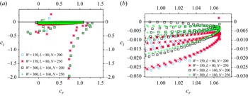
Elastoinertial spectra for
 $(W,L) \equiv (150,80)$
and
 $(300,160)$
such that
 $W/L$
is fixed: data for
 $Re = 150$
,
 $\beta = 0.9$
: (a) overall spectra, (b) zoomed-in spectra. Despite
 $W/L$
being the same, the two spectra are different. For each pair, the spectra are shown for two
 $N$
values in order to ensure convergence of the discrete eigenvalue.
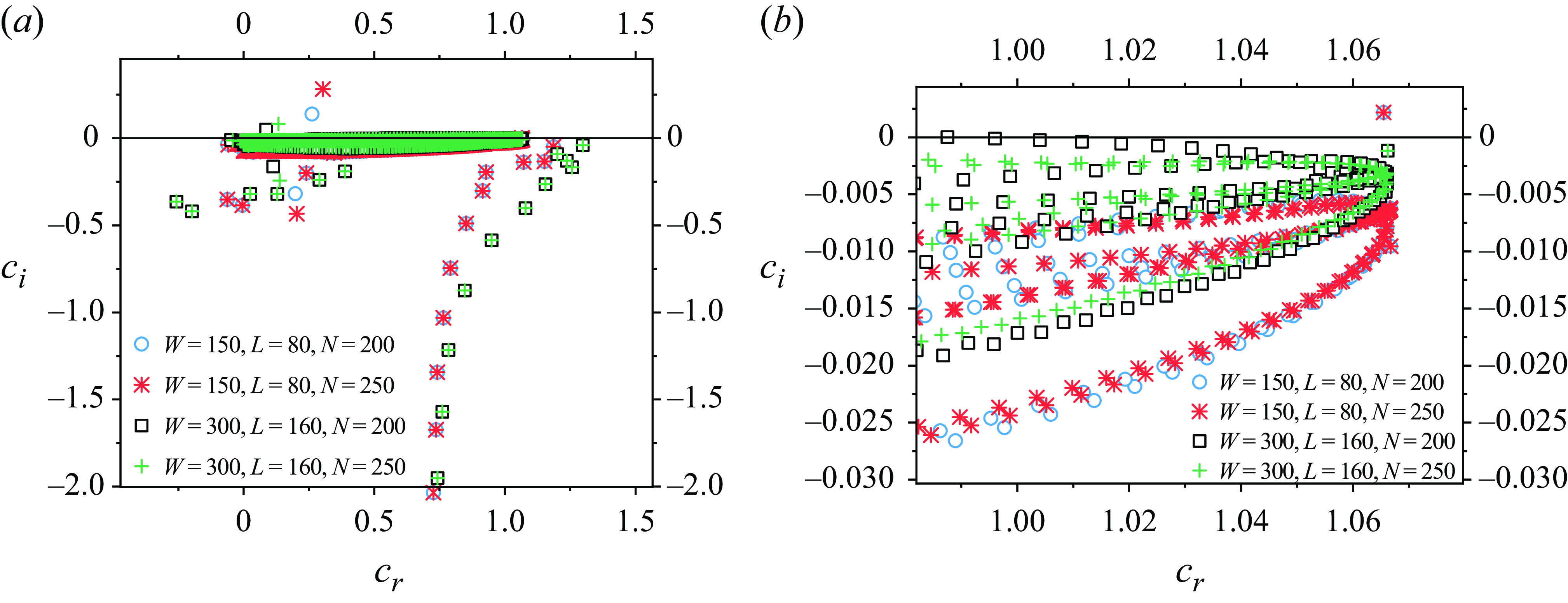
It was argued in § 2.1 that for a fixed
 $\beta$
, the base-state velocity profiles are identical for a given
 $W/L$
. In figure 6, we show the spectra for two
 $(W,L)$
pairs, such that
 $W/L$
is fixed. Despite the base-state profiles being identical for the two cases, their eigenspectra are not, implying that stability is not governed by the combination
 $W/L$
, but by
 $W$
and
 $L$
independently; this is consistent with the form of linearised equations in Appendix A. Indeed, the mode that is unstable for
 $W = 150,\ L = 80$
becomes stable for
 $W = 300,\ L = 160$
. The lack of collapse of spectra with the same
 $W/L$
is because despite the base-state flow being a unidirectional shearing flow, the perturbed flow is not.
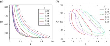
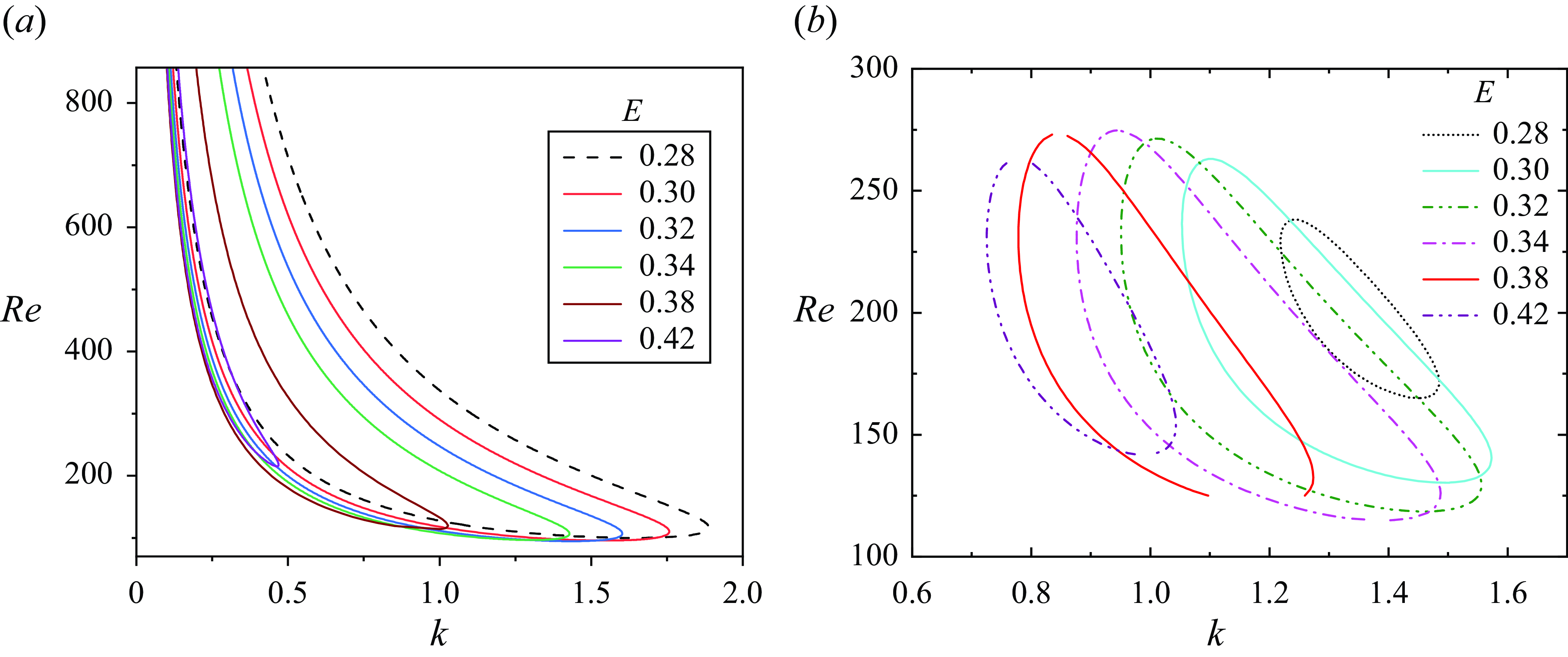
Neutral stability curves in the
 $Re$
–
 $k$
plane for different
 $E$
, for
 $\beta = 0.8$
: (a) Oldroyd-B and (b) FENE-P (
 $L = 70$
). The role of finite extensibility is to suppress the instability at higher
 $Re$
values, leading to a closed unstable region (an ‘island’) in the
 $Re{-}k$
plane. The threshold (minimum)
 $Re$
is largely unaffected by a decrease in
 $L$
for the range of
 $E$
examined.
3.2. Neutral stability curves for the elastoinertial centre mode
The neutral stability curves in the
 $Re$
–
 $k$
plane, for fixed values of
 $E$
and
 $\beta$
, are shown in figure 7 for both Oldroyd-B and FENE-P models. For the Oldroyd-B case, the neutral curves take the form of unstable tongues in the
 $Re$
–
 $k$
plane (Khalid et al. Reference Khalid, Chaudhary, Garg, Shankar and Subramanian2021a
), with the unstable region extending all the way down to
 $k = 0$
, and with the upper and lower branches of each tongue conforming to the scaling
 $Re \propto k^{-1}$
for
 $k\ll 1$
. Within the FENE-P framework, as
 $k$
is decreased, the associated increase in
 $Re$
implies an increase in
 $W$
(since
 $E$
is fixed), thereby making shear thinning important. As already discussed in the previous subsection, the latter leads to a weakening of the elastic forces and an eventual stabilisation. Thus for any finite
 $L$
, one generally expects the unstable neutral tongues, present in the Oldroyd-B limit, to close out at sufficiently large
 $Re$
, leading to an unstable island instead. Further, the instability must disappear when the unstable island becomes vanishingly small, as will be seen to happen for sufficiently small
 $L$
. This feature has been recognised earlier in the context of hoop-stress-driven instabilities in curvilinear flows (Byars et al. Reference Byars, Öztekin, Brown and McKinley1994; McKinley et al. Reference McKinley, Öztekin, Byars and Brown1995; Castillo Sánchez et al. Reference Castillo Sánchez, Jovanović, Kumar, Morozov, Shankar, Subramanian and Wilson2022). For the centre-mode instability, the existence of unstable islands, as opposed to tongues, in the
 $Re$
–
 $k$
plane is confirmed in figure 7(b). This, of course, implies the existence of both upper and lower
 $W$
-thresholds for instability at a fixed
 $k$
. Further, for the chosen range of
 $E$
, the lower threshold
 $W$
required for instability is not significantly different from that for the Oldroyd-B model in figure 7(a), despite the relatively modest value of
 $L\,(= 70)$
used.
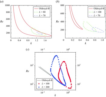
A comparison of neutral curves in the
 $Re{-}k$
plane, corresponding to the centre-mode instability, obtained using the Oldroyd-B and FENE-P models, for (a)
 $\beta = 0.8$
,
 $E = 0.28$
, (b)
 $\beta = 0.8$
,
 $E = 0.42$
, and (c)
 $\beta = 0.9$
,
 $E = 1.05$
(
 $L = 100$
). Finite extensibility has a stabilising effect in (a); in contrast, in (b) and (c), finite extensibility destabilises the centre mode, leading to instability even for
 $k$
values where the Oldroyd-B fluid remains stable.
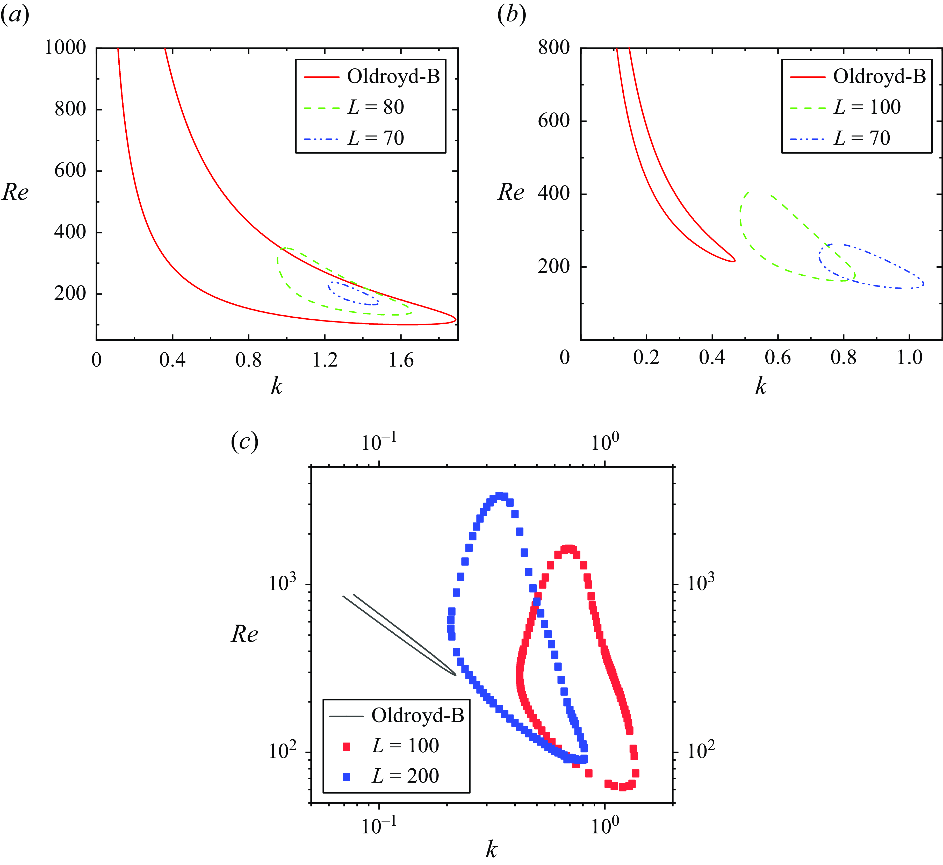
In figure 8, we demonstrate the contrasting effects of decreasing
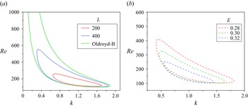
 $L$
, on the neutral tongues in the
 $Re$
–
 $k$
plane present in the Oldroyd-B limit, with a specific focus on the threshold
 $Re$
(
 $Re_c$
, interpreted as the minimum of the neutral islands in the
 $Re$
–
 $k$
plane) required for the centre-mode instability. Figure 8(a) shows the role of decreasing
 $L$
for a relatively small
 $E$
(
 $= 0.28$
): both
 $L = 70$
and
 $L=80$
exhibit a closed unstable loop in the
 $Re$
–
 $k$
plane, for reasons mentioned above. As
 $L$
is decreased from infinity down to
 $70$
,
 $Re_c$
gradually increases, with a concomitant decrease in the size of the island; this trend is largely consistent with the stabilising role of shear thinning, for small
 $E$
, seen earlier in figure 4(a). However, as
 $E$
is increased to
 $0.42$
(figure 8
b), the counterintuitive destabilising role of finite extensibility becomes evident, with
 $Re_c$
for the FENE-P model becoming lower than that in the Oldroyd-B limit. Interestingly, the range of wavenumbers over which the flow is unstable also shifts towards higher values with decreasing
 $L$
. Figure 8(c) illustrates the stronger destabilisation due to finite extensibility at a higher
 $\beta = 0.9$
and
 $E = 1.05$
. Here, in contrast to figures 8(a) and 8(b), the unstable region, while still an island, is significantly larger in its spatial extent than the original Oldroyd-B tongue. The decrease in
 $Re_c$
is also substantial: from
 $Re_c \approx 300$
(for the Oldroyd-B fluid) to
 $Re_c \approx 50$
for
 $L=50$
.
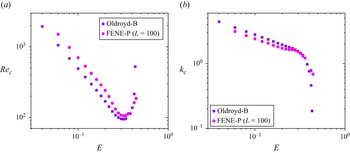
Variation of critical parameters (
 $Re_c$
and
 $k_c$
) with
 $E$
for Oldroyd-B and FENE-P models at
 $\beta = 0.8$
: (a) critical Reynolds number
 $Re_c$
; (b) critical wavenumber
 $k_c$
.
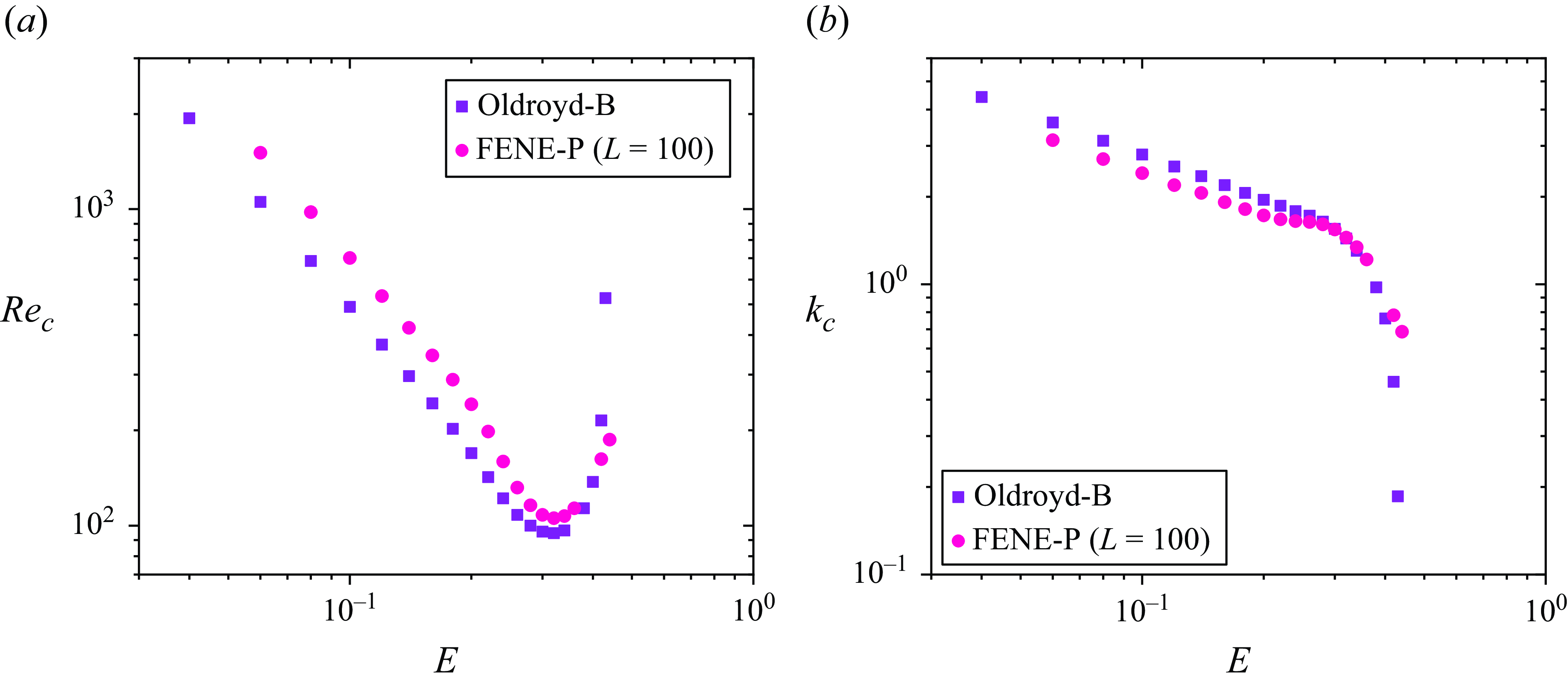
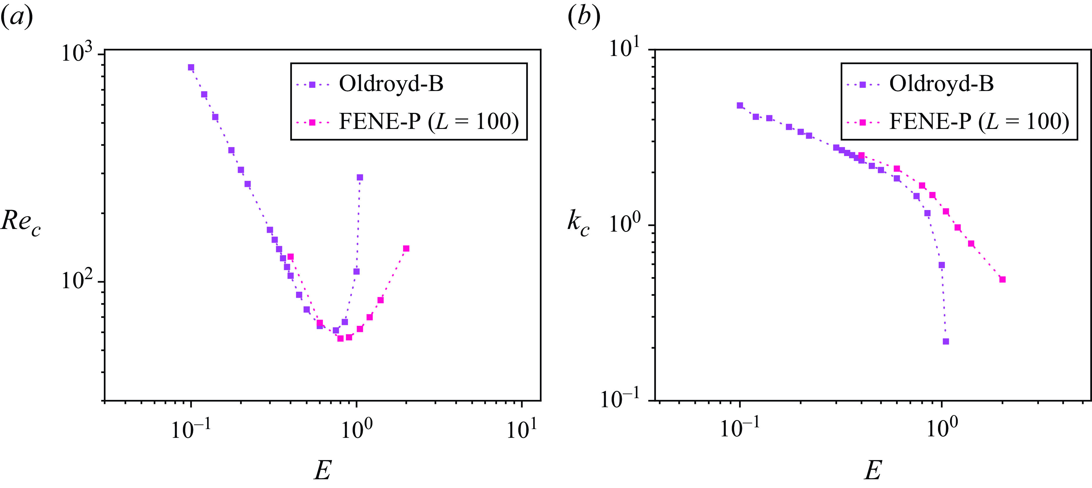
Figures 9(a) and 10(a) show the variation of the critical Reynolds number
 $Re_c$
, and figures 9(b) and 10(b) the corresponding wavenumber
 $k_c$
, with
 $E$
, for a FENE-P fluid with
 $L = 100$
, and for two different values of
 $\beta$
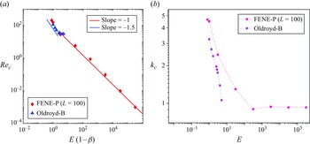
. Results obtained using the Oldroyd-B model are shown for the purposes of comparison. For the lower
 $\beta \ (=0.8)$
, figure 9(a) shows that
 $Re_c \propto E^{-3/2}$
for
 $E \ll 1$
, for both Oldroyd-B and FENE-P fluids, with the only difference being the slightly higher
 $Re_c$
(at a given
 $E$
) for the latter. This slight increase could again be attributed to the expected stabilising role of shear thinning, owing to the higher
 $W$
values along this branch. The
 $E^{-3/2}$
scaling above can be rationalised (Chaudhary et al. Reference Chaudhary, Garg, Subramanian and Shankar2021) using a boundary-layer-type scaling argument that posits that at high
 $Re$
, the disturbance is confined to a thin region near the channel centreline, with elastic, viscous and inertial effects being equally dominant. The
 $Re_c \propto E^{-3/2}$
scaling implies that
 $W_c \propto E^{-1/2}$
for
 $E \ll 1$
; thus at sufficiently small
 $E$
values (i.e.
 $E \lt L^{-2}$
),
 $W_c/L$
will be large enough for the centre mode to be stabilised, and one expects a departure from the
 $E^{-3/2}$
scaling. However, in figure 9(a), for the lowest
 $E$
examined for the FENE-P model (
 $E \sim 0.05$
),
 $W_c \sim 40$
and
 $W/L \sim 0.4$
, implying that the stabilising influence of finite extensibility is not yet significant. It is possible that for the chosen
 $L$
, at sufficiently small
 $E$
values (lower than those examined in figure 9
a), the centre mode is stabilised in the FENE-P model due to shear thinning of
 $\Psi _1$
.
For larger
 $E$
, in figure 9(a),
 $Re_c$
increases sharply, appearing to diverge at a finite
 $E\ (=0.4)$
for the Oldroyd-B case; the increase is more gradual for the FENE-P fluid. Note that the latter increase is on account of the unstable island shifting upward in the
 $Re$
–
 $k$
plane (data not shown), while simultaneously decreasing in size. Given the eventual small size of the shrinking island, it is difficult to determine whether the FENE-P increase is also indicative of a finite-
 $E$
divergence. Nevertheless, as seen in figure 9(a), the instability does appear to be absent for both models at sufficiently high
 $E$
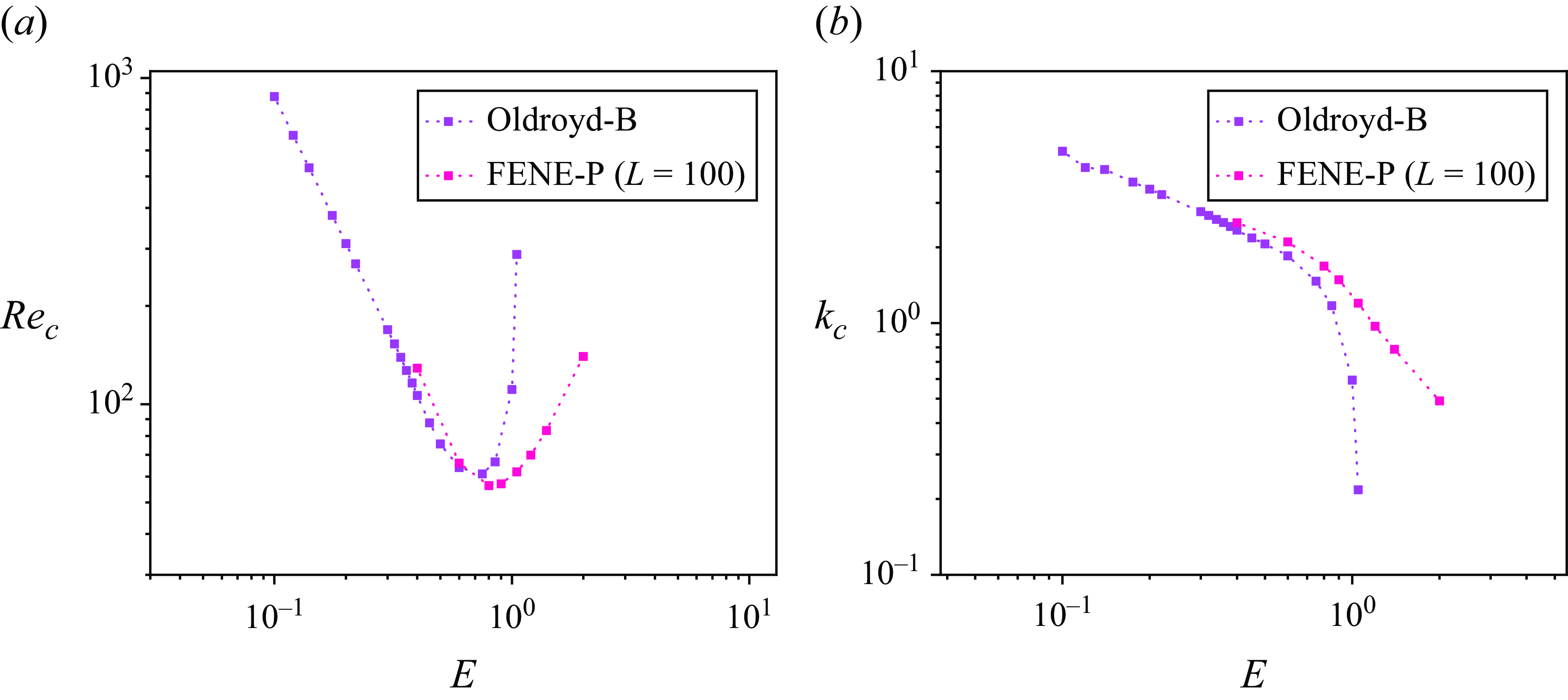
. Figure 10(a) shows a similar trend for
 $\beta = 0.9$
. The divergence of the Oldroyd-B threshold is now postponed until
 $E\approx 1$
, while the increase in
 $Re_c$
for the FENE-P model is more gradual than for
 $\beta = 0.8$
. Figures 9(b) and 10(b) show that the threshold wavenumber mirrors the variation in
 $Re_c$
:
 $k_c$
plummets to zero at a finite
 $E$
for the Oldroyd-B case, while exhibiting a slower decrease for FENE-P, with this decrease being more gradual for
 $\beta = 0.9$
.
Variation of critical parameters (
 $Re_c$
and
 $k_c$
) with
 $E$
for the Oldroyd-B and FENE-P models at
 $\beta = 0.9$
: (a) critical Reynolds number
 $Re_c$
; (b) critical wavenumber
 $k_c$
.
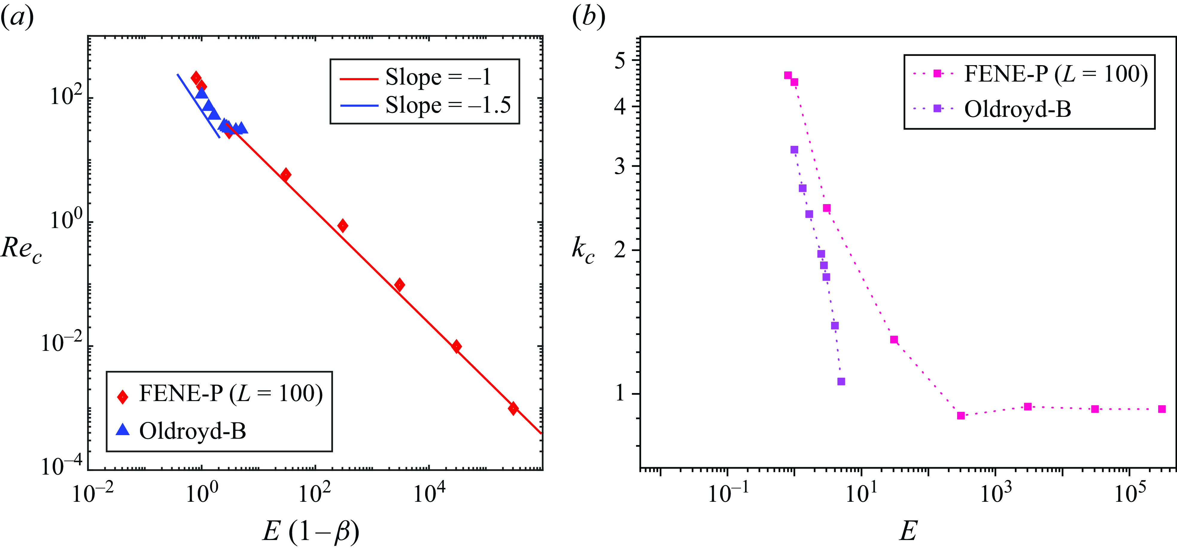
Variation of critical parameters (
 $Re_c$
and
 $k_c$
) with
 $E$
for the Oldroyd-B and FENE-P models at
 $\beta = 0.97$
: (a) critical Reynolds number
 $Re_c$
; (b) critical wavenumber
 $k_c$
. The instability persists in the limit
 $E \rightarrow \infty$
,
 $Re \rightarrow 0$
.
For the Oldroyd-B fluid, the above trend continues until
 $\beta = 0.990552$
, after which there is a continuous decrease of
 $Re_c$
with
 $E$
, all the way up to
 $E \rightarrow \infty$
, implying a smooth crossover from the elastoinertial centre mode to a purely elastic centre-mode instability. Figure 11(a) shows that for a
 $\beta \ (= 0.97)$
lower than the critical value above, while the Oldroyd-B results still show the instability to be absent beyond a threshold
 $E$
, the FENE-P results show a continuation of the elastoinertial centre-mode instability to the elastic one instead. As seen in figure 11(b),
 $k_c$
now remains
 $O(1)$
even as
 $E \rightarrow \infty$
in the FENE-P case. In the next subsection, we proceed to examine in detail this purely elastic centre-mode instability, in FENE-P channel flow, for
 $\beta \geqslant 0.97$
.
3.3.
The elastic centre mode:
 $Re = 0$
(
$E \rightarrow \infty$
)


Elastic spectrum for pressure-driven channel flow of (a) FENE-P (
 $L = 100$
,
 $U_{max} = 1.01254$
) and (b) Oldroyd-B fluids, for
 $\beta = 0.98$
,
 $k = 2$
,
 $W = 200$
. (c,d) Zoomed-in regions of (a) and (b), respectively, near the centre mode (ECM).
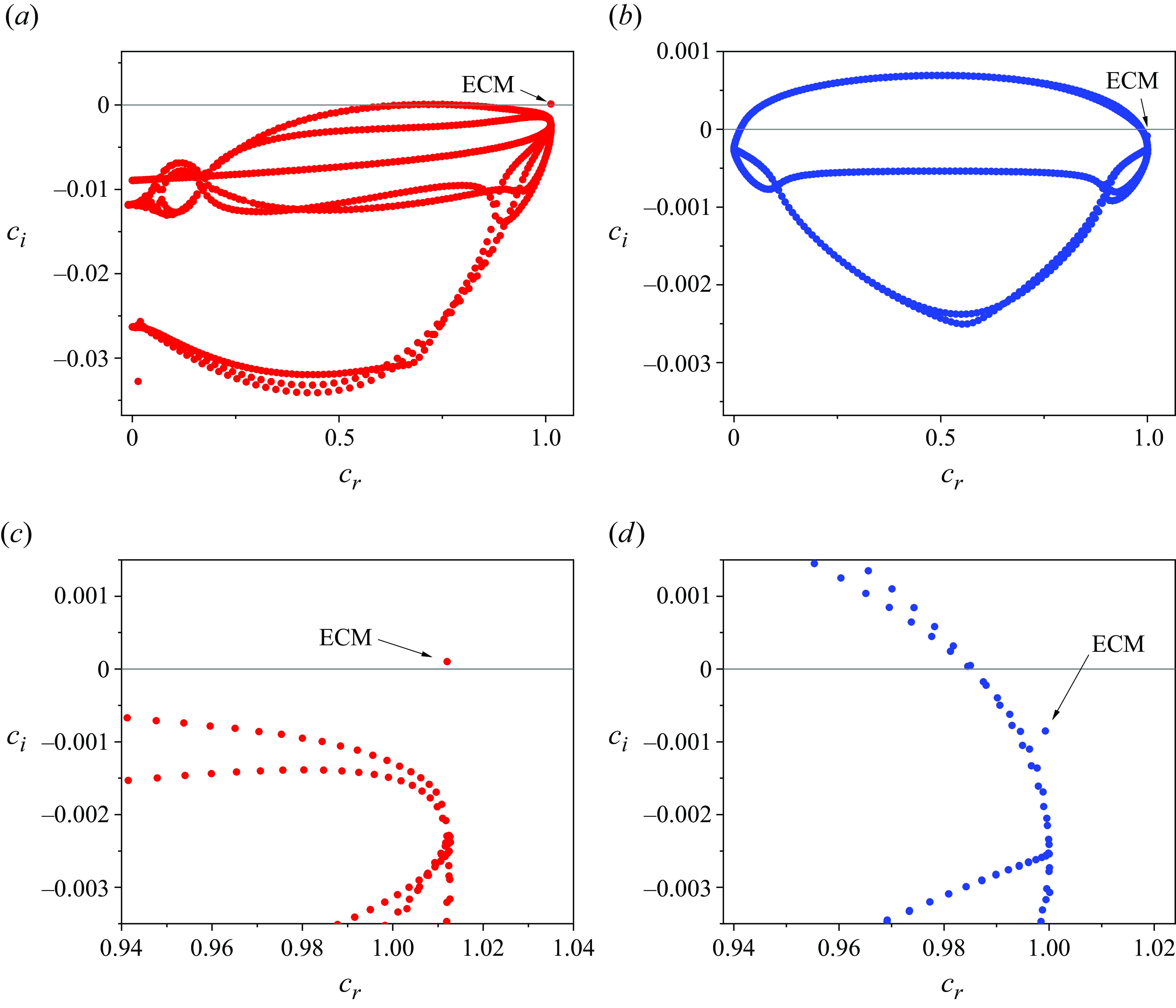
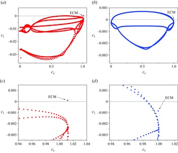
In this subsection, we focus exclusively on the creeping flow limit and examine parameter regimes corresponding to the elastic centre-mode instability, within the framework of the FENE-P model. The elastic spectra for pressure-driven channel flow for
 $\beta = 0.98$
, for both FENE-P and Oldroyd-B fluids, are shown in figures 12(a–d); as for the elastoinertial case in figure 3, figures 12(a) and 12(b) show the overall spectrum, while figures 12(c) and 12(d) focus on the region close to the centre mode. For the chosen
 $\beta$
, the earlier effort by Khalid et al. (Reference Khalid, Shankar and Subramanian2021b
) has shown that the centre mode is stable for the Oldroyd-B fluid (the unstable interval being
 $0.990552 \lt \beta \lt 1$
). In contrast, the elastic spectrum for the FENE-P fluid shows an unstable centre mode, as expected from the results shown in figure 11(a) in § 3.2; this also reinforces the trend of finite-extensibility-induced destabilisation at higher (but finite)
 $E$
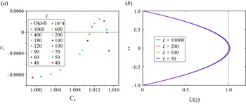
values already found in § 3.1. This trend is explored more systematically in figure 13(a), wherein the elastic centre mode is tracked as
 $L$
is decreased from the Oldroyd-B limit (
 $L = \infty$
) down to
 $L = 40$
, again for
 $\beta = 0.98$
. The centre mode is unstable for
 $45 \lt L \lt 110$
, corresponding to
 $0.225 \lt W/L \lt 0.55$
. Figure 13(b) shows that in contrast to the sensitive change in the stability characteristics, there is little variation in the base-flow velocity profiles over the said range of
 $L$
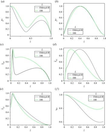
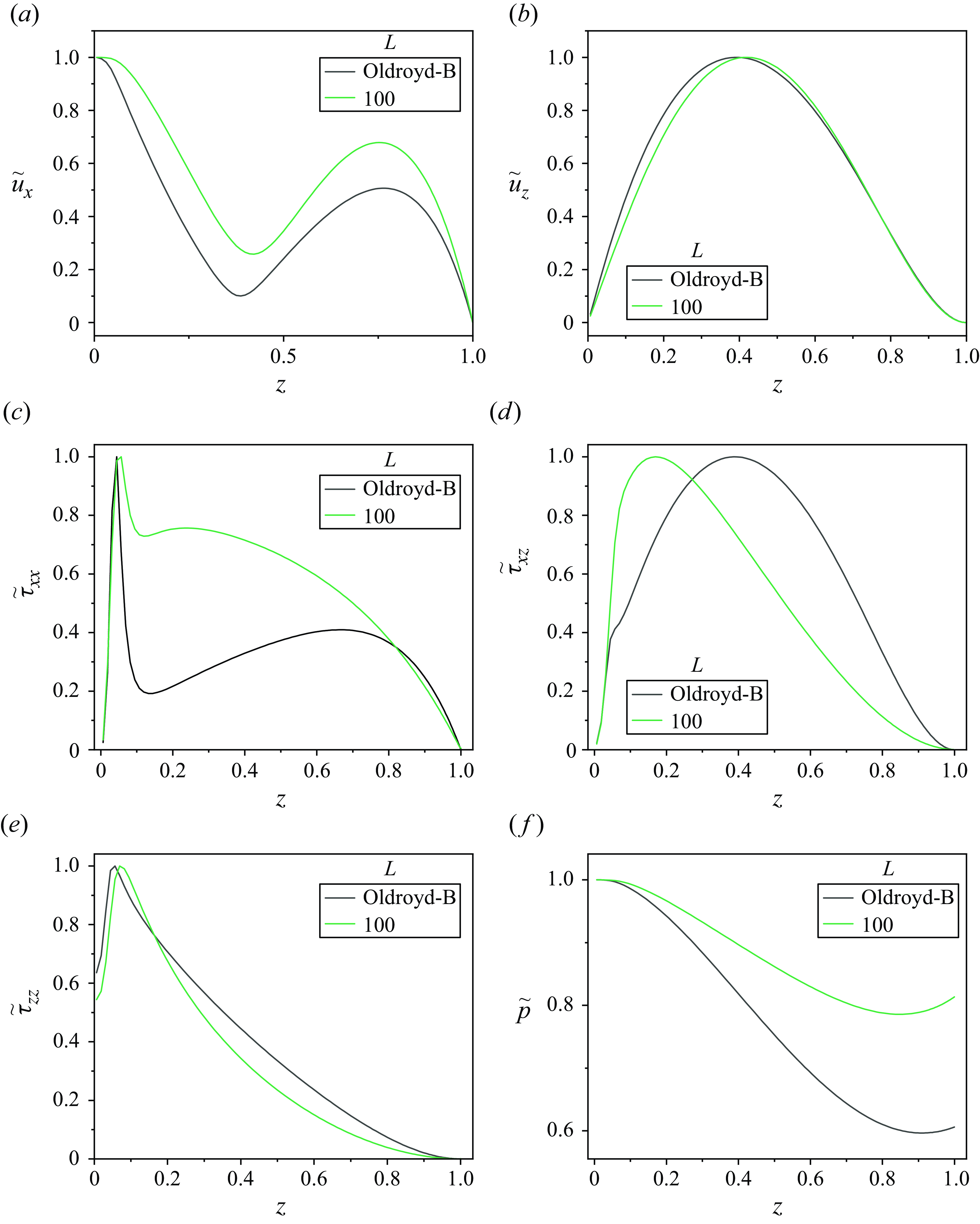
values. The velocity and stress eigenfunctions for the Oldroyd-B and FENE-P cases are shown in figure 14. Similar to the elastoinertial case discussed earlier (figure 5), one finds the velocity eigenfunctions to be qualitatively similar for both FENE-P and Oldroyd-B fluids, with significant differences discernible only in the
 $\tilde {\tau }_{xx}$
and
 $\tilde {\tau }_{xz}$
eigenfunctions, and with differences in the former being more pronounced.
(a) Elastic spectra: the enlarged spectrum (near the centre mode) showing the variation in the centre mode as
 $L$
is varied at
 $\beta = 0.98$
,
 $k = 2$
,
 $W=200$
and
 $Re = 0$
. (b) The base flow velocity profiles for the same
 $\beta$
and
 $W$
, and for different
 $L$
values.
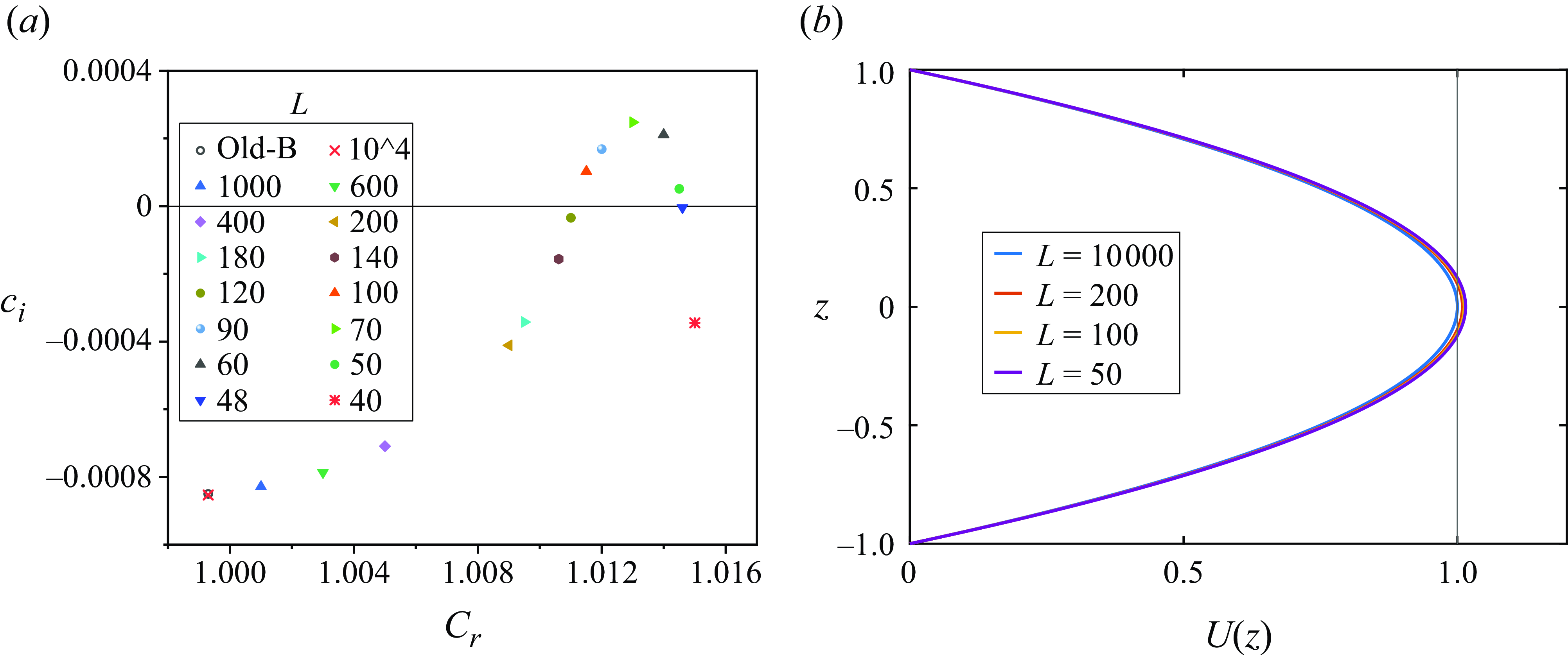
Velocity, stress and pressure eigenfunctions corresponding to the elastic centre mode in figure 13 for
 $\beta = 0.98$
,
 $k = 2$
and
 $W=200$
, in the Oldroyd-B limit and for
 $L=100$
. The corresponding eigenvalues are:
 $L = 100$
(
 $U_{max} = 1.01254$
),
 $c = 1.0120157 + 0.000102{\rm i}$
; Oldroyd-B (
 $U_{max} = 1$
),
 $c = 0.999277 - 0.000850{\rm i}$
.
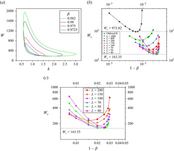
The elastic centre-mode instability within the FENE-P framework. (a) The neutral curves in the
 $W$
–
 $k$
plane for different
 $\beta$
values for
 $L = 100$
. (b) The variation of the critical Weissenberg number
 $W_c$
with
 $(1-\beta )$
for different
 $L$
values. (c) An expanded view of the region of (b) for
 $40 \leqslant L \leqslant 200$
.
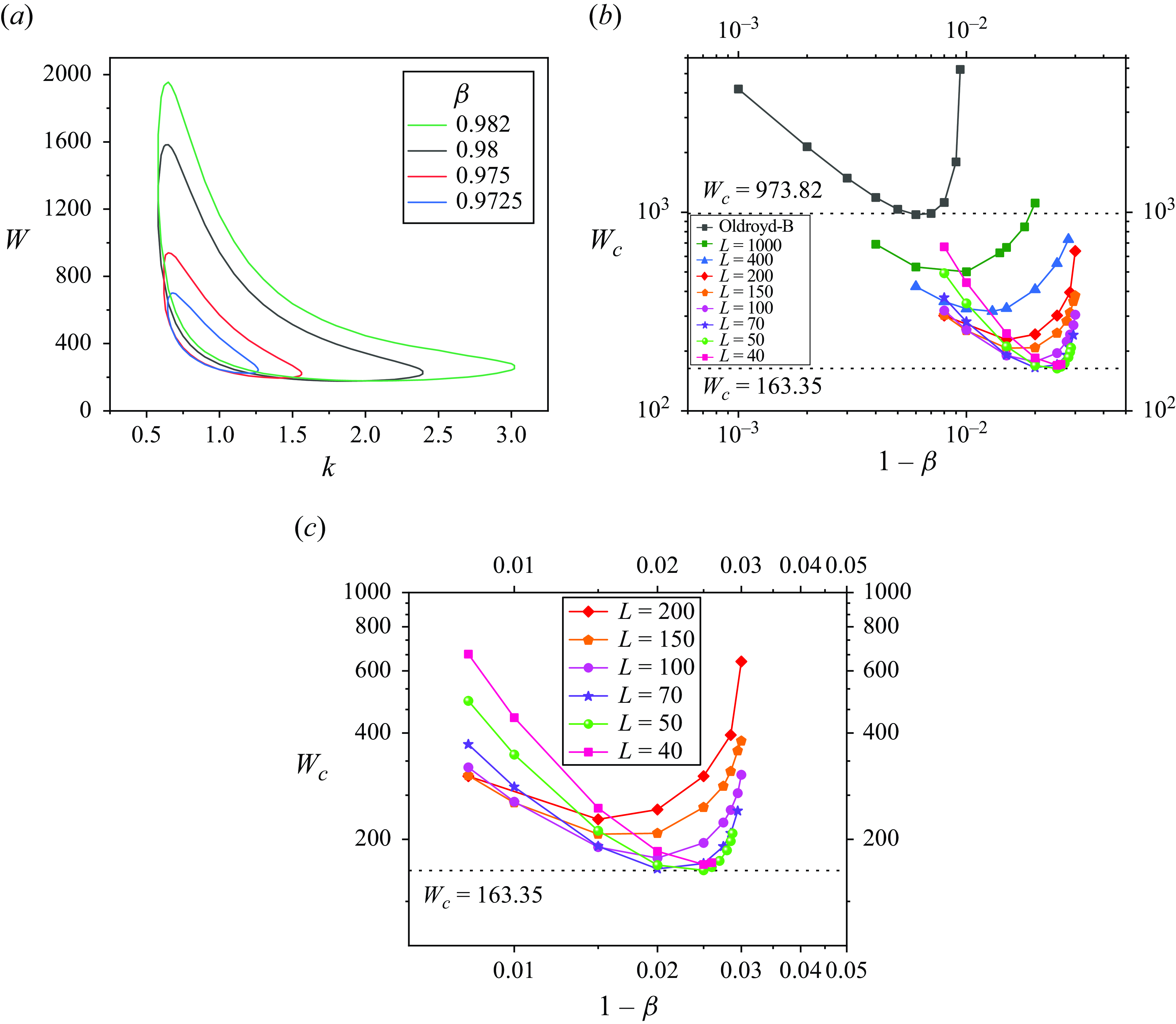
The neutral curves for the elastic centre-mode instability, in the
 $W$
–
 $k$
plane, are shown for different
 $\beta$
values (for
 $L = 100$
) in figure 15(a). Similar to the
 $Re$
–
 $k$
neutral curves for the elastoinertial instability discussed earlier, unstable regions take the form of islands, but now in the
 $W$
–
 $k$
plane. The reason for the island, as opposed to the tongue for the Oldroyd-B case (see Khalid et al. Reference Khalid, Shankar and Subramanian2021b
), is again the same as in the elastoinertial case – shear thinning. The variation of the critical Weissenberg number
 $W_c$
(minima of the neutral curves in the
 $W$
–
 $k$
plane) with
 $(1-\beta )$
is shown for different
 $L$
values in figure 15(b), along with the result obtained earlier using the Oldroyd-B model by Khalid et al. (Reference Khalid, Shankar and Subramanian2021b
). There is a systematic decrease of
 $W_c$
with decreasing
 $L$
, with the critical
 $W_c$
required for instability coming down to
 $W_c \lt 200$
for
 $L \approx 100$
; eventually, for small enough
 $L\ (\lesssim 40)$
, the
 $W_c$
curve starts to move up again, as evident from the magnified view in figure 15(c). The lowest critical value
 $W_c \approx 163$
for
 $\beta = 0.975$
is consistent with the value reported in the study of Buza et al. (Reference Buza, Page and Kerswell2022). Both figures 15(a) and 15(b) also serve to show that the elastic instability exists over a wider range of
 $\beta$
(
 $0.97 \lesssim \beta \lt 1$
), compared to the Oldroyd-B model (
 $0.990552 \leqslant \beta \lt 1$
). In both cases,
 $W_c$
eventually increases for
 $\beta$
sufficiently close to unity, owing to the absence of the elastic instability in the Newtonian limit (
 $\beta = 1$
).
4. Role of finite extensibility using the FENE-CR model
The role of finite polymer extensibility, as modelled using the FENE-CR constituive equation, is explored next. As mentioned in the Introduction, a key difference between the FENE-P and FENE-CR models is the lack of shear thinning of viscosity in the latter, which results in a parabolic base-state velocity profile (similar to the Newtonian or Oldroyd-B cases); thus, unlike the FENE-P case, the (non-dimensional) base-state maximum always equals unity. The first normal stress coefficient does exhibit a shear thinning behaviour, although it scales differently with
 $W$
for
 $W \gg 1$
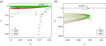
compared to the FENE-P fluid. The elastoinertial spectra for channel flow of a FENE-CR fluid, for the same set of parameters as figure 3, namely
 $Re = 800$
,
 $E = 0.1$
,
 $k=1.5$
and
 $\beta = 0.8$
, are shown in figure 16 for
 $L = 100$
and
 $200$
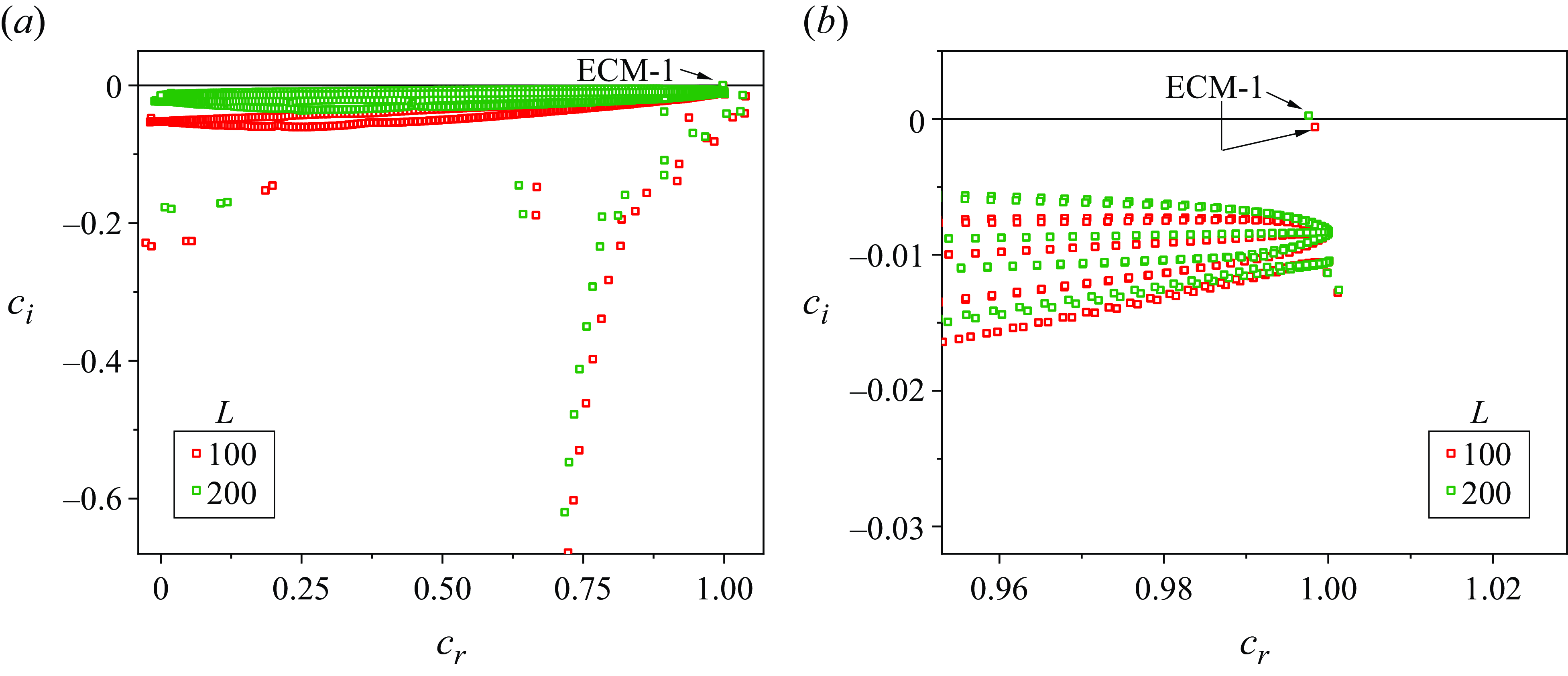
. While there exists an unstable centre mode for
 $L= 200$
, it is stabilised for
 $L = 100$
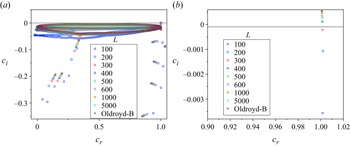
. Figure 17 shows (for a lower
 $Re = 150$
) that there is a monotonic stabilisation of the centre mode as
 $L$
is decreased from the Oldroyd-B limit (
 $L = \infty$
) down to
 $L = 100$
, with
 $c_i$
crossing zero at
 $L \approx 350$
. The real part of the phase speed
 $c_r$
is much closer to unity in all cases examined, on account of the base velocity profile for the FENE-CR fluid being identical to its Oldroyd-B counterpart.
Elastoinertial spectrum obtained using the FENE-CR model for
 $Re = 800$
,
 $E = 0.1$
,
 $\beta = 0.8$
,
 $k = 1.5$
for two
 $L$
values: (a) the full spectrum; (b) enlarged view of (a) near the unstable centre mode.
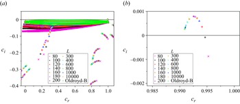
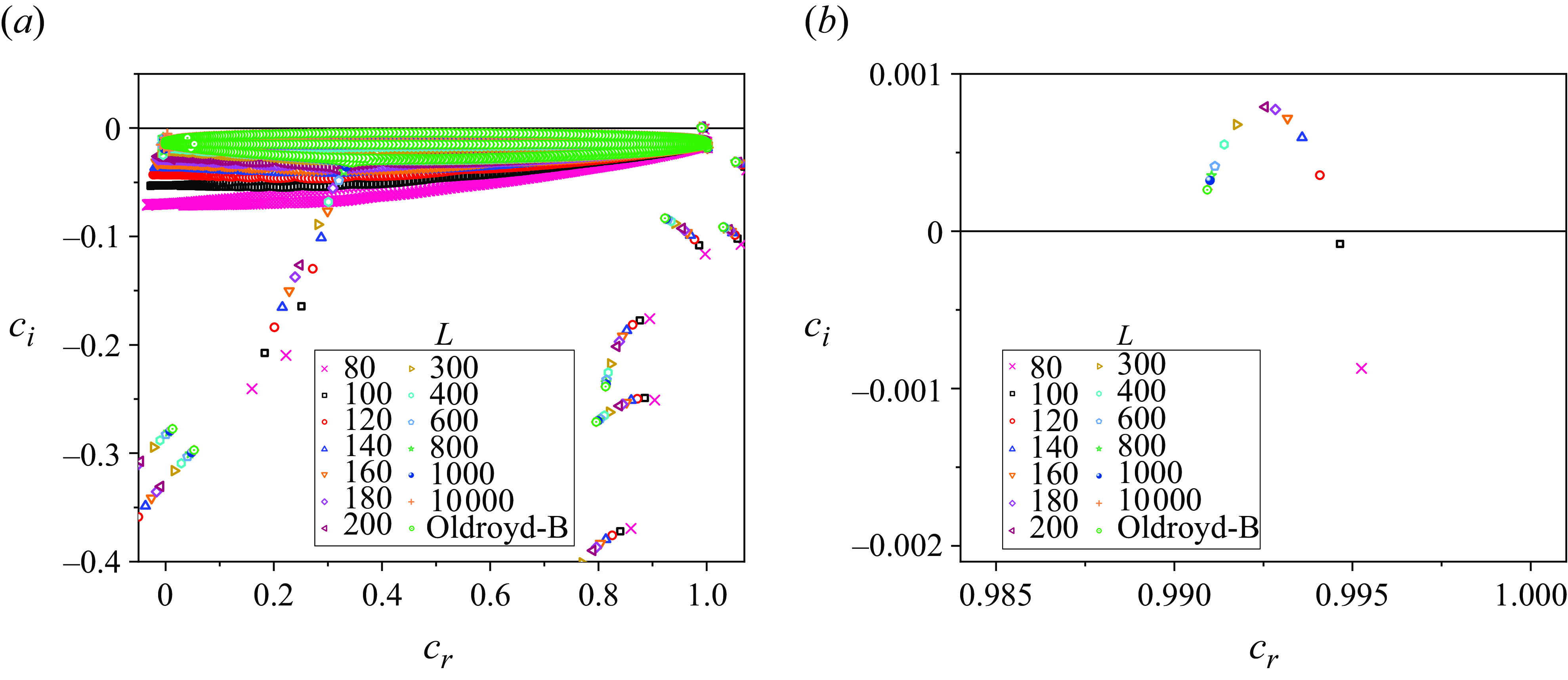
We carried out a comprehensive search of the parameter space, in order to examine whether the FENE-CR model can render the centre mode unstable, in a manner similar to the FENE-P case. For the vast majority of parameter combinations, finite extensibility within the FENE-CR model always resulted in stabilisation, with
 $c_i$
decreasing monotonically with decreasing
 $L$
, similar to figure 16(b). However, we did find occasional deviations from this trend, an example of which is shown in figure 18. Here, the unstable centre mode in the Oldroyd-B model is further destabilised by finite extensibility to begin with, the centre mode eventually becoming stable for
 $L \lt 100$
. As will be seen in figures below, such deviations did not affect the threshold values. It is also important to note that, unlike the FENE-P case, we did not find an unstable centre mode within the FENE-CR framework for parameter regimes where it is stable in the Oldroyd-B limit.
Elastoinertial spectrum obtained using the FENE-CR model for
 $\beta=0.8$
,
 $Re=150$
,
 $k=1.5$
,
 $E=0.3$
for
 $L$
ranging from
 $\infty$
down to
 $100$
. (a) The complete elastoinertial spectrum. (b) Zoomed-in view of (a) near the ECM. The unstable centre mode in the Oldroyd-B model becomes stable for
 $L \lesssim 300$
.
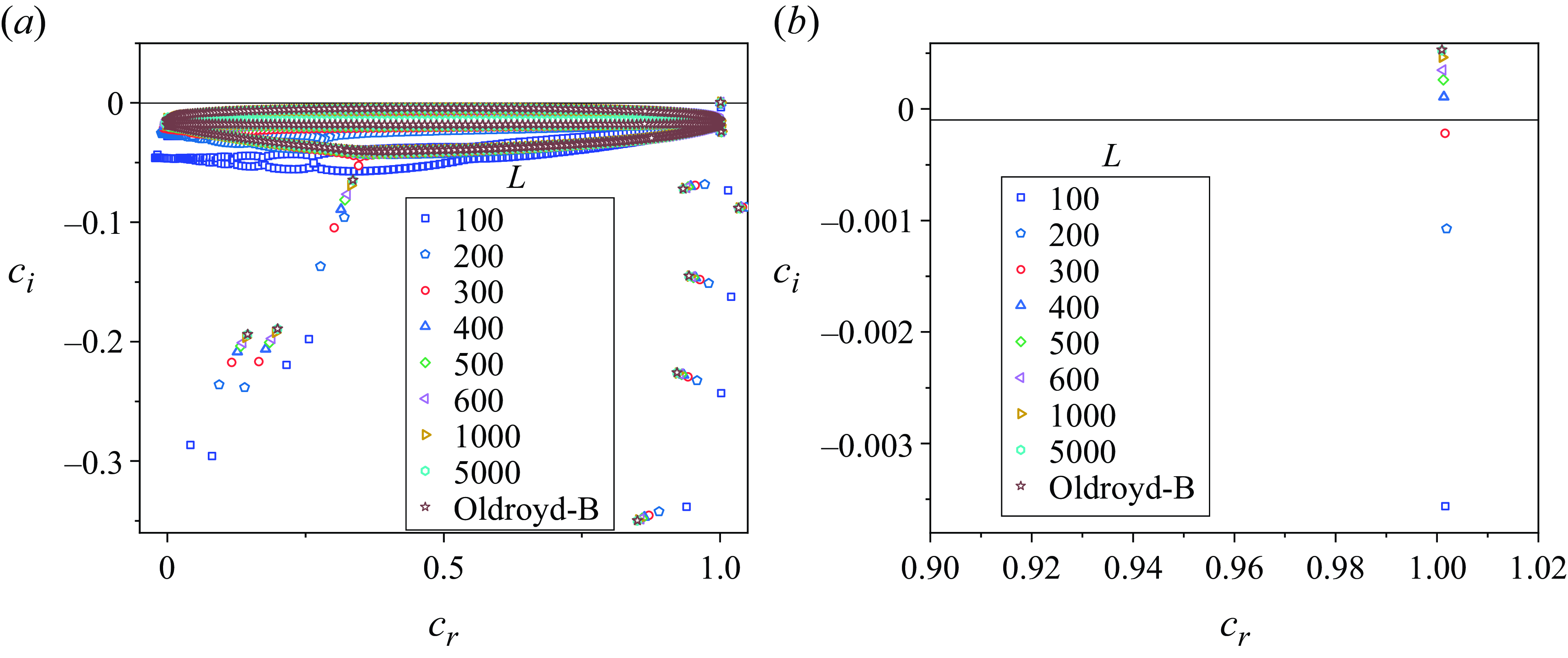
Elastoinertial spectrum obtained using the FENE-CR model for
 $Re = 150$
,
 $E = 0.4$
,
 $\beta = 0.9$
,
 $k = 1.25$
for
 $L$
ranging from
 $\infty$
down to
 $80$
. (a) The full spectrum. (b) Enlarged view of (a) near the centre mode.
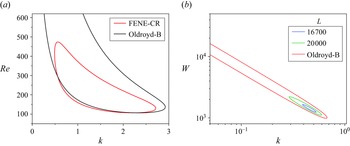
The neutral stability curves in the
 $Re$
–
 $k$
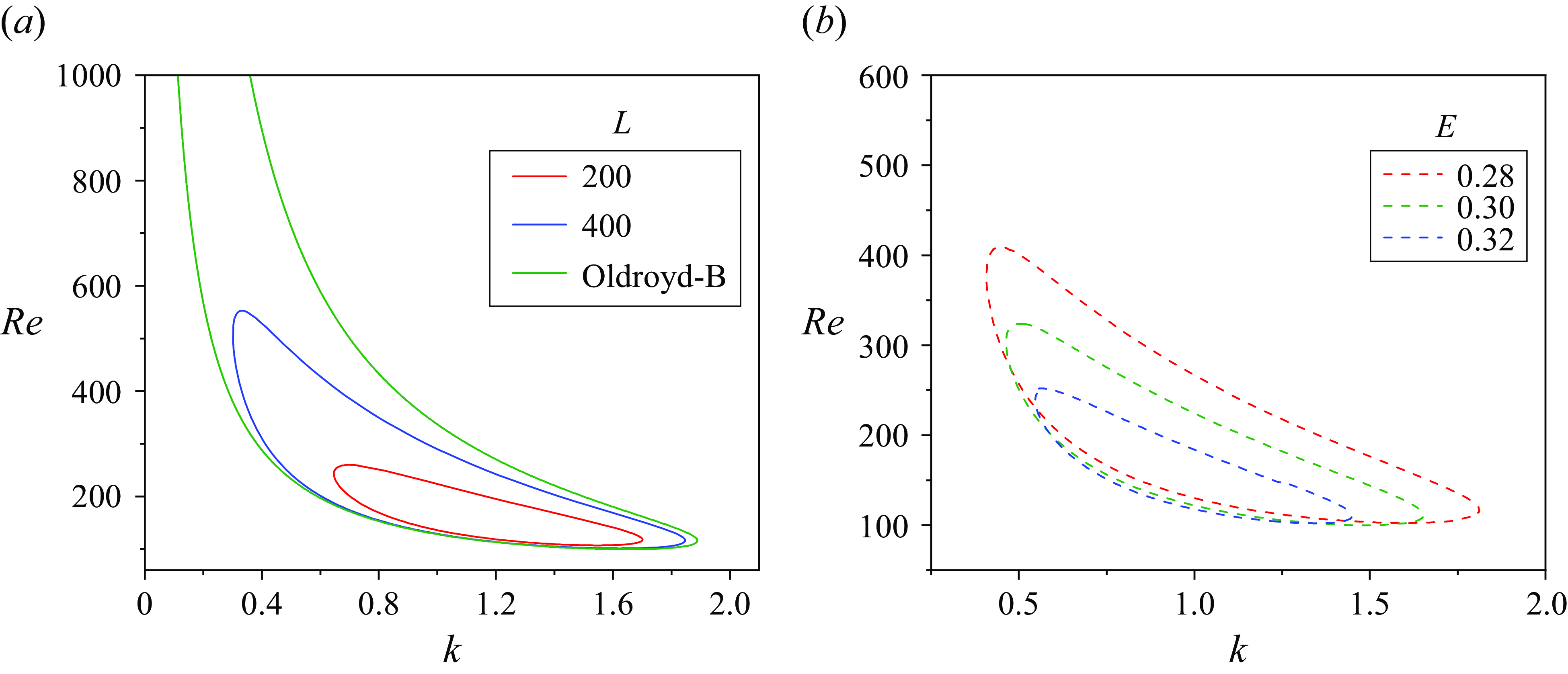
plane, shown in figure 19(a), are generally consistent with the trend of monotonic stabilisation with decreasing
 $L$
. The unstable regions in the
 $Re$
–
 $k$
plane are islands, similar to the FENE-P results discussed earlier (the underlying reason being the shear thinning of
 $\Psi _1$
). Unlike in the FENE-P case, the size of the unstable island shrinks as
 $L$
is decreased. The effect of varying
 $E$
at a fixed
 $L\ (= 300)$
is shown in figure 19(b), where the size of the unstable island again decreases monotonically with increasing
 $E$
, with the unstable
 $k$
-interval at higher
 $E$
values being a subset of those at lower
 $E$
values. In figure 20(a), the slight destabilising role of decreasing
 $L$
is evident for
 $0.5 \lt k \lt 1.5$
, wherein the FENE-CR island lies somewhat below the Oldroyd-B tongue. However, both models predict nearly identical
 $Re_c$
, thereby making the slight destabilisation for
 $k \lt k_c$
(i.e. for
 $k \approx 1$
) inconsequential from an experimental standpoint.
Neutral stability curves in the
 $Re$
–
 $k$
plane obtained using the FENE-CR model for
 $\beta = 0.8$
: (a)
 $E = 0.28$
for different
 $L$
values; (b)
 $L = 300$
for different
 $E$
values.
(a) Neutral stability curves in the
 $Re$
–
 $k$
plane obtained using the FENE-CR and Oldroyd-B models: data for
 $\beta =0.8$
,
 $E = 0.4$
and
 $L = 200$
. (b) The FENE-CR neutral stability curves in the
 $W$
–
 $k$
plane for different
 $L$
values, in the creeping flow limit (
 $Re = 0$
) for
 $\beta =0.993$
.
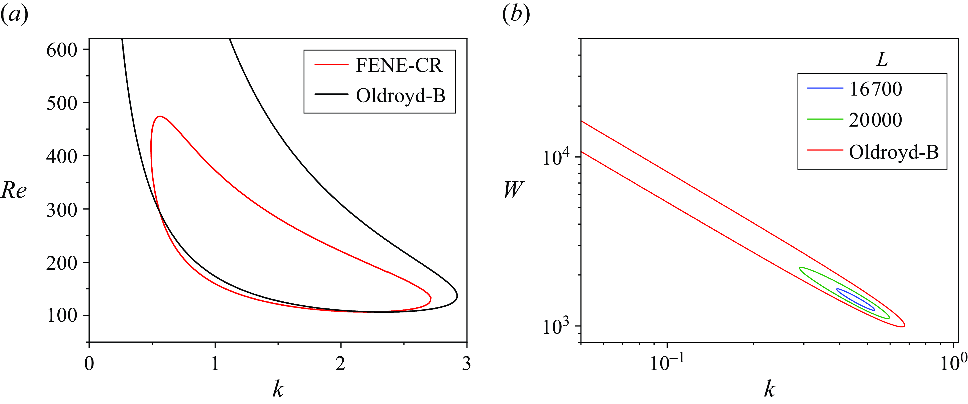
Finally, in figure 20(b), we examine the role of finite extensibility on the elastic centre-mode instability. Mirroring the trend for finite
 $Re$
above, decreasing
 $L$
rapidly stabilises the elastic instability. The unstable tongue in the Oldroyd-B limit transforms to an island for finite
 $L$
, but all of the islands are contained within the original Oldroyd-B tongue, and shrink rapidly with decreasing
 $L$
. For
 $\beta = 0.993$
in figure 20(b), the elastic instability is already absent for
 $L \approx 10^4$
and lower. Since shear thinning of the viscosity is absent for FENE-CR, and negligibly small for FENE-P for
 $\beta = 0.993$
(the ratio of the solvent to solution viscosity decreases from unity to
 $0.993$
, as
 $W$
increases from
 $0$
to infinity), it is the shear-rate dependence of
 $\Psi _1$
that ought to dictate the behaviour of the centre-mode instability at high
 $W$
. As mentioned in the Introduction, the shear thinning of
 $\Psi _1$
is stronger for FENE-P (
 $\Psi _1 \propto W^{-4/3}$
) compared to FENE-CR (
 $\Psi _1 \propto W^{-1}$
), suggesting that the finite-extensibility-induced stabilisation ought to be stronger for the FENE-P fluid. In contrast to this expectation, our results above show that it is the FENE-CR fluid that shows a more rapid stabilisation with a decrease in
 $L$
, this effect being most prominent in the inertialess limit.
5. Concluding remarks
The role of finite extensibility of the polymer molecule on the centre-mode instability in viscoelastic channel flow is examined using the FENE-P and FENE-CR models. The original elastoinertial centre-mode instability is predicted, within the Oldroyd-B framework, for
 $W \sim O(10)$
and higher, with
 $W$
increasing to
 $O(10^3)$
in the creeping flow limit. However, at such high
 $W$
, polymer solutions exhibit shear thinning, leading to a decrease in shear viscosity as well as the first normal stress coefficient with
 $W$
. The latter implies a weakening of elastic effects at higher
 $W$
values, and the effective Weissenberg number
 $W_{eff} = N_1/(2 \tau _{xz})$
actually decreases for the FENE-P model, while plateauing for the FENE-CR model, for
 $W \gg 1$
. Thus, intuitively, finite extensibility is expected to play a stabilising role, and this is generally borne out by our results for the FENE-CR model, and for the FENE-P model at relatively low
 $E$
. However, at higher
 $E$
values, finite extensibility destabilises the centre mode, for
 $L \sim O(100)$
in the FENE-P model, there being unstable centre modes even in parameter regimes where the Oldroyd-B analysis predicts stability. This counterintuitive prediction is consistent with the earlier results of Buza et al. (Reference Buza, Page and Kerswell2022).
We have provided a comprehensive account of the parameter regimes in which the centre-mode instability is expected to occur in viscoelastic channel flow. Notably, for
 $Re \rightarrow 0$
, the elastic centre-mode instability occurs over a wider range of
 $\beta$
values (
 $0.97 \lt \beta \lt 1$
), and at significantly lower
 $W$
values (
 $\sim 100$
) for the FENE-P model with
 $L \sim O(100)$
, thus making experimental observations feasible, especially ones that probe flows of dilute polymer solutions. Nevertheless, our findings with regard to the effects of finite extensibility are counter intuitive. In the dilute regime (
 $\beta \rightarrow 1$
), on account of shear thinning in the FENE-P model, the (dimensionless) total viscosity of the solution varies between
 $1$
(for
 $W \lt L$
) and
 $\beta$
(for
 $W \gt L$
), thus rendering the shear thinning of viscosity negligible – the base flow velocity profiles are indeed very close to the parabolic profile of an Oldroyd-B fluid. As a result, one might anticipate the shear-rate dependence of the first normal stress difference, in the base state, as being a relevant factor underlying this instability. However, this expectation is not borne out by the FENE-CR model, which also has a constant (shear-rate-independent) viscosity, and a shear-rate-dependent
 $\Psi _1$
, albeit with a different exponent (compared to the FENE-P model) characterising shear thinning at high
 $W$
values. Our results show that the latter feature does not generally result in destabilisation of the centre mode within the FENE-CR model. This suggests that decoding the destabilising role of finite extensiblity in the FENE-P model is rather subtle, and requires a more detailed analysis. On the whole, the present effort shows that the use of the more accurate FENE-P model results in viscoelastic channel flow becoming unstable over larger regions of the
 $Re$
–
 $E$
–
 $\beta$
space, and for experimentally relevant values of the extensibility parameter
 $L$
, thereby making the realisation of the centre-mode instability more feasible.
Acknowledgements
The authors thank Dr G. Buza, Dr J. Page and Professor R. Kerswell for providing their data for benchmarking our numerical scheme for the FENE-P fluid.
Declaration of interests
The authors report no conflict of interest.
Author contributions
V.S. and G.S. proposed and designed the research. M.K., A.B., D.D., P.N. and V.S. derived the equations and developed the code. M.K., A.B., D.D. and P.N. performed the simulations. All authors contributed equally to analysing data and reaching conclusions. V.S. and G.S. wrote the paper.
Appendix A. Linearised equations for the FENE-P model
The linearised continuity, momentum (
 $x$
- and
 $z$
-components) equations, and constitutive equations for the FENE-P model are given in this appendix. Below,
 $ {\rm d}_z= {\rm d}/{\rm d}z$
and primes on the base-state profiles represent the derivative with respect to
 $ z$
:
 \begin{equation} {\rm d}_z \tilde {v}+{\rm i} k\tilde {u}=0, \end{equation}
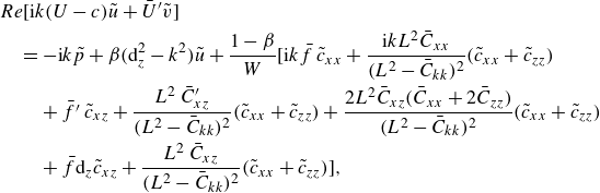 \begin{align} &{}Re\big [ \textrm{i} k (U-c)\tilde {u}+\bar {U}^{\prime}\tilde {v}\big ] \nonumber\\& \quad= -\textrm{i} k \tilde {p}+\beta (\textrm{d}_z^2-k^2)\tilde {u} +\frac {1-\beta }{W} \Bigg [\textrm{i}k \bar {f} \,\tilde {c}_{xx}+\frac {\textrm{i}kL^2\bar {C}_{xx}} {(L^2-\bar {C}_{kk})^2}\big (\tilde {c}_{xx}+\tilde {c}_{zz}\big ) \nonumber \\ &\qquad {}+ \bar {f^{\prime}} \,\tilde {c}_{xz} + \frac {L^2 \, \bar {C}^{\prime}_{xz}}{(L^2-\bar {C}_{kk})^2}(\tilde {c}_{xx} +\tilde {c}_{zz}) + \frac {2L^2\bar {C}_{xz} (\bar {C}_{xx}+2\bar {C}_{zz})}{(L^2-\bar {C}_{kk})^2}(\tilde {c}_{xx}+\tilde {c}_{zz})\nonumber \\ &\qquad{}+\bar {f}\textrm{d}_z\tilde {c}_{xz}+ \frac {L^2 \, \bar {C}_{xz}}{(L^2-\bar {C}_{kk})^2}(\tilde {c}_{xx}+\tilde {c}_{zz})\Bigg ], \end{align}
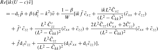 \begin{align} & Re \big [\textrm{i}k(U-c)\tilde {v}\big ]\nonumber\\ &\quad = -{\textrm{d}_z}\tilde {p}+\beta (\textrm{d}_z^2-k^2)\tilde {v}+\frac {1-\beta }{W} \Bigg [\textrm{i}k \bar {f} \,\tilde {c}_{xz} +\frac {\textrm{i}kL^2\bar {C}_{xz}} {(L^2-\bar {C}_{kk})^2}(\tilde {c}_{xx}+\tilde {c}_{zz})\nonumber\\ &\qquad{}+ \bar {f^{\prime}} \,\tilde {c}_{zz}+ \frac {L^2 \, \bar {C}^{\prime}_{zz}}{(L^2-\bar {C}_{kk})^2}(\tilde {c}_{xx} +\tilde {c}_{zz}) + \frac {2L^2\bar {C}_{zz} (\bar {C}^{\prime}_{xx}+2\bar {C}^{\prime}_{zz})}{(L^2-\bar {C}_{kk})^2}(\tilde {c}_{xx}+\tilde {c}_{zz})\nonumber\\ &\qquad {}+\bar {f}\textrm{d}_z\tilde {c}_{zz} +\frac {L^2 \bar {C}_{zz}}{(L^2-\bar {C}_{kk})^2}(\textrm{d}_z\tilde {c}_{xx}+\textrm{d}_z\tilde {c}_{zz})\Bigg ], \end{align}
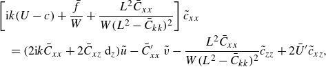 \begin{align} &\left [\textrm{i}k(U-c) +\frac {\bar {f}}{W}+\frac {L^2 \bar {C}_{xx}}{W(L^2 -\bar {C}_{kk})^2}\right ]\tilde {c}_{xx}\nonumber \\ &\quad =(2\textrm{i}k\bar {C}_{xx} +2\bar {C}_{xz} \,\textrm{d}_z)\tilde {u}-\bar {C}^{\prime}_{xx} \, \tilde {v}-\frac {L^2 \bar {C}_{xx}}{W(L^2 -\bar {C}_{kk})^2}\tilde {c}_{zz} +2\bar {U}^{\prime}\tilde {c}_{xz}, \end{align}
 \begin{align} &\left [\textrm{i}k(U-c)+\frac {\bar {f}}{W}\right ]\tilde {c}_{xz}\nonumber \\ &\quad =(\textrm{i}k\bar {C}_{xz}+\bar {C}_{zz} \, \textrm{d}_z) \tilde {u} -\frac {L^2 \bar {C}_{xz}}{W(L^2 -\bar {C}_{kk})^2} (\tilde {c}_{xx} +\tilde {c}_{zz} )-(\bar {C}^{\prime}_{xz} \, - \textrm{i} k \bar {C}_{xx} - \bar {C}_{xz}\, \textrm{d}_z) \tilde {v}, \end{align}
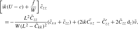 \begin{align} &\left [\textrm{i}k(U-c)+\frac {\bar {f}}{W}\right ]\tilde {c}_{zz}\nonumber \\ &\quad = -\frac {L^2 \bar {C}_{zz}}{W(L^2 -\bar {C}_{kk})^2}\big (\tilde {c}_{xx}+\tilde {c}_{zz}\big )+(2\textrm{i}k\bar {C_{xz}} \, - \bar {C}^{\prime}_{zz} + 2\bar {C}_{zz}\, \textrm{d}_z) \tilde {v}, \end{align}
 \begin{align} &\left [\textrm{i}k(U-c)+\frac {\bar {f}}{W}\right ]\tilde {c}_{yy}= {} -\frac {L^2 \bar {C}_{yy}}{W(L^2 -\bar {C}_{kk})^2}\big (\tilde {c}_{xx}+\tilde {c}_{yy}+\tilde {c}_{zz}\big ) - \bar {C}^{\prime}_{zz} \tilde {v}. \end{align}
Appendix B. Linearised governing equations for the FENE-CR model
This appendix contains the linearised governing equations and constitutive relations for the FENE-CR model:
 \begin{equation} \textrm{i}k\tilde {u} + \textrm{d}_z\tilde {v} = 0, \end{equation}
 \begin{equation} [\textrm{i}k\,Re\,(U - c) - \beta (\textrm{d}_z^2 - k^2)]\tilde {u}= -\textrm{i}k\tilde {p} -Re\, U^{\prime} \tilde {v} + [\textrm{i}k\hat {\tau }_{xx} + \textrm{d}_z\tilde {\tau }_{xz}], \end{equation}
 \begin{equation} [\textrm{i}k\,Re\,(U - c) - \beta (\textrm{d}_z^2 - k^2)]\tilde {v}= -\textrm{d}_z\hat {p} + [\textrm{i}k\tilde {\tau }_{xz} + \textrm{d}_z\tilde {\tau }_{zz}], \end{equation}
 \begin{equation} [\textrm{i}k(U - c)]\tilde {c}_{xx} = 2(\textrm{i}k\overline {C}_{xx} + \overline {C}_{xz}D)\tilde {u} -\tilde {v} \overline {C}_{xx}^{\prime} + 2 U^{\prime} \tilde {c}_{xz} - \frac {\tilde {\tau }_{xx}}{1-\beta }, \end{equation}
 \begin{equation} [\textrm{i}k(U - c)]\tilde {c}_{xz} = \overline {C}_{zz} \textrm{d}_z \tilde {u} + (\textrm{i}k\overline {C}_{xx} + \overline {C}_{xz}^{\prime} )\tilde {v} + U^{\prime} \tilde {c}_{zz} - \frac {\tilde {\tau }_{xz}}{1-\beta }, \end{equation}
 \begin{equation} [\textrm{i}k(U - c)]\tilde {c}_{zz} = (2\textrm{i}k\overline {C}_{xz} + 2\overline {C}_{zz}\textrm{d}_z - \overline {C}_{zz}^{\prime} )\tilde {v}_z - \frac {\tilde {\tau }_{zz}}{1-\beta }, \end{equation}
 \begin{equation} [\textrm{i}k(U - c)]\tilde {c}_{yy} = - \overline {C}_{zz}^{\prime} \tilde {v}_z - \frac {\tilde {\tau }_{yy}}{1-\beta }, \end{equation}
where
 ${\rm d}_z = {\rm d}/{\rm d}z$
, as before. Next, we express the stress eigenfunctions in terms of the eigenfunctions of the conformation tensor. The conformation tensor and stress tensor are related by (2.4). This equation also contains the Peterlin function
 $f$
, which, in turn, is a function of the trace of the conformation tensor. A binomial expansion can be used to express, within linear order, the Fourier mode coefficient
 $\tilde {f}$
as
 \begin{equation} \tilde {f} = \dfrac {\overline {f}^2}{L^2}(\tilde {c}_{xx} + \tilde {c}_{yy} + \tilde {c}_{zz}),\quad\text{with}\quad \overline {f} = \dfrac {1}{1 - \dfrac {\overline {C}_{xx} + \overline {C}_{yy} + \overline {C}_{zz}}{L^2}}. \end{equation}
Substituting the values of
 $\overline {C}_{xx}$
,
 $\overline {C}_{yy}$
and
 $\overline {C}_{zz}$
, and solving the quadratic in
 $\overline {f}$
, we obtain
 \begin{equation} \overline {f} = \dfrac {L^2 + \sqrt {L^4 + 8(WU^{\prime})^2(L^2 - 3)}}{2(L^2 - 3)}. \end{equation}
Next, we decompose
 $\tau$
,
 $f$
and
 $C$
into their respective base states and perturbations, and solving these gives the following relation between the linearised stress and conformation tensor:
 \begin{equation} \tilde {\tau }_{ij} = \dfrac {\overline {f}}{W}\tilde {c}_{ij} + \dfrac {\overline {f}^2}{WL^2}(\overline {C}_{ij} - \delta _{ij})\tilde {c}_{kk}. \end{equation}