

Introduction
As a result of rising suicide rates in the developed world, as demonstrated by La Vecchia et al. (Reference La Vecchia, Lucchini and Levi1994), various Western countries, including the United States, the United Kingdom and Australia, have recently identified suicide as a public issue, with policies stated and strategies adopted now to reduce it.Footnote 1 This recent emphasis is a concern with the quantity, or rate, of suicide as a cause of death. However, the following question is seldom answered empirically: ‘has the distribution of suicide changed also?’ Before turning directly to this question, we make several prefatory remarks about suicide per se.
Suicide is known for being but a part of the wider phenomenon of ‘intentional self-harm’,Footnote 2 and recorded suicides are recognised as an underestimate of all suicides.Footnote 3 It is also relevant to note that changes in the occurrence of suicide are not uniform by age group: suicide rates have declined for the elderly and risen sharply for the young. Suicide is now ‘the second or third leading cause of death for youth in the United States, Canada, Australia, New Zealand and many countries of Western Europe’ (Cutler et al., Reference Cutler, Glaeser and Norberg2001). In Australia, for the State of Queensland, suicide became the highest cause of death in the 10–14 year age group (Commission for Children and Young People, and Child Guardian, 2005).
The stock of health in a population yields a flow of services, as indicated by Grossman (Reference Grossman1972a, Reference Grossman1972b, Reference Grossman2000), a flow which ceases at mortality: the quantity, or rate, of suicide in a population is thus a relevant subject of economic investigation. But so is its distribution. Some economists, though relatively few, study the distribution of mortality. Silber (Reference Silber1982, Reference Silber1983, Reference Silber1988), Le Grand (Reference Le Grand1987, Reference Le Grand1989) and Illsley and Le Grand (Reference Illsley and Le Grand1987) applied conventional economic measures of inequality to data on age-at-death. They have shown that Lorenz curves can be derived from such data, while Gini coefficients, standard deviations and so forth can also be applied to mortality data, using procedures that are analogous to the study of income distribution.Footnote 4
A specific concern of this study is with the age distribution of suicide. The conventional method for measuring suicide, based on the age standardised suicide rate, that is, the number of suicides per 100,000 population, is shown to be inadequate as a measure for suicide policy analysis; the potential years of life lost (PYLL), the PYLL, is a more appropriate measure of societal loss (Gunnell and Middleton, Reference Gunnell and Middleton2003; Yip et al., Reference Yip, Liu and Law2005; Williams and Doessel, Reference Williams and Doessel2007; Doessel et al., Reference Doessel, Williams and Whiteford2009a, Reference Doessel, Williams and Whiteford2009b).Footnote 5
A strong case can be made, justified on the basis of welfare economics, for governments to form effective policy on suicide. A justification is relevant, as some may question why one should be concerned with suicide: it can be argued that this is a supreme act of free will, even in the context of incurable mental illnesses. Although this may be the case for some, there is a long-standing literature which documents a link between mental health status and suicide, attempted or completed.Footnote 6 Doessel et al. (Reference Doessel, Williams, Robertson and Whiteford2006) provide the welfare economic argument for a public strategy to reduce suicide, and it will be re-stated in part here. Death from any cause (including suicide) will decrease the value of the social welfare function. Given that inequality (or equality) associated with goods and services is an argument in the welfare function, and that people jointly combine goods and time, it follows that the distribution of time is also a component of W. Thus we may write:

where W is the social welfare function, where X is the amount of good x consumed and Y is the amount of good y consumed (both of which contribute to utility), IU/EU is some measure of the distribution of welfare between the members of the community, total time T, is summed across n persons, the time associated with the consumption of xi and yi, and IT/ET is some measure of the distribution of T between the members of the community. In other words, given time lost, a concern for suicide (and its distribution) can be regarded as part of the general body of welfare economics.
Moreover, Doessel et al. (Reference Doessel, Williams, Robertson and Whiteford2006) show that the (partial) social welfare function (W 1) has two arguments, viz. the total social loss from suicide, and the distribution of age-at-death from suicide. Thus:

where SLfS is the social loss from suicide, and Is/Es is the notation for ‘inequality/equality’ in the distribution of age-at-death from suicide.
Given the context above, it is relevant to provide answers to two research questions: first, what is the statistical evidence for the rate of suicide for males, and for females, having increased, decreased or having remained constant through time in Australia? Second, has the age distribution of suicide for males, and for females, increased, decreased or remained constant through time in Australia? We also discuss whether any evidence is found of structural changes in the Australian experience of suicide through time.
This paper is organised as follows. The section entitled ‘Method: measuring the welfare impacts of suicide’ considers the method employed here, in several steps, with respect to the issues of perspective and measurement relevant to suicide. It also discusses the data and the empirical method applied. Some empirical results are presented in the section Statistical results. The final section, Discussion, provides an account of the significance of the empirical results, and finishes with a conclusion.
Method: measuring the welfare impacts of suicide
The concept
There are two perspectives from which change in human affairs can be viewed, and measured. The first is ‘attainment’, that is, measuring what has been achieved, in which a higher value in a relevant index indicates an improvement. The second approach is one of relative ‘deprivation’ or a shortfall: this perspective involves the specification of a desired value, a target, or an objective for a particular index.Footnote 7
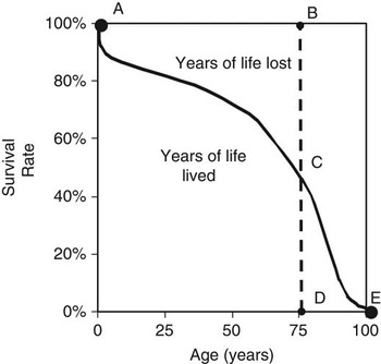
The perspectives of ‘attainment’ and ‘deprivation’ can also be seen in the field of demography, particularly in the context of the life table. The particular concept of interest is the survival curve. This depicts the temporal mortality experience of a cohort born in a particular year. The curve splits the space into two regions, viz. years of life lived, and years of life lost due to premature mortality. It is well known that survival curves shift through time, given various factors such as improved nutrition, medical/surgical interventions, etc. Such factors led Fries (Reference Fries1980) to speak of ‘the rectangularisation of the survival curve’ for high-income countries.
Figure 1 indicates a survival curve for a particular population (a cohort of 100,000 born in year 1) with an arbitrary cut-off at 100 years. The area below the survival curve measures the years of life lived by the hypothetical cohort, and the area above the curve indicates the PYLLs by the cohort. Let us assume that life expectancy at birth is 75 years, which is the dashed line BD in Figure 1.Footnote 8
Survival curve measuring the life years in a hypothetical cohort of 100,000 population born in year 1

The scholars who first studied the distribution of health per se (Silber, Reference Silber1982, Reference Silber1983, Reference Silber1988; Le Grand, Reference Le Grand1987, Reference Le Grand1989; and Illsley and Le Grand, Reference Illsley and Le Grand1987) were concerned with analysing the years of life lived before death, or more simply the distribution of age-at-death (the area below the survival curve in Figure 1). In other words, they were concerned with attainment, as outlined in, say, the Human Development Report (United Nations Development Programme, 1990). The PYLL, given it relates to the area above the survival curve, can be appropriately conceived of as a ‘deprivation’ measure. (As we note below, its distribution can be determined by calculating the Gini coefficient, as well as other measures of dispersion.)
Data sources
Perfect data sets rarely exist for social phenomena requiring analysis. In the case here, the concepts SLfS and Is/Es are being measured. Count data are readily available from the Australian Institute of Health and Welfare (AIHW) (2005) or from the Australian Bureau of Statistics (ABS) (2000). We note the (virtually) universal practice of using a count of the number of suicides (or one of its variants, such as the rate per 100,000 population) to measure what is referred to here as the SLfS but we wish in this section to consider an alternative measure of these concepts. The way we proceed here is to employ the PYLL measure of the SLfS as another demographic measure. The PYLL, first advocated by Dempsey (Reference Dempsey1947), places emphasis on the length of time lost, or length of life (measured in years) lost, due to premature death.Footnote 9
It is fairly commonplace that a particular variable cannot be directly observed or measured in empirical economics: an example is Friedman’s (Reference Friedman1957) notion of ‘permanent income’, an unobservable, whereas current income can be observed and measured, and it can be an indicator of permanent income. ‘Mismatch’ occurs to some extent between the concept and the measure of the concept, suggesting that some measurement error can arise. There is an econometric literature on measurement error, stemming from Goldberger (Reference Goldberger1971, Reference Goldberger1973) and Jöreskog and Goldberger (Reference Jöreskog and Goldberger1972), that is, the latent variable approach. This approach recognises that there is no exact measure of the theoretically appropriate concept (i.e. the SLfS and Is/Es). This literature argues that, instead, various proxy measures may be required. The headcount of suicides is an example of a proxy measure, but it is subject to some measurement error (Doessel et al., Reference Doessel, Williams and Whiteford2009a, Reference Doessel, Williams and Whiteford2009b).Footnote 10
Various measures, each imperfect, can shed some light on the welfare impact from mortality due to suicide. In this study, SLfS is measured by the PYLL, which enables the quantity of mortality to be quantified,Footnote 11 and measurement of the equality or inequality of the age distribution of suicide (i.e. the Is/Es) via the PYLL is also feasible.Footnote 12 To our knowledge, there is no prior study, which measures the age distribution of suicide.
The generated data for this study
The concept behind a PYLL calculation is relatively straightforward: choose an arbitrary potential limit to life; the life that is lost from premature death is the difference between that limit and age-at-death. Further elaboration of PYLL calculation is available elsewhere.Footnote 13
Having determined the life lost (measured in years), measures of inequality in a set of suicide PYLLs data can also be applied. In other words, from the PYLL data, we calculated measures of inequality. We applied two measures: the coefficient of variation (COV) and the Gini coefficient, for male and female PYLL rates, from 1907.
The use of two measures relates to the fact that, in inequality measurement exercises, it is almost always necessary to provide more than a single measure of inequality, as each measure can give a different result. There are underlying assumptions about inequality implied in each measure. This point is well established in the literature on income inequality measurement (e.g. Pen, Reference Pen1971; Cowell, Reference Cowell1995; Champernowne and Cowell, Reference Champernowne and Cowell1998; Creedy, Reference Creedy1998), that is, that the various measures of a distribution are summary measures, and that each involves different implicit assumptions about that distribution. All inequality measures produce different rankings and the only way one can have confidence in the conclusions of any inequality study is to check whether the rankings remain stable under different measures. Illustrations of this phenomenon for mental health services are available in Williams and Doessel (Reference Williams and Doessel2006). This study applies just two measures, but further work needs to be done to measure the inequality phenomenon more thoroughly.
Thus, this study involves several data sets. Two data sets were generated on the quantity or level of suicide and four time-series measures of inequality for Australia. These two sets are for the PYLL(75)AS(S) rate per 100,000 population, males and females from 1907 to 2003, and also the (headcount) mortality rate (MRAS(S)) for suicide, males and females for the same time period. Four time-series measures were then calculated for inequality measurement purposes: two inequality measures are applied to suicide, that is, COV and Gini, and both of these calculations were undertaken for males and females.
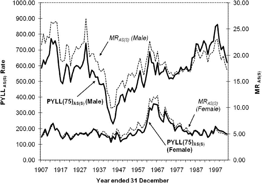
In Figure 2, we reproduce the two measures of the suicide rate applied here, for both males and females: the measure based on the PYLL, and the other based on the headcount rate MRAS(S). The data in Figure 2 indicate the trend in suicide (as measured here), for Australia, from 1907 to 2003. All rates are age standardised to the year 1991, and the potential length of life is assumed to be 75 years. Note the marked differences between the male and female rates.
Potential years of life lost (age standardised) per 100,000 population and the mortality rate (age standardised) per 100,000 population, suicide, males and females, Australia, 1907–2003
Source: Calculated from data in AIHW (2005).
Note: MRAS(S) is the mortality rate, age standardised, for suicide per 100,000 population, per year. The PYLL (75)AS(S) rate is the age-standardised total number of potential years of life lost [PYLL(75)] to suicide per 100,000 population, per year.
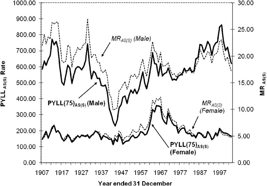
These are the data used to answer the first research question, viz. what is the statistical evidence for the rate of suicide for males, and for females, having increased, decreased or having remained constant through time in Australia? The data are analysed statistically, as described below, and the results are reported shortly.
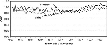
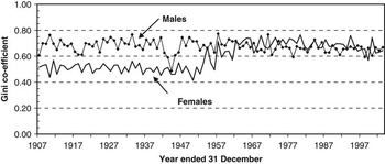
Our calculations of inequality measurements are employed to answer our second research question: has the age distribution of suicide for males, and for females, increased, decreased or remained constant through time in Australia? See Figures 3 and 4. These rates appear to be quite different between the genders and between the two measures of dispersion. This difference is to be expected, as the formulae for the COV and the Gini are quite dissimilar.


Statistical analysis
The research questions are answered by statistically modelling these time-series data sets, just described, using E-Views (Quantitative Micro Software, 2000). For the first research question, equation
(3)presents a general polynomial form, that is, to the kth power:

where St M/F is the quantity of suicide [the PYLL(75)AS(S) rate, and the MRAS(S)] for males/females at time period t, Xl is a vector of historical variables that may affect St M/F, μt is a ‘well-behaved’ error term, and α 0,α 1,…,αl are parameters to be estimated.
The approach employed for finding the equation-of-best-fit is Ordinary Least Squares modelling of the data. Apart from the application of conventional Goodness-of-Fit tests, a battery of diagnostic tests of the residuals and of the model specification was also applied. In this testing process, we checked for the extent of serial correlation and heteroscedasticity; all equations were also tested for normality of the residuals using the Jarque-Bera test, and the Augmented Dickey-Fuller test indicated whether or not the residuals were stationary. The Ramsey RESET specification test was applied to determine the appropriateness of the model specification.
Let us turn attention first to the trends through time in Australian suicide, male and female, as measured by the PYLL(75)AS(S) rate per 100,000 population, depicted in Figure 2. Casual observation of the data suggests some non-linearity, and general-to-specific methodology suggests that it is suitable to commence, say, with a fifth order polynomial.
Different eras in suicide behaviour through time are apparent in the data presented in Figure 2, suggesting that the incorporation of dummy variables may be relevant. In other words, these dummy variables are employed in modelling outlier observations that are present in the time-series.
For modelling the trends relating to the second research question (concerning the age distribution of age-at-suicide through time, as measured by the COV and the Gini coefficient), a general functional form is given in equation
(4):

where SI t M/F is suicide inequality (the COV or the Gini) for males/females at time period t; Xl is a vector of historical variables that may affect SI t M/F; γt is white noise (and another ‘well-behaved’ error term); and β 0, β 1,…, βl are parameters to be estimated. Again, with different eras in suicide behaviour through time, it may also be relevant to incorporate dummy variables in the inequality equations in order to model outlier observations that exist in the time-series.
The purpose of the diagnostic testing is to provide some confidence that the coefficients of the ‘best fit’ equation for each measure are not spurious. A second purpose is to provide the magnitude of, and extent to which, suicide (as measured) and its age distribution has risen, fallen or remained constant through time. It is instructive to note also that the modelling task involved more than a curve-fitting exercise: variation in suicide behaviour through time is apparent and the statistical analysis has additionally enabled the detection of different periods of suicide.
Statistical results
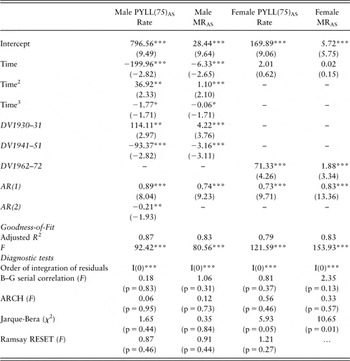
The results for the equations fitted to the PYLL(75)AS(S) rate (males and females) and the MRAS(S) (male and female) are presented in Table 1. Generally these equations perform well in terms of Goodness-of-Fit and the diagnostic tests. See also the details about the diagnostic testing which are found in Notes iii. to ix. of Table 1. Thus, there is reason to have some confidence in these statistical results.
Estimated time trends, PYLL(75)AS rate and headcount mortality rate, MRAS per 100,000 population, suicide, males and females, Australia, 1907–2003

PYLL = potential years of life lost; MR = mortality rate; DV = dummy variable; AR = autoregressive error; ARCH = autoregressive conditional heteroscedasticity.
Notes: (i) One, two and three asterisks indicate statistical significance at the 10%, 5% and 1% levels, respectively; (ii) DV1930–31 is a dummy variable that takes the value of unity from 1930–1931, and so forth for DV1941–51 and DV1962–72; (iii) AR(1) is the first-order coefficient of autocorrelation, and so forth; (iv) Data in parentheses are t-statistics. For the diagnostic tests, the p-values are in parentheses; (v) I(0) indicates that the residuals are ‘integrated of order zero’. Asterisks attached indicate that the Augmented Dickey-Fuller test statistic is statistically significant at the one, 5% and 10% levels, respectively; (vi) B–G serial correlation is the Breusch-Godfrey test, an F-test of the hypothesis that the residuals of the regression are not serially correlated; (vii) ARCH is an F-test of the hypothesis that autoregressive conditional heteroscedasticity is absent from the residuals; (viii) Jarque-Bera is a χ 2-test of the hypothesis that the distribution of the residuals is normal and (ix) Ramsay RESET test is an F-test of the hypothesis that the specification of the equation is correct.
Source: Calculated from data in AIHW (2005).
Note the several (period) dummy variables in this Table. For example, DV1930-31 is a dummy variable that takes the value of unity from 1930 to 1931, and so forth. The ‘best fit’ equation on the male PYLL data involves a rising quadratic with two dummy variables and two autoregressive error (AR) terms to address serial correlation. The recent decline in suicide proved insufficient in magnitude for a cubic form to pass the Ramsey RESET test, although we have reported the cubic term in Table 1. The estimated equation for male MRAS(S) for suicide in Table 1 indicates that both the equations (for the count and PYLL measures) are generally the same structurally, in terms of the signs of the coefficients and their significance. The large differences in values are due to the different measures.
The ‘best fit’ equation for female PYLLs incorporates a single dummy variable, DV1962–2003 but, otherwise, it is linear, with an AR term. The statistically significant coefficient on the dummy variable suggests 1962 began another era of female suicide. As with the results for males, the female equations are, in general, the same structurally, in terms of the signs of the coefficients and their significance for the two measures, although the values are very different. This is not surprising, as we have been considering two measures of the same phenomenon.
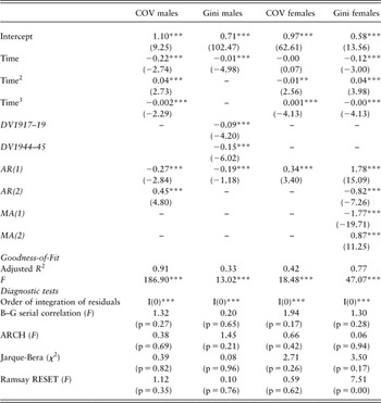
The equations estimated on the dispersion measures are presented in Table 2. The results are for equations fitted to the COVs (males and females), and the Gini coefficients, on the distribution of PYLL-based measures of age-at-suicide. ‘Saucer-shaped’ cubic equations using non-linear least squares performed well for both males and females in terms of Goodness-of-Fit, and also passed the diagnostic tests, upon the inclusion of AR terms. The results for the equations, male and female, on the Gini coefficients involve different equations in structural terms. The ‘best fit’ equation of the male Ginis is downward sloping and linear with two dummy variables, associated with World War I and World War II. The intercept of 0.71 is a relatively high value for the Gini coefficient, that is, indicating relative inequality. The equation for the female Gini data differs, once again, from that for the males, and note the intercept of 0.58 is lower than that for males.
Estimated time trends of coefficients of variation and Gini coefficients on age-standardised PYLLs from suicide, males and females, Australia, 1907–2003

The statistical work undertaken here is that of an initial study. Further research is clearly necessary. Statistical analysis has been undertaken to determine if the PYLL data exhibit periods of structural change that coincide with historical events or periods, for example, war, economic depressions, etc. but further analysis is needed to answer interpretative, and other, questions. For example, one next step is to use this PYLL measure of suicide in a multi-factorial causal model to ‘explain’ the suicide thus measured.
Interpreting PYLL-based suicide measures
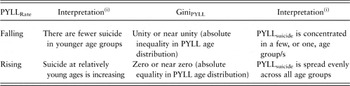
Broadly speaking, a declining PYLL rate indicates that relatively fewer suicides are occurring among younger age groups. A rising PYLL rate indicates relatively more youth suicide. However, the interpretation of Gini coefficients on PYLL distributions is a little more complicated. Recall that for an income distribution, a Gini coefficient of unity indicates perfect inequality in a distribution, while a Gini of zero indicates a perfectly equal distribution. With PYLL data, a very high Gini coefficient indicates the PYLLs are unevenly spread across all age groups, whereas a very low, or zero, Gini coefficient on suicide PYLLs data indicates the PYLLs are evenly spread across all age groups. Table 3 summarises these broad interpretations.
Interpretation of PYLL-based suicide measures

PYLL = potential years of life lost.
Note: (i) See Discussion section and also Table 4 for welfare implications.
One must approach the interpretation of trends in PYLL rates and distributions with caution. It is more difficult to interpret movements in the PYLL rate and Gini coefficients when they take intermediate values between the extreme values. This point is taken up again with Table 4 in the Discussion section below.
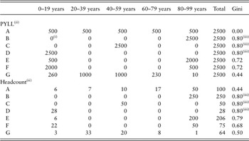
Some illustrative data showing seven PYLL(100) distributions, and related suicide mortality distributions, by age, and the Gini coefficient for each distribution

PYLL = potential years of life lost.
Note:
(i) For Gini coefficient calculations, zeros must be converted to an approximation of zero, for example, 0.00000001; (ii) It is assumed that the cohort has a constant population of 100,000 and (iii) That the Gini coefficient is not unity, given that the data appear to be completely unequal, is an artefact of there being a small number of observations.
Reductions in PYLLs in some age groups will, for example, usually unequally offset increases in PYLLs in other age groups. It is important to examine PYLL-based measures simultaneously with mortality rates. Both measures are relevant. It is also important to realise that value judgements are implicit in all such measures, a matter to which attention now turns in the Discussion section.
Discussion
Extensions of modern welfare economics provide a justification for time to enter the social welfare function, though this conception may not be accepted by all people: some may admire the suicide of honour, epitomised by the acts of inter alia Seneca, Lucretia, Brutus and Portia and Mark Anthony. For others, suicide is an act of personal autonomy, free will or self-determination, and people in the West are often puzzled by sati (or suttee), the Indian funeral custom in which a widow immolates herself alive on her husband’s funeral pyre. In addition, in existentialist thought, the concept of ‘the absurd’ leads to suicide being regarded as quite understandable: as there is no purpose, value or meaning in the world or to life, suicide is an obvious response.Footnote 14 Indeed, for Camus (Reference Camus1955), suicide was the ‘one truly serious philosophical problem’, and his answer was to struggle and revolt against the absurd (Camus, Reference Camus1948). Rebellion, for Camus, implies dissatisfaction with the human condition, that is, one needs to face the absurd, and make a decision in favour of life. See Lengers (Reference Lengers1994) for a discussion of Camus’ perspective for the role of health professionals. Given that philosophical qualification, the suicide prevention policies and strategies of a number of Western countries can be understood as a non-controversial dimension of the traditional discourse of modern welfare economics. This point is elaborated in Doessel et al. (Reference Doessel, Williams, Robertson and Whiteford2006).
With respect to measurement, some emphasis has been placed here on an alternative measure of the magnitude of suicide, the PYLL measure. The health literature on suicide in Australia uses only data based on a simple headcount of suicides, and various quotients based on this count measure. The alternative PYLL measure also has useful quantitative characteristics, and it has been employed in the empirical work here.
We re-emphasise the reason for applying more than a single measure of inequality to a distribution. It is well-established in the economic literature on measuring income inequality that each measure of inequality is based on implicit assumptions about the social welfare function (Pen, Reference Pen1971; Cowell, Reference Cowell1995; Champernowne and Cowell, Reference Champernowne and Cowell1998; Creedy, Reference Creedy1998). Inequality is measured generally in economics not just by statistical instruments, such as the COV, but also by other economic measures of inequality, such as the Gini coefficient, Lorenz curves and so forth. (See Williams and Doessel, Reference Williams and Doessel2006.) This study uses Gini coefficients, as well as COVs, in order to show that no single measure of inequality is sufficient. Such measures ought to be regarded as relevant to the age distribution of PYLLs and also to the age distribution of deaths per se.
Some emphasis here is placed on measuring the distribution of suicide. Suicide tended, in earlier periods, to be an occurrence among older persons, males especially, but since the 1950s, circumstances have changed and suicide is now more prevalent among relatively younger people. Although male suicide PYLLs are currently three to four times higher than female PYLLs, the female PYLLs are now double the level of 100 years ago. Thus, it is important to describe accurately the trends in suicide by age.
From the societal perspective, if death by suicide is to occur in any population, it could be argued that it is (generally speaking) better that death (from any cause) occurs as late in the life span as possible, with as little variation or dispersion in that late age as possible. Thus, from the societal perspective, it is ‘best’ if the distribution by age of suicide is unequal, with the age inequality concentrated at later age groups.Footnote 15
It seems that the current policy goal of averting the high level of youth suicide is unequivocal. Indeed we do not wish to undermine any such view. However, one must still be careful to ask what is foregone in pursuing a declining PYLL rate in a population, an implicitly attractive goal. Even if suicide policy were successful in achieving a declining PYLL rate, policy makers still need to be informed about the characteristics that have changed in the age distribution of PYLLs and the age distribution of deaths. There are important welfare implications behind trends in suicide and one must therefore approach the interpretation of trends in PYLL rates and distributions with caution.
This point is illustrated by Table 4, which provides seven cases (A–G) of illustrative data on PYLLs across five age groups. The data are generated such that the age distribution of PYLLs across the cases varies but the total of PYLLs remains constant. The Table shows also how the age distribution of (headcount) deaths due to suicide is associated with each of the seven PYLL distributions. Gini coefficients are calculated on the age distributions of both PYLLs and headcount mortality, and show some of the disparities that exist across the cases.
We do not wish to enter debate here over which of the seven PYLL distributions in Table 4 is ideal. We also do not want to attempt to rank these seven cases in order from best to worst. However, we do wish to argue for policy makers to be informed of all aspects of suicide policy. The approach to suicide measurement here is also particularly useful for making comparisons, such as those employed here through time or by gender, or by locality, ethnic or income group and so forth. Being informed about the effectiveness of suicide policy requires suitable and sufficient measures of suicide.
In conclusion, this study provides a ‘story’ about Australia’s experience of suicide reduction that captures other information from that currently available: it goes beyond the suicide measures that are being conventionally applied. Three key points can be concluded, as follows.
In answer to our first research question on the Social Loss from Suicide, we find that the ‘best fit’ equation for males on both PYLL data and conventional headcount data is a rising quadratic with two (period) dummy variables. The decline in suicide in more recent years, which is insufficient for a cubic form, suggests the view that there has been a recent downturn in suicide is too sanguine, when one takes a longer term view of the century of data. For females, the ‘best fit’ equation is linear for both measures, with a single (period) dummy variable, DV1962–72. More work needs to be done to understand these periods of male and female suicide.
In answer to our second research question on the distribution of the Social Loss from Suicide, ‘saucer-shaped’ cubic equations for COVs for both males and females have been determined. The equations, both for males and females, on the Gini coefficients are different in structural terms from the COVs, and reasons for this are given. The ‘best fit’ equation of the male Ginis is downward sloping and linear with two dummy variables, associated with World War I and World War II. The relatively high intercept value for the Gini coefficient for males indicates relative inequality. For females, the Gini equation differed in structure from that for the males, and the intercept indicates lesser inequality for females than for males, on PYLL data.
The third point relates to interpreting the results. Our illustrative Tables 3 and 4 above demonstrate the importance for policy makers of informing themselves of all aspects of suicide measurement and policy. Being informed about the effectiveness of suicide policy requires measures of the welfare impact of suicide, that are suitable and sufficient in terms of the social loss per se from suicide and the distribution of that loss.
Finally, it is appropriate to qualify the conclusions here in terms of the adage: ‘more work needs to be done’.
Acknowledgements
This is a revised version of a paper presented to the College des Economistes de la Sante – Health Economists’ Study Group Workshop, 4–6 January 2006, City University, London, and at the School of Population Health, The University of Queensland, Brisbane, 21 March 2006. The authors are very grateful for the helpful comments of two anonymous referees. Financial assistance of the Queensland Government is acknowledged. Any remaining errors and omissions are our own responsibility.