



1. Introduction
Linear optimal initial conditions for the flow in an axial corner are considered. The classical corner-flow problem, as sketched in figure 1, consists of two right-angled, semi-infinite flat plates with the potential flow
 $u_{\infty }$
aligned with the intersection line. Here,
 $x$
denotes the streamwise direction, and the two spanwise coordinates
 $y$
and
 $z$
span the transversal plane. In addition, a
 $45^{\circ }$
-rotated, auxiliary coordinate system is introduced with its abscissa
 $s$
along the corner bisector. A set of equations based on the Blasius similarity transformation and matched asymptotic expansions, the so-called corner-flow equations, was derived by Rubin (Reference Rubin1966). They describe the laminar, incompressible flow in the transversal corner plane and were first solved numerically by Rubin & Grossman (Reference Rubin and Grossman1971). As far-field boundary conditions, the authors relied on the solution of an additional set of equations governing the asymptotic secondary cross-flow induced by the superposition of the displacement effects of the two plates (Pal & Rubin Reference Pal and Rubin1971). Detailed overviews of many numerical corner-flow studies can be found in the works of Ridha (Reference Ridha2003), Galionis & Hall (Reference Galionis and Hall2005) and Schmidt & Rist (Reference Schmidt and Rist2011). The topics include the effects of compressibility (Weinberg & Rubin Reference Weinberg and Rubin1972), a non-zero streamwise pressure gradient (Ridha Reference Ridha1992) and arbitrary corner angles (Barclay & Ridha Reference Barclay and Ridha1980). The main difficulty in corner-flow computations stems from the observation that the influence of the corner on the cross-flow field does not decay exponentially with increasing distance from the intersection line. Consequently, either a sufficiently large computational domain has to be chosen or a coordinate transform that maps the far-field boundaries to true infinity as realized by Ghia (Reference Ghia1975) and Mikhail & Ghia (Reference Mikhail and Ghia1978) has to be applied.
Sketch of the flow in a streamwise corner (Schmidt & Rist Reference Schmidt and Rist2011).

Numerous linear stability analyses based on the self-similar corner-flow solutions mentioned above have been conducted in the past, starting with studies of one-dimensional velocity profiles of the blending boundary layer between the corner region and the asymptotic far-field solution by Lakin & Hussaini (Reference Lakin and Hussaini1984), Dhanak (Reference Dhanak1992, Reference Dhanak1993) and Dhanak & Duck (Reference Dhanak and Duck1997). The two-dimensional linear stability problem for the self-similarity solution was first addressed by Balachandar & Malik (Reference Balachandar and Malik1995) within an inviscid framework. The effect of a streamwise pressure gradient was included in the viscous corner-flow stability study by Parker & Balachandar (Reference Parker and Balachandar1999), the influence of compressibility in Schmidt & Rist (Reference Schmidt and Rist2011) and the spatial non-parallel stability problem was examined by Galionis & Hall (Reference Galionis and Hall2005) and Alizard, Rist & Robinet (Reference Alizard, Rist and Robinet2009) by solving the parabolized stability equations.
Despite the different approaches taken, a major inconsistency between numerical studies and experimental surveys remains unsolved. While linear stability analyses of the self-similar base state predict a critical Reynolds number of
 $\mathit{Re}_{x,c}\approx 9\times 10^{4}$
(Balachandar & Malik Reference Balachandar and Malik1995; Parker & Balachandar Reference Parker and Balachandar1999; Galionis & Hall Reference Galionis and Hall2005; Schmidt & Rist Reference Schmidt and Rist2011), experimental evidence suggests a transitional Reynolds number as low as
 $\mathit{Re}_{x,c}\approx 10^{4}$
(even for a small favourable pressure gradient). Experimental data from more than two decades starting with early measurements by Nomura (Reference Nomura1962) was collected and compared with each other and with theory by Zamir (Reference Zamir1981). The reader is referred to this comprehensive aggregation of data for an insight into the experimental evidence. A major point of discussion is the validity of the self-similarity solution as measurements commonly show a deviation from the theoretical laminar flow in the near-corner region. Kornilov & Kharitonov (Reference Kornilov and Kharitonov1982) attributed the deviation to the pressure field induced by the intersection of the plates in the leading-edge region in their experimental study.
Balachandar & Malik (Reference Balachandar and Malik1995) explained the discrepancy between experiment and theory by the presence of an inviscid mechanism in the corner region. They found a critical Reynolds number of
 $\mathit{Re}_{x,c}=435$
for the one-dimensional bisector-profile instability but could not confirm this number for the two-dimensional problem. A nonlinear mechanism was brought into the discussion as a possible cause by Galionis & Hall (Reference Galionis and Hall2005). Only recently, Alizard, Robinet & Rist (Reference Alizard, Robinet and Rist2010) computed the sensitivity of the self-similar corner-flow solution with respect to base-flow variations and suggested a transient growth mechanism to explain the low transitional Reynolds number. In this paper, we follow that route and assess the question of how much kinetic energy a localized perturbation can maximally gain from the mean flow while being advected downstream over some finite time
 ${\it\tau}$
. This is done by computing global optimal initial conditions that are artificially restricted to a finite streamwise extent. A time-stepper-based optimization technique, as introduced by Monokrousos et al. (Reference Monokrousos, Åkervik, Brandt and Henningson2010) for the computation of optimal solutions for flat plate boundary layer, is employed for that purpose. The artificial localization of the optimal initial condition is a numerical necessity caused by the spatial inhomogeneity of the base flow. The resulting response manifests in form of a wavepacket. The use of optimization techniques to calculate optimal perturbations in fluid dynamic applications dates back to Farrell (Reference Farrell1988), who calculated the optimal excitation in constant shear flow, first in two and later in three dimensions (Butler & Farrell Reference Butler and Farrell1992; Farrell & Ioannou Reference Farrell and Ioannou1993). The authors found three-dimensional optimal structures which exhibit large energy growth despite the absence of unstable normal modes. Two already known mechanisms were identified as the main causes of non-modal growth. First, the Orr mechanism (Orr Reference Orr1907; Lindzen Reference Lindzen1988) that allows perturbation waves whose fields of constant phase are initially inclined against the mean shear to extract energy from the base flow by adopting to the mean shear while being convected downstream. Second, the lift-up mechanism as described by Ellingsen & Palm (Reference Ellingsen and Palm1975) and Landahl (Reference Landahl1975, Reference Landahl1980). It describes the generation of streamwise streaks caused by momentum transfer from vortical structures in the cross-flow plane to the streamwise velocity component. The lift-up of a low-speed streak leads to an inflection point in the streamwise velocity profile and, hence, gives rise to an inviscid instability of secondary nature. The Orr and the lift-up mechanisms were identified by Monokrousos et al. (Reference Monokrousos, Åkervik, Brandt and Henningson2010) on the flat plate as the origin of transient growth for long and short optimization times, respectively. In recent work by Alizard, Robinet & Guiho (Reference Alizard, Robinet and Guiho2012), the authors investigated the non-modal behaviour of the self-similar corner-flow solution within a parallel framework, and found that the same two effects lead to substantial transient growth. The maximum gain was achieved by optimal structures that are antisymmetric with respect to the corner bisector. In a direct numerical simulation (DNS) conducted by Schmidt & Rist (Reference Schmidt and Rist2014), it was found that corner flow is prone to spatial transient growth under harmonic forcing at subcritical Reynolds numbers. It was demonstrated that pseudo-resonance between the inviscid corner mode and viscous branch solutions causes a moderate transient perturbation amplification. The present study elaborates on the non-modal worst-case scenario in form of linear global optimal perturbations. The results are put in the context of the last mentioned DNS findings, the computations by Alizard et al. (Reference Alizard, Robinet and Rist2010, Reference Alizard, Robinet and Guiho2012) and the investigation of the related flat-plate flow by Monokrousos et al. (Reference Monokrousos, Åkervik, Brandt and Henningson2010). In fact, the present work can be regarded as a continuation of the aforementioned studies: the transient growth study by Alizard et al. (Reference Alizard, Robinet and Guiho2012) is extended by incorporating non-parallel effects, and the survey on optimal disturbances by Monokrousos et al. (Reference Monokrousos, Åkervik, Brandt and Henningson2010) by considering a fully three-dimensional base state, i.e. without homogeneity in the spanwise direction.
The paper is organized as follows: the governing equations and theoretical concepts are introduced in § 2. Subsequently, their numerical implementation is explained in § 3. The main part of the paper consists of the presentation and interpretation of the results of the global non-modal study in § 4. Prior to this, the two base states are presented and a classical local stability and sensitivity analysis is conducted. The paper ends with a summary of the results and a comparison with previous literature in § 5.
2. Theoretical background
The governing equations and their linearized counterpart are presented in § 2.1. Under the assumption of infinitesimally small wave-like perturbations, the eigenvalue problem (EVP) of classical linear stability theory is obtained in § 2.2. The
 ${\it\epsilon}$
-pseudospectrum-based sensitivity analysis of linear operators is recapitulated in the same section. Finally, the theory of global linear optimals which is at the basis of the present study is addressed in § 2.3.
2.1. Governing equations
The motion of an incompressible fluid in a domain
 $\mathscr{D}$
is governed by the incompressible Navier–Stokes equations supplemented by the continuity equation
 $$\begin{eqnarray}\frac{\partial \boldsymbol{u}}{\partial t}=-\left(\boldsymbol{u}\boldsymbol{\cdot }\boldsymbol{{\rm\nabla}}\right)\boldsymbol{u}-\boldsymbol{{\rm\nabla}}p+\frac{1}{\mathit{Re}}{\rm\nabla}^{2}\boldsymbol{u},\quad \boldsymbol{{\rm\nabla}}\boldsymbol{\cdot }\boldsymbol{u}=0\,~\text{in}\;\mathscr{D},\end{eqnarray}$$
where
 $\boldsymbol{u}(\boldsymbol{x},t)=[u\;v\;w]^{\text{T}}\,(x,y,z,t)$
is the vector of Cartesian velocity components and
 $p(x,y,z,t)$
the pressure. Here
 $\mathit{Re}=u_{\infty }{\it\delta}/{\it\nu}$
is the Reynolds number based on some characteristic length
 ${\it\delta}$
, the far-field velocity
 $u_{\infty }$
and the kinematic viscosity
 ${\it\nu}$
. Velocities are non-dimensionalized by
 $u_{\infty }$
, Cartesian coordinates by
 ${\it\delta}$
, and a unit density is assumed. Here, we choose
 ${\it\delta}\equiv {\it\delta}^{\ast }(x_{0})$
, where
 ${\it\delta}^{\ast }=\int _{0}^{\infty }(1-U/u_{\infty })\text{d}y$
is the displacement thickness of the one-dimensional far-field velocity profile which coincides with the classical Blasius boundary layer solution for the streamwise and wall-normal velocity components. Here
 $x_{0}$
refers to the start of the computational domain. The Navier–Stokes equations (2.1) can be linearized by Reynolds decomposing the velocity and pressure fields into a steady base flow
 $\{\boldsymbol{U}(\boldsymbol{x}),\;P(\boldsymbol{x})\}$
, which is a solution to (2.1) itself, and a small perturbation
 ${\it\epsilon}\{\boldsymbol{u}^{\prime }(\boldsymbol{x},t),\;p^{\prime }(\boldsymbol{x},t)\}$
, i.e.
 $\boldsymbol{u}=\boldsymbol{U}+{\it\epsilon}\boldsymbol{u}^{\prime }$
, and
 $p=P+{\it\epsilon}p^{\prime }$
. The linearized Navier–Stokes equations
 $$\begin{eqnarray}\frac{\partial \boldsymbol{u}^{\prime }}{\partial t}=-(\boldsymbol{U}\boldsymbol{\cdot }\boldsymbol{{\rm\nabla}})\boldsymbol{u}^{\prime }-\left(\boldsymbol{u}^{\prime }\boldsymbol{\cdot }\boldsymbol{{\rm\nabla}}\right)\boldsymbol{U}-\boldsymbol{{\rm\nabla}}p^{\prime }+\frac{1}{\mathit{Re}}{\rm\nabla}^{2}\boldsymbol{u}^{\prime },\quad \boldsymbol{{\rm\nabla}}\boldsymbol{\cdot }\boldsymbol{u}^{\prime }=0\,~\text{in}\;\mathscr{D}\end{eqnarray}$$
are obtained by keeping only terms that are linear in the bookkeeping variable
 ${\it\epsilon}$
or, equivalently, by neglecting products of small quantities. Problem-dependant boundary conditions are enforced on the boundaries
 $\partial \mathscr{D}$
.
2.2. Local linear stability theory
In classical local linear stability theory, wave-like (normal-mode) solutions of the form
 $\boldsymbol{q}^{\prime }(y,z,t)=\hat{\boldsymbol{q}}(y,z)\;\text{e}^{\text{i}({\it\alpha}x-{\it\omega}t)}$
upon a parallel laminar base-state
 $\boldsymbol{Q}(y,z)$
are considered, where
 $\boldsymbol{q}^{\prime }$
and
 $\boldsymbol{Q}$
represent the solution vector of perturbation flow quantities and the corresponding base-state, respectively. Inserting the normal-mode ansatz in (2.2) gives an EVP for the amplitude function
 $\hat{\boldsymbol{q}}$
with the complex streamwise wavenumber
 ${\it\alpha}\in \mathbb{C}$
as the corresponding eigenvalue. Here, we let
 ${\it\omega}\in \mathbb{R}$
as we are interested in the spatial evolution of a harmonic wave at a given forcing frequency
 ${\it\omega}$
, i.e. in spatial stability. Spatial amplification is found for
 $\text{Im}\{{\it\alpha}\}<0$
. The resulting spatial linear stability EVP can be written in matrix (discretized) form as
 $(\unicode[STIX]{x1D647}_{0}+{\it\alpha}\unicode[STIX]{x1D647}_{1}+{\it\alpha}^{2}\unicode[STIX]{x1D647}_{2})\hat{\boldsymbol{q}}=0$
, and is of second order in the eigenvalue
 ${\it\alpha}$
. Most commonly, the second-order EVP is reduced to an extended linear EVP
 $$\begin{eqnarray}\left(\widetilde{\unicode[STIX]{x1D647}}_{0}+{\it\alpha}\widetilde{\unicode[STIX]{x1D647}}_{1}\right)\tilde{\boldsymbol{q}}=0\end{eqnarray}$$
through the introduction of a set of auxiliary variables
 $\tilde{\boldsymbol{q}}=[\hat{\boldsymbol{q}}\;{\it\alpha}\hat{\boldsymbol{q}}]^{\text{T}}$
. The reader is referred to the reviews by Mack (Reference Mack1984) and Theofilis (Reference Theofilis2003) for details on the subject.
The classical eigenvalue-based analysis outlined above describes the long-time response by considering the dominant eigenvalue of the linear system. For non-normal operators, however, significant (short-time) transient growth can occur as a result of the non-orthogonality of the solution space spanned by the eigenvectors (Reddy, Schmid & Henningson Reference Reddy, Schmid and Henningson1993; Trefethen et al.
Reference Trefethen, Trefethen, Reddy and Driscoll1993). The sensitivity of the spectrum to generally random perturbations to the governing linear operator can be quantified in terms of
 ${\it\epsilon}$
-pseudospectra as shown by Trefethen (Reference Trefethen1991). The reader is referred to the latter three references for details. By definition, a complex number
 ${\it\alpha}\in \mathbb{C}$
is said to be in the
 ${\it\epsilon}$
-pseudospectrum if
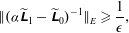 $$\begin{eqnarray}\Vert ({\it\alpha}\widetilde{\unicode[STIX]{x1D647}}_{1}-\widetilde{\unicode[STIX]{x1D647}}_{0})^{-1}\Vert _{E}\geqslant \frac{1}{{\it\epsilon}},\end{eqnarray}$$
where
 $({\it\alpha}\widetilde{\unicode[STIX]{x1D647}}_{1}-\widetilde{\unicode[STIX]{x1D647}}_{0})^{-1}$
is the resolvent and
 $\Vert \cdot \Vert _{E}$
some appropriate energy norm. For incompressible flows, the perturbation kinetic energy in form of the standard Euclidean 2-norm
 $\Vert \hat{\boldsymbol{u}}\Vert _{2}$
is chosen. The contours of the resolvent for some value
 ${\it\epsilon}$
can be interpreted as the upper bound for the eigenvalues of a randomly perturbed operator
 $\widetilde{\unicode[STIX]{x1D647}}_{0}+\unicode[STIX]{x1D640}$
, where
 $\unicode[STIX]{x1D640}$
is a random matrix of norm
 $\Vert \unicode[STIX]{x1D640}\Vert _{E}\leqslant {\it\epsilon}$
.
2.3. Global optimal disturbances
Within the framework of optimal initial conditions we are interested in finding a solution to (2.2), possibly subject to other constraints, that maximizes some measure of energy while evolving over a finite time span
 $t\in [0,{\it\tau}]$
. To do so, we first introduce the concept of a linear evolution operator
 $\mathscr{A}(t)$
that maps an initial perturbation
 $\boldsymbol{u}^{\prime }(t_{0})$
to
 $\boldsymbol{u}^{\prime }(t+t_{0})$
at some other time instant, i.e.
 $\boldsymbol{u}^{\prime }(t+t_{0})=\mathscr{A}(t)\boldsymbol{u}^{\prime }(t_{0})$
. Further, we use the standard
 $L_{2}$
inner product
 $\langle \boldsymbol{u},\boldsymbol{v}\rangle =\int _{\mathscr{D}}\boldsymbol{u}\boldsymbol{\cdot }\boldsymbol{v}\text{d}\mathscr{D}$
, which conveniently defines the norm associated with the kinetic energy of the perturbation
 $\Vert \boldsymbol{u}^{\prime }\Vert _{2}=\langle \boldsymbol{u}^{\prime },\boldsymbol{u}^{\prime }\rangle$
. As we are interested in the transient development of an initial perturbation, we first have to define a suitable measure of such, i.e. transient growth. The term refers to the ratio of the perturbation kinetic energy normalized by its initial condition at
 $t=0$
(Reddy & Henningson Reference Reddy and Henningson1993; Trefethen et al.
Reference Trefethen, Trefethen, Reddy and Driscoll1993), and can be recast in terms of the linear evolution operator as follows:
 $$\begin{eqnarray}G(t)\equiv \frac{E(t)}{E(0)}=\frac{\Vert \boldsymbol{u}^{\prime }(t)\Vert _{2}}{\Vert \boldsymbol{u}^{\prime }(0)\Vert _{2}}=\frac{\left\langle \mathscr{A}(t)\boldsymbol{u}^{\prime }(0),\mathscr{A}(t)\boldsymbol{u}^{\prime }(0)\right\rangle }{\left\langle \boldsymbol{u}^{\prime }(0),\boldsymbol{u}^{\prime }(0)\right\rangle }=\frac{\left\langle \boldsymbol{u}^{\prime }(0),\mathscr{A}^{\dagger }(t)\mathscr{A}(t)\boldsymbol{u}^{\prime }(0)\right\rangle }{\left\langle \boldsymbol{u}^{\prime }(0),\boldsymbol{u}^{\prime }(0)\right\rangle }.\end{eqnarray}$$
Here, the action of the adjoint operator
 $\mathscr{A}^{\dagger }$
is given by
 $$\begin{eqnarray}\left\langle \mathscr{A}\boldsymbol{u}^{\prime },\boldsymbol{u}^{\dagger }\right\rangle =\left\langle \boldsymbol{u}^{\prime },\mathscr{A}^{\dagger }\boldsymbol{u}^{\dagger }\right\rangle .\end{eqnarray}$$
By looking for the solution that maximizes the transient growth over some finite time
 ${\it\tau}$
we define the maximum growth
 $G_{max}({\it\tau})$
as
 $$\begin{eqnarray}G_{max}({\it\tau})\equiv \max _{\Vert \boldsymbol{u}^{\prime }(0)\Vert \neq 0}\frac{E({\it\tau})}{E(0)}=\max _{\Vert \boldsymbol{u}^{\prime }(0)\Vert \neq 0}\frac{\left\langle \boldsymbol{u}^{\prime }(0),\mathscr{A}^{\dagger }({\it\tau})\mathscr{A}({\it\tau})\boldsymbol{u}^{\prime }(0)\right\rangle }{\left\langle \boldsymbol{u}^{\prime }(0),\boldsymbol{u}^{\prime }(0)\right\rangle }.\end{eqnarray}$$
From (2.7), note that the last term in the equality corresponds to the induced matrix norm of
 $\mathscr{A}^{\dagger }({\it\tau})\mathscr{A}({\it\tau})$
. Hence, the dominant eigenvalue of
 $\mathscr{A}^{\dagger }({\it\tau})\mathscr{A}({\it\tau})$
(or singular value of
 $\mathscr{A}({\it\tau})$
, respectively) is the solution to the optimization problem (2.7).
The linear evolution operator
 $\mathscr{A}({\it\tau})$
and its adjoint counterpart cannot be formulated directly without the assumption of local eigenfunctions (Luchini Reference Luchini2000). However, the action of the evolution operator on an initial perturbation can be obtained from integrating the underlying initial value problem. From that perspective, the linear operator defined by (2.2) acts as the infinitesimal generator of the evolution operator
 $\mathscr{A}({\it\tau})$
(Edwards et al.
Reference Edwards, Tuckerman, Friesner and Sorensen1994). The action of the adjoint evolution operator
 $\mathscr{A}^{\dagger }({\it\tau})$
can be approximated in the same manner by integration of the adjoint equations corresponding to the linearized Navier–Stokes equations (2.2)
 $$\begin{eqnarray}-\frac{\partial \boldsymbol{u}^{\dagger }}{\partial t}=-(\boldsymbol{U}\boldsymbol{\cdot }\boldsymbol{{\rm\nabla}})\boldsymbol{u}^{\dagger }+\left(\boldsymbol{{\rm\nabla}}\boldsymbol{U}\right)^{\text{T}}\boldsymbol{\cdot }\boldsymbol{u}^{\dagger }-\boldsymbol{{\rm\nabla}}p^{\dagger }+\frac{1}{\mathit{Re}}{\rm\nabla}^{2}\boldsymbol{u}^{\dagger },\quad \boldsymbol{{\rm\nabla}}\boldsymbol{\cdot }\boldsymbol{u}^{\dagger }=0\,~\text{in}\;\mathscr{D}.\end{eqnarray}$$
Equations (2.8) are derived by substituting the linear operator defined by (2.2) into the left-hand side of (2.6), then integrating by parts the individual terms and subsequently recasting the equation in form of the inner product on the right-hand side of (2.6). Now note that applying
 $\mathscr{A}^{\dagger }({\it\tau})$
to
 $\mathscr{A}({\it\tau})\boldsymbol{u}^{\prime }(0)$
in (2.7) corresponds to taking
 $\boldsymbol{u}^{\prime }({\it\tau})$
as the initial condition for integrating the adjoint linearized Navier–Stokes equations (2.8). Together with the observation that (2.8) features a negative sign in front of the time derivative term, we see that the action of
 $\mathscr{A}^{\dagger }({\it\tau})$
evolves the initial perturbation backwards in time. A detailed derivation of the adjoint evolution operator and the adjoint Navier–Stokes equations can be found in Bagheri, Brandt & Henningson (Reference Bagheri, Brandt and Henningson2009).
3. Numerical methods
In the following, the numerical methods used for the calculation of the laminar base-states, the spatial local stability and sensitivity analysis and the global optimization are described in §§ 3.1–3.3, respectively.
3.1. Self-similar base-state calculation
Two laminar base states are considered in this study: the canonical self-similar solution as first obtained by Rubin (Reference Rubin1966) and used throughout literature, and an altered base-flow that better imitates experimental results. The canonical state is henceforth referred to as non-modified or zero pressure gradient (ZPG), and the second referred to as the modified base flow. The latter mimics the bulge-shaped deformation in the near-corner region as observed in experimental studies. Here, measurement data taken from the study by Zamir & Young (Reference Zamir and Young1970) serves as a reference. The exact form of the deformation depends on the leading-edge geometry and is a function of the position along the plates. Therefore, it renders the base-state non-self-similar and cannot be modelled accurately without taking into account the fully three-dimensional nature of the leading-edge flow, which is beyond the scope of this study. However, given the experimental reference, a body force term (or, equivalently, streamwise pressure gradient term) can be constructed that deforms the self-similar base-state in the desired manner. Both laminar base states are obtained as solutions to the parabolized Navier–Stokes (PNS) equations. Under the assumption of a steady laminar flow with negligible upstream effects, the fundamental equations can be simplified significantly, and be solved by a downstream space-marching procedure (see e.g. Tannehill, Anderson & Pletcher Reference Tannehill, Anderson and Pletcher1997). We employ the same code as used and validated in Schmidt & Rist (Reference Schmidt and Rist2011). The procedure used to converge self-similar base states employed in the present work is also described therein, as well as the computation strategy for the one-dimensional far-field solution required for the far-field boundary condition. The latter is based on the solution of a designated equation for the asymptotic secondary cross-flow profile (Ghia & Davis Reference Ghia and Davis1974) as described in more detail in Schmidt & Rist (Reference Schmidt and Rist2014). The so-obtained profile corresponds to the lower branch (Blasius-like) of the dual solution in the work of Ridha (Reference Ridha1992), who showed that two solutions to the incompressible corner-flow equations exist, even for a zero streamwise pressure gradient. It is the only solution permitted by our framework, and almost exclusively used throughout literature. The code shares the same Chebyshev-collocation-based spatial differentiation scheme with the linear stability code, and utilizes a first-order accurate implicit Euler method to advance the solution in the streamwise direction. The code is used as is for the calculation of the canonical ZPG solution.
For the calculation of the modified base state which mimics the bulge-shaped deformation, however, a code modification is required. We aim at reproducing the general effect of the deformation on stability by taking a reverse-engineering approach. First, a two-dimensional streamwise velocity field featuring the bulge deformation is reconstructed by interpolation and extrapolation of published hot-wire measurement data. Second, the latter field data is transformed into self-similar (Levy–Lees) coordinates and the difference to the self-similar solution, here termed
 ${\rm\Delta}U$
, is sought. Third,
 ${\rm\Delta}U$
is used within a body forcing term (or, equivalently, a localized streamwise pressure gradient) to obtain a self-similar base state featuring the same deformation. Self-similarity of the result is achieved by assuming a force term that is compatible with the well-known Falkner–Skan similarity transformation, i.e. to a viscous boundary-layer-type flow with a potential far-field solution that satisfies
 $U(x)=u_{\infty }x^{m}$
. The sign of the exponent
 $m$
determines whether the flow is accelerated (
 $m>0$
) or retarded (
 $m<0$
). For the flat-plate solution, boundary-layer separation occurs for
 $m\leqslant -0.091$
. Note that unlike for Falkner–Skan flow,
 ${\rm\Delta}U$
has compact support in our procedure as the interpolated experimental solution approaches the self-similar base state at some distance away from the close-corner region. In addition, we assume that the asymptotic corner-flow solution enforced on the far-field boundaries is valid for the forced model as well, i.e. that the outer boundaries are sufficiently far away from the region of influence of the forcing. In operator notation, the PNS system can be written compactly as
 $$\begin{eqnarray}\unicode[STIX]{x1D64B}\boldsymbol{Q}^{(i+1)}=\boldsymbol{r}+c{\rm\Delta}\boldsymbol{Q}mx^{2m-1}.\end{eqnarray}$$
Here,
 $\unicode[STIX]{x1D64B}$
is the discretized PNS operator, and the self-similar forcing term is added to the right-hand side
 $\boldsymbol{r}$
of the equation. For self-similarity, the forcing term must be of the same form as the streamwise pressure gradient equivalent to the above-mentioned potential flow distribution. A factor
 $c$
is introduced for the adjustment of the amplitude. The solution vector and the body force distribution vector are given by
 $\boldsymbol{Q}=[{\it\rho}\;U\;V\;W\;T]^{\text{T}}$
and
 ${\rm\Delta}\boldsymbol{Q}=[0\;{\rm\Delta}U\;0\;0\;0]^{\text{T}}$
, respectively. The density
 ${\it\rho}$
and temperature
 $T$
are part of the solution as the solver is written for a general compressible fluid. Incompressible limit solutions are obtained by considering the low-Mach-number regime, i.e. by setting
 $\mathit{Ma}=0.1$
for the case at hand. The temperature and density solution are omitted henceforth. The validity of the procedure is confirmed a posteriori: fully converged self-similar solutions were obtained for a range of amplitude factors
 $c$
and exponents
 $m$
. A satisfactory fit to the reference solution as presented later in § 4.1 was obtained for
 $m=-0.05$
and
 $c=2$
. The results presented in § 4.1 are obtained on a
 $50\times 50$
collocation point grid to resolve a domain of size
 $y,z\in [0,0]\times [50,50]$
. The large domain extent guarantees the validity of the asymptotic far-field solution, even for the modified base-state calculation. As in Schmidt & Rist (Reference Schmidt and Rist2011), a fast convergence towards a self-similar state was observed.
3.2. Spatial local stability calculation
The spatial local stability EVP (2.3) is solved by a shift-and-invert Arnoldi algorithm on a transformed Chebyshev-collocation grid as in Schmidt & Rist (Reference Schmidt and Rist2011). A spatial resolution of
 $45\times 45$
collocation points is used to resolve a domain of size
 $y,z\in [0,0]\times [35,35]$
, where the walls are situated at
 $y=0$
and
 $z=0$
, respectively. The spanwise coordinates are normalized by the local displacement thickness of the far-field solution. An algebraic grid stretching is applied to cluster half of the points in the wall-near 20 % of the domain along both walls. The 15 leading (usually 14 viscous Tollmien–Schlichting-type modes and the inviscid corner mode) modes are converged to a tolerance of
 ${\it\sigma}=10^{-6}$
for each
 $(\mathit{Re}_{x},{\it\omega})$
combination. For the construction of the stability diagrams in § 4.1, the frequency domain is resolved by 15 equally spaced points. Along the abscissa a resolution of 45 and 60 points is chosen for the ZPG and the modified base state, respectively. Table 1 summarizes the parameters used for the linear stability calculations presented in § 4.2. The efficient routines of the EigTool library (Wright Reference Wright2002) are employed to calculate the resolvent in (2.4) in the context of eigenvalue sensitivity.
Parameters of the spatial local stability calculation. Here
 $n_{Re}$
and
 $n_{{\it\omega}}$
are the number of data points along the Reynolds number and frequency axis, respectively. Here
 $N_{y}$
and
 $N_{z}$
are the number of Gauss–Lobatto points in the spanwise directions.

3.3. Global optimal disturbances with Nek5000
The actions of the linear evolution operator
 $\mathscr{A}$
and its adjoint
 $\mathscr{A}^{\dagger }$
are calculated by time integration of the linear direct and linear adjoint Navier–Stokes equations, (2.1) and (2.8), respectively. Both sets of equations are solved with the spectral element code Nek5000 (Fischer, Lottes & Kerkemeier Reference Fischer, Lottes and Kerkemeier2008) that was also used in the reference study by Monokrousos et al. (Reference Monokrousos, Åkervik, Brandt and Henningson2010). It uses semi-implicit time-stepping combined with a weighted residual spectral element method (Patera Reference Patera1984) for the spatial discretization. For this study, we choose to combine second-order-accurate time-stepping with spectral elements of a polynomial order of 7, and solve the governing equations in the
 $\mathbb{P}_{N}{-}\mathbb{P}_{N-2}$
formulation. The notation suggests that the velocity field is approximated by
 $N$
th-order Lagrangian interpolants on Gauss–Lobatto–Legendre points, and the pressure field by
 $(N-2)$
th-order interpolants on interior Gauss–Legendre nodes. Two computational grids are constructed, one for the low-Reynolds-number case, and one for the high-Reynolds-number case, respectively. Both share the same spatial resolution of
 $150\times 41\times 41$
grid blocks, and the same size in self-similar coordinates, i.e. a domain height corresponding to
 $45{\it\delta}^{\ast }(x)$
and the same (dimensional) length. The grid for the low-Reynolds-number case is shown in figure 2. It can be seen that clustering towards the near-wall region has been applied for a proper resolution of the boundary layer. In the streamwise direction, the grid is uniform. At the given polynomial order of
 $N=7$
, the grid amounts to a total of
 ${\approx}87\times 10^{6}$
degrees of freedom per velocity variable and
 ${\approx}33\times 10^{6}$
for the pressure. Details on the two computational domains are provided in table 2.
Isometric view of the Nek5000 computational grid for the low-Reynolds-number case. The domain height corresponds to
 $45{\it\delta}^{\ast }(x)$
. Only every second grid line is shown for clarity.

Computational domains for the direct and adjoint Navier–Stokes simulations. Here
 $N$
is the polynomial order for the velocity field approximation and
 $n_{x}$
,
 $n_{y}$
, and
 $n_{z}$
the number of grid points in the Cartesian directions.

In § 2.3, we noted that the initial perturbation that maximizes transient growth corresponds to the dominant eigenvector of
 $\mathscr{A}^{\dagger }({\it\tau})\mathscr{A}({\it\tau})$
. Therefore, the optimal initial perturbation is most easily obtained by means of power iterations of the form
 $\boldsymbol{u}^{\prime }(0)^{k+1}=\mathscr{A}^{\dagger }({\it\tau})\mathscr{A}({\it\tau})\boldsymbol{u}^{\prime }(0)^{k},$
as in the pioneering works by Andersson, Berggren & Henningson (Reference Andersson, Berggren and Henningson1999), Corbett & Bottaro (Reference Corbett and Bottaro2000) and Luchini (Reference Luchini2000). We define a convergence criterion through the residual of two consecutive iteration steps in terms of the energy norm
 $\Vert \boldsymbol{u}^{\prime }(0)^{k}-\boldsymbol{u}^{\prime }(0)^{k-1}\Vert _{2}\leqslant {\it\epsilon},$
where
 ${\it\epsilon}$
is the convergence tolerance and superscript
 $k$
denotes the iteration level. Upon convergence,
 $\boldsymbol{u}^{\prime }(0)^{k}$
approximates the optimal initial condition sought after. We are interested in an optimal initial perturbation that is restricted to some streamwise area
 ${\it\Lambda}\subset \mathscr{D}$
of the computational domain. This adds an additional constraint to the optimization problem (2.7). In practice, the localization is realized by multiplying the adjoint solution at
 $t=0$
with a windowing function
 ${\it\sigma}_{{\it\Lambda}}(x)$
that is zero everywhere except within some streamwise region as depicted in figure 3. In order to prevent a discontinuity in the initial perturbation, the windowing function is smoothly ramped following a fifth-order polynomial distribution over a streamwise distance of
 ${\rm\Delta}x=5$
on both sides. Note that no artificial localization is applied in the spanwise directions. As initial perturbation
 $\boldsymbol{u}^{\prime }(0)^{1}$
, we chose a wavepacket generated by a spherical volume force acting on the streamwise momentum component in the time interval
 $t\in [0,30]$
, centred in the middle of the confinement region in the streamwise direction and on the corner bisector in the transversal plane. The resulting initial perturbation is symmetric and hence greatly facilitates the convergence of a symmetric optimal perturbation. A random and an antisymmetric initial perturbation were also tested. Both resulted in a much slower convergence rate, but towards the same symmetric optimal. It is important to stress that not even an antisymmetric initialization gave an antisymmetric optimal result. As it seems, even the smallest numerical error is picked up by the power iteration procedure to produce the dominant symmetric optimal as final result.
Windowing functions over the streamwise coordinate for the low-
 $\mathit{Re}$
computational domain: short (——), intermediate (- - - -) and long (
 $\cdots \cdots$
). The intermediate case is our standard, while the other two cases are used for comparison in § 4.3.1.

The overall optimal initial perturbation algorithm looks as follows. Starting from some initial perturbation
 $\boldsymbol{u}^{\prime }(0)^{1}$
, the
 $k$
th iteration reads:
-
(a) integrate the forward Navier–Stokes system (2.2) with
 $\boldsymbol{u}^{\prime }(0)^{k-1}$
as the initial condition to obtain
$\boldsymbol{u}^{\prime }({\it\tau})^{k}$
;
-
(b) integrate the adjoint Navier–Stokes system (2.8) with
$\boldsymbol{u}^{\prime }({\it\tau})^{k}$
as the initial condition to obtain
$\boldsymbol{u}^{\prime }(0)^{k}$
; -
(c) localize the perturbation to the subspace
${\it\Lambda}$
by applying a windowing function
${\it\sigma}_{{\it\Lambda}}$
and normalize solution to
$\Vert \boldsymbol{u}^{\prime }(0)^{k}\Vert _{2}=1$
; -
(d) check the convergence criterion and go back to (a) with
$k\rightarrow k+1$
if it is not met.


Successive initial velocity field iterates can be scaled to unity perturbation kinetic energy as done in (c) without loss of generality within the linear framework. A detailed derivation of the constrained optimization problem using Lagrange multipliers can be found in the article by Monokrousos et al. (Reference Monokrousos, Åkervik, Brandt and Henningson2010).
As examples of the convergence of the direct-adjoint looping, two cases sharing the same Reynolds number and optimization time but with different localization widths are considered in figure 4. Convergence is judged in terms of the transient energy evolution and the relative error of the latter between successive iterations. In figure 4(a,b) the short windowing extent is considered. It can be seen how the growth curves rapidly converge towards the final optimal solution. An exponential decrease of the relative error can be seen for both, the direct and the adjoint sweeps. No windowing, i.e.
 ${\it\sigma}_{{\it\Lambda}}=1$
, is applied in the second case depicted in figure 4(c,d). This example clearly demonstrates why the localization is a numerical necessity in the present setup. The relative error between iterations does not drop monotonically and no convergence is to be expected as the perturbation is limited only by the computational domain extent. This is supported by the observation that the optimal structure grows from step to step. For all optimal solutions presented in the following work, a monotonic decrease of the error below 2 % in all four quantities, and the convergence of the optimal structures is ensured. As expected, an even faster convergence as in the example shown in figure 4(a,b) above is observed for unstable flows, i.e. high-
 $\mathit{Re}$
and modified base-state cases.
Convergence of the direct-adjoint looping for the ZPG base state in the low-
 $\mathit{Re}$
regime and
 ${\it\tau}=200$
: (a,b) short windowing width; (c,d) no windowing. Here
 $G$
is the transient energy growth as defined in (2.5) and
 $k$
the iteration count. The relative error is calculated as the difference between two successive iterations normalized by the value at the final iteration
 $K$
, e.g.
 $(G({\it\tau})^{k}-G({\it\tau})^{k-1})/G({\it\tau})^{K}$
for the direct sweep and
 $G=G({\it\tau})$
.

4. Results
First, the two base-states are introduced with a special focus on the differences between the ZPG and the modified solutions in § 4.1. The two base flows are subsequently analysed by means of classical local stability theory in § 4.2. In addition, the sensitivity of the underlying linear operator is considered. Finally, the results of the global non-modal computations are presented in § 4.3. We specifically address the influence of the localization width, the Reynolds number and optimization time.
4.1. Laminar base states
Figure 5 shows a three-way comparison between measurements by Zamir & Young (Reference Zamir and Young1970), and the canonical ZPG with the modified numerical base-states calculated as described in § 3.1. The forcing distribution
 ${\rm\Delta}U$
used in the source term of the PNS streamwise momentum equation is calculated as the difference between the measurement data as depicted in figure 5(a) and the classical self-similar solution in figure 5(b) (upper left). The two-dimensional flow field depicted in 5(a) (upper left) is reconstructed from the point-wise hot-wire data points using MATLAB’s Delaunay-triangulation-based interpolation scheme for scattered data (MATLAB 2013). As the measurement data is not perfectly symmetric (compare figure 5
a), the average with respect to the corner bisector is taken prior to the interpolation. It can be seen from the figure that the outward-bulge-shaped deformation is well approximated by our model, especially when considering the limited experimental source data. Also note that the exact form of the deformation is highly dependent on the leading-edge geometry and the local position along the plate. Here, we solely aim at reproducing this distinct feature in one possible realization for a qualitative comparison with the canonical solution.
Streamwise base-flow velocity
 $U$
: (a) comparison between the flow-field reconstruction from the measurement data (○) by Zamir & Young (Reference Zamir and Young1970, p. 320, figure 4c) (upper left) and the forced PNS solution (lower right); (b) comparison between the unforced PNS or classical self-similar ZPG case (upper left) and the forced or modified solution (lower right). The streamwise momentum forcing distribution
 ${\rm\Delta}U$
is also indicated by contours (- - -). Solid contour lines (——) correspond to 5 %, 15 %, 25 %, 40 %, 60 % and 80 % of
 $u_{\infty }$
.

The lower-wall-normal cross-flow velocity field is shown in figure 6 for the ZPG (6
a) and the modified base state (6
b). The streamlines illustrate how the displacement effect of the adjacent walls pushes fluid out of the computational domain along the bisector while fluid is sucked into the domain close to the walls. By comparing the cross-flow velocity distribution of the two cases, it can be seen that the flow field becomes distorted by the local forcing. However, the difference is subtle compared with the distinct qualitative deformation of the streamwise velocity field previously seen in figure 5(b). Note that the velocity fields shown in figures 5 and 6 depict only a part of the
 $y,z\in [0,0]\times [50,50]$
size domain for clarity. At the given domain size, both, the modified and the non-modified flow fields smoothly approach the asymptotic far-field solution without any distortion. For the local stability analyses in § 4.2 and the numerical simulations in § 4.3, the base states are truncated to
 $y,z\in [0,0]\times [35,35]$
and
 $y,z\in [0,0]\times [45,45]$
, respectively.
Isocontours of the base-flow velocity component normal to the lower wall
 $V$
, and streamlines (red line) of the cross-flow velocity field (contours, black line
 $V>0$
, dashed line
 $V\leqslant 0$
): (a) ZPG case; (b) modified case.

4.2. Local stability
Finding eigensolutions to the combined Orr–Sommerfeld/Squire system (or the compressible counterpart) is the classical tool of local linear stability theory. In the following, the linear stability behaviour of the two base states is studied with a special focus on the effect of the base-state deformation. In the context of the global non-modal stability study to follow, the critical parameters obtained from local theory are crucial to determine where to expect exponential growth, and to choose the computational domains accordingly. The local linear stability and sensitivity of the two base states is considered in the following. In particular, the base-flow deformation is investigated in terms of its effect on modal shapes, neutral stability and eigenvalue sensitivity. Motivated by the inviscid instability mechanism present in corner flow, we further investigate the geometric features of the transversal base states in order to relate them to the Rayleigh–Fjørtoft necessary criterion.
4.2.1. Modal shapes
Owing to the basic symmetry of the base state, the solutions to the linear stability EVP (2.3) can be either even- (tagged E) or odd-symmetric (tagged O) with respect to the corner bisector. As we consider two-dimensional eigensolutions, the spanwise modulation of the viscous (Tollmien–Schlichting-type) modes along the walls is resolved. However, domain truncation renders the set of resolved spanwise wavenumbers discrete, i.e. the spanwise domain extent enforces a fundamental wavelength and the viscous modes form a discrete branch of pairs of even- and odd-symmetric modes in the spectrum. The associated fundamental viscous mode is named I, the first harmonic II and so on. Apart from the viscous modes, the corner-flow problem features an inviscid mechanism represented by the corner mode
 $C$
. Figure 7 shows the same three modes for the ZPG (a–c) and the modified base state (d–f), respectively, as examples. An even-/odd-symmetric pair of modes of the same spanwise wavenumber is shown in figure 7(a,b and d,e), respectively. For example, odd-symmetry becomes apparent when comparing the sign of the real part of the streamwise velocity perturbation in 7(b,e) along the adjacent walls. The reader is referred to the original article by Parker & Balachandar (Reference Parker and Balachandar1999) for a detailed discussions of modal shapes and amplification rates, and their dependence on the computational domain size, far-field boundary conditions as well as their relation to the two-dimensional Blasius boundary layer. From figure 7(c,f), it becomes evident that the corner mode has compact support in the near-corner region and is even-symmetric with respect to the bisector. By comparing the modal shapes for the two base states, one recognizes a distortion of the modes in the near-corner region that follows the bulge-shaped deformation of the modified base state. It can also be seen that the maximum perturbation amplitude is shifted towards the near-corner region for the latter base flow.
Selected modes for the ZPG solution (top row, a–c), and the modified solution (bottom row, d–f) for
 $\mathit{Re}_{x}=4\times 10^{4}$
,
 ${\it\omega}=0.1$
: (a,d) IV-E; (b,e) IV-O; (c,f) corner mode
 $C$
. The real part of the streamwise perturbation velocity is visualized by continuous contours (blue shade for
 $\text{Re}(\hat{u} )>0$
, yellow shade for
 $\text{Re}(\hat{u} )<0$
), and the streamwise perturbation velocity amplitude
 $|\hat{u} |$
by solid lines (——).

Geometric features of the ZPG (a–c) and the modified (d–f) base-state compared with the absolute value of
 $|\hat{u} |$
(black line) for selected modes: (a,d) IV-E; (b,e) IV-O; (c,f) corner mode. The principal curvatures
 $k_{1}$
(red line) and
 $k_{2}$
(dashed red line), the zero contour of the mean curvature (green line), flat umbilic points (●),
 $\partial ^{2}U(s)/\partial s^{2}=0$
(
 $\times$
) and the critical layer (dashed blue line) are visualized for comparison. The zero contour of the Gaussian curvature corresponds to (red line
 $\cup$
dashed red line). The same modes as in figure 7 are depicted.

For one-dimensional velocity profiles, inviscid instability can be expected if the Rayleigh–Fjørtoft necessary criterion is met, i.e. if the position of the critical layer coincides with an inflexion point of the base profile (see e.g. Drazin & Reid Reference Drazin and Reid2004). Early analyses of the streamwise corner-flow configuration were limited to the one-dimensional blending or bisector boundary layer due to the computational restrictions at the time, and the latter argument was used to establish the presence of an inviscid instability mechanism. No such general criterion exists for two- or three-dimensional flows, and it is not clear whether the analysis of a local profile is a valid approach. In figure 8, we compare some geometric features of the base states with the eigenmodes previously shown in figure 7. For surfaces in the three-dimensional Euclidean space, the concept of an inflexion point is ambiguous as more than one definition of curvature is conceivable. Commonly, the Gaussian curvature
 $K=k_{1}k_{2}$
, and the mean curvature
 $H=(k_{1}+k_{2})/2$
are defined through the principal curvatures
 $k_{1}$
and
 $k_{2}$
, i.e. the maximum and minimum curvatures on the tangential surface at each point. The inflexion point of the one-dimensional bisector profile is given as a reference. It can be seen that the shape of the modes approximately follows the critical layer, as expected. Both base states are found to possess a zero line in the Gaussian curvature that coincides with the inflexion point along the bisector. The maximum velocity perturbation along the bisector is found in the vicinity of the inflexion point for all even-symmetric modes. A zero line in the mean curvature is only found for the modified base state, creating two flat umbilic points where
 $K=H=0$
. It is conspicuous that the maxima of the perturbation velocity amplitude coincide with the latter points for the odd-symmetric mode depicted in figure 8(e). In fact, this is found to be the case for all odd-symmetric modes. Unfortunately, no criterion analogous to Rayleigh–Fjørtoft’s necessary condition exists for higher dimensions. Therefore, interpretations in terms of a possible connection between the geometric features discussed above and hydrodynamic stability remain speculative. Here, we just note that the modified base state features a much richer set of geometric features in the near-corner region as compared with the ZPG case, potentially alternating the flow’s global stability properties, as well.
Eigenvalue spectrum (●), and
 ${\it\varepsilon}$
-pseudospectrum (contours) for
 $\mathit{Re}_{x}=4\times 10^{4}$
,
 ${\it\omega}=0.1$
: (a) self-similar solution; (b) modified solution. A particular value of
 ${\it\varepsilon}=10^{-6.3}$
is highlighted by (——) for direct comparison, and the modes shown as examples in figures 7–9 are denoted by their names. Note that the eigenvalues of the leading odd- (I-O) and even-symmetric (I-E) viscous modes almost coincide.
 $c_{ph}=\text{Re}({\it\omega})/\text{Re}({\it\alpha})$
denotes the phase speed.

4.2.2. Eigenvalue spectrum and sensitivity
Eigenvalue spectra for the modified and the ZPG base state obtained for the same representative parameter combination are compared in figure 9(a,b), respectively. In both cases, the viscous modes form an arc-shaped branch built of pairs of even- and odd-symmetric modes, while the corner mode appears isolated in the spectrum. By comparing the spectra, it can be seen that the viscous branch remains mostly unaffected from the modification. In contrast, the corner mode is shifted by a significant amount of
 ${\rm\Delta}\text{Im}({\it\alpha})\approx -0.01$
towards the unstable half-plane. The sensitivity of the linear operator in terms of the resolvent is addressed in the same figure. It is observed that the distribution of the resolvent is primarily linked to the course of the viscous branch. As a general trend, the areas of highest sensitivity (apart from in the vicinity of an eigenvalue where it becomes singular) are found in the region where the viscous branch approaches the continuous spectrum, i.e. towards the continuous branch at
 $c\approx 1$
. This observation of highest sensitivity near branch junctions is commonly made in shear flows (see e.g. Schmid & Henningson Reference Schmid and Henningson2001). The overall distribution of the resolvent is very similar between the two base states. This indicates that the base state modification does not significantly affect the sensitivity. In both cases, no deformation of the resolvent contours can be seen in the vicinity of the eigenvalue of mode
 $C$
. The above observations are found in agreement with the sensitivity study by Alizard et al. (Reference Alizard, Robinet and Rist2010). The authors used a minimal-defect-theory-based approach to calculate the sensitivity of the eigensolutions with respect to base-flow modifications in form of a so-called
 ${\rm\Delta}\boldsymbol{U}$
pseudospectrum, analogous to the
 ${\it\varepsilon}$
pseudospectrum. They demonstrated that small deviations of the base-state located in the near-corner region can drastically reduce the critical Reynolds number. In accordance with our results, they were able to associate the effect directly to the inviscid corner mode.
Neutral stability curves of the five leading modes of the ZPG (black shade), and the modified (blue shade) base flow. Solid lines (——) mark even-symmetric, dashed lines (- - - -) odd-symmetric and thick lines the corner mode. The critical parameters are
 $(\mathit{Re}_{x,c},{\it\omega}_{c})=(4.10\times 10^{4},0.113)$
and
 $(\mathit{Re}_{x,c},{\it\omega}_{c})=(1.32\times 10^{5},0.110)$
for the modified and the self-similar base state, respectively. The parameter combination
 $(\mathit{Re}_{x},{\it\omega})=(4\times 10^{4},0.1)$
used in figures 7–9 is marked by (grey shade). The shaded areas (
 $\times$
) represent the low-
 $Re$
and the high-
 $Re$
computational domains investigated in §§ 4.3.2 and 4.3.3, respectively.

4.2.3. Neutral stability
Figure 10 shows neutral stability curves of the four leading viscous modes and the corner mode for both base flows. The neutral curves are obtained from the solution matrices outlined in table 1. Individual modes were tracked through cross-correlation of the eigenfunctions. It can be seen that the modified base state has a much lower critical Reynolds number of
 ${\approx}0.41\times 10^{5}$
as compared with the ZPG case with
 ${\approx}1.32\times 10^{5}$
. Also note that the critical value occurs for the viscous mode I-O in the latter case, whereas the inviscid instability mode
 $C$
is found critical for the modified case. A similar critical angular frequency of
 ${\approx}0.11$
is found for both cases. By comparing the neutral behaviour of the viscous and the inviscid modes between the two base states, it becomes evident that the modification mainly afflicts the inviscid mechanism represented by the corner mode. The less-significant effect on the Tollmien–Schlichting-type instabilities is explained by the fact that the viscous modes are related to the flat-plate boundary layers along the walls, whereas the corner mode is predominantly active in the near-corner region that is alternated by the modification. In the discussion of figure 9, the same observation was made for one representative choice of parameters. The result is also found in agreement with the observations previously made in the context of the base-state geometry, as shown in figure 8. The neutral stability behaviour seen from figure 10 motivates our choice of computational domains (compare table 2): the high-
 $\mathit{Re}$
domain is supercritical for the leading viscous modes, while the low-
 $\mathit{Re}$
domain is subcritical for the viscous modes, and partly supercritical for the corner mode for the modified base state only. Note that the critical Reynolds number of
 ${\approx}0.41\times 10^{5}$
is close to the value of
 ${\approx}0.6\times 10^{5}$
as found by Parker & Balachandar (Reference Parker and Balachandar1999) in their study of the classical self-similar corner-flow solution with an adverse pressure gradient. However, the results cannot be compared directly as our approach mimics a localized pressure gradient, whereas the above authors assumed a Falkner–Skan-type potential pressure variation along with the consequential dependence of the freestream velocity on the streamwise position. The solutions to the resulting non-ZPG corner-layer equations do not possess the experimentally observed local deformation as mimicked by the modified base state.
4.3. Optimal perturbations
Optimal perturbations are calculated using the procedure outlined in § 3.3 for six combinations of the parameters base state (ZPG or modified) Reynolds-number regime (low-
 $\mathit{Re}$
or high-
 $\mathit{Re}$
, see figure 10) and optimization time (
 ${\it\tau}=200$
or
 ${\it\tau}=500$
). Two additional calculations are conducted for the sole purpose of determining the influence of the optimal initial condition localization area
 ${\it\Lambda}$
. Figure 11 gives an overview of the calculations performed in terms of the global transient growth factor
 $G$
as defined in (2.5). In any case, spatial transient growth with potential energy gains between one and two orders of magnitude is observed. A comparative study of the effect of the artificial spatial localization is conducted in the following § 4.3.1.
The transient energy growth factor
 $G$
is plotted over time. Curves for the ZPG and modified base state are solid and dashed, respectively. Matching colours indicate the same
 $\mathit{Re}{-}{\it\tau}$
parameter combination. The grey area illustrates the difference between the short and a long streamwise localization extent, compare figure 3.

4.3.1. Influence of the streamwise localization width
The spatial confinement of the optimal initial perturbation to a subset
 ${\it\Lambda}\subset \mathscr{D}$
as described in § 3.3 certainly restricts the generality of our results. Therefore, the effect of the spatial restriction is studied in order to ensure that its influence does not interfere with physical indications of interest. The optimal initial conditions are artificially localized in the streamwise direction only. In addition, the spanwise restriction due to the finite computational domain extent has to be addressed. Figure 12 shows the optimal initial perturbations and responses for the ZPG/low-
 $\mathit{Re}$
/
 ${\it\tau}=200$
case for the three different windowing functions corresponding to the short, intermediate and long streamwise localization extents. It can be seen that the initial conditions and responses take the form of wavepackets that are confined in both, the streamwise and the spanwise directions. The effect of the artificial windowing in the streamwise direction of the initial perturbations can clearly be seen. In contrast, the confinement of the structures in the spanwise directions, i.e. to the near-corner region, is a result of the optimization process. In all three cases, the optimal response appears in form of an elongated perturbation pattern or streaks, that are slightly tilted towards the corner. All structures are found to be symmetric with respect to the corner bisector. With increasing localization width, the optimal response is found to grow in space without changing its basic characteristics in terms of orientation or wavenumber in any direction. Similarly, the transient energy growth factor
 $G$
as shown in figure 11 (grey area and blue line) increases with increasing localization width. This cannot be explained by the mere growth of the response wavepacket as the growth factor directly relates the integral energy norms of the response to the initial condition. The values of the maximum and final energy gain for all eight parameter combinations are summarized in table 3.
Influence of the streamwise localization width on the optimal initial condition (upstream wavepackets) and response (downstream wavepackets) for the ZPG/low-
 $\mathit{Re}$
/
 ${\it\tau}=200$
case: (a) short; (b) intermediate; (c) long streamwise localization extent. The corresponding windowing functions are shown in figure 3. The initial condition and response are shown in the same plot for comparison. Isosurfaces of the streamwise perturbation velocity (blue shade for
 $u^{\prime }>0$
, yellow shade for
 $u^{\prime }<0$
) are depicted.

Streamwise perturbation velocity
 $u^{\prime }$
for the low-
 $\mathit{Re}$
regime and
 ${\it\tau}=200$
upon the ZPG base state: (a) short and (b) long localization width case in the
 $x{-}y$
-plane at
 $z=1.5{\it\delta}^{\ast }$
(optimal initial condition and response are depicted in the same plot as in figure 12, and the localization width is indicated by dashed lines); optimal initial condition for the (c) short and (e) long case and optimal response for the (d) short and (f) long case in the transversal plane at
 $x=\arg \max _{x}\;\boldsymbol{u}^{\prime }$
.

Values of the transient energy gain at
 $t={\it\tau}$
, maximum energy gain, and time at which the maximum gain occurs: ZPG base state and
 $\{\text{modified base state}\}$
.

The short and long localization width cases are compared in more detail in figure 13. By comparing the optimal initial conditions between the cases in figure 13(a,b), respectively, it can be seen that the maximum of the perturbation velocity for the long case is found at
 $x\approx 130$
, i.e. downstream of the confinement region of the short case. Since the short confinement region is a subset of the long one, the optimal energy gain, in fact, has to be higher in the latter case. A closer look at the initial conditions in 13(c,e) and responses in 13(d,f) shows that both structures are similar between the cases despite a somewhat increased spanwise extension in the long case. In the following, the intermediate windowing function is used for all calculations and we expect no qualitative effect on the optimal solutions caused by the exact streamwise extent of the windowing for the above reasoning.
4.3.2. Subcritical-Reynolds-number regime (low-
$\mathit{Re}$
)

In the subcritical-Reynolds-number regime, non-modal growth is of special interest as it potentially leads to a bypass of the classical transition scenario caused by Tollmien–Schlichting waves. As demonstrated by Schmidt & Rist (Reference Schmidt and Rist2014), non-modal growth plays an important role in streamwise corner flows as it occurs naturally, even if the flow is harmonically forced. The underlying mechanism was traced back to a resonance between the inviscid corner mode and viscous Tollmien–Schlichting modes. Here, we examine the non-modal worst-case scenario in particular, and place a special focus on the effect of the base-flow modification.
Same as figure 12 for the low-
 $\mathit{Re}$
cases: (a) ZPG base state with
 ${\it\tau}=200$
; (b) modified base state with
 ${\it\tau}=200$
; (c) ZPG base state with
 ${\it\tau}=500$
; (d) modified base state with
 ${\it\tau}=500$
.

Figure 14 gives an overview of the four calculations conducted in the low-
 $\mathit{Re}$
regime. As would be expected, the optimal response for the long optimization time of
 ${\it\tau}=500$
(c,d) is more widespread as compared to the
 ${\it\tau}=200$
(a,b) calculations in both the streamwise and the spanwise directions. Most importantly, however, the structure of the response wavepackets qualitatively differs between the ZPG (14
a,c) and the modified (14
b,d) base state cases. In the latter case, the response appears modulated in the streamwise direction while the previously described streaks are unmistakable for the ZPG base state. Quantitative implications of the two different response variants in terms of the transient energy gain can be deduced from figure 11. For both optimization times (blue lines for
 ${\it\tau}=200$
, black lines for
 ${\it\tau}=500$
), the maximum transient energy level is attained at
 $t={\it\tau}$
for the modified base states (dashed lines). The ZPG base-state calculations reach their maximum value of
 $G$
for some
 $t<{\it\tau}$
, i.e. at
 $t\approx 180$
and
 $t\approx 300$
for
 ${\it\tau}=200$
and
 ${\it\tau}=500$
, respectively. All curves exhibit a significant initial energy gain that can be traced back to the non-modal growth mechanisms, as explained later in more detail. After the initial phase, modal growth in accordance with the neutral stability estimates shown in figure 10 dominates. This can be seen particularly well for the
 ${\it\tau}=500$
cases. The ZPG simulation exhibits exponential decay, whereas the modified base state supports an instability in form of the corner mode for
 $\mathit{Re}_{x,c}\geqslant 4.1\times 10^{4}$
. Both effects are clearly observed after the initial transient amplification phase.
The optimal initial conditions and responses for
 ${\it\tau}=200$
, and
 ${\it\tau}=500$
are further detailed in figures 15 and 16, respectively. By comparing the two, we note that the difference in optimization time does not alter the general structure of neither the optimal initial condition, nor the corresponding response. The spatial structure of the initial condition in the region close to the opposing wall at
 $y\lesssim 10$
is very similar in all four cases, whereas precursors of the later streaks can be seen for the ZPG cases in figures 15(a) and 16(a) that are not present for the modified flow in figures 15(b) and 16(b). The optimal responses for the modified flow as depicted in figures 15( f) and 16( f) show a certain resemblance to the corner-mode as seen in figure 7( f). For the
 ${\it\tau}=500$
case, this observation is expected from classical linear theory as noted above, and further confirmed by the exponential energy growth observed from figure 11.
Streamwise perturbation velocity
 $u^{\prime }$
of the optimal initial condition and response for the low-
 $Re$
regime and
 ${\it\tau}=200$
: (a,c,d) ZPG; (b,e,f) modified (same planes as in figure 13).

Streamwise perturbation velocity
 $\boldsymbol{u}^{\prime }$
of the optimal initial condition and response for the low-
 $Re$
regime and
 ${\it\tau}=500$
: (a,c,d) ZPG; (b,e,f) modified (same planes as in figure 13).

The cause of the transient energy growth is further investigated by examining the optimal structures in the bisector plane in figure 17. The typical footprint of the Orr mechanism can be seen for both, the ZPG and the modified case, in figure 17(a,b), respectively: the optimal initial structure is modulated and leans against the mean shear, while the optimal response is aligned with the mean shear. Therefore, the Orr mechanism is identified as the origin of the initial energy growth observed in figure 11, i.e. at least for the modified cases where the optimal response manifests in form of a streamwise modulated wavepacket.
Streamwise perturbation velocity
 $u^{\prime }$
of the optimal initial condition and response for the low-
 $\mathit{Re}$
regime and
 ${\it\tau}=200$
in the bisector-plane: (a) ZPG and (b) modified base state. Profiles of the streamwise base-flow velocity
 $U$
are shown for comparison (red axes).

Temporal evolution of the optimal initial solution of both base states for the low-
 $\mathit{Re}$
regime and
 ${\it\tau}=500$
: (a) maximum absolute value of the streamwise,
 $u^{\prime }$
, and crossflow,
 $v^{\prime }$
, velocity (note that
 $\max (|w^{\prime }|)=\max (|v^{\prime }|)$
); (b) normalized streamwise and transverse perturbation enstrophy components (again,
 ${\it\Omega}_{y}^{\prime }={\it\Omega}_{z}^{\prime }$
owing to symmetry).

For the ZPG base states, the streaky structure of the optimal response suggests the presence of the lift-up mechanism. The latter conjecture is confirmed by considering the component-wise perturbation velocity evolution of the optimal as shown in figure 18(a). During the initial stage at
 $t\lesssim 10$
, the crossflow component is dominant for the ZPG (blue lines) base state but is rapidly overtaken by the strongly amplified streamwise component. The underlying evolution of streamwise streaks from vortical structures in the transverse plane is characteristic of the lift-up mechanism, and was similarly observed by Monokrousos et al. (Reference Monokrousos, Åkervik, Brandt and Henningson2010) for the flat-plate boundary layer. Alternatively, the perturbation enstrophy and its directional components defined as
 $$\begin{eqnarray}{\it\Omega}^{\prime }=\int {\bf\omega}^{\prime }\boldsymbol{\cdot }{\bf\omega}^{\prime }\text{d}\mathscr{D}\quad \text{and}\quad {\it\Omega}_{i}^{\prime }=\int {{\it\omega}_{i}^{\prime }}^{2}\text{d}\mathscr{D}\quad \text{for}~i=x,y,z,\end{eqnarray}$$
respectively, can be investigated. Here,
 ${\bf\omega}^{\prime }=[{\it\omega}_{x}^{\prime }\;{\it\omega}_{y}^{\prime }\;{\it\omega}_{z}^{\prime }]^{\text{T}}=\boldsymbol{{\rm\nabla}}\times \boldsymbol{u}^{\prime }$
is the perturbation vorticity vector. In the present context, the enstrophy serves as a bulk measure of the vorticity. The temporal evolutions of the normalized perturbation enstrophy ratios of the ZPG (blue lines) and modified (red lines) are compared in 18(b). It can be seen that the initial solution for the ZPG base state at
 $t=0$
predominantly consists of streamwise vorticity. During the initial stage of transient amplification, vorticity is transferred from the streamwise to the transverse components until the roles have almost completely reversed for
 $t\gtrsim 100$
. The exact same behaviour was found by Alizard et al. (Reference Alizard, Robinet and Guiho2012) in their parallel setup for a fixed streamwise wavenumber of
 ${\it\alpha}=0$
, and again attested to the lift-up mechanism. In contrast, the sum of the transverse components approximately matches the streamwise component at
 $t=0$
in the modified (red lines) case. Subsequently, the perturbation undergoes a transient process similar to the one observed for the ZPG base state, but finally returns to a more balanced distribution for
 $t\gtrsim 150$
. The latter observation is consistent with the optimal response depicted in figure 16(b) which appears modulated in both the streamwise and spanwise directions.
4.3.3. Supercritical-Reynolds-number regime (high-
$\mathit{Re}$
)

In the supercritical regime, transient effects are expected to coexist with exponential growth (and will eventually be dominated by the latter for larger times). The three-dimensional and planar visualizations of the optimals in figures 19 and 20, respectively, dominantly show the signature of the streamwise modulated wavepacket associated with the Orr effect and/or modal growth prior to this. However, indications of streaks are also observed, especially in the near-corner region in 19(a,b). Seemingly, the optimal perturbation is still in its initial stage for the given computational domain length and optimization time (note that the dimensional time and confinement width are the same as in the low-
 $\mathit{Re}$
simulations). This can more clearly be seen from the transient energy gain for the high-
 $\mathit{Re}$
cases when compared with the low-
 $\mathit{Re}$
base-state simulations in figure 11, and explains why the maximum gain is higher for the ZPG case. In the further development of the optimal or for longer optimization times, it is certainly expected that the modified base state will experience a higher maximum gain through exponential growth. The combined Orr and lift-up scenario is also apparent in the low-
 $\mathit{Re}$
structures in figure 14(b–d), although somewhat less pronounced.
Same as figure 12 for the high-
 $\mathit{Re}$
cases: (a) ZPG base state with
 ${\it\tau}=500$
; (b) modified base state with
 ${\it\tau}=500$
.

Streamwise perturbation velocity
 $u^{\prime }$
of the optimal initial condition and response for the high-
 $\mathit{Re}$
regime and
 ${\it\tau}=500$
: (a,c,d) ZPG; (b,e,f) modified (same planes as in figure 13).

Characteristic scales of the optimal initial condition and responses: ZPG base state and
 $\{\text{modified base state}\}$
. Here
 ${\it\alpha}$
and
 ${\it\beta}$
denote the dominant streamwise and transverse wavenumbers, and subscript 0 and
 ${\it\tau}$
the optimal initial and response solution, respectively,
 ${\it\alpha}_{0}$
is given in relation to the wavenumber corresponding to the localization width, i.e.
 ${\it\alpha}_{{\it\Lambda}}=0.10$
and
 ${\it\alpha}_{{\it\Lambda}}=0.057$
for the medium and long windowing function, respectively (compare figure 3) and ‘
 $-$
’ denotes a case where a dominant wavenumber was not clearly identifiable. Transverse wavenumbers
 ${\it\beta}$
are normalized by the local displacement thickness for comparability.

4.3.4. Characteristic scales
An overview of the characteristic streamwise and transverse length scales of the optimal initial conditions and responses is reported in table 4 in terms of the corresponding wavenumbers. For that purpose, the dominant wavelengths were manually measured from the one-dimensional streamwise perturbation velocity profiles in the streamwise and transverse directions as shown in figure 21(a,b), respectively. Alizard et al. (Reference Alizard, Robinet and Guiho2012) reported a wavelength corresponding to a transverse wavenumber of
 ${\it\beta}_{0}=0.52$
for the symmetric optimal solution at a fixed Reynolds number of
 $\mathit{Re}_{x}=0.8\times 10^{5}$
, and a fixed streamwise wavenumber of
 ${\it\alpha}=0$
. The corresponding value for the Blasius boundary layer is
 ${\it\beta}_{0}=0.54$
. Similarly, we observe a value of
 ${\it\beta}_{0}=0.47$
in the subcritical low-
 $Re$
regime, and a slightly inclined streaky response pattern with
 ${\it\alpha}_{{\it\tau}}\approx 0$
.
Profiles of the absolute value of the normalized streamwise perturbation velocity
 $|u^{\prime }|$
for the low-
 $\mathit{Re}$
case and
 ${\it\tau}=500$
: (a) along the streamwise coordinate; (b) in the spanwise direction. Profiles are plotted along the respective axis at the location of the global maximum within the domain. The normalization is with respect to the maximum value in
 $\mathscr{D}$
.

5. Summary and conclusions
Streamwise corner flow is known to facilitate non-modal instabilities at low Reynolds numbers in the near-corner region (Schmidt & Rist Reference Schmidt and Rist2014). The present study elaborates on the maximum possible transient growth of spatially restricted wavepackets calculated within an adjoint-based linear framework. Two base states are considered: the canonical self-similar corner-flow solution, and a second modified solution that mimics a characteristic deviation from the first mentioned ZPG case caused by leading-edge effects. Both base flows are obtained by solving the PNS. Prior to the global non-modal analysis, a classical local linear stability and eigenvalue sensitivity study is conducted. As a first important result, it is observed that the mean flow deformation hardly changes the local non-modal properties in terms of the
 ${\it\epsilon}$
pseudospectrum, but significantly reduces the critical Reynolds number. This result is in good agreement with the study by Alizard et al. (Reference Alizard, Robinet and Rist2010) who demonstrate that the self-similar corner-flow solution is highly sensitive with respect to modifications of the mean flow in the near-corner region, and offers a plausible explanation for the low transition Reynolds number found in experimental studies. In their study as well in the present work, the inviscid corner mode is associated with the instability. The geometry of the laminar base states is analysed to shed some light on the much lower inviscid instability limit of the modified flow. It is demonstrated that the modification further aggravates the inflectional nature of the base state.
Based on the findings of the linear stability analysis, a low- and a high-Reynolds-number regime domain are defined for the calculation of optimal wavepackets. Subsequently, spatially localized optimal initial perturbation and corresponding responses are obtained through direct-adjoint looping. The influence of the localization width, the optimization time, and the Reynolds number on the spatial structure of the optimals, and their transient energy amplification are studied in detail. For all parameter combinations, optimal structures that cause significant transient energy gain are found. Geometrically, all optimals are compact in the sense that they are restricted to the corner region, and symmetric with respect to the corner bisector. In the low-
 $\mathit{Re}$
case, the Orr and the lift-up mechanism are clearly identified as dominant sources of transient growth for the ZPG and the modified base state, respectively. In the case of harmonic forcing, suboptimal transient growth leading to moderate amplification factors of
 $G\lesssim 4$
was observed by Schmidt & Rist (Reference Schmidt and Rist2014). In comparison, the present global optimal solution for
 ${\it\tau}=200$
and the ZPG base state attains a maximum growth of
 $G\approx 50$
in the subcritical-Reynolds-number regime.
Our results are also found in some contradiction to previous work by Alizard et al. (Reference Alizard, Robinet and Guiho2012), who investigated the non-modal growth of the ZPG corner-flow solution within a parallel, i.e. temporal, framework for fixed streamwise wavenumbers. The authors found that maximum gain is obtained by antisymmetric optimal structures, whereas the power iteration-based method used in the present study consistently converged towards symmetric optimal solutions. The dominance of symmetric arrangements is supported by the DNS of Schmidt & Rist (Reference Schmidt and Rist2014). In the latter, the fully three-dimensional flow was forced harmonically by localized wall heating, and no transient energy amplification was detected downstream of the source in the case of asymmetric forcing. Symmetric forcing, however, leads to spatial transient growth caused by a non-modal interaction between the corner mode and the symmetric Tollmien–Schlichting mode branch. The different results are explained by the different paths taken to overcome the difficulties of the fully non-homogeneous set-up, i.e. the parallel flow assumption in the case of Alizard et al. (Reference Alizard, Robinet and Guiho2012), and the artificial localization and restriction to certain optimization times in the present study. A truly global non-modal stability study as conducted by Sipp & Marquet (Reference Sipp and Marquet2013) for the two-dimensional flat plate flow would be desirable to further address non-parallel effects. Another key aspect to be considered in future studies is the role of nonlinearity as linear optimal perturbations do not necessarily provide the most efficient path to transition. In the closely related case of the flow in a square duct, Biau, Soueid & Bottaro (Reference Biau, Soueid and Bottaro2008) found that the key mechanism for rapid transition is the generation of an unstable mean flow distortion that supports further exponential or algebraic growth. Along a similar train of thought, it was recently shown by Karp & Cohen (Reference Karp and Cohen2014) that non-modal growth can lead to rapid transition in Couette flow through nonlinear interactions. The authors demonstrated that the key factor to cause a rapid breakdown is the ability of the transient growth process to induce inflexion points in the base state. The present results for the modified base state underline the potential of such a scenario. Therefore, a logical extension of the current work is to consider nonlinear optimal perturbations as in the work of Cherubini et al. (Reference Cherubini, De Palma, Robinet and Bottaro2010) or Monokrousos et al. (Reference Monokrousos, Bottaro, Brandt, Di Vita and Henningson2011). DNS of a full finite plate-width corner set-up aimed at studying deviations from the self-similar base state and leading-edge receptivity are work in progress and show great promise.
Acknowledgement
O.T.S. acknowledges support from the Deutsche Forschungsgemeinschaft (DFG) under Grant No. RI 680/22. A.H. acknowledges support from the Swedish Research Council. Supercomputing time provided by the Swedish National Infrastructure for Computing (SNIC) and the Federal High-Performance Computing Center Stuttgart (HLRS) under project LAMTUR is gratefully acknowledged.



