1. Introduction
An important feature of monetary policy is that uncertain economic conditions affect the central bank’s stance. This is suggested by empirical evidence by Bekaert et al. (Reference Bekaert, Hoerova and Duca2013), who find that the VIX index and the federal funds rate are strongly correlated, an indication that uncertainty and monetary policy are indeed intertwined. However, as stressed inter alia by Clarida et al. (Reference Clarida, Galí and Gertler1999) and Svensson and Woodford (Reference Svensson and Woodford2003), in most models of monetary economics uncertainty does not play any significant role in shaping the optimal policy. This happens because in most formulations the central bank chooses the optimal policy by solving a standard linear-quadratic regulation problem. Within these formulations, the certainty equivalence principle holds and hence it is possible to replace unknown values with their maximum likelihood estimates. While convenient, such a property is also problematic as it entails that the optimal policy is independent of the variability of shocks to the economic system.
In most monetary policy models the central bank operates in order to minimize the expected value of a time-separable loss function whose components are quadratic cost terms in the inflation rate and the output gap. These cost terms capture the loss in welfare the economy incurs when inflation and output deviate from target values.Footnote 1 However, the idea that central bank’s preferences can be modeled by a conventional loss function can be questioned. In a recent empirical paper based on the analysis of the Federal Open Market Committee’s Summary of Economic Projections, Kocherlakota (Reference Kocherlakota2025) shows that Federal Reserve’s objectives over unemployment and inflation are not well approximated by a quadratic loss function. Indeed, it can be argued that monetary authorities are more risk-averse than the representative agent, as they are severely concerned with adverse shocks, such as those associated with strong movements in inflation.
This assumption can be justified arguing that the monetary authorities may be risk-averse because they navigate a significantly uncertain economic environment, characterized by highly volatile demand and supply shocks, as those seen in the last twenty years. As emphasized by governors Poloz (Poloz, Reference Poloz2014, Reference Poloz2021) and Powell (Powell, Reference Powell2018), lingering uncertainty about the future has pushed central banks to adopt a risk-management approach in the conduct of monetary policy. Thanks to this approach, the central bank can tackle a variety of shocks, including geopolitical developments, market volatility and adverse shifts in commodity prices. As extreme shocks can generate severe social costs, the monetary authorities are concerned with the volatility of the economic environment, a feature of the monetary authorities’ attitude towards risk we attempt to capture.
In summary, it is important to determine the optimal policy of monetary authorities which seek to hedge against adverse economic conditions. This can be achieved by following Hansen and Sargent (Reference Hansen and Sargent1995), who introduce a risk-adjustment in the loss function of the standard linear-quadratic formulation, moving from a time-separable set-up to a recursive one. By devising a recursive optimization criterion à la Epstein and Zin (Epstein and Zin, Reference Epstein and Zin1989), Hansen and Sargent introduce extra convexity in the central bank’s objective function and hence capture the degree of risk-aversion of the monetary authorities.
We follow Hansen and Sargent’s lead and introduce the risk-adjustment they propose within a standard workhorse new Keynesian monetary model. This is the simplified version, without wage indexation and capital, of Smets and Wouters’ formulation (Smets and Wouters, Reference Smets and Wouters2003). The contribution of our analysis is three-fold. Firstly, we illustrate how to find under discretion the optimal monetary policy of a central bank endowed with recursive preferences à la Hansen and Sargent when the economic system in which it operates features both forward- and backward-looking variables. Importantly, while Hansen and Sargent show how to find the optimal solution to a dynamic optimization exercise with recursive preferences when only backward-looking variables are present, we consider the more general problem which includes both backward- and forward-looking variables. Methodologically, we establish how in a stationary solution the optimal discretionary policy is found by solving simultaneously two fixed-point problems: the former provides the optimal policy, given a specific conjecture on the mechanism according to which the expectations of the future values of the forward-looking variables are formed; the latter imposes the rationality condition for the conjectured mechanism employed to form expectations, given the optimal policy.
Secondly, we establish an important result concerning the relationship between risk-aversion and robustness. Hansen and Sargent (Reference Hansen and Sargent2008) prove that an equivalence holds between the formulation with recursive preferences and that with quadratic preferences and Knightian uncertainty when the dynamic system only comprises backward-looking variables. However, we show that this equivalence does not extend to a formulation which also includes forward-looking variables. We see in fact that in the presence of forward-looking variables the optimal policy chosen by a central bank endowed with Hansen and Sargent’s recursive preferences greatly differs from the robust policy selected by a central bank which minimizes a quadratic loss function and faces Knightian uncertainty on the laws of motion regulating the dynamic system, as in the setup described by Giordani and Söderlind (Reference Giordani and Söderlind2004). Importantly, Hansen and Sargent’s equivalence breaks up exactly because in the presence of forward-looking variables the identification of stationary equilibria requires solving the two fixed-point problems mentioned above.
Thirdly, we investigate the impact of risk-aversion on the central bank’s optimal policy. Consistently with the analysis by Vitale (Reference Vitale2018) of the optimal monetary policy of a central bank endowed with recursive preferences à la Hansen and Sargent in a model which only features backward-looking variables, we find that greater risk-aversion induces the monetary authorities to apply a more vigorous policy.Footnote 2 This implies that the monetary instruments they use to conduct their policy react more forcefully to either demand or supply shocks. This occurs because the monetary authorities are concerned with the variability of the inflation and output and adopt a more aggressive policy in order to contain such variability. Indeed, Hansen and Sargent’s preferences respect the conditions which induce risk-averse agents to prefer early resolution of uncertainty as illustrated by Kreps and Porteus (Reference Kreps and Porteus1978). Therefore, they select more aggressive policies in order to reduce the uncertainty they face. Finally, in the context of our analysis of monetary policy, we show that the desire to contain the volatility of inflation and output breaks the divine coincidence and the monetary authorities are unable to simultaneously stabilize their value in response to a demand shock.
This paper is organized as follows. In Section 2 we modify a general and widely employed DSGE model with backward- and forward-looking variables considering a central bank with recursive preferences. In Section 3 we recast this model in state-space form to derive the optimal discretionary policy. In Section 4 we investigate the impact of risk-aversion on the central bank’s optimal policy, and on the dynamics of inflation and output. Section 5 contains concluding remarks, while in the Appendix we provide some computational details.
2. A new Keynesian model with a risk-averse central bank
We consider a New Keynesian DSGE model featuring backward- and forward-looking variables, as in Smets and Wouters (Reference Smets and Wouters2003), without capital accumulation and with flexible wage setting.Footnote 3 The model can be summarized by the IS and Phillips curves presented in the following equations
 \begin{align}& x_{t} = \mu \, x_{t-1} \ + \ (1-\mu ) \, E_{t}[x_{t+1} ] \ - \ \frac {1}{\sigma } \, \left ( i_{t} - E_{t} [\pi _{t+1}] \, - \, r_{t}^{n} \right ) , \end{align}
 \begin{align}&\qquad \pi _{t} = \frac {\alpha }{1+\beta \alpha }\, \pi _{t-1} \ + \ \frac {\beta }{1+\alpha } \, E_{t} [\pi _{t+1}] \ + \ \kappa x_{t}\ + \ \varepsilon _{t} . \end{align}
Eq. (1) describes aggregate demand: output gap
 $x_t$
depends on its lagged and expected value, the real interest rate
 $i_t-E_t\pi _{t+1}$
, and is subject to a shock to the natural rate of interest
 $r^n_t$
, which acts as a demand shock. This shock follows a first-order autoregressive process with persistence
 $\rho _{r^n}$
and normally distributed innovations with variance
 $\sigma ^2_{r^n}$
. Phillips curve (2) relates inflation,
 $\pi _{t}$
, to its past and future expected values, to the output gap and to a first-order autoregressive cost-push shock
 $\varepsilon _t$
, with persistence
 $\rho _{\varepsilon }$
and normally distributed innovations with variance
 $\sigma ^2_{\varepsilon }$
.
 $E_t$
labels the rational-expectations operator given the information set available at time
 $t$
. Notice that the model exhibits persistence in the output gap and inflation. In the IS eq. the presence of lagged output can be explained on the basis of habit persistence in agents’ utility function, while in the Phillips curve lagged inflation can be justified assuming partial indexation of prices of those monopolistic price setters that cannot optimally adjust their prices. Smets and Wouters’ formulation can also be justified on the basis of empirical considerations. In fact, it has been argued that lagged variables in the IS and Phillips curves are helpful to capture the persistence observed in real data.Footnote
4
For
 $\mu$
and
 $\alpha$
equal to zero the model collapses to the baseline new Keynesian model, where the IS and Phillips curves are entirely forward-looking.
Within this formulation we follow Woodford (Reference Woodford2003) by assuming that the central bank’s cost function (corresponding to what is generally called loss function in a linear-quadratic setup) in
 $t$
depends on the difference between current inflation and output from a fraction of their respective lagged values
 \begin{equation} c_t \ =\ \lambda \, \left (x_t-\delta x_{t-1}\right )^2 \, + \, \left (\pi _t-\alpha \pi _{t-1}\right )^2 . \end{equation}
In standard DSGE modeling it is assumed that the central bank in any period
 $t$
minimizes with respect to the short-term interest rate
 $i_{t}$
the expected value of an aggregate loss function,
 $\boldsymbol{\mathcal{L}}_t = \sum _{j=0}^\infty \beta ^j c_{t+j}$
, where
 $\beta$
is a time-discounting factor, with
 $0 \lt \beta \lt 1$
. However, we consider the possibility that supplementary curvature must be imposed in the aggregate loss function to capture the monetary authorities’ attitude towards risk. We obtain this by assuming that in period
 $t$
the central bank solves the following recursive optimization
 \begin{eqnarray} \boldsymbol{\mathcal{V}}_t \ & = & \ \min _{i_t} \, \left \{ c_t \ + \ \frac {2}{\varrho } \, \ln \left (E_t \left [ \exp \left ( \beta \, \frac {\varrho }{2} \, \boldsymbol{\mathcal{V}}_{t+1} \right ) \right ] \right ) \right \} , \end{eqnarray}
where
 $\varrho \gt 0$
,
 $\boldsymbol{\mathcal{V}}_{t}$
is the value function for period
 $t$
and
 $c_t$
is the per-period cost function in eq. (3).
The parameter
 $\varrho$
represents a risk-enhancement coefficient in that it introduces extra convexity vis-à-vis that of the objective function of the standard Markovian, linear-quadratic problem. In fact, it can be shown that the convexity of
 $c_t + \frac {2}{\varrho } \, \ln \left (E_t \left [ \exp \left ( \beta \, \frac {\varrho }{2} \, \boldsymbol{\mathcal{V}}_{t+1} \right ) \right ] \right )$
is increasing in
 $\varrho$
, while
 $\lim _{\varrho \rightarrow 0} \frac {2}{\varrho } \ln \left (E_t \left [ \exp \left ( \beta \, \frac {\varrho }{2} \boldsymbol{\mathcal{V}}_{t+1} \right ) \right ] \right )$
 $=\beta E_t [\boldsymbol{\mathcal{V}}_{t+1}]$
.Footnote
5
This indicates that in the limit, for
 $\varrho \rightarrow 0$
, the solution of the recursive optimization converges to that of the standard dynamic programming recursion of the linear-quadratic formulation, i.e.
 $\boldsymbol{\mathcal{V}}_t = \min _{i_t} \{ c_t + \beta E_t [ \boldsymbol{\mathcal{V}}_{t+1} ] \}$
.
By increasing the convexity of the objective function, the recursive preferences introduced in eq. (6) are better suited to capture the impact of the central bank’s risk-aversion on its decisions than those considered in standard linear-quadratic DSGE models. In particular, the optimal policy is no longer independent of the central bank’s uncertainty—i.e. differently from what happens in the formulation with quadratic preferences, the optimal policy will depend on the covariance matrix of the vector of shocks,
 $(r_t^n \ \, \varepsilon _t)^{\intercal }$
. Eqs. (1) and (2), describing the dynamics of inflation and the output gap, can conveniently be recast in state-space form in line with Söderlind (Reference Söderlind1999) and Svensson and Woodford (Reference Svensson and Woodford2003) –see Appendix A–
 \begin{eqnarray} \left [ \begin{array}{c} \mathbf{x}_{1,t+1} \\ E_t [\mathbf{x}_{2,t+1} ] \end{array} \right ]& = & \mathbf{A} \, \left [ \begin{array}{c} \mathbf{x}_{1,t} \\ \mathbf{x}_{2,t} \end{array} \right ] \ + \ \mathbf{B} \, \mathbf{u}_t \ + \ \left [ \begin{array}{c} \boldsymbol{\epsilon }_{1,t+1} \\ \mathbf{0} \end{array} \right ] , \end{eqnarray}
where the vector
 $\mathbf{x}_{1,t} \equiv ( x_{t-1} \ \, \pi _{t-1} \ \, r_{t}^n \ \, \varepsilon _{t} )^{\intercal }$
contains the demand and cost-push shocks plus the lagged values of the endogenous variables, inflation and output,
 $\mathbf{x}_{2,t}\equiv (x_{t} \ \, \pi _{t} ) ^{\intercal }$
indicates the forward-looking variables,
 $\mathbf{u}_t$
the control variable represented by the short-term interest rate and
 $\boldsymbol{\epsilon _{1,t+1}}$
is a vector of iid shocks to
 $\mathbf{x}_{1,t}$
which are normally distributed with vector of means
 $\mathbf{0}$
and covariance matrix
 $\mathbf{N}$
.
 $\mathbf{A}$
and
 $\mathbf{B}$
are matrices of appropriate dimensions.Footnote
6
This state-space form representation is useful as it allows to apply the analysis of optimal control problems with forward-looking variables and risk-sensitive preferences we consider in Section 3. Notice that because the vector
 $\mathbf{x}_{1,t}$
contains lagged values of output gap and inflation,
 $x_t$
and
 $\pi _t$
, their dynamics present some inertia. In Section 4 we will see that this feature of the dynamic system is crucial for the main results of our analysis pertaining to the optimal conduct of the monetary policy for a risk-averse central bank.
We now discuss how to solve the recursive optimization (4) when the dynamic system respects eq. (5). Our treatment is general and hence, besides the analysis of the optimal monetary policy for a risk-averse central bank within Smets and Wouters’ model, can also be applied in other contexts. We return to the analysis of monetary policy under risk-aversion in Section 4.
3. Optimal control problems with forward-looking variables and risk-sensitive preferences
Vitale (Reference Vitale2017) shows how to solve a recursive optimization as in eq. (4) when the dynamic system only features backward-looking variables. We now discuss how to extend his methodology to the case in which the dynamic system also contains forward-looking variables. This methodology comprises three steps –detailed in the following three Sub-sections. Firstly, we remove from the dynamic system the forward-looking variables. This is achieved following a procedure similar to that proposed by Giordani and Söderlind (Reference Giordani and Söderlind2004) to solve a standard linear-quadratic regulation problem with forward-looking variables. Thus, the expectations of the forward-looking variables are conjectured to be linear functions of the pre-determined ones. Through this assumption, it is possible—see Section 3.1—to recast the dynamic system and the recursive optimization in a format in which no forward-looking variables appear. Secondly, the methodology presented in Vitale (Reference Vitale2017) to solve the recursive optimization is employed –see Section 3.2– and the optimal policy is derived under the assumption introduced in Section 3.1 on the mechanism through which the expectations of the forward-looking variables are formed. Thirdly, in Section 3.3, this assumption is verified for stationary equilibria. These are identified by solving simultaneously two distinct fixed-point problems: the former identifies the optimal policy under a specific assumption on the mechanism governing how expectations are formed; the latter makes sure that expectations are formed rationally in equilibrium.
3.1 A reduced form for the recursive optimization problem with forward-looking variables
Let us assume we solve the recursive optimization
 \begin{eqnarray} \boldsymbol{\mathcal{V}}_t \ & = & \ \min _{\mathbf{u}_t} \, \left \{ c_t \ + \ \frac {2}{\varrho } \, \ln \left (E_t \left [ \exp \left ( \beta \, \frac {\varrho }{2} \, \boldsymbol{\mathcal{V}}_{t+1} \right ) \right ] \right ) \right \} , \end{eqnarray}
under the dynamic system (5), where now for generality we assume that
 $\mathbf{x}_{1,t}$
is a vector of
 $n_1$
pre-determined state variables,
 $\mathbf{x}_{2,t}$
is a vector of
 $n_2$
forward-looking state variables,
 $\mathbf{u}_t$
is a vector of
 $n_u$
control variables.Footnote
7
As already done above for the state-space model, we now rewrite the cost function in matrix terms,
 $c_t = \mathbf{u}_t^{\intercal } \mathbf{Q} \mathbf{u}_t + \mathbf{x}_t^{\intercal } \mathbf{R} \mathbf{x}_t + 2 \mathbf{u}_t^{\intercal } \mathbf{S} \mathbf{x}_t$
, with
 $\mathbf{Q}$
,
 $\mathbf{R}$
and
 $\mathbf{S}$
matrices of appropriate dimension.
To recast the recursive optimization in a format in which no forward-looking variables appear, we decompose the matrices in the dynamic system in eq. (5) according to the blocks of pre-determined and forward-looking variables
 \begin{align*} \mathbf{A} \ = \ \left [ \begin{array}{cc} \mathbf{A}_{11} & \mathbf{A}_{12} \\ \mathbf{A}_{21} & \mathbf{A}_{22} \end{array} \right ] \ \ \ \mbox{and} \ \ \ \mathbf{B} \ = \ \left [ \begin{array}{c} \mathbf{B}_{1} \\ \mathbf{B}_{2} \end{array} \right ] \, \end{align*}
and follow the methodology in the models with a linear-quadratic formulation –see Söderlind (Reference Söderlind1999) and Svensson and Woodford (Reference Svensson and Woodford2003). From the upper block of eq. (5) we conclude that
 \begin{eqnarray} E_t [ \mathbf{x}_{1,t+1} ] & = & \mathbf{A}_{11} \, \mathbf{x}_{1,t} \ + \ \mathbf{A}_{12} \,\mathbf{x}_{2,t} \ + \ \mathbf{B}_1 \, \mathbf{u}_t . \end{eqnarray}
Then, assume –as in Giordani and Söderlind (Reference Giordani and Söderlind2004)– that
 $E_t [ \mathbf{x}_{2,t+1} ] = \mathbf{K}_{t+1} E_t [ \mathbf{x}_{1,t+1} ]$
, where the matrix
 $\mathbf{K}_{t+1}$
has a time index to accommodate non-stationary solutions.Footnote
8
From the lower block of eq. (5) we find that
 \begin{eqnarray} \mathbf{K}_{t+1} \, E_t [ \mathbf{x}_{1,t+1} ] & = & \mathbf{A}_{21} \, \mathbf{x}_{1,t} \ + \ \mathbf{A}_{22} \, \mathbf{x}_{2,t} \ + \ \mathbf{B}_2 \, \mathbf{u}_t . \end{eqnarray}
Substituting eq. (7) into eq. (8) we find that
 \begin{eqnarray*} \mathbf{K}_{t+1} \, \mathbf{A}_{11} \, \mathbf{x}_{1,t} \ + \ \mathbf{K}_{t+1} \, \mathbf{A}_{12} \,\mathbf{x}_{2,t} \ + \ \mathbf{K}_{t+1} \, \mathbf{B}_1 \, \mathbf{u}_t & = & \mathbf{A}_{21} \, \mathbf{x}_{1,t} \ + \ \mathbf{A}_{22} \, \mathbf{x}_{2,t} \ + \ \mathbf{B}_2 \, \mathbf{u}_t , \end{eqnarray*}
which can also be re-written as
 \begin{eqnarray*} \left ( \mathbf{K}_{t+1} \, \mathbf{A}_{11} \, - \mathbf{A}_{21} \right ) \mathbf{x}_{1,t} \ + \ \left ( \mathbf{K}_{t+1} \, \mathbf{A}_{12} \, - \, \mathbf{A}_{22} \right ) \,\mathbf{x}_{2,t} \ + \ \left ( \mathbf{K}_{t+1} \, \mathbf{B}_1 \, - \, \mathbf{B}_2 \right ) \mathbf{u}_t & = & \mathbf{0} . \end{eqnarray*}
As long as
 $\mathbf{A}_{22} \, - \, \mathbf{K}_{t+1} \, \mathbf{A}_{12}$
is invertible, the latter expression implies that
 \begin{align} \mathbf{x}_{2,t} = \underbrace { \left ( \mathbf{A}_{22} \, - \, \mathbf{K}_{t+1} \, \mathbf{A}_{12} \right )^{-1} \, \left ( \mathbf{K}_{t+1} \, \mathbf{A}_{11} \, - \mathbf{A}_{21} \right )}_{\mathbf{D_t}} \mathbf{x}_{1,t} \ + \ \underbrace { \left ( \mathbf{A}_{22} \, - \, \mathbf{K}_{t+1} \, \mathbf{A}_{12} \right )^{-1} \left ( \mathbf{K}_{t+1} \, \mathbf{B}_1 \, - \, \mathbf{B}_2 \right ) }_{\mathbf{G}_t} \mathbf{u}_t .\end{align}
Inserting eq. (9) in the upper block of eq. (5) we find that
 \begin{eqnarray} \mathbf{x}_{1,t+1} & = & \underbrace {\left ( \mathbf{A}_{11} \, + \, \mathbf{A}_{12} \mathbf{D}_{t}\right )}_{\mathbf{A}_t^*} \mathbf{x}_{1,t} \ + \ \underbrace {\left ( \mathbf{B}_{1} \, + \, \mathbf{A}_{12} \mathbf{G}_{t}\right )}_{\mathbf{B}_t^*} \mathbf{u}_{t} \ + \ \boldsymbol{\epsilon }_{1,t+1} . \end{eqnarray}
Then, we can also rewrite the per-period cost function
 $c_t$
. Partitioning
 $\mathbf{R}$
and
 $\mathbf{S}$
 \begin{align*} \mathbf{R} \ = \ \left [ \begin{array}{cc} \mathbf{R}_{11} & \mathbf{R}_{12} \\ \mathbf{R}_{21} & \mathbf{R}_{22} \end{array} \right ] \ \ \ \mbox{and} \ \ \ \mathbf{S} \ = \ \left [ \begin{array}{c} \mathbf{S}_{1} \\ \mathbf{S}_{2} \end{array} \right ] . \end{align*}
we can write
 \begin{align*} c_t & = \mathbf{x}_{1,t}^{\intercal } \, \mathbf{R}_{11} \, \mathbf{x}_{1,t}\, + \, \mathbf{x}_{2,t}^{\intercal } \, \mathbf{R}_{22} \, \mathbf{x}_{2,t} + \mathbf{x}_{1,t}^{\intercal } \, \mathbf{R}_{12} \, \mathbf{x}_{2,t}\, + \, \mathbf{x}_{2,t}^{\intercal } \, \mathbf{R}_{21} \, \mathbf{x}_{1,t} + 2 \, \mathbf{x}_{1,t}^{\intercal } \, \mathbf{S}_{1} \, \mathbf{u}_{t}\, \nonumber\\&\quad + \, 2 \, \mathbf{x}_{2,t}^{\intercal } \, \mathbf{S}_{2} \, \mathbf{u}_{t} \, + \, \mathbf{u}_{t}^{\intercal } \, \mathbf{Q} \, \mathbf{u}_{t} . \end{align*}
Using
 $\mathbf{x}_{2,t} = \mathbf{D_t} \mathbf{x}_{1,t} + \mathbf{G}_t \mathbf{u}_t$
we write this expression as follows
 \begin{align*} c_t & = \mathbf{x}_{1,t}^{\intercal } \, \mathbf{R}_{11} \, \mathbf{x}_{1,t}\, + \, (\mathbf{D_t} \mathbf{x}_{1,t} + \mathbf{G}_t \mathbf{u}_t)^{\intercal } \, \mathbf{R}_{22} \, (\mathbf{D_t} \mathbf{x}_{1,t} + \mathbf{G}_t \mathbf{u}_t) \ + \mathbf{x}_{1,t}^{\intercal } \, \mathbf{R}_{12} \, (\mathbf{D_t} \mathbf{x}_{1,t} + \mathbf{G}_t \mathbf{u}_t) \nonumber\\&\quad + \, (\mathbf{D_t} \mathbf{x}_{1,t} + \mathbf{G}_t \mathbf{u}_t)^{\intercal } \, \mathbf{R}_{21} \, \mathbf{x}_{1,t} \ + 2 \, \mathbf{x}_{1,t}^{\intercal } \, \mathbf{S}_{1} \, \mathbf{u}_{t}\, + \, 2 \,(\mathbf{D_t} \mathbf{x}_{1,t} + \mathbf{G}_t \mathbf{u}_t)^{\intercal } \, \mathbf{S}_{2} \, \mathbf{u}_{t} \, + \, \mathbf{u}_{t}^{\intercal } \, \mathbf{Q} \, \mathbf{u}_{t} . \end{align*}
Regrouping terms we have
 \begin{align} c_t & = \mathbf{x}_{1,t}^{\intercal } \, \underbrace {\left ( \mathbf{R}_{11} \, + \, \mathbf{D_t}^{\intercal } \, \mathbf{R}_{22} \, \mathbf{D_t} \, + \, \mathbf{R}_{12} \, \mathbf{D_t} \, + \, \mathbf{D_t}^{\intercal } \mathbf{R}_{21} \right )}_{\mathbf{R}_t^*} \, \mathbf{x}_{1,t}\nonumber\\&\quad + 2 \, \mathbf{x}_{1,t}^{\intercal } \, \underbrace {\left ( \mathbf{D}_t^{\intercal } \, \mathbf{R}_{22} \, \mathbf{G}_t \, + \, \mathbf{R}_{12}\, \mathbf{G}_t \, + \, \mathbf{S}_{1} \, + \, \mathbf{D_t}^{\intercal } \, \mathbf{S}_{2} \right )}_{\mathbf{S}_t^*} \, \mathbf{u}_t \nonumber\\&\quad + \ \mathbf{u}_{t}^{\intercal } \, \underbrace {\left ( \mathbf{G}_t^{\intercal } \, \mathbf{R}_{22} \, \mathbf{G}_t \, + \, 2\, \mathbf{G}_t^{\intercal } \, \mathbf{S}_{2} \, + \, \mathbf{Q} \right )}_{\mathbf{Q}_t^*} \, \mathbf{u}_{t} , \end{align}
where we exploit the fact that
 $\mathbf{x}_{1,t}^{\intercal } \mathbf{R}_{12} \mathbf{G}_t \mathbf{u}_t = \mathbf{u}_t^{\intercal } \mathbf{G}_t^{\intercal } \mathbf{R}_{21} \mathbf{x}_{1,t}$
. Notice that, since
 $\mathbf{u}_{t}^{\intercal } \mathbf{S}_{2}^{\intercal } \mathbf{G}_t \mathbf{u}_t = \mathbf{u}_t^{\intercal } \mathbf{G}_t^{\intercal } \mathbf{S}_{2} \mathbf{u}_{t}$
, we can also write
 $\mathbf{Q}_t^*= \mathbf{G}_t^{\intercal } \, \mathbf{R}_{22} \, \mathbf{G}_t + \mathbf{G}_t^{\intercal }\, \mathbf{S}_{2} + \mathbf{S}_{2}^{\intercal } \mathbf{G}_t +\mathbf{Q}$
.
Given the reduced dynamic system in eq. (10), the per-period cost function (11) and the fact that
 $E_t [ \mathbf{x}_{2,t+1} ] = \mathbf{K}_{t+1} E_t [ \mathbf{x}_{1,t+1} ]$
, we solve the following updated recursive optimization
 \begin{eqnarray} \boldsymbol{\mathcal{V}}_t (\mathbf{x}_{1,t}) \ & = & \ \min _{\mathbf{u}_t} \, \left \{ c_t \ + \ \frac {2}{\varrho } \, \ln \left (E_t \left [ \exp \left ( \beta \, \frac {\varrho }{2} \, \boldsymbol{\mathcal{V}}_{t+1} (\mathbf{x}_{1,t+1}) \right ) \right ] \right ) \right \} , \end{eqnarray}
where the value function
 $\boldsymbol{\mathcal{V}}_t$
is explicitly shown to depend only on the vector of pre-determined variables,
 $\mathbf{x}_{1,t}$
.
3.2 A solution method for the recursive optimization problem
In solving the recursive optimization in eq. (12) the certainty equivalence principle which applies in the standard linear-quadratic formulation can no longer be invoked, so that it is not possible to replace the uncertain value of the vector of shocks
 $\boldsymbol{\epsilon }_{1,t+1}$
in eq. (10) with its conditional expectation. Using results originally presented by Whittle (Reference Whittle1990) in his formulation of risk-sensitive optimal control problems without discounting, Vitale (Reference Vitale2017) shows –see Lemma 4– that solving the recursive optimization in eq. (12), under the assumption that the vector of state variables
 $\mathbf{x}_{1,t}$
respects Markovian, linear laws of motion as in eq. (10) and the per-period cost
 $c_t$
is quadratic in
 $\mathbf{x}_{1,t}$
and
 $\mathbf{u}_t$
as in eq. (11), is equivalent to solving the following recursion
 \begin{eqnarray} \boldsymbol{\mathcal{V}}_t (\mathbf{x}_{1,t}) \ & = & \ \min _{\mathbf{u}_t} \, \left \{ \max _{\boldsymbol{\epsilon }_{1,t+1}} \, \left [ \, c_t \, - \, \frac {1}{\varrho } \, \boldsymbol{\epsilon }_{1,t+1}^{\intercal } \, \mathbf{N}^{-1} \, \boldsymbol{\epsilon }_{1,t+1} \, + \, \beta \boldsymbol{\mathcal{V}}_{t+1} (\mathbf{x}_{1,t+1}) \right ] \right \} . \end{eqnarray}
Thus, instead of replacing the vector of shocks
 $\boldsymbol{\epsilon }_{1,t+1}$
in eq. (10) with its expectation
 $\mathbf{0}$
,Footnote
9
the optimizing agent –the central bank in the model considered in Section 2– selects the value for
 $\boldsymbol{\epsilon }_{1,t+1}$
which maximizes the argument of the expression into the brackets. This indicates that, net of the term which depends on the agent’s uncertainty (
 $- \, \frac {1}{\varrho } \, \boldsymbol{\epsilon }_{1,t+1}^{\intercal } \, \mathbf{N}^{-1} \, \boldsymbol{\epsilon }_{1,t+1}$
), the agent endowed with Hansen and Sargent’s recursive preferences considers in her optimization exercise the value for
 $\boldsymbol{\epsilon }_{1,t+1}$
which maximizes the sum of her current and discounted future losses.Footnote
10
The value function in eq. (13) is a quadratic form in
 $\mathbf{x}_{1,t+1}$
–see Lemma 4 in Vitale (Reference Vitale2017)– in that
 \begin{eqnarray} \boldsymbol{\mathcal{V}}_t (\mathbf{x}_{1,t}) & = & \mathbf{x}_{1,t}^{\intercal } \mathbf{V}_{t} \mathbf{x}_{1,t} \, + \, \nu _t , \end{eqnarray}
where
 $\mathbf{V}_{t}$
is a matrix of coefficients of appropriate dimension and
 $\nu _t$
is a constant independent of
 $\mathbf{x}_{1,t}$
and
 $\mathbf{u}_t$
. Using this result Vitale (Reference Vitale2017) solves the recursion in eq. (13) and finds –see Theorem 2– that the optimal control value is
 \begin{align}& \mathbf{u}_t^* = - \mathbf{F}_t \mathbf{x}_{1,t} , \ \ \mbox{with} \end{align}
 \begin{align}& \mathbf{V}_t = \mathbf{\mathcal{T}}_t \circ \mathbf{\mathcal{D}} (\mathbf{V}_{t+1}) , \end{align}
 \begin{align}& \mathbf{F}_t = \mathbf{\mathcal{F}}_t \circ \mathbf{\mathcal{D}} (\mathbf{V}_{t+1}) , \end{align}
where the operators
 $\mathbf{\mathcal{D}}$
,
 $\mathbf{\mathcal{T}}_t$
and
 $\mathbf{\mathcal{F}}_t$
respect the following definitions
 \begin{align}&\qquad\qquad\qquad\qquad\qquad\qquad \mathbf{\mathcal{D}} (\mathbf{W}) = \left ( (\beta \mathbf{W})^{-1} \, - \, \varrho \mathbf{N} \right )^{-1} , \end{align}
 \begin{align}& \mathbf{\mathcal{T}}_t (\mathbf{W}) = \mathbf{R}_t^* + \mathbf{A}_t^*{^{\intercal }} \mathbf{W} \mathbf{A}_t^* - \left ( \mathbf{S}_t^{*{^{\intercal }}} + \mathbf{A}_t^*{^{\intercal }} \mathbf{W} \mathbf{B}_t^* \right ) \left (\mathbf{Q}_t^* + \mathbf{B}_t^*{^{\intercal }} \mathbf{W} \mathbf{B}_t^* \right )^{-1} \left ( \mathbf{S}_t^* + \mathbf{B}_t^*{^{\intercal }} \mathbf{W} \mathbf{A}_t^* \right ) , \end{align}
 \begin{align}&\qquad\qquad\qquad\qquad \mathbf{\mathcal{F}}_t (\mathbf{W}) = \left (\mathbf{Q}_t^* + \mathbf{B}_t^{*^{\intercal }} \mathbf{W} \mathbf{B}_t^* \right )^{-1} \left ( \mathbf{S}_t^* + \mathbf{B}_t^*{^{\intercal }} \mathbf{W} \mathbf{A}_t^* \right ) , \end{align}
with
 $\mathbf{W}$
a
 $n_1 \times n_1$
matrix.
The solution to the optimal control problem with recursive preferences described in eqs. (14) to (20) resembles that which defines the value function and the optimal rule within the standard linear-quadratic formulation. The latter is represented by the standard Riccati equations which apply when the state variables follow Markovian, linear laws of motion and the optimizing agent minimizes the sum of the discounted value of expected future costs which are quadratic in the state and control variables. The key difference with the Riccati eqs. is represented by eq. (18), which captures the impact of the extra convexity introduced with Hansen and Sargent’s recursive preferences and of the optimizing agent’s uncertainty concerning the future dynamics of the state variables. Coherently with this conclusion, for
 $\varrho \rightarrow 0$
–i.e. as the agent’s preferences converge to the standard ones of the linear-quadratic formulation, or for
 $\mathbf{N} \rightarrow \mathbf{0}$
– i.e. for the agent’s uncertainty over the future dynamics of the state variables vanquishing, the optimal solution converges to the standard one defined by the Riccati eqs..
3.3 A simple algorithm to find stationary equilibria
Under stationarity, we look for a fixed point in the recursive optimization (12) for
 $\mathbf{D}_{t} = \mathbf{D}$
,
 $\mathbf{G}_{t} = \mathbf{G}$
,
 $\mathbf{A}_{t}^* = \mathbf{A}^*$
,
 $\mathbf{B}_{t}^* = \mathbf{B}^*$
,
 $\mathbf{Q}_{t}^* = \mathbf{Q}^*$
,
 $\mathbf{R}_{t}^* = \mathbf{R}^*$
and
 $\mathbf{S}_{t}^* = \mathbf{S}^*$
. In a stationary solution, the conjecture that
 $E_t [\mathbf{x}_{2,t+1} ] = \mathbf{K} E_t [\mathbf{x}_{1,t+1}]$
must also hold.Footnote
11
Considering eq. (9) and assuming that
 $\mathbf{u_t}$
is given by eq. (15), this condition is satisfied insofar the following restriction holds
 \begin{eqnarray} \mathbf{K} & = \mathbf{D} \, - \mathbf{F} \, \mathbf{G} . \end{eqnarray}
In order to find a stationary equilibrium we need to find simultaneously two fixed points for the matrices
 $\mathbf{K}$
and
 $\mathbf{V}$
,
 $\mathbf{K}_F$
and
 $\mathbf{V}_F$
. More precisely, we define two different operators:Footnote
12
-
1. Given
 $\mathbf{K}$
, we define the operator
$\mathcal{G}$
, wherewhich yields the implied value function’s matrix from an initial guess
\begin{eqnarray*} \mathcal{G} \ = \ \mathcal{T} \circ \mathcal{D} , \ \mbox{so that} \ \ \mathcal{G} (\mathbf{V}) \ = \ \mathcal{T}(\widetilde {\mathbf{V}}) \, \ \ \mbox{with} \ \ \widetilde {\mathbf{V}} \ = \ \mathcal{D} (\mathbf{V}) , \end{eqnarray*}
$\mathbf{V}$
.
-
2. Given
$\mathbf{V}$
, for an initial guess for the matrix
$\mathbf{K}$
we define
$\mathbf{D}$
and
$\mathbf{G}$
using eq. (9), and
$\mathbf{F}$
using eqs. (17) to (20). Then, we define the operator
$\mathcal{K}$
, which yields the implied rational expectations matrix from an initial guess
$\mathbf{K}$
, where
\begin{eqnarray*} \mathcal{K} ( \mathbf{K}) \ = \ \mathbf{D} \, - \, \mathbf{F} \, \mathbf{G} . \end{eqnarray*}


A stationary solution is then found for
 $\mathbf{K}_F$
, and
 $\mathbf{V}_F$
such that the two conditions
 $\mathcal{G} (\mathbf{V}_F) = \mathbf{V}_F$
and
 $\mathcal{K} (\mathbf{K}_F) = \mathbf{K}_F$
hold simultaneously.
Because solving simultaneously the two fixed-point problems is in most applications analytically intractable a numerical procedure is called for. In this respect a possible routine to use is as follows:
-
i. Define an initial guess for the matrix
$\mathbf{K}$
. -
ii. Given matrix
$\mathbf{K}$
, define the operator
$\mathcal{G}$
and find a matrix
$\mathbf{V}_F$
such that
$\mathbf{V}_F = \mathcal{G} (\mathbf{V}_F)$
. -
iii. Given matrix
$\mathbf{V}_F$
, define the operator
$\mathcal{K}$
and find a matrix
$\mathbf{K}_F$
such that
$\mathbf{K}_F = \mathcal{K} (\mathbf{K}_F)$
. -
iv. Check that fixed-point matrix
$\mathbf{K}_F$
coincides with initial guess
$\mathbf{K}$
in step ii.. If not replace the initial guess
$\mathbf{K}$
with
$\mathbf{K}_F$
and repeat steps ii. to iv. until convergence.


3.4 Risk-sensitive optimal control and robust control
The double recursion in eq. (13) is reminiscent of that which is usually employed to find robust control policies which ambiguity-averse agents follow when facing Knightian uncertainty, i.e. economic situations in which they are uncertain on the laws of motion which regulate the dynamics followed by the state variables. Indeed, Hansen and Sargent (Hansen and Sargent, Reference Hansen and Sargent2008, Section 2.5) show that, when the state variables follow Markovian, linear laws of motion, an equivalence exists between the optimal policy selected by an agent endowed with the recursive preferences in eq. (6) and the robust policy of an ambiguity-averse agent, who possesses quadratic preferences and faces Knightian uncertainty.Footnote 13 Importantly, while Hansen and Sargent show that such equivalence holds under the assumption that the dynamic system (5) contains only backward-looking variables, it not longer applies when also forward-looking variables are present. In this case, the optimal robust policy with quadratic preferences and Knightian uncertainty, described in Giordani and Söderlind (Reference Giordani and Söderlind2004), is not equivalent to the optimal policy in the formulation with recursive preferences.
In order to show this consider that investigation of eqs. (16) to (19) and eqs. (9) to (11) indicates when the risk-enhancement adjustment in the recursive optimization (6) is relevant, that is when it affects the optimal control rule and the expectations of the forward-looking variables. In this respect we notice that:
-
1. The matrices
$\mathbf{D}$
and
$\mathbf{G}$
(see eq. (9)) depend on
$\mathbf{V}$
, and hence on
$\varrho$
, insofar
$\mathbf{K}$
does. This also implies that a similar conclusion is drawn for
$\mathbf{A}^*$
and
$\mathbf{B}^*$
(see eq. (10)). -
2. The matrix
$\mathbf{K}$
depends on
$\mathbf{V}$
, and hence on
$\varrho$
, insofar
$\mathbf{F}$
does (see eq. (21)). -
3. The matrix
$\mathbf{F}$
depends on
$\mathbf{V}$
, and hence on
$\varrho$
, insofar
$\mathbf{B}^* \neq \mathbf{0}$
(see eqs. (17) - (19)). This is the case for either
$\mathbf{B}_1 \neq \mathbf{0}$
or
$\mathbf{A}_{12} \neq \mathbf{0}$
and
$\mathbf{G} \neq \mathbf{0}$
(see eq. (10)).


Thus, we conclude that the risk-enhancement adjustment in the recursive optimization (6) is relevant as long as
-
i. either the control variables affect the pre-determined ones (
$\mathbf{B}_1 \neq \mathbf{0}$
) -
ii. or the forward-looking variables affect the pre-determined ones (
$\mathbf{A}_{12} \neq \mathbf{0}$
).


When neither condition i. nor condition ii. holds the risk-enhancement adjustment in the recursive optimization (6) does not influence the agent’s optimal policy. This occurs because in eq. (10)
 $\mathbf{B}^*=\mathbf{0}$
, so that the predetermined variables do not depend on the control vector and, in turn, there is no effect on the value of
 $\boldsymbol{\mathcal{V}}_{t+1}$
. In this scenario the optimization exercise collapses to a static one in which the agent is only concerned with the immediate implications of her choice of the control variables, that is with the impact of
 $\mathbf{u}_t$
on
 $c_t$
whose value is anyhow not altered by the risk-enhancement coefficient
 $\varrho$
. Importantly, as illustrated in Appendix C, for
 $\mathbf{B}_1=\mathbf{0}$
and
 $\mathbf{A}_{12} =\mathbf{0}$
, i.e. under those conditions in which risk-aversion does not alter the optimal policy, Knightian uncertainty does influence the robust policy of an agent endowed with quadratic preferences. From this we conclude that in the presence of forward-looking variables, the optimal policy for the formulation with Hansen and Sargent’s recursive preferences does not coincide with the robust policy chosen by an agent with standard quadratic preferences and subject to Knightian uncertainty. This point is also confirmed in Section 4 when we compare the impact of risk-aversion and Knightian uncertainty on the optimal monetary policy within Smets and Wouters’ new Keynesian model.
4. The effect of central bank’s risk-aversion
4.1 Parameterization
Equipped with the instruments discussed in Section 3, we now turn back to the analysis of the optimal monetary policy of a risk-averse central bank. In our analysis, we use a calibrated version of Smets and Wouters’ model along to the lines of Ehrmann and Smets (Reference Ehrmann and Smets2003), Smets and Wouters (Reference Smets and Wouters2003) and traditional values in the literature. We assume log-utility (
 $\sigma =1$
), an inter-temporal discount factor
 $\beta$
equal to 0.99, while the Phillips’ curve slope
 $\kappa$
is equal to 0.2. We set the consumption habit parameter
 $\mu$
equal to
 $0.592$
and the price-indexation one
 $\alpha$
equal to
 $0.48$
. As to the shocks, we consider moderate persistent shocks for both demand and supply shocks (
 $\rho _{r^n}=\rho _{\varepsilon }=0.5$
), while their variances
 $\sigma _{r^n}^2$
and
 $\sigma ^2_{\varepsilon }$
are equal respectively to
 $0.63$
and
 $0.42$
. We assume that in the cost function
 $c_t$
the weight
 $\lambda$
attached to output gap stabilization is equal to 0.5 to consider a dual mandate regime of output gap and inflation stabilization. This value is consistent with the results in Debortoli et al. (Reference Debortoli, Kim, Lindé and Nunes2019) who show that stabilizing economic activity does not hinder the stabilization of inflation. The value of
 $\delta =0.3$
is taken from Woodford (Reference Woodford2003) and is consistent with Woodford’s analysis showing that it must be lower than the degree of habit persistence
 $\mu$
.
A key parameter in our analysis is the risk-enhancement coefficient
 $\varrho$
: we follow Vitale (Reference Vitale2018), considering values ranging between 0 (corresponding to the linear-quadratic formulation) and 0.05. The choice of this relatively narrow interval can be justified on two accounts. Firstly, it is consistent with mostly widely accepted measures for the coefficient of relative risk-aversion which lie between 1 and 3.Footnote
14
In fact, using results from Tallarini (Reference Tallarini2000), it can be established that our choice for the interval of values taken by
 $\varrho$
corresponds to the assumption that the central bank’s coefficient of relative risk-aversion,
 $\eta$
, ranges from 1 to 3.5.Footnote
15
This implies that for
 $\varrho \gt 0$
the monetary authorities are more risk-averse than the representative household considered by Smets and Wouters. The latter, in fact, presents a coefficient of relative risk-aversion,
 $\sigma$
, equal to 1, smaller than the value which applies to the central bank,
 $\eta$
.
Secondly, for values of
 $\varrho$
larger than 0.05 the condition that (
 $\beta \mathbf{W})^{-1} \, - \, \varrho \mathbf{N}$
is positive definite could be violated. In this case, as discussed by Vitale (Reference Vitale2017), no optimal policy exists. In other words, amid an uncertain environment, for
 $\varrho \gt 0.05$
the monetary authorities consider their activity ineffective and hence useless.
4.2 The impact of risk-aversion
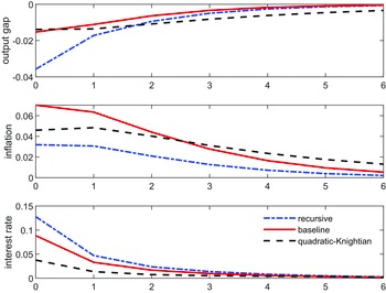
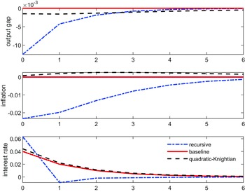
To assess the impact of risk-aversion on the dynamic effects of shocks in the economy, we consider the model described above with both backward- and forward-looking variables, but alternative hypotheses on the central bank’s preferences and type of uncertainty. Thus, we show the impulse-response functions after a one percentage point positive cost-push shock (Figure 1) and a one percentage point positive shock to the natural interest rate (Figure 2) under three different formulations: i) baseline, corresponding to quadratic preferences without Knightian uncertainty on the laws of motion governing the dynamic system (solid line), ii) quadratic-Knightian, corresponding to quadratic preferences with Knightian uncertainty à la Giordani and Söderlind (dashed line), and iii) recursive, corresponding to the case in which the central bank possesses Hansen and Sargent’s recursive preferences but does not face any Knightian uncertainty (dashed-dotted line).
In conducting this analysis we assume that the value of the risk-enhancement coefficient
 $\varrho$
in the formulation with recursive preferences is set equal to 0.05 while in the formulation with Knightian uncertainty-ambiguity aversion is introduced by assuming a Lagrange multiplier
 $\theta$
equal to 20.2.Footnote
16
The latter value is chosen to satisfy the restriction that
 $\theta =1/(\beta \varrho )$
, under which, as indicated in footnote 13, the equivalence between the formulation with Hansen and Sargent’s recursive preferences and that with quadratic preferences and Knightian uncertainty holds in a formulation with backward-looking variables.
Response of output gap, inflation and interest rate to a 1% increase in the cost-push shock
 $\varepsilon _t$
. Solid line: quadratic preferences and no Knightian uncertainty; dashed line: quadratic preferences and Knightian uncertainty à la Giordani and Söderlind; dashed-dotted line: recursive preferences à la Hansen and Sargent. Inflation and interest rate are in annual terms.

Figure 1 shows that for all three formulations a trade-off exists between inflation and output. The inflationary pressures coming from a cost-push shock induce the central bank to respond with a policy that drives output below its efficient level. With the objective of dampening the rise of inflation, the monetary authorities push the output gap to negative values. This policy is called “leaning against the wind”. However, the central bank finds it optimal to accommodate partially the inflationary pressures resulting from the cost-push shock and thus let inflation rise. This increase in inflation is smaller than the increase that it would be observed if the output gap remained unchanged.
Compared to the baseline formulation with quadratic preferences and no Knightian uncertainty, in that with Hansen and Sargent’s recursive preferences we see that the central bank tolerates less an increase in inflation: as a consequence, the interest rate rises more, the recession is higher while inflation increases less. In our simulation, for each percentage point increase in the cost-push shock, the more risk-averse central banker engineers a policy that contracts output twice as much as in the baseline formulation, while inflation is about half the size. In addition, in all three formulations, by increasing the interest rate, the central bank accepts the inflationary pressures only partially. A risk-averse central banker has the lowest tolerance towards the increase in inflation and it accepts a larger contraction in the output gap to reduce the higher inflation brought about by the shock.Footnote 17
Response of output gap, inflation and interest rate to a 1% increase in the demand shock
 $r^n_t$
. Solid line: quadratic preferences and no Knightian uncertainty; dashed line: quadratic preferences and Knightian uncertainty à la Giordani and Söderlind; dashed-dotted line: recursive preferences à la Hansen and Sargent.

In Figure 2 we represent the impulse-response functions after a positive shock to the natural rate, which acts as a demand shock. In the baseline formulation with quadratic preferences and no Knightian uncertainty (solid line) we obtain the standard result according to which the central bank can stabilize the economy by simply moving the interest rate in the same direction and size of the demand shock. On the other hand, in the formulation with Hansen and Sargent’s recursive preferences, a positive demand shock induces a reduction in the output gap and inflation. This occurs because the stronger interest rate response compared to the linear-quadratic formulation breaks the “divine coincidence”, i.e. the possibility to stabilize both of central bank’s targets. Compared to the baseline formulation, the response to the shock by the risk-averse central bank is stronger on impact and weaker after one quarter. Our interpretation is that the central bank follows a risk-management approach, in that it aims at hedging all possible economic fluctuations. This means that it considers the entire covariance matrix of the shocks in setting its policy instrument, coherently with the empirical evidence by Bekaert et al. (Reference Bekaert, Hoerova and Duca2013).
Figures 1 and 2 indicate that a risk-averse central bank sets its monetary policy more aggressively. We corroborate this conclusion simulating the optimal interest rate for values of
 $\varrho$
ranging between 0 and 0.05. We find that the positive relationship between risk-aversion and interest rate setting is monotonic.Footnote
18
The nexus between risk-aversion and monetary policy can also be appreciated by looking at the matrices
 $\mathbf{K}$
and
 $\mathbf{F}$
, which pin down the equilibrium dynamics for the output gap and inflation, and for the interest rate, respectively. Below, we show
 $\mathbf{K}$
and
 $\mathbf{F}$
for the baseline (
 $\varrho = 0$
), recursive (
 $\varrho = 0.05$
) and quadratic-Knightian formulations
 \begin{equation*}\mathbf{K}_{\varrho =0} \, = \, \left [ \begin{array}{cccc} 0.22291 & 0.0007 & 0 & -1.5274 \\ 0.08700 & 0.4791 & 0 & \phantom {-}1.7551 \\ \end{array} \right ] , \end{equation*}
 \begin{equation*}\mathbf{K}_{\varrho =0.05} \, = \, \left [ \begin{array}{cccc} -0.0652 & -0.2058 & -1.2527 & -3.5757 \\ -0.0166 & \phantom {-}0.3863 & -0.5813 & \phantom {-}0.7972 \\ \end{array} \right ] , \end{equation*}
 \begin{equation*}\mathbf{K}_{Knightian} \, = \, \left [ \begin{array}{cccc} 0.216 & -0.0624 & -0.1484 & -1.3862 \\ 0.0635 & 0.4027 & 0.0194 & 1.1481 \\ \end{array} \right ] , \end{equation*}
 \begin{equation*}\mathbf{F}_{\varrho =0} \, = \, \left [ \begin{array}{cccc} 0.45 & 0.23 & 1 & 2.21 \\ \end{array} \right ] , \end{equation*}
 \begin{equation*}\mathbf{F}_{\varrho =0.05} \, = \, \left [ \begin{array}{cccc} 0.66 & 0.33 & 1.6 & 3.19 \\ \end{array} \right ] , \end{equation*}
 \begin{equation*}\mathbf{F}_{Knightian} \, = \, \left [ \begin{array}{cccc} 0.39 & 0.13 & 1.11 & 0.94 \\ \end{array} \right ] . \end{equation*}
The comparison over the values in matrices
 $\mathbf{K}$
and
 $\mathbf{F}$
confirms that the increased convexity of Hansen and Sargent’s preferences changes significantly the transmission of shocks and the monetary policy stance. In particular, the coefficients in
 $\mathbf{F}$
are in absolute terms larger for
 $\varrho = 0.05$
. With Hansen and Sargent’s recursive preferences, the central bank cares about all the shocks that can hit the economy and hence takes into account the covariance matrix
 $\textbf {N}$
with the aim of reducing the uncertainty surrounding the future values of the variables entering the loss function. Indeed, amid a more volatile economic environment –that is with more volatile shocks– we see that the impact of risk-aversion is even more pronounced, in that the central bank becomes even more aggressive.
These results are consistent with conclusions by Vitale (Reference Vitale2018), who establishes within a model with backward-looking variables that a central bank endowed with Hansen and Sargent’s recursive preferences follows a more forceful monetary policy –in particular when operating in a volatile economic environment. This result is related to the extra convexity in the central bank’s preferences introduced in eq. (6). This convexity favors early resolution of uncertainty and leads to an optimal monetary policy which reduces the variability of output and inflation and the monetary authorities’ uncertainty.Footnote 19
If we analyze the policy response to cost-push shocks within the formulations with quadratic preferences, we see that interest rates react more under the baseline formulation. However, this result is not general and it depends on the structure of the model, as shown by Giordani and Söderlind (Reference Giordani and Söderlind2004), and in particular on whether it includes both backward- and forward-looking variables.Footnote 20 Thus, in Section 4.3 we consider a model which only features forward-looking variables and find that the optimal policy with quadratic preferences and Knightian uncertainty is, differently from what we see in Figure 1, more aggressive than that which applies with quadratic preferences and no Knightian uncertainty.
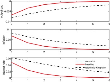
Response of output gap, inflation and interest rate to a 1% increase in the cost-push shock
 $\varepsilon _t$
in a full forward-looking model. Solid line: quadratic preferences and no Knightian uncertainty; dashed line: quadratic preferences and Knightian uncertainty à la Giordani and Söderlind; dashed-dotted line: recursive preferences à la Hansen and Sargent. Inflation and interest rate are in annual terms.

4.3 A formulation without inertia
As argued in Section 3.4, with forward-looking variables, the optimal policy when the policymaker possesses Hansen and Sargent’s recursive preferences and no uncertainty on the laws of motion regulating the dynamics of the state variables is not equivalent to optimal control problems in which the decision maker presents quadratic preferences but faces Knightian uncertainty on the laws of motion. In addition, in our setup risk-aversion matters only if the endogenous variables exhibit inertia and/or the control variables affect the backward-looking variables, while in formulations with forward-looking variables and quadratic preferences, Knightian uncertainty affects the equilibrium independently of the features of the model, as discussed analytically in Appendix C. To emphasize the relevance of the conditions discussed in Section 3.4 under which risk-aversion shapes the optimal policy with forward-looking variables, we consider a version of the model used in the previous simulations where
 $\alpha =\mu =0$
. Under these restrictions the endogenous variables manifest no persistence in their dynamics and the relevance restrictions discussed in Section 3.4 are not met. Figure 3 shows that the central bank’s concern for model misspecification leads to a more aggressive policy (dashed line) without enjoying a better stabilization of output gap and inflation. Moreover, when the model is entirely forward-looking, the optimal policy and the dynamics of inflation and output gap with Hansen and Sargent’s recursive preferences overlap with those which prevail with quadratic preferences and no Knightian uncertainty. This confirms that risk-aversion in the central bank’s preferences calls for a more aggressive policy stance only if the conditions illustrated in Section 3.4 prevail.
5. Concluding remarks
Nowadays central banks need to manage a sizable amount of uncertainty. For this reason their decisions hinge on the degree of risk-aversion of the monetary authorities. This implies that a proper treatment of monetary policy requires to abandon the standard linear-quadratic formulation employed in many theoretical models and consider some risk-adjustment in the objective functions of the monetary authorities, such as that proposed by Epstein and Zin (Reference Epstein and Zin1989) and Hansen and Sargent (Reference Hansen and Sargent1995). Within new Keynesian models introducing such risk- sensitive preferences is challenging, because the central bank needs solving a complex optimal control problem. In this respect, a first contribution of our paper is methodological in that we extend Hansen and Sargent’s (Hansen and Sargent, Reference Hansen and Sargent1995) analysis to models characterized by both backward- and forward-looking variables, as it is often the case in monetary economics.
A second contribution of this paper is then that of investigating the impact of risk-aversion on monetary policy within a workhorse DSGE model proposed by Smets and Wouters (Reference Smets and Wouters2003). We show that a risk-averse central bank conducts a more aggressive policy compared to the policy followed by its risk-neutral counterpart. This occurs because the central bank should consider the variability of shocks that hit the economy, and this breaks the certainty equivalence which applies to the optimal policy within in a linear-quadratic formulation.
A final contribution of this paper has been to show that the equivalence established between risk-sensitive optimal control and robust control by Hansen and Sargent when the dynamic system only contains backward-looking variables no longer applies in the presence of forward-looking ones.
Acknowledgements
A preliminary version of this manuscript was circulated with the title “Risk-sensitive Optimal Control with Forward-looking Variables”. We thank Florina Badarau (editor) and two anonymous referees for the useful comments on the earlier draft.. We thank Barbara Annicchiarico, Jonathan Benchimol, Jérôme Créel, Jean-Cristophe Poutineau, Lorenza Rossi, Louise Schraverus, Mathias Trabandt, all the participants at the
 $1^{st}$
BETA Workshop on DSGE models, at the
 $25^{th}$
INFER Annual Conference and at the
 $28^{th}$
International Conference on Macroeconomic Analysis and International Finance for their comments. We also thank the Editor and two anonymous referees for their advice. The usual disclaimers apply.
Appendix A
Let
 $\mathbf{x}_{1,t} \equiv ( x_{t-1} \ \, \pi _{t-1} \ \, r_{n,t} \ \, \varepsilon _{t} )^{\intercal }$
and
 $\mathbf{x}_{2,t}\equiv (x_{t} \ \, \pi _{t} ) ^{\intercal }$
, and define the matrix
 $\mathbf{A}$
and vector
 $\mathbf{B}$
as follows
 \begin{align*} \mathbf{A} &\equiv \left [ \begin{array}{cccccc} 0 & 0 & 0 & 0 & 1 & 0 \\ 0 & 0 & 0 & 0 & 0 & 1\\ 0 & 0 & \rho _r & 0 & 0 & 0 \\ 0 & 0 & 0 &\rho _{\varepsilon } & 0 & 0 \\ -\frac {\mu }{1-\mu } & \frac {\alpha (1+\alpha )}{\sigma \beta (1+\beta \alpha )(1-\mu )} & -\frac {1}{\sigma (1-\mu )} & \frac {1}{\beta \sigma (1-\mu )(1-\alpha )} & \frac {1}{1-\mu }+\frac {\kappa (1+\alpha )}{\beta \sigma (1-\mu )} &-\frac {1+\alpha }{\beta \sigma (1-\mu )} \\[4pt] 0 &-\frac {\alpha (1+\alpha )}{(1+\beta \alpha )\beta } & 0 & -\frac {1+\alpha }{\beta } & -\frac {\kappa (1+\alpha )}{\beta } & \frac {1+\alpha }{\beta } \end{array} \right ] , \\ \mathbf{B}&\equiv \left [ \begin{array}{c} 0 \\ 0 \\ 0 \\ 0 \\ \frac {1}{\sigma (1-\mu )} \\ 0 \end{array} \right ] . \end{align*}
Then, the vector
 $\mathbf{x}_t^{\intercal } \equiv ( \mathbf{x}_{1,t}^{\intercal } \ \, \mathbf{x}_{2,t}^{\intercal } )$
respects the dynamic system in eq. (5). We can partition matrices
 $\mathbf{A}$
and
 $\mathbf{B}$
as follows
 \begin{align*} \mathbf{A}_{11}&=\left [ \begin{array}{cccc} 0 & 0 & 0 & 0 \\ 0 & 0 &0 &0 \\ 0 & 0 &\rho _{r^n} &0 \\ 0 & 0 &0 &\rho _{\varepsilon } \\ \end{array} \right ] , \nonumber\\ \mathbf{A}_{12}&=\left [ \begin{array}{cc} 1 & 0 \\ 0 & 1 \\ 0 & 0 \\ 0 & 0 \\ \end{array} \right ] ,\nonumber\\ \mathbf{A}_{21}&=\left [ \begin{array}{cccc} -\frac {\mu }{1-\mu } & \frac {\alpha (1+\alpha )}{\sigma \beta (1+\beta \alpha )(1-\mu )} & -\frac {1}{\sigma (1-\mu )} & \frac {1}{\beta \sigma (1-\mu )(1-\alpha )} \\[4pt] 0 &-\frac {\alpha (1+\alpha )}{(1+\beta \alpha )\beta } & 0 & -\frac {1+\alpha }{\beta } \end{array} \right ] , \nonumber\\ \mathbf{A}_{22}&= \left [ \begin{array}{cc} \frac {1}{1-\mu }+\frac {\kappa (1+\alpha )}{\beta \sigma (1-\mu )} &-\frac {1+\alpha }{\beta \sigma (1-\mu )} \\[4pt] -\frac {\kappa (1+\alpha )}{\beta } & \frac {1+\alpha }{\beta } \end{array} \right ] ,\nonumber\\ \mathbf{B}_1^{\intercal } &\equiv \left [ 0 \ \, 0 \ \, 0 \ \, 0 \right ] , \nonumber\\ \mathbf{B}_2^{\intercal } &\equiv \left [ \frac {1}{\sigma (1-\mu )} \ \, 0 \right ] . \end{align*}
In matrix form, the (per-period) cost function defined before
 $c_t = \mathbf{u}_t^{\intercal } \mathbf{Q} \mathbf{u}_t + \mathbf{x}_t^{\intercal } \mathbf{R} \mathbf{x}_t + 2 \mathbf{u}_t^{\intercal } \mathbf{S} \mathbf{x}_t$
here implies that
 $\mathbf{Q}$
and
 $\mathbf{S}$
are zero matrices and
 $\mathbf{R} = \mathbf{C}^{\intercal } \, \Psi \, \mathbf{C}$
, where the matrix
 $\mathbf{C}$
selects a combination of all the variables in the model
 \begin{equation} \left [ \begin{array}{c} x_t-\delta x_{t-1} \\ \pi _t-\alpha \pi _{t-1} \\ \end{array} \right ] = \underbrace {\left [ \begin{array}{ccccccc} -\delta & 0 & 0 & 0 & 1 & 0 \\ 0 & -\alpha & 0 & 0 & 0 & 1 \\ \end{array} \right ]}_{\mathbf{C}} \left [ \begin{array}{c} x_{t-1} \\ \pi _{t-1} \\ r^n_t \\ \epsilon _t \\x_t \\ \pi _t \end{array} \right ] , \quad \Psi = \left [ \begin{array}{cc} \lambda & 0 \\ 0 & 1 \end{array} \right ] , \end{equation}
so that the cost function will be
 $\mathbf{x}_t^{\intercal }\, \mathbf{C}^{\intercal } \, \Psi \, \mathbf{C} \, \mathbf{x}_t$
. Then these matrices can be used to proceed with the derivation in Section 3.
Appendix B
Suppose
 $\boldsymbol{\mathcal{U}}_{t}$
solves Epstein and Zin’s recursion for the following function
 \begin{align*} \boldsymbol{\mathcal{U}}_{t} \ = \ \max \Biggl \{ (1-\beta ) C_t^{1-\xi } \, + \, \beta \, E_t \, \left [ \, \boldsymbol{\mathcal{U}}_{t+1}^{1- \eta } \right ]^{\left(\frac {1-\xi }{1-\eta }\right)} \, \Biggr \}^{\left(\frac {1}{1-\xi }\right)} , \end{align*}
where
 $C_t$
is consumption,
 $\eta$
is the coefficient of relative risk-aversion and
 $1/\xi$
is the elasticity of inter-temporal substitution. Let
 $\xi =1$
. Tallarini (Reference Tallarini2000) shows that
 \begin{align*} \boldsymbol{\mathcal{U}}_{t} \ = \ \max \left \{ C_t^{1-\beta } \, \left ( E_t \, \left [ \boldsymbol{\mathcal{U}}_{t+1}^{1-\eta } \right ] \, \right )^{\left(\frac {\beta }{1-\eta }\right)} \right \} . \end{align*}
Taking logs,
 \begin{align*} \ln \boldsymbol{\mathcal{U}}_{t} \ = \ \max \left \{ (1-\beta ) \, \ln C_t \ + \ \frac {\beta }{1-\eta } \, \ln E_t \, \left [ \boldsymbol{\mathcal{U}}_{t+1}^{1-\eta } \right ] \, \right \} , \end{align*}
or equivalently
 \begin{align*} \frac {\ln \boldsymbol{\mathcal{U}}_{t} }{1-\beta } \ = \ \max \left \{ \, \ln C_t \ + \ \frac {\beta }{(1-\beta )(1-\eta )} \, \ln E_t \, \left [ \boldsymbol{\mathcal{U}}_{t+1}^{1-\eta } \right ] \, \right \} . \end{align*}
We can re-write this as
 \begin{align*} - \frac {\ln \boldsymbol{\mathcal{U}}_{t}}{1-\beta } \ = \ \min \left \{ - \, \ln C_t \ - \ \frac {\beta }{(1-\beta )(1-\eta )} \, \ln E_t \, \left [ \boldsymbol{\mathcal{U}}_{t+1}^{1-\eta } \right ] \, \right \} . \end{align*}
For
 $\boldsymbol{\mathcal{V}}_{t} = - \frac {\ln \boldsymbol{\mathcal{U}}_{t}}{1-\beta }$
, we have that
 $-(1-\beta ) \boldsymbol{\mathcal{V}}_{t} = \ln \boldsymbol{\mathcal{U}}_{t}$
, so that
 $\boldsymbol{\mathcal{U}}_{t+1} = \exp (-(1-\beta ) \boldsymbol{\mathcal{V}}_{t+1} )$
and
 \begin{align*} \boldsymbol{\mathcal{U}}_{t+1}^{1-\eta } \ = \ \left ( \exp (-(1-\beta ) \boldsymbol{\mathcal{V}}_{t+1} ) \right )^{1-\eta } \ = \ \exp (-(1-\beta ) (1-\eta ) \boldsymbol{\mathcal{V}}_{t+1} ) . \end{align*}
Setting
 $\rho ' = -2(1-\beta )(1-\eta )$
, we can write
 \begin{align*} \boldsymbol{\mathcal{V}}_{t} \ = \ \min \left \{ \, - \ln C_t \ + \ \beta \, \frac {2}{\rho '} \, \ln E_t \, \left [ \exp \left ( \frac {\rho '}{2} \boldsymbol{\mathcal{V}}_{t+1} \right ) \right ] \, \right \} , \end{align*}
which corresponds to the value function (6) for
 $\varrho = \frac {\varrho '}{\beta } = 2 \left (\frac {1}{\beta } - 1 \right ) (\eta -1)$
and
 $- \ln C_t$
equal to a quadratic form in the control and state vectors.
Notice that we can invert this relationship and find that
 $\eta = 1 + \frac {1}{2} \left (\frac {\beta }{1-\beta }\, \right ) \varrho$
and that, for
 $\varrho \gt 0$
the coefficient of relative risk-aversion is greater than one.
Appendix C - Risk-sensitive preferences and robust control
Hansen and Sargent (Reference Hansen and Sargent2008) illustrate how the solution to the recursive optimization (6) is equivalent to that of an alternative control problem where only backward-looking variables exist. In particular, consider the case in which the agents are uncertain about the laws of motion describing the dynamics of the state variables. Thus, while they conjecture that the laws of motion are given by the following formulation
 \begin{eqnarray} \mathbf{x}_{t+1} & = & \mathbf{A} \, \mathbf{x}_t \, + \, \mathbf{B} \, \mathbf{u}_t \, + \, \mathbf{C} \, \boldsymbol{\omega }_{t+1} , \end{eqnarray}
representing in the robustness literature the approximating model,Footnote 21 they suspect the actual dynamics for such variables is given by a modified eq., corresponding to the distorted model,
 \begin{eqnarray} \mathbf{x}_{t+1} & = \mathbf{A} \, \mathbf{x}_{t} \ + \ \mathbf{B} \, \mathbf{u}_t \ + \ \mathbf{C} \, ( \boldsymbol{\omega }_{t+1} \, + \, \mathbf{v}_{t+1} ) , \end{eqnarray}
where
 $\mathbf{v}_{t+1}$
is a measurable function of the history of the state vector
 $\mathbf{x}_t$
.
Assuming shocks are normally distributed, the probabilistic distance between the approximating and distorted models, which is an inter-temporal measure of the model misspecification, is
 \begin{eqnarray} \mathcal{R}(\mathbf{v}_{t+1} ) & = & E_t \left [ \sum _{i=1}^{\infty } \, \beta ^i \, \mathbf{v}_{t+i}^{\intercal } \, \mathbf{v}_{t+i} \right ] . \end{eqnarray}
For the same per-period cost used in the main text,
 $c_t = \mathbf{u}_t^{\intercal } \mathbf{Q} \mathbf{u}_t + \mathbf{x}_t^{\intercal } \mathbf{R} \mathbf{x}_t + 2 \mathbf{u}_t^{\intercal } \mathbf{S} \mathbf{x}_t$
, in the corresponding robust control problem in
 $t$
they solve the following constraint problem
 \begin{eqnarray} \min _{\{\mathbf{u}_{t+i}\}_{i=0}^{\infty }} \, \max _{\{ \mathbf{v}_{t+i}\}_{i=1}^{\infty }} \, E_t \left [ \sum _{i=0}^{\infty } \, \beta ^i \, c_{t+i} \right ] , \end{eqnarray}
such that
 $\mathbf{x}_t$
follows the distorted model in eq. (C.2) and the entropy constraint that
 $\mathcal{R}(\mathbf{v}_{t+1} ) \lt \eta _0$
(with
 $\eta _0$
some positive value) is satisfied.
Hansen and Sargent (Reference Hansen and Sargent2008) (Chapter 2.5) show how the decision rule applied by the agents as a solution to the constraint problem (C.4) coincides with that that applies to an optimal control problem where preferences are represented by the recursive optimization (6) and the state variables follow the dynamic laws of motion in eq. (C.1).
The same equivalence result does not hold when the dynamic system involves forward-looking variables. In order to illustrate this point assume that the agents conjecture that the laws of motion are given by eq. (5), while they suspect that they are actually given by the following ones,Footnote 22
 \begin{eqnarray} \left [ \begin{array}{c} \mathbf{x}_{1,t+1} \\ E_t [\mathbf{x}_{2,t+1} ] \end{array} \right ] & = & \mathbf{A} \, \left [ \begin{array}{c} \mathbf{x}_{1,t} \\ \mathbf{x}_{2,t} \end{array} \right ] \ + \ \mathbf{B} \, \mathbf{u}_t \ + \ \left [ \begin{array}{c} \mathbf{C}_1 \left ( \boldsymbol{\omega }_{1,t+1} \, + \, \mathbf{v}_{1,t+1} \right ) \\ \mathbf{0}_{n_2 \times 1} \end{array} \right ] , \end{eqnarray}
where we maintain that
 $\mathbf{C}_1 \boldsymbol{\omega }_{1,t+1} = \boldsymbol{\epsilon }_{1,t+1}$
.
Giordani and Söderlind (Reference Giordani and Söderlind2004) discuss how to solve the constraint control problem (C.4) with forward-looking variables. In particular, they notice, as shown in the original analysis by Hansen and Sargent, that solving the constraint problem (C.4) is equivalent to solving the multiplier problem
 \begin{eqnarray} \min _{\{\mathbf{u}_{t+i}\}_{i=0}^{\infty }} \, \max _{\{ \mathbf{v}_{1,t+i}\}_{i=1}^{\infty }} \, E_t \left [ \sum _{i=0}^{\infty } \, \beta ^i \, ( c_{t+i} \ - \ \theta \, \mathbf{v}_{1,t+i+1}^{\intercal } \mathbf{v}_{1,t+i+1} ) \right ] , \end{eqnarray}
such that
 $\mathbf{x}_t$
follows the distorted model in eq. (C.5), with
 $\theta$
a positive Lagrangian multiplier which subsumes the entropy constraint
 $\mathcal{R}( \mathbf{v}_{1,t+1} ) \lt \eta _0$
. This multiplier model can be re-written in an alternative, more convenient, format as followsFootnote
23
 \begin{eqnarray} \min _{\{\mathbf{u}_{t+i}\}_{i=0}^{\infty }} \, \max _{\{ \mathbf{v}_{1,t+i}\}_{i=0}^{\infty }} \, E_t \left [ \sum _{i=0}^{\infty } \, \beta ^i \, \tilde {c}_{t+i} \right ] , \end{eqnarray}
such that
 $\mathbf{x}_t$
follows the modified distorted model
 \begin{eqnarray} \mathbf{x}_{t+1} & = \mathbf{A} \, \mathbf{x}_{t} \ + \ \widetilde {\mathbf{B}} \, \widetilde {\mathbf{u}}_t \ + \ \mathbf{C} \, \boldsymbol{\omega }_{t+1} , \end{eqnarray}
where
 \begin{eqnarray*} \tilde {c}_t & = & \tilde {\mathbf{u}}_t^{\intercal } \widetilde {\mathbf{Q}} \tilde {\mathbf{u}}_t \, + \, \mathbf{x}_t^{\intercal } \mathbf{R} \mathbf{x}_t \, + \, 2 \tilde {\mathbf{u}}_t^{\intercal } \widetilde {\mathbf{S}} \mathbf{x}_t , \end{eqnarray*}
 \begin{eqnarray*} \widetilde {\mathbf{B}} \ = \ \left [ \begin{array}{cc} \mathbf{B} & \mathbf{C} \end{array} \right ] , & \mathbf{C} \ = \ \left [ \begin{array}{c} \mathbf{C}_1 \\[1ex] \mathbf{0}_{n_{2} \times n_{1}} \end{array} \right ] , & \tilde {\mathbf{u}}_t \ = \ \left [ \begin{array}{c} \mathbf{u}_t \\[1ex] \mathbf{v}_{1,t+1} \end{array} \right ] , \end{eqnarray*}
 \begin{eqnarray*} \widetilde {\mathbf{Q}} \ = \ \left [ \begin{array}{cc} \mathbf{Q} & \mathbf{0}_{k\times n_{1}} \\[1ex] \mathbf{0}_{k\times n_1} & - \theta \mathbf{I}_{n_{1}} \end{array} \right ] & \mbox{and} & \tilde {\mathbf{S}} \ = \ \left [ \begin{array}{cc} \mathbf{S} & \mathbf{0}_{n \times n_{1}} \end{array} \right ] . \end{eqnarray*}
Under the assumption that there exists a matrix
 $\mathbf{K}_t$
such that
 $E_t [\mathbf{x}_{2,t} ] = \mathbf{K}_t \mathbf{x}_{1,t}$
, Giordani and Söderlind (Reference Giordani and Söderlind2004) show that the value function and the robust control of the modified multipier problem (C.7) areFootnote
24
 \begin{align}&\qquad\qquad\qquad\qquad\qquad\quad \boldsymbol{\mathcal{V}}_{t}^R (\mathbf{x}_{1,t}) = \mathbf{x}_{1,t}^{\intercal } \mathbf{V}_t^R \mathbf{x}_{1,t} \, + \, \nu _t , \end{align}
 \begin{align}&\qquad\qquad\qquad\qquad\qquad\qquad \widetilde {\mathbf{u}}_t^* = - \mathbf{F}_t^R \, \mathbf{x}_{1,t} , \ \ \ \mbox{with} \end{align}
 \begin{align}&\qquad\qquad\qquad\qquad\quad\qquad\qquad \mathbf{F}_t^R = \mathbf{\mathcal{F}}_t^R (\mathbf{V}_{t+1}^R) , \end{align}
 \begin{align}&\qquad\qquad\qquad\qquad\qquad\quad\,\, \mathbf{V}_t^R = \mathbf{\mathcal{T}}_t^R (\mathbf{V}_{t+1}^R) , \ \ \mbox{where} \end{align}
 \begin{align}&\qquad\qquad\quad \mathbf{\mathcal{F}}_t^R (\mathbf{W}) = \left ( \widehat {\mathbf{Q}}_t^* \, + \, \beta \widehat {\mathbf{B}}_t^{*^{\intercal }} \mathbf{W} \widehat {\mathbf{B}}_t^*\right )^{-1} \left ( \widehat {\mathbf{S}}_t^{*^\intercal } \, + \, \beta \widehat {\mathbf{B}}_t^{*^{\intercal }}\mathbf{W} \mathbf{A}_t^* \right ) , \end{align}
 \begin{align}& \mathbf{\mathcal{T}}_t^R (\mathbf{W}) = \mathbf{R}_t^* \ - \, 2 \widehat {\mathbf{S}}_t^* \, \mathbf{F}_t^R \, + \, \mathbf{F}_t^{{R}^{\intercal }} \, \widehat {\mathbf{Q}}_t^* \, \mathbf{F}_t^R \, + \, \beta \left (\mathbf{A}_t^* \, - \, \widehat {\mathbf{B}}_t^* \mathbf{F}_t^R \right )^{\intercal } \mathbf{W} \left (\mathbf{A}_t^* \, - \, \widehat {\mathbf{B}}_t ^*\mathbf{F}_t^R \right ) , \end{align}
 \begin{eqnarray*} \widehat {\mathbf{B}}_t^* & = & \widetilde {\mathbf{B}}_{1} \ + \ \mathbf{A}_{12} \, \widehat {\mathbf{G}}_t^* , \\[1ex] \widehat {\mathbf{G}}_t^* & = & ( \mathbf{A}_{22} \, - \, \mathbf{K}_{t+1} \mathbf{A}_{12})^{-1} (\mathbf{K}_{t+1} \widetilde {\mathbf{B}}_{1} \, - \, \widetilde {\mathbf{B}}_{2}) , \\[1ex] \widehat {\mathbf{S}}_t^* & = & \mathbf{D}_t^{\intercal } \, \mathbf{R}_{22} \, \widehat {\mathbf{G}}_t^* \, + \, \mathbf{R}_{12}\, \widehat {\mathbf{G}}_t^* \, + \, \widetilde {\mathbf{S}}_{1} \, + \, \mathbf{D_t}^{\intercal } \, \widetilde {\mathbf{S}}_{2} , \\[1ex] \widehat {\mathbf{Q}}_t^* & = & \widehat {\mathbf{G}}_t^{*^\intercal } \, \mathbf{R}_{22} \, \widehat {\mathbf{G}}_t^* \, + \, 2\, \widehat {\mathbf{G}}_t^{*^\intercal } \, \widetilde {\mathbf{S}}_{2} \, + \, \widetilde {\mathbf{Q}} \, \end{eqnarray*}
and
 \begin{eqnarray*} \widetilde {\mathbf{S}} & = & \left [ \begin{array}{c} \widetilde {\mathbf{S}}_1 \\[1ex] \widetilde {\mathbf{S}}_2 \end{array} \right ] . \end{eqnarray*}
Importantly, we notice that for any choice of the matrices
 $\mathbf{B}_1$
and
 $\mathbf{A}_{12}$
the matrix
 $\mathbf{F}_t^R$
depends on
 $\theta$
via
 $\widehat {\mathbf{Q}}_t^*$
. This implies that under those circumstances, namely
 $\mathbf{B}_1=\mathbf{0}$
and
 $\mathbf{A}_{12} =\mathbf{0}$
, under which risk-aversion does not influence the optimal policy, as illustrated in Section 3.4, Knightian uncertainty conditions the robust policy. This implies that in the presence of forward-looking variables, the optimal policy in the formulation with Hansen and Sargent’s recursive preferences does not correspond to the robust policy selected by an agent facing Knightian uncertainty and endowed with standard quadratic preferences.