2. Formulation of the problem

Consider a mixture of smooth hard spheres, composed of species $A$ and $B$ , of mass $m_{A}$ and $m_{B}$ , and diameters $d_{A}$ and $d_{B}$ . The decay of kinetic energy in a collision is characterized by a coefficient of normal restitution $e$ , assumed to be independent of the initial normal relative velocity, defined as the ratio between the postcollisional and precollisional normal relative velocity of the colliding spheres.

The transformation of velocities in a collision between sphere $A$ and sphere $B$ reads:

(2.1) $$\begin{eqnarray}\displaystyle \left.\begin{array}{@{}c@{}}\displaystyle \boldsymbol{v}_{1}=\boldsymbol{v}_{1}^{\prime }-(1+e)M^{BA}(\boldsymbol{k}\boldsymbol{\cdot }\boldsymbol{v}_{12}^{\prime })\boldsymbol{k},\\ \displaystyle \boldsymbol{v}_{2}=\boldsymbol{v}_{2}^{\prime }+(1+e)M^{AB}(\boldsymbol{k}\boldsymbol{\cdot }\boldsymbol{v}_{12}^{\prime })\boldsymbol{k},\end{array}\!\!\right\} & & \displaystyle\end{eqnarray}$$

where $M^{{\it\alpha}{\it\beta}}\equiv m_{{\it\alpha}}/(m_{{\it\alpha}}+m_{{\it\beta}})$ for $\{{\it\alpha},{\it\beta}\}\in \{A,B\}$ , primes denote precollisional velocities, the indices ‘ $1$ ’ and ‘ $2$ ’ pertain here to the species $A$ and $B$ , respectively, $\boldsymbol{v}_{12}\equiv \boldsymbol{v}_{1}-\boldsymbol{v}_{2}$ and $\boldsymbol{k}$ is a unit vector pointing from the centre of sphere $A$ to that of sphere $B$ . The standard description of binary mixtures of inelastic gases involves three coefficients of restitution, one for each type of collision. In the case of fluctuating coefficient of restitution, these have to be replaced by three distributions for $e$ , denoted here ${\it\rho}_{AA}(e)$ , ${\it\rho}_{AB}(e)$ , and ${\it\rho}_{BB}(e)$ . The kinetic description of a binary mixture of dilute gas requires two distribution functions, $f_{A}(\boldsymbol{v},\boldsymbol{r},t)$ and $f_{B}(\boldsymbol{v},\boldsymbol{r},t)$ . Their dynamics is described by a set of two coupled Boltzmann equations:

(2.2) $$\begin{eqnarray}\mathscr{D}f_{{\it\alpha}}\equiv \frac{\partial f_{{\it\alpha}}}{\partial t}+\boldsymbol{v}_{1}\boldsymbol{\cdot }\boldsymbol{{\rm\nabla}}f_{{\it\alpha}}=\mathscr{B}_{{\it\alpha}{\it\alpha}}(\,f_{{\it\alpha}},f_{{\it\alpha}},{\it\rho}_{{\it\alpha}{\it\alpha}})+\mathscr{B}_{{\it\alpha}{\it\beta}}(\,f_{{\it\alpha}},f_{{\it\beta}},{\it\rho}_{{\it\alpha}{\it\beta}}),\end{eqnarray}$$

for $\{{\it\alpha},{\it\beta}\}\in \{A,B\}$ , with ${\it\alpha}\not ={\it\beta}$ . The Boltzmann operator $\mathscr{B}_{{\it\alpha}{\it\beta}}(\,f_{{\it\alpha}},f_{{\it\beta}},{\it\rho}_{{\it\alpha}{\it\beta}})$ corresponding to ${\it\alpha}$ – ${\it\beta}$ collisions in the case of (impact velocity independent) stochastic coefficient of restitution is a generalization of that defined for mixtures of gas interacting with constant coefficients of restitution (Chapman & Cowling Reference Chapman and Cowling1970). Its dependence on the coefficient of restitution is modified to include a functional dependence on the distributions ${\it\rho}_{{\it\alpha}{\it\beta}}(e)$ for the coefficients of restitution, corresponding to an average over the values of $e$ , with a weight given by ${\it\rho}_{{\it\alpha}{\it\beta}}(e)$ :

(2.3) $$\begin{eqnarray}\displaystyle \mathscr{B}_{{\it\alpha}{\it\beta}}(\,f_{{\it\alpha}},f_{{\it\beta}},{\it\rho}_{{\it\alpha}{\it\beta}}) & = & \displaystyle d_{{\it\alpha}{\it\beta}}^{2}\iiint _{\boldsymbol{v}_{12}\boldsymbol{\cdot }\boldsymbol{k}>0}{\it\rho}_{{\it\alpha}{\it\beta}}(e)\left[\frac{f_{{\it\alpha}}(\boldsymbol{v}_{1}^{\prime })f_{{\it\beta}}(\boldsymbol{v}_{2}^{\prime })}{e^{2}}-f_{{\it\alpha}}(\boldsymbol{v}_{1})f_{{\it\beta}}(\boldsymbol{v}_{2})\right]\nonumber\\ \displaystyle & & \displaystyle \times \,(\boldsymbol{v}_{12}\boldsymbol{\cdot }\boldsymbol{k})\,\text{d}\boldsymbol{v}_{2}\,\text{d}\boldsymbol{k}\,\text{d}e,\end{eqnarray}$$

where $d_{{\it\alpha}{\it\beta}}\equiv (d_{{\it\alpha}}+d_{{\it\beta}})/2$ . Here $\boldsymbol{v}_{1}$ and $\boldsymbol{v}_{1}^{\prime }$ pertain to species ${\it\alpha}$ , and $\boldsymbol{v}_{2}$ and $\boldsymbol{v}_{2}^{\prime }$ pertain to ${\it\beta}$ . From a hydrodynamic point of view, the system is described by a set of fields corresponding to averages of the conserved quantities in collisions, namely the two number densities $n_{A}$ and $n_{B}$ (or alternatively the total number density $n\equiv n_{A}+n_{B}$ and the concentration $c\equiv n_{A}/n$ of species $A$ ), the velocity $\boldsymbol{V}$ (or momentum density), which is defined as a mass average of the species’ mean velocities and the temperature field, $T$ , defined as (twice) the mean fluctuating kinetic energy of a fluid particle. Notice that in the case of inelastic gases, the temperature is not a proper hydrodynamic field as it corresponds to the mean kinetic energy which is dissipated in collisions. The hydrodynamic fields can be expressed in terms of the distribution function the following way: the number density for species ${\it\alpha}$ is given by:

(2.4) $$\begin{eqnarray}n_{{\it\alpha}}=\int f_{{\it\alpha}}(\boldsymbol{v})\,\text{d}\boldsymbol{v},\end{eqnarray}$$

the corresponding mass density being ${\it\rho}_{m_{{\it\alpha}}}=m_{{\it\alpha}}n_{{\it\alpha}}$ . The overall number density is $n=n_{A}+n_{B}$ , and the overall mass density is ${\it\rho}_{m}\equiv {\it\rho}_{m_{A}}+{\it\rho}_{m_{B}}$ . The mixture’s velocity field is:

(2.5) $$\begin{eqnarray}\boldsymbol{V}=\frac{1}{{\it\rho}_{m}}({\it\rho}_{m_{A}}\boldsymbol{V}_{A}+{\it\rho}_{m_{B}}\boldsymbol{V}_{B}),\end{eqnarray}$$

where $\boldsymbol{V}_{{\it\alpha}}$ is the velocity field of species ${\it\alpha}$ , given by:

(2.6) $$\begin{eqnarray}\boldsymbol{V}_{{\it\alpha}}=\frac{1}{n_{{\it\alpha}}}\int f_{{\it\alpha}}(\boldsymbol{v})\boldsymbol{v}\,\text{d}\boldsymbol{v}.\end{eqnarray}$$

$\boldsymbol{V}_{{\it\alpha}}$ is not a hydrodynamic field and needs to be expressed as a function of the hydrodynamic fields. The same holds for the granular temperature of species ${\it\alpha}$ , defined by:

(2.7) $$\begin{eqnarray}T_{{\it\alpha}}=\frac{1}{n_{{\it\alpha}}}\int f_{{\it\alpha}}(\boldsymbol{v})m_{{\it\alpha}}(\boldsymbol{v}-\boldsymbol{V})^{2}\,\text{d}\boldsymbol{v}.\end{eqnarray}$$

The mixture’s granular temperature (average fluctuating kinetic energy multiplied by 2) is defined by:

(2.8) $$\begin{eqnarray}T\equiv \frac{1}{n}(n_{A}T_{A}+n_{B}T_{B}).\end{eqnarray}$$

As mentioned above, the temperature is not a proper hydrodynamic field since it corresponds to the (internal) kinetic energy of the particles, which is not conserved in collisions, and therefore does not qualify as a ‘slow field’. It is however an important characterization of the state of a granular gas (Goldhirsch Reference Goldhirsch2003) and it can be shown that it has to be included in a hydrodynamic description (Dufty & Brey Reference Dufty and Brey2011).

The equations of motion for the hydrodynamic fields can be readily obtained upon considering moments of the Boltzmann equations (although their validity is not restricted to the range of validity of the latter). Multiplying the Boltzmann equations by $1,$ $m_{{\it\alpha}}\boldsymbol{v}$ , and $m_{{\it\alpha}}u^{2}$ , integrating and summing over the species provides kinetic expressions for the particle flux densities, stress tensor and heat flux. The equation of motion for the number density, $n_{{\it\alpha}}$ , with ${\it\alpha}\in \{A,B\}$ , is obtained by integrating (2.2) over velocities:

(2.9) $$\begin{eqnarray}\frac{\text{D}n_{{\it\alpha}}}{\text{D}t}=-\text{div}\,\boldsymbol{J}_{{\it\alpha}}-n_{{\it\alpha}}\text{div}\,\boldsymbol{V},\end{eqnarray}$$

where $\text{D}/\text{D}t=\partial /\partial t+\boldsymbol{V}\boldsymbol{\cdot }\boldsymbol{{\rm\nabla}}$ is the material derivative and

(2.10) $$\begin{eqnarray}\boldsymbol{J}_{{\it\alpha}}=n_{{\it\alpha}}(\boldsymbol{V}_{{\it\alpha}}-\boldsymbol{V}),\end{eqnarray}$$

is the particle flux density of species ${\it\alpha}$ . As $\boldsymbol{V}_{{\it\alpha}}$ , the velocity field of species ${\it\alpha}$ , or equivalently the flux, $\boldsymbol{J}_{{\it\alpha}}$ , is not a hydrodynamic field and must be given by an appropriate constitutive relation. The equation of motion obeyed by the velocity field (in the absence of an external force) can be written in the following standard form, obtained by multiplying (2.2) by $m_{{\it\alpha}}\boldsymbol{v}$ , integrating on velocities and summing over the two species:

(2.11) $$\begin{eqnarray}{\it\rho}_{m}\frac{\text{D}V_{i}}{\text{D}t}=-\frac{\partial \unicode[STIX]{x1D617}_{ij}}{\partial x_{j}}.\end{eqnarray}$$

The kinetic expression for the stress tensor (in the dilute case, which excludes the collisional contribution) is given by:

(2.12) $$\begin{eqnarray}\unicode[STIX]{x1D617}_{ij}=m_{A}\int f_{A}(\boldsymbol{v})u_{i}u_{j}\,\text{d}\boldsymbol{v}+m_{B}\int f_{B}(\boldsymbol{v})u_{i}u_{j}\,\text{d}\boldsymbol{v},\end{eqnarray}$$

where $\boldsymbol{u}\equiv \boldsymbol{v}-\boldsymbol{V}$ is the peculiar (fluctuating) velocity. The granular temperature field obeys the equation of motion (obtained by integrating (2.2) multiplied by $m_{{\it\alpha}}u^{2}$ and summing the contributions of the two species), and reads:

(2.13) $$\begin{eqnarray}n\frac{\text{D}T}{\text{D}t}=T\text{div}\,\boldsymbol{J}-\text{div}\,\boldsymbol{Q}-2\unicode[STIX]{x1D617}_{ij}\frac{\partial V_{i}}{\partial x_{j}}-{\it\Gamma},\end{eqnarray}$$

where $\boldsymbol{J}\equiv \boldsymbol{J}_{A}+\boldsymbol{J}_{B}$ is the total particle flux, $Q$ is the heat flux given by:

(2.14) $$\begin{eqnarray}\boldsymbol{Q}=\int f_{A}(\boldsymbol{v})m_{A}u^{2}\boldsymbol{u}\,\text{d}\boldsymbol{v}+\int f_{B}(\boldsymbol{v})m_{B}u^{2}\boldsymbol{u}\,\text{d}\boldsymbol{v}\end{eqnarray}$$

and ${\it\Gamma}$ is the energy sink term, which accounts for the rate of loss of energy due to the inelasticity of the collisions (and therefore vanishes in the elastic limit). It is given by:

(2.15) $$\begin{eqnarray}{\it\Gamma}={\it\Gamma}_{A}+{\it\Gamma}_{B}+{\it\Gamma}_{AB}.\end{eqnarray}$$

The contributions to ${\it\Gamma}$ are:

(2.16) $$\begin{eqnarray}{\it\Gamma}_{{\it\alpha}}\equiv \iiint {\it\rho}_{{\it\alpha}{\it\alpha}}(e)\frac{(1-e^{2})m_{{\it\alpha}}}{8}{\rm\pi}d_{{\it\alpha}}^{2}f_{{\it\alpha}}(\boldsymbol{v}_{1})f_{{\it\alpha}}(\boldsymbol{v}_{2})|\boldsymbol{v}_{12}|^{3}\,\text{d}\boldsymbol{v}_{1}\,\text{d}\boldsymbol{v}_{2}\,\text{d}e,\end{eqnarray}$$

and

(2.17) $$\begin{eqnarray}{\it\Gamma}_{AB}\equiv \iiint {\it\rho}_{AB}(e)\frac{(1-e^{2})m_{AB}{\rm\pi}\,d_{AB}^{2}}{2}f_{A}(\boldsymbol{v}_{1})f_{B}(\boldsymbol{v}_{2})|\boldsymbol{v}_{12}|^{3}\,\text{d}\boldsymbol{v}_{1}\,\text{d}\boldsymbol{v}_{2}\,\text{d}e,\end{eqnarray}$$

where $m_{AB}\equiv (m_{A}m_{B})/(m_{A}+m_{B})$ is the reduced mass and $d_{AB}=(d_{A}+d_{B})/2$ .

3. Constitutive relations and transport coefficients

3.1. The Chapman–Enskog (CE) expansion

In order to derive the constitutive relation for the fluxes (2.10), (2.12), (2.14) and the sources (2.15), we proceed to solve (2.2) by performing a Chapman–Enskog expansion. The latter consists in a perturbative gradient expansion of the distribution function (formally in powers of the Knudsen number) around a reference state corresponding to a homogeneous solution of the Boltzmann equation (the Maxwellian equilibrium distribution function for elastic systems, $f_{{\it\alpha}}^{M}=n_{{\it\alpha}}({\it\gamma}_{{\it\alpha}}/{\rm\pi})^{3/2}\text{e}^{-{\it\gamma}_{{\it\alpha}}u^{2}}$ , with ${\it\gamma}_{{\it\alpha}}\equiv 3m_{{\it\alpha}}/2T$ , or the distribution function corresponding to the homogeneous cooling state in the present case (Brey et al. Reference Brey, Dufty, Kim and Santos1998), see below). The distribution function is thus written:

(3.1) $$\begin{eqnarray}f_{{\it\alpha}}\equiv f_{{\it\alpha}}^{M}{\it\phi}_{{\it\alpha}}=f_{{\it\alpha}}^{M}({\it\phi}_{{\it\alpha}}^{(0)}+{\it\phi}_{{\it\alpha}}^{K}+{\it\phi}_{{\it\alpha}}^{K^{2}}+\cdots \,),\end{eqnarray}$$

where ${\it\phi}_{{\it\alpha}}$ denotes the correction to the Maxwellian elastic equilibrium distribution and the superscripts denote the order of each term in gradient expansion. In addition to assuming small gradients (or more precisely, Knudsen numbers), the CE method relies on the assumption that the dependence of the distribution function in space and time is implicit through its functional dependence on the fields and that there is no additional space or time dependence, defining a ‘normal solution’ of the Boltzmann equations. In the current case, the pertinent hydrodynamic fields are $n$ , $c\equiv n_{A}/n$ (or alternatively $n_{A}$ and $n_{B}$ ), $\boldsymbol{V}$ , and $T$ , so that the time derivative $\mathscr{D}f$ in (2.2) can be written:

(3.2) $$\begin{eqnarray}\mathscr{D}f_{{\it\alpha}}={\it\phi}_{{\it\alpha}}f_{{\it\alpha}}^{M}[\mathscr{D}\ln n_{{\it\alpha}}+2{\it\gamma}_{{\it\alpha}}u_{i}\mathscr{D}V_{i}+({\it\gamma}_{{\it\alpha}}u^{2}-{\textstyle \frac{3}{2}})\mathscr{D}\ln T]+f_{{\it\alpha}}^{M}\mathscr{D}{\it\phi}_{{\it\alpha}}.\end{eqnarray}$$

The result of the application of the operator $\mathscr{D}$ on any functional of the hydrodynamic fields can thus be in turn expanded in powers of gradients, by making use of the hydrodynamic equations, (2.9), (2.11), (2.13): $\mathscr{D}f=\mathscr{D}^{(0)}f+\mathscr{D}^{K}f+\cdots \,,$ where the subscript identifies the order in expansion. Upon substituting (3.1) and the expansion of $\mathscr{D}f$ in (2.2), and equating the terms of the same order in expansion on both sides of the equation, one obtains a hierarchy of equations.

3.1.1. Zeroth order correction: the homogeneous cooling state

The homogeneous cooling state (HCS) of a granular gas is defined as a state of vanishing velocity and homogeneous density fields. Considering normal solutions, the distribution functions are rendered ‘time independent’ by scaling the velocities by the thermal speed of the species comprising the mixture, i.e. the distribution is assumed to depend on velocity through the variable ${\it\gamma}_{{\it\alpha}}u^{2}$ . Since all gradients vanish in this state, the corresponding distribution function can be taken as the zeroth order in the CE expansion. Using (2.9), (2.11) and (2.13), one has: $\mathscr{D}^{(0)}\ln n_{{\it\alpha}}=0$ , $\mathscr{D}^{(0)}V_{i}=0$ , and $\mathscr{D}^{(0)}\ln T=-{\it\Gamma}/nT$ . The zeroth order of (3.2) therefore reads:

(3.3) $$\begin{eqnarray}\displaystyle \mathscr{D}^{(0)}f_{{\it\alpha}}=-f_{{\it\alpha}}^{M}\left({\it\gamma}_{{\it\alpha}}u^{2}({\it\phi}_{{\it\alpha}}^{(0)}-{\it\phi}_{{\it\alpha}}^{(0)\prime })-\frac{3}{2}{\it\phi}_{{\it\alpha}}^{(0)}\right)\frac{{\it\Gamma}}{nT}, & & \displaystyle\end{eqnarray}$$

where prime denotes a derivative with respect to ${\it\gamma}_{{\it\alpha}}u^{2}$ . The temperature dependence of ${\it\phi}^{(0)}$ , through its argument ${\it\gamma}_{{\it\alpha}}u^{2}$ , has been taken into account. The two coupled Boltzmann equations (2.2) reduce to the following equations for the corrections ${\it\phi}_{{\it\alpha}}^{(0)}$ :

(3.4) $$\begin{eqnarray}\displaystyle -f_{{\it\alpha}}^{M}\left({\it\gamma}_{{\it\alpha}}u^{2}({\it\phi}_{{\it\alpha}}^{(0)}-{\it\phi}_{{\it\alpha}}^{(0)\prime })-\frac{3}{2}{\it\phi}_{{\it\alpha}}^{(0)}\right)\frac{{\it\Gamma}}{nT} & = & \displaystyle \int \mathscr{B}_{{\it\alpha}{\it\alpha}}(f_{{\it\alpha}}^{M}{\it\phi}_{{\it\alpha}}^{(0)},f_{{\it\alpha}}^{M}{\it\phi}_{{\it\alpha}}^{(0)},{\it\rho}_{{\it\alpha}{\it\alpha}}(e),e)\,\text{d}e\nonumber\\ \displaystyle & & \displaystyle +\,\int \mathscr{B}_{{\it\alpha}{\it\beta}}(f_{{\it\alpha}}^{M}{\it\phi}_{{\it\alpha}}^{(0)},f_{{\it\beta}}^{M}{\it\phi}_{{\it\beta}}^{(0)},{\it\rho}_{{\it\alpha}{\it\beta}}(e),e)\,\text{d}e,\nonumber\\ \displaystyle & & \displaystyle\end{eqnarray}$$

where the Boltzmann operator $\mathscr{B}_{{\it\alpha}{\it\beta}}$ is defined in (2.3). These equations need to be solved subject to the following constraints:

(3.5) $$\begin{eqnarray}\displaystyle & \displaystyle \int f_{A}\,\text{d}\boldsymbol{u}=n_{A} & \displaystyle\end{eqnarray}$$

(3.6) $$\begin{eqnarray}\displaystyle & \displaystyle \int f_{B}\,\text{d}\boldsymbol{u}=n_{B} & \displaystyle\end{eqnarray}$$

(3.7) $$\begin{eqnarray}\displaystyle & \displaystyle \int f_{A}m_{A}u^{2}\,\text{d}\boldsymbol{u}+\int f_{B}m_{B}u^{2}\,\text{d}\boldsymbol{u}=nT, & \displaystyle\end{eqnarray}$$

which express the fact that the two number densities and the temperature field have to be given by the appropriate moment of the distribution function.

3.1.2. First-order correction

Computing the transport coefficients to Navier–Stokes order requires calculating the correction ${\it\phi}_{{\it\alpha}}^{K}$ corresponding to the first order in gradient. Carrying out the procedure described above to first order, one obtains the following expression for ${\it\phi}_{{\it\alpha}}^{K}$ (appendix A provides details of the derivation):

(3.8) $$\begin{eqnarray}\displaystyle {\it\phi}_{{\it\alpha}}^{K} & = & \displaystyle {\it\Phi}_{{\it\alpha}}^{K,T}({\it\gamma}_{{\it\alpha}}u^{2})\sqrt{{\it\gamma}_{{\it\alpha}}}\boldsymbol{u}\boldsymbol{\cdot }\boldsymbol{{\rm\nabla}}\ln T+{\it\Phi}_{{\it\alpha}}^{K,n}({\it\gamma}_{{\it\alpha}}u^{2})\sqrt{{\it\gamma}_{{\it\alpha}}}\boldsymbol{u}\boldsymbol{\cdot }\boldsymbol{{\rm\nabla}}\ln n\nonumber\\ \displaystyle & & \displaystyle +\,{\it\Phi}_{{\it\alpha}}^{K,c}({\it\gamma}_{{\it\alpha}}u^{2})\sqrt{{\it\gamma}_{{\it\alpha}}}\boldsymbol{u}\boldsymbol{\cdot }\boldsymbol{{\rm\nabla}}\ln c+{\it\Phi}_{{\it\alpha}}^{K,V}({\it\gamma}_{{\it\alpha}}u^{2}){\it\gamma}_{{\it\alpha}}^{3/2}\overline{\boldsymbol{u}\boldsymbol{u}}\boldsymbol{ : }\boldsymbol{{\rm\nabla}}\boldsymbol{V},\end{eqnarray}$$

where overbar denotes the traceless symmetric part of any second rank tensor, $\unicode[STIX]{x1D63C}\boldsymbol{ : }\overline{\unicode[STIX]{x1D608}_{ij}}\equiv (\unicode[STIX]{x1D608}_{ij}+\unicode[STIX]{x1D608}_{ji}-(2/3){\it\delta}_{ij}\unicode[STIX]{x1D608}_{kk})/2$ , and the functions ${\it\Phi}_{{\it\alpha}}^{K,T},{\it\Phi}_{{\it\alpha}}^{K,c}$ , ${\it\Phi}_{{\it\alpha}}^{K,n}$ and ${\it\Phi}_{{\it\alpha}}^{K,V}$ are isotropic functions of the rescaled peculiar velocity ${\it\gamma}_{{\it\alpha}}u^{2}$ , and obey the following set of equations:

The function ${\it\Phi}_{{\it\alpha}}^{K,V}$ obeys:

(3.9) $$\begin{eqnarray}\displaystyle & & \displaystyle (L_{{\it\alpha}{\it\alpha}}^{(1)}+L_{{\it\alpha}{\it\alpha}}^{(2)}+L_{{\it\alpha}{\it\beta}}^{(1)})\{{\it\Phi}_{{\it\alpha}}^{K,V}({\it\gamma}_{{\it\alpha}}u^{2}){\it\gamma}_{{\it\alpha}}^{3/2}\overline{\boldsymbol{u}\boldsymbol{u}}\}+L_{{\it\alpha}{\it\beta}}^{(2)}\{{\it\Phi}_{{\it\beta}}^{K,V}({\it\gamma}_{{\it\beta}}u^{2}){\it\gamma}_{{\it\beta}}^{3/2}\overline{\boldsymbol{u}\boldsymbol{u}}\}\nonumber\\ \displaystyle & & \displaystyle \qquad -\,\frac{\sqrt{6{\rm\pi}}}{9}\frac{nd_{{\it\alpha}{\it\beta}}^{2}}{\sqrt{m_{0}}}\widetilde{{\it\Gamma}}\sqrt{T}f_{{\it\alpha}}^{M}((\mathscr{H}\{{\it\Phi}_{{\it\alpha}}^{K,V}\}+3){\it\Phi}_{{\it\alpha}}^{K,V}({\it\gamma}_{{\it\alpha}}u^{2}){\it\gamma}_{{\it\alpha}}^{3/2}\overline{\boldsymbol{u}\boldsymbol{u}})\nonumber\\ \displaystyle & & \displaystyle \quad =2f_{{\it\alpha}}^{M}{\it\gamma}_{{\it\alpha}}({\it\phi}_{{\it\alpha}}^{(0)}-{\it\phi}_{{\it\alpha}}^{(0)\prime })\overline{\boldsymbol{u}\boldsymbol{u}},\end{eqnarray}$$

where $m_{0}\equiv m_{A}+m_{B}$ , and $\tilde{{\it\Gamma}}\equiv (9/\sqrt{6{\rm\pi}})(\sqrt{m_{0}}/(n^{2}d_{AB}^{2}T^{3/2})){\it\Gamma}$ , the function ${\it\Phi}_{{\it\alpha}}^{K,T}$ obeys:

(3.10) $$\begin{eqnarray}\displaystyle & & \displaystyle (L_{{\it\alpha}{\it\alpha}}^{(1)}+L_{{\it\alpha}{\it\alpha}}^{(2)}+L_{{\it\alpha}{\it\beta}}^{(1)})\{{\it\Phi}_{{\it\alpha}}^{K,T}({\it\gamma}_{{\it\alpha}}u^{2})\sqrt{{\it\gamma}_{{\it\alpha}}}\boldsymbol{u}\}+L_{{\it\alpha}{\it\beta}}^{(2)}\{{\it\Phi}_{{\it\beta}}^{K,T}({\it\gamma}_{{\it\beta}}u^{2})\sqrt{{\it\gamma}_{{\it\beta}}}\boldsymbol{u}\}\nonumber\\ \displaystyle & & \displaystyle \qquad -\,\frac{\sqrt{6{\rm\pi}}}{9}\frac{nd_{{\it\alpha}{\it\beta}}^{2}}{\sqrt{m_{0}}}\widetilde{{\it\Gamma}}\sqrt{T}f_{{\it\alpha}}^{M}\left(\left(\mathscr{H}\{{\it\Phi}_{{\it\alpha}}^{K,T}\}+\frac{3}{4}\right){\it\Phi}_{{\it\alpha}}^{K,T}({\it\gamma}_{{\it\alpha}}u^{2})\sqrt{{\it\gamma}_{{\it\alpha}}}\boldsymbol{u}\right)\nonumber\\ \displaystyle & & \displaystyle \quad =f_{{\it\alpha}}^{M}\left(\left({\it\gamma}_{{\it\alpha}}u^{2}-\frac{nm_{{\it\alpha}}}{{\it\rho}_{m}}\right)({\it\phi}_{{\it\alpha}}^{(0)}-{\it\phi}_{{\it\alpha}}^{(0)\prime })-\frac{3}{2}{\it\phi}_{{\it\alpha}}^{(0)}\right)\boldsymbol{u},\end{eqnarray}$$

the function ${\it\Phi}_{{\it\alpha}}^{K,n}$ obeys:

(3.11) $$\begin{eqnarray}\displaystyle & & \displaystyle (L_{{\it\alpha}{\it\alpha}}^{(1)}+L_{{\it\alpha}{\it\alpha}}^{(2)}+L_{{\it\alpha}{\it\beta}}^{(1)})\{{\it\Phi}_{{\it\alpha}}^{K,n}({\it\gamma}_{{\it\alpha}}u^{2})\sqrt{{\it\gamma}_{{\it\alpha}}}\boldsymbol{u}\}+L_{{\it\alpha}{\it\beta}}^{(2)}\{{\it\Phi}_{{\it\beta}}^{K,n}({\it\gamma}_{{\it\beta}}u^{2})\sqrt{{\it\gamma}_{{\it\beta}}}\boldsymbol{u}\}\nonumber\\ \displaystyle & & \displaystyle \qquad -\,\frac{\sqrt{6{\rm\pi}}}{9}\frac{nd_{{\it\alpha}{\it\beta}}^{2}}{\sqrt{m_{0}}}\widetilde{{\it\Gamma}}\sqrt{T}f_{{\it\alpha}}^{M}((\mathscr{H}\{{\it\Phi}_{{\it\alpha}}^{K,n}\}+2){\it\Phi}_{{\it\alpha}}^{K,n}({\it\gamma}_{{\it\alpha}}u^{2})\sqrt{{\it\gamma}_{{\it\alpha}}}\boldsymbol{u}-{\it\Phi}_{{\it\alpha}}^{K,T}({\it\gamma}_{{\it\alpha}}u^{2})\sqrt{{\it\gamma}_{{\it\alpha}}}\boldsymbol{u})\nonumber\\ \displaystyle & & \displaystyle \quad =f_{{\it\alpha}}^{M}\left({\it\phi}_{{\it\alpha}}^{(0)}-\frac{nm_{{\it\alpha}}}{{\it\rho}_{m}}({\it\phi}_{{\it\alpha}}^{(0)}-{\it\phi}_{{\it\alpha}}^{(0)\prime })\right)\boldsymbol{u},\end{eqnarray}$$

for $\{{\it\alpha},{\it\beta}\}\in \{A,B\}$ , with ${\it\alpha}\not ={\it\beta}$ . The function ${\it\Phi}_{A}^{K,c}$ obeys:

(3.12) $$\begin{eqnarray}\displaystyle & & \displaystyle (L_{AA}^{(1)}+L_{AA}^{(2)}+L_{AA}^{(1)})\{{\it\Phi}_{A}^{K,c}({\it\gamma}_{A}u^{2})\sqrt{{\it\gamma}_{B}}\boldsymbol{u}\}+L_{AB}^{(2)}\{{\it\Phi}_{B}^{K,c}({\it\gamma}_{B}u^{2})\sqrt{{\it\gamma}_{B}}\boldsymbol{u}\}-\frac{\sqrt{6{\rm\pi}}}{9}\frac{nd_{AB}^{2}}{\sqrt{m_{0}}}\widetilde{{\it\Gamma}}\sqrt{T}f_{A}^{M}\nonumber\\ \displaystyle & & \displaystyle \qquad \times \,\left((\mathscr{H}\{{\it\Phi}_{A}^{K,c}\}+2){\it\Phi}_{A}^{K,c}({\it\gamma}_{A}u^{2})\sqrt{{\it\gamma}_{A}}\boldsymbol{u}-\frac{\partial \ln \tilde{{\it\Gamma}}}{\partial c}{\it\Phi}_{{\it\alpha}}^{K,T}({\it\gamma}_{{\it\alpha}}u^{2})\sqrt{{\it\gamma}_{{\it\alpha}}}\boldsymbol{u}\right)\nonumber\\ \displaystyle & & \displaystyle \quad =f_{A}^{M}\left({\it\phi}_{A}^{(0)}+c\frac{\partial {\it\phi}_{A}^{(0)}}{\partial c}\right)\boldsymbol{u},\end{eqnarray}$$

and the function ${\it\Phi}_{B}^{K,c}$ verifies:

(3.13) $$\begin{eqnarray}\displaystyle & & \displaystyle (L_{BB}^{(1)}+L_{BB}^{(2)}+L_{BA}^{(1)})\{{\it\Phi}_{B}^{K,c}({\it\gamma}_{B}u^{2})\sqrt{{\it\gamma}_{B}}\boldsymbol{u}\}+L_{BA}^{(2)}\{{\it\Phi}_{A}^{K,c}({\it\gamma}_{A}u^{2})\sqrt{{\it\gamma}_{A}}\boldsymbol{u}\}-\frac{\sqrt{6{\rm\pi}}}{9}\frac{nd_{AB}^{2}}{\sqrt{m_{0}}}\widetilde{{\it\Gamma}}\sqrt{T}f_{B}^{M}\nonumber\\ \displaystyle & & \displaystyle \qquad \times \,\left((\mathscr{H}\{{\it\Phi}_{B}^{K,c}\}+2){\it\Phi}_{B}^{K,c}({\it\gamma}_{B}u^{2})\sqrt{{\it\gamma}_{B}}\boldsymbol{u}-\frac{\partial \ln \tilde{{\it\Gamma}}}{\partial c}{\it\Phi}_{B}^{K,T}({\it\gamma}_{B}u^{2})\sqrt{{\it\gamma}_{B}}\boldsymbol{u}\right)\nonumber\\ \displaystyle & & \displaystyle \quad =f_{B}^{M}\left(-\frac{c}{1-c}{\it\phi}_{B}^{(0)}+c\frac{\partial {\it\phi}_{B}^{(0)}}{\partial c}\right)\boldsymbol{u},\end{eqnarray}$$

where

(3.14a ) $$\begin{eqnarray}\displaystyle & \displaystyle L_{{\it\alpha}{\it\beta}}^{(1)}{\it\phi}_{{\it\alpha}}^{K}\equiv \int \mathscr{B}_{{\it\alpha}{\it\beta}}(f_{{\it\alpha}}^{M}{\it\phi}_{{\it\alpha}}^{K},f_{{\it\beta}}^{M}{\it\phi}_{{\it\beta}}^{(0)},{\it\rho}_{{\it\alpha}{\it\beta}}(e),e)\,\text{d}e, & \displaystyle\end{eqnarray}$$

(3.14b ) $$\begin{eqnarray}\displaystyle & \displaystyle L_{{\it\alpha}{\it\beta}}^{(2)}{\it\phi}_{{\it\beta}}^{K}\equiv \int \mathscr{B}_{{\it\alpha}{\it\beta}}(f_{{\it\alpha}}^{M}{\it\phi}_{{\it\beta}}^{(0)},f_{{\it\beta}}^{M}{\it\phi}_{{\it\beta}}^{K},{\it\rho}_{{\it\alpha}{\it\beta}}(e),e)\,\text{d}e, & \displaystyle\end{eqnarray}$$

are linearized Boltzmann operators, and the operator $\mathscr{H}$ is defined by

(3.15) $$\begin{eqnarray}\displaystyle \mathscr{H}\{{\it\Phi}\}\equiv {\it\gamma}_{{\it\alpha}}u^{2}((\ln {\it\Phi})^{\prime }-1). & & \displaystyle\end{eqnarray}$$

3.2. Constitutive relations

Inserting (3.8) into the definitions (2.10), (2.12) and (2.14), one obtains the constitutive relations for the number density flux, stress tensor and heat flux. While their general form can be derived based on simple tensorial considerations, the transport coefficients are given below in terms of integrals of the corrections ${\it\Phi}_{{\it\alpha}}^{K,T}$ , ${\it\Phi}_{{\it\alpha}}^{K,n}$ , ${\it\Phi}_{{\it\alpha}}^{K,c}$ and ${\it\Phi}_{{\it\alpha}}^{K,V}$ . To Navier–Stokes order (linear in the gradients of the hydrodynamic fields) the number density flux $\boldsymbol{J}_{{\it\alpha}}$ is given by:

(3.16) $$\begin{eqnarray}\boldsymbol{J}_{{\it\alpha}}=\frac{\sqrt{6}}{6}\frac{n_{{\it\alpha}}}{n}\frac{1}{d_{AB}^{2}}\sqrt{\frac{T}{m_{{\it\alpha}}}}({\it\kappa}_{{\it\alpha}}^{T}\boldsymbol{{\rm\nabla}}\ln T+{\it\kappa}_{{\it\alpha}}^{n}\boldsymbol{{\rm\nabla}}\ln n+{\it\kappa}_{{\it\alpha}}^{c}\boldsymbol{{\rm\nabla}}\ln c),\end{eqnarray}$$

where $n=n_{A}+n_{B}$ is the total number density of the mixture, $c=n_{A}/n$ is the concentration of $A$ particles and the transport coefficients ${\it\kappa}_{{\it\alpha}}^{T}$ , ${\it\kappa}_{{\it\alpha}}^{n}$ and ${\it\kappa}_{{\it\alpha}}^{c}$ depend on the parameters characterizing the particles (masses, diameters and the distributions of coefficients of restitution) and the concentration field, $c$ . They are given by:

(3.17a ) $$\begin{eqnarray}\displaystyle & \displaystyle {\it\kappa}_{{\it\alpha}}^{T}=n_{{\it\alpha}}d_{AB}^{2}\frac{8}{3\sqrt{{\rm\pi}}}\int _{0}^{\infty }\text{e}^{-u^{2}}{\it\Phi}_{{\it\alpha}}^{K,T}(u^{2})u^{4}\,\text{d}u, & \displaystyle\end{eqnarray}$$

(3.17b ) $$\begin{eqnarray}\displaystyle & \displaystyle {\it\kappa}_{{\it\alpha}}^{n}=n_{{\it\alpha}}d_{AB}^{2}\frac{8}{3\sqrt{{\rm\pi}}}\int _{0}^{\infty }\text{e}^{-u^{2}}{\it\Phi}_{{\it\alpha}}^{K,n}(u^{2})u^{4}\,\text{d}u, & \displaystyle\end{eqnarray}$$

(3.17c ) $$\begin{eqnarray}\displaystyle & \displaystyle {\it\kappa}_{{\it\alpha}}^{c}=n_{{\it\alpha}}d_{AB}^{2}\frac{8}{3\sqrt{{\rm\pi}}}\int _{0}^{\infty }\text{e}^{-u^{2}}{\it\Phi}_{{\it\alpha}}^{K,c}(u^{2})u^{4}\,\text{d}u. & \displaystyle\end{eqnarray}$$

Similarly, the heat flux is given by:

(3.18) $$\begin{eqnarray}\boldsymbol{Q}=\frac{5\sqrt{6}}{18}\frac{1}{d_{AB}^{2}}\frac{T^{3/2}}{\sqrt{m_{0}}}({\it\lambda}^{T}\boldsymbol{{\rm\nabla}}\ln T+{\it\lambda}^{n}\boldsymbol{{\rm\nabla}}\ln n+{\it\lambda}^{c}\boldsymbol{{\rm\nabla}}\ln c),\end{eqnarray}$$

where in terms of the first-order corrections:

(3.19a ) $$\begin{eqnarray}\displaystyle & \displaystyle {\it\lambda}^{T}=\frac{16}{15\sqrt{{\rm\pi}}}nd_{AB}^{2}\int _{0}^{\infty }\text{e}^{-u^{2}}\left(c\frac{{\it\Phi}_{A}^{K,T}(u^{2})}{\sqrt{M_{A}}}+(1-c)\frac{{\it\Phi}_{B}^{K,T}(u^{2})}{\sqrt{M_{B}}}\right)u^{6}\,\text{d}u, & \displaystyle\end{eqnarray}$$

(3.19b ) $$\begin{eqnarray}\displaystyle & \displaystyle {\it\lambda}^{n}=\frac{16}{15\sqrt{{\rm\pi}}}nd_{AB}^{2}\int _{0}^{\infty }\text{e}^{-u^{2}}\left(c\frac{{\it\Phi}_{A}^{K,n}(u^{2})}{\sqrt{M_{A}}}+(1-c)\frac{{\it\Phi}_{B}^{K,n}(u^{2})}{\sqrt{M_{B}}}\right)u^{6}\,\text{d}u, & \displaystyle\end{eqnarray}$$

(3.19c ) $$\begin{eqnarray}\displaystyle & \displaystyle {\it\lambda}^{c}=\frac{16}{15\sqrt{{\rm\pi}}}nd_{AB}^{2}\int _{0}^{\infty }\text{e}^{-u^{2}}\left(c\frac{{\it\Phi}_{A}^{K,c}(u^{2})}{\sqrt{M_{A}}}+(1-c)\frac{{\it\Phi}_{B}^{K,c}(u^{2})}{\sqrt{M_{B}}}\right)u^{6}\,\text{d}u, & \displaystyle\end{eqnarray}$$

where $M_{{\it\alpha}}\equiv m_{{\it\alpha}}/m_{0}$ . Finally, the stress tensor $\unicode[STIX]{x1D617}_{ij}$ to Navier–Stokes order assumes the form:

(3.20) $$\begin{eqnarray}\unicode[STIX]{x1D617}_{ij}=p{\it\delta}_{ij}-{\it\mu}\unicode[STIX]{x1D60B}_{ij},\end{eqnarray}$$

where $p\equiv nT/3$ is the pressure,

(3.21) $$\begin{eqnarray}\unicode[STIX]{x1D60B}_{ij}=\frac{1}{2}\left(\frac{\partial V_{i}}{\partial x_{j}}+\frac{\partial V_{j}}{\partial x_{i}}\right)-\frac{2}{3}{\it\delta}_{ij}\,\text{div}\,\boldsymbol{V},\end{eqnarray}$$

is the symmetrized traceless rate of strain tensor and ${\it\mu}$ is the shear viscosity, given by:

(3.22) $$\begin{eqnarray}{\it\mu}=-\frac{4{\rm\pi}\sqrt{6}}{45}n\sqrt{m_{0}T}\int _{0}^{\infty }\text{e}^{-u^{2}}\left(c\sqrt{M_{A}}{\it\Phi}_{A}^{K,V}(u^{2})+(1-c)\sqrt{M_{B}}{\it\Phi}_{B}^{K,V}(u^{2})\right)u^{6}\,\text{d}u.\end{eqnarray}$$

The constitutive relations have been given here in terms of gradients of the concentration, number density, temperature and velocity. Other gradients can naturally be employed, yielding different forms for the constitutive relations, (see e.g. Landau & Lifshitz Reference Landau and Lifshitz1959; de Groot & Mazur Reference de Groot and Mazur1969; Garzo & Dufty Reference Garzo and Dufty2002), trivially related to those given above.

3.3. Transport coefficients: Sonine polynomial expansion and the generating function method

Following standard treatment, in order to solve (3.4), (3.9)–(3.13), the corrections distribution ${\it\phi}_{{\it\alpha}}^{(0)}$ , ${\it\Phi}_{{\it\alpha}}^{K,V}$ , ${\it\Phi}_{{\it\alpha}}^{K,T}$ , ${\it\Phi}_{{\it\alpha}}^{K,n}$ , and ${\it\Phi}_{{\it\alpha}}^{K,c}$ are approximated by truncated series in Sonine polynomials (see Garzo, Vega Reyes & Maria Montanero (Reference Garzo, Vega Reyes and Maria Montanero2009) for a modified expansion involving a Sonine expansion around the approximate form of the HCS distribution function, which improves on the expansion around a Maxwellian for a given truncation order). For extreme values of the parameters, such as very low values of the coefficients of restitution (or large distributions) or large mass ratios, the use of high-order truncations of Sonine polynomial series is crucial (see e.g. Serero et al. Reference Serero, Noskowicz, Tan and Goldhirsch2009) but tedious to carry out. To this end we employ a computer-aided method (Noskowicz et al. Reference Noskowicz, Bar-Lev, Serero and Goldhirsch2007; Serero, Noskowicz & Goldhirsch Reference Serero, Noskowicz and Goldhirsch2007) which exploits the fact that the Sonine polynomials can be derived from their respective generating functions, $G_{m}(x;s)\equiv (1-s)^{-m-1}\text{e}^{-(s/(1-s))x}=\sum _{p=0}^{\infty }s^{p}S_{m}^{p}(x)$ : defining, for any set of variables $\{x_{1},\ldots ,x_{k}\}$ and integers $\{p_{1},\ldots ,p_{k}\}$ , $\widetilde{\partial }_{x_{1}^{p_{1}},\ldots ,x_{k}^{p_{k}}}$ :

(3.23) $$\begin{eqnarray}\widetilde{\partial }_{x_{1}^{p_{1}},\ldots ,x_{k}^{p_{k}}}\equiv \lim _{x_{1},\ldots ,x_{k}\rightarrow 0}\frac{1}{p_{1}!\cdots p_{k}!}\frac{\partial ^{p_{1}+\cdots +p_{k}}}{\partial x_{1}^{p_{1}}\cdots \partial x_{k}^{p_{k}}},\end{eqnarray}$$

one has:

(3.24) $$\begin{eqnarray}S_{m}^{p}=\tilde{\partial }_{s^{p}}G_{m}(x;s).\end{eqnarray}$$

One can therefore easily calculate a generating function for the action of a linear operator (such as the integrals required in the process of solving the hierarchy of equations resulting for the Chapman–Enskog expansion) on a Sonine polynomial by evaluating its action on $G_{m}$ . In addition, it turns out that most of the generating functions that are computed in the sequel can be obtained in terms of successive derivatives ‘super-generating’ functions $J_{{\it\alpha}{\it\beta}}^{(k)}$ , see appendix C, (C 3). Increasing the order of the truncated series therefore amounts to computing higher-order derivatives of known functions, which can be conveniently achieved by a symbolic manipulator.

We proceed first to the evaluation of the distribution function for the homogeneous cooling state. The function ${\it\phi}_{{\it\alpha}}^{(0)}$ is written in the form:

(3.25) $$\begin{eqnarray}{\it\phi}_{{\it\alpha}}^{(0)}\equiv \mathop{\sum }_{p=0}^{N_{t}}h_{{\it\alpha}}^{(p)}S_{1/2}^{(p)}({\it\gamma}_{{\it\alpha}}u^{2})=\mathop{\sum }_{p=0}^{N_{t}}h_{{\it\alpha}}^{(p)}\tilde{\partial }_{s^{p}}G_{1/2}({\it\gamma}_{{\it\alpha}}u^{2};s),\end{eqnarray}$$

where $N_{t}$ is the order of truncation. It is worth noting that the fact that the velocity argument of the above series (as well as of the Maxwellian function in (3.1)) is non-dimensionalized by the mixture’s temperature rather than the species’ temperatures does not imply equipartition, the temperatures $T_{A}$ and $T_{B}$ (both of whose dynamics is enslaved to $T$ ) are different through their dependence on the corrections ${\it\phi}_{A}$ and ${\it\phi}_{B}$ , as illustrated in figure 2. Although using different temperatures to define the approximate forms of the distribution functions may help to improve the convergence of the Sonine polynomials expansion (Serero Reference Serero2009), it requires solving an equation for the temperature ratio. For simplicity, the choice has been made here to use the mixture’s temperature since the generating function method allows one to easily increase the truncation order of the series in polynomials. Upon substituting the form (3.25) in (3.4) and projecting on the $N$ th-order Sonine polynomial $S_{1/2}^{N}({\it\gamma}_{{\it\alpha}}u_{1}^{2})=\tilde{\partial }_{s^{N}}G({\it\gamma}_{{\it\alpha}}u_{1}^{2},s)$ one obtains:

(3.26) $$\begin{eqnarray}\displaystyle \frac{\sqrt{{\rm\pi}}}{3}\widetilde{{\it\Gamma}}\mathop{\sum }_{p=0}^{N_{t}}h_{A}^{(p)}\tilde{\partial }_{s^{p}w^{N}}\hat{R}(s,w) & = & \displaystyle \frac{M_{A}^{3}}{{\rm\pi}^{3}}\frac{d_{A}^{2}}{d_{AB}^{2}}\frac{n_{A}}{n}\mathop{\sum }_{p,q=0}^{N_{t}}\tilde{\partial }_{s^{p}t^{q}w^{N}}\hat{B}_{AA}(w,s,t)h_{A}^{(p)}h_{A}^{(q)}\nonumber\\ \displaystyle & & \displaystyle +\,\frac{M_{B}^{3/2}M_{A}^{3/2}}{{\rm\pi}^{3}}\frac{n_{B}}{n}\mathop{\sum }_{p,q=0}^{N_{t}}\tilde{\partial }_{s^{p}t^{q}w^{N}}\hat{B}_{AB}(w,s,t)h_{A}^{(p)}h_{B}^{(q)},\end{eqnarray}$$

(3.27) $$\begin{eqnarray}\displaystyle \frac{\sqrt{{\rm\pi}}}{3}\widetilde{{\it\Gamma}}\mathop{\sum }_{p=0}^{N_{t}}h_{B}^{(p)}\tilde{\partial }_{s^{p}w^{N}}\hat{R}(s,w) & = & \displaystyle \frac{M_{B}^{3}}{{\rm\pi}^{3}}\frac{d_{B}^{2}}{d_{AB}^{2}}\frac{n_{B}}{n}\mathop{\sum }_{p,q=0}^{N_{t}}\tilde{\partial }_{s^{p}t^{q}w^{N}}\hat{B}_{BB}(w,s,t)h_{B}^{(p)}h_{B}^{(q)}\nonumber\\ \displaystyle & & \displaystyle +\,\frac{M_{A}^{3/2}M_{B}^{3/2}}{{\rm\pi}^{3}}\frac{n_{A}}{n}\mathop{\sum }_{p,q=0}^{N_{t}}\tilde{\partial }_{s^{p}t^{q}w^{N}}\hat{B}_{BA}(w,s,t)h_{B}^{(p)}h_{A}^{(q)},\end{eqnarray}$$

where the generating function, $\hat{R}(s,w)$ , which corresponds to the left-hand side of (3.4) is:

(3.28) $$\begin{eqnarray}\displaystyle \hat{R}(s,w) & \equiv & \displaystyle \frac{1}{{\rm\pi}^{3/2}}\int \text{e}^{-u^{2}}G_{1/2}(u^{2},w)\!\left[\frac{3}{2}G_{1/2}(u^{2},s)-u^{2}\!\left(G_{1/2}(u^{2},s)-\frac{\partial }{\partial u^{2}}G_{1/2}(u^{2},s)\right)\!\right]\!\text{d}\boldsymbol{u}\nonumber\\ \displaystyle & = & \displaystyle \frac{3}{2}\frac{(1-s)w}{(1-ws)^{5/2}}.\end{eqnarray}$$

The generating function $\hat{B}_{{\it\alpha}{\it\beta}}(w,s,t)$ corresponds to the Boltzmann operator, and can be written in terms of the ‘super-generating’ functions defined in (C 3):

(3.29) $$\begin{eqnarray}\displaystyle \hat{B}_{{\it\alpha}{\it\beta}}(w,s,t) & \equiv & \displaystyle \int {\it\rho}_{{\it\alpha}{\it\beta}}(e)\int G_{1/2}^{N}(M_{{\it\alpha}}u_{1}^{2},w)\iint _{\boldsymbol{u}_{12}\boldsymbol{\cdot }\boldsymbol{k}>0}\left[\frac{\text{e}^{-M_{{\it\alpha}}u_{1}^{\prime 2}-M_{{\it\beta}}u_{2}^{\prime 2}}}{e^{2}}G_{1/2}(M_{{\it\alpha}}u_{1}^{\prime 2},s)\right.\nonumber\\ \displaystyle & & \displaystyle \times \left.G_{1/2}(M_{{\it\beta}}u_{2}^{\prime 2},t)-\text{e}^{-M_{{\it\alpha}}u_{1}^{2}-M_{{\it\beta}}u_{2}^{2}}G_{1/2}(M_{{\it\alpha}}u_{1}^{2},s)G_{1/2}(M_{{\it\beta}}u_{2}^{2},t)\right]\nonumber\\ \displaystyle & & \displaystyle \times \,(\boldsymbol{u}_{12}\boldsymbol{\cdot }\boldsymbol{k})\,\text{d}\boldsymbol{u}_{1}\,\text{d}\boldsymbol{u}_{2}\,\text{d}\boldsymbol{k}\,\text{d}e\nonumber\\ \displaystyle & = & \displaystyle \frac{1}{(1-s)^{3/2}(1-t)^{3/2}(1-w)^{3/2}}\nonumber\\ \displaystyle & & \displaystyle \times \,\left[J_{{\it\alpha}{\it\beta}}^{(1)}\left(\frac{M_{{\it\alpha}}w}{1-w},0,\left(\frac{1}{1-s}\right)M_{{\it\alpha}},\left(\frac{1}{1-t}\right)M_{{\it\beta}},0,0,0\right)\right.\nonumber\\ \displaystyle & & \displaystyle -\,\left.J_{{\it\alpha}{\it\beta}}^{(0)}\left(M_{{\it\alpha}}\left(\frac{w}{1-w}+\frac{1}{1-s}\right),\left(\frac{1}{1-t}\right)M_{{\it\beta}},0,0,0\right)\right].\end{eqnarray}$$

The non-dimensionalized sink term can be expressed in terms of the coefficients $\{h_{A}^{(p)},h_{B}^{(p)}\}$ to complete the system (3.26), (3.27), by using the expression (3.25) in (2.16) and (2.17):

(3.30) $$\begin{eqnarray}\displaystyle \tilde{{\it\Gamma}} & = & \displaystyle (1-\langle e^{2}\rangle _{AA})\frac{n_{A}^{2}}{n^{2}}\frac{d_{A}^{2}}{d_{AB}^{2}}M_{A}^{4}\mathop{\sum }_{p,q=0}^{\infty }\tilde{\partial }_{s^{p}t^{q}}{\hat{G}}_{AA}^{{\it\Gamma}}(s,t)h_{A}^{(p)}h_{A}^{(q)}\nonumber\\ \displaystyle & & \displaystyle +\,4(1-\langle e^{2}\rangle _{AB})\frac{n_{A}n_{B}}{n^{2}}M_{A}^{5/2}M_{B}^{5/2}\mathop{\sum }_{p,q=0}^{\infty }\tilde{\partial }_{s^{p}t^{q}}{\hat{G}}_{AB}^{{\it\Gamma}}(s,t)h_{A}^{(p)}h_{B}^{(q)}\nonumber\\ \displaystyle & & \displaystyle +\,(1-\langle e^{2}\rangle _{BB})\frac{n_{B}^{2}}{n^{2}}\frac{d_{B}^{2}}{d_{AB}^{2}}M_{B}^{4}\mathop{\sum }_{p,q=0}^{\infty }\tilde{\partial }_{s^{p}t^{q}}{\hat{G}}_{BB}^{{\it\Gamma}}(s,t)h_{B}^{(p)}h_{B}^{(q)},\end{eqnarray}$$

where for any function ${\it\psi}(e)$ of the coefficient of restitution, $\langle {\it\psi}\rangle _{{\it\alpha}{\it\beta}}\equiv \int {\it\rho}_{{\it\alpha}{\it\beta}}(e){\it\psi}(e)\,\text{d}e$ , and the generating function ${\hat{G}}_{{\it\alpha}{\it\beta}}^{{\it\Gamma}}(s,t)$ is given by:

(3.31) $$\begin{eqnarray}\displaystyle {\hat{G}}_{{\it\alpha}{\it\beta}}^{{\it\Gamma}}(s,t) & \equiv & \displaystyle \iint \text{e}^{-M_{{\it\alpha}}u_{1}^{2}}\text{e}^{-M_{{\it\beta}}u_{2}^{2}}G_{1/2}(M_{{\it\alpha}}u_{1}^{2},s)G_{1/2}(M_{{\it\beta}}u_{2}^{2},t)|u_{12}|^{3}\,\text{d}\boldsymbol{u}_{1}\,\text{d}\boldsymbol{u}_{2}\nonumber\\ \displaystyle & = & \displaystyle \frac{((1-t)M_{{\it\alpha}}+(1-s)M_{{\it\beta}})^{3/2}}{M_{{\it\alpha}}^{3}M_{{\it\beta}}^{3}}.\end{eqnarray}$$

Figure 1.

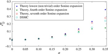
Plot of the second Sonine polynomial expansion coefficient, $h_{{\it\alpha}}^{(2)}$ , for a monodisperse system with Laplace distributed coefficients of restitution around a mean value $\langle e\rangle =0.9$ , as a function of the width of the distribution ${\it\sigma}$ . The theoretical results for different truncation orders of the polynomial expansion (filled circles) are plotted together with DSMC simulation results (empty circles), cf. § 4.

The system of equations (3.26), (3.27), (3.30) for the coefficients $\{h_{A}^{(p)},h_{B}^{(p)},\tilde{{\it\Gamma}}\}$ is to be solved in conjunction with the requirements (3.5)–(3.7) that impose, using (3.25): $h_{A}^{(0)}=1$ , $h_{B}^{(0)}=1$ , $(n_{A}/n)h_{A}^{(1)}+(n_{B}/n)h_{B}^{(1)}=0$ . 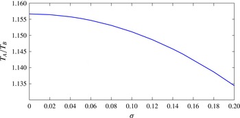Figure 1 shows a comparison between theoretical and (DSMC) simulation values for the coefficient $h_{{\it\alpha}}^{(2)}$ of a monodisperse system obtained within different truncation orders of the polynomial expansion, for Laplace distributed coefficients of restitution (cf. § 4). Employing the expression (3.25) in (2.7) allows one to compute the ratio of temperatures between the two species. Figure 2 shows the dependence of this ratio on the width of the (Laplace) distribution for the coefficients of restitution in the case of a mixture having a mass ratio $m_{A}/m_{B}=4$ . The equations corresponding to the gradient-induced corrections of the distribution functions, (3.9)–(3.13), are solved by proceeding as for the homogeneous inelastic corrections ${\it\phi}_{{\it\alpha}}^{(0)}$ to the Maxwellian distribution. The isotropic functions ${\it\Phi}_{{\it\alpha}}^{K,X}$ , $X\in \{T,c,n,V\}$ are expressed as truncated series of Sonine polynomials:

Figure 2.

The temperature ratio $T_{A}/T_{B}$ for a mixture of particles having the same size and number density and a mass ratio $m_{A}/m_{B}=4$ , with Laplace distributed coefficients of restitution around a mean value $\langle e\rangle =0.9$ , as a function of the width of the distribution ${\it\sigma}$ .

(3.32) $$\begin{eqnarray}\displaystyle & \displaystyle {\it\Phi}_{{\it\alpha}}^{K,T}=\mathop{\sum }_{p=0}^{N_{t}}\frac{k_{{\it\alpha}}^{T,(p)}}{nd_{AB}^{2}}S_{3/2}^{p}({\it\gamma}_{{\it\alpha}}u^{2})=\mathop{\sum }_{p=0}^{N_{t}}\frac{k_{{\it\alpha}}^{T,(p)}}{nd_{AB}^{2}}\widetilde{\partial }_{t^{p}}G_{3/2}(t,{\it\gamma}_{{\it\alpha}}u^{2}) & \displaystyle\end{eqnarray}$$

(3.33) $$\begin{eqnarray}\displaystyle & \displaystyle {\it\Phi}_{{\it\alpha}}^{K,n}=\mathop{\sum }_{p=0}^{N_{t}}\frac{k_{{\it\alpha}}^{n,(p)}}{nd_{AB}^{2}}S_{3/2}^{p}({\it\gamma}_{{\it\alpha}}u^{2})=\mathop{\sum }_{p=0}^{N_{t}}\frac{k_{{\it\alpha}}^{n,(p)}}{nd_{AB}^{2}}\widetilde{\partial }_{t^{p}}G_{3/2}(t,{\it\gamma}_{{\it\alpha}}u^{2}) & \displaystyle\end{eqnarray}$$

(3.34) $$\begin{eqnarray}\displaystyle & \displaystyle {\it\Phi}_{{\it\alpha}}^{K,c}=\mathop{\sum }_{p=0}^{N_{t}}\frac{k_{{\it\alpha}}^{c,(p)}}{nd_{AB}^{2}}S_{3/2}^{p}({\it\gamma}_{{\it\alpha}}u^{2})=\mathop{\sum }_{p=0}^{N_{t}}\frac{k_{{\it\alpha}}^{c,(p)}}{nd_{AB}^{2}}\widetilde{\partial }_{t^{p}}G_{3/2}(t,{\it\gamma}_{{\it\alpha}}u^{2}) & \displaystyle\end{eqnarray}$$

(3.35) $$\begin{eqnarray}\displaystyle & \displaystyle {\it\Phi}_{{\it\alpha}}^{K,V}=\mathop{\sum }_{p=0}^{N_{t}}\frac{k_{{\it\alpha}}^{V,(p)}}{nd_{AB}^{2}}S_{5/2}^{p}({\it\gamma}_{{\it\alpha}}u^{2})=\mathop{\sum }_{p=0}^{N_{t}}\frac{k_{{\it\alpha}}^{V,(p)}}{nd_{AB}^{2}}\widetilde{\partial }_{t^{p}}G_{5/2}(t,{\it\gamma}_{{\it\alpha}}u^{2}), & \displaystyle\end{eqnarray}$$

which are substituted in (3.9)–(3.13). The resulting set of equations is then projected on

(3.36) $$\begin{eqnarray}S_{3/2}^{N}({\it\gamma}_{{\it\alpha}}u^{2})\sqrt{{\it\gamma}_{{\it\alpha}}}\boldsymbol{u}=\tilde{\partial }_{w^{N}}G_{3/2}(w,{\it\gamma}_{{\it\alpha}}u^{2})\sqrt{{\it\gamma}_{{\it\alpha}}}\boldsymbol{u},\end{eqnarray}$$

for $X\in \{T,c,n\}$ , and

(3.37) $$\begin{eqnarray}S_{5/2}^{N}({\it\gamma}_{{\it\alpha}}u^{2}){\it\gamma}_{{\it\alpha}}^{3/2}\overline{\boldsymbol{u}\boldsymbol{u}}=\tilde{\partial }_{w^{N}}G_{5/2}(w,{\it\gamma}_{{\it\alpha}}u^{2}){\it\gamma}_{{\it\alpha}}^{3/2}\overline{\boldsymbol{u}\boldsymbol{u}},\end{eqnarray}$$

for $X=V$ . One then obtains a linear system of equations for the coefficients $k_{{\it\alpha}}^{X,(p)}$ :

(3.38) $$\begin{eqnarray}\unicode[STIX]{x1D648}^{K}\underline{\boldsymbol{k}}=\underline{\boldsymbol{R}}^{K},\end{eqnarray}$$

where $\underline{\boldsymbol{k}}$ is the column vector defined by: $\underline{\boldsymbol{k}}\equiv (k_{A}^{T,(0)},\ldots ,k_{A}^{T,(N)},k_{B}^{T,(0)},\ldots ,k_{B}^{T,(N)},k_{A}^{n,(0)},\ldots ,k_{A}^{n,(N)},k_{B}^{n,(0)},\ldots ,k_{B}^{n,(N)},k_{A}^{c,(0)},\ldots ,k_{A}^{c,(N)},k_{B}^{c,(0)},\ldots ,k_{B}^{c,(N)},k_{A}^{V,(0)},\ldots ,k_{A}^{V,(N)},k_{B}^{V,(0)},\ldots ,k_{B}^{V,(N)})^{\text{t}}$ , the superscript t, standing here for ‘transpose’. The matrix elements, $\unicode[STIX]{x1D614}_{ij}^{K}$ and $\unicode[STIX]{x1D619}_{j}^{K}$ defined in (3.38), and their generating functions, are given in appendix B. In addition, the constraints (3.5)–(3.7), yield, for $X\in \{T,n,c\}$ :

(3.39) $$\begin{eqnarray}\frac{n_{A}}{n}\sqrt{m_{A}}k_{A}^{X,(0)}+\frac{n_{B}}{n}\sqrt{m_{B}}k_{B}^{X,(0)}=0.\end{eqnarray}$$

Using the forms (3.8), (3.32)–(3.35), in conjunction with the solution $\{k_{{\it\alpha}}^{X,(q)}\}$ , where $0\leqslant q\leqslant N_{t}$ , for the system (3.38), in the definitions of the diffusion velocity, heat flux and stress tensor, one obtains the constitutive relations. The resulting transport coefficients (like the coefficients $\{k_{{\it\alpha}}^{X,(q)}\}$ ), are non-trivial functions of the mass and size ratios, concentration and of the characteristics of the distributions ${\it\rho}_{{\it\alpha}{\it\beta}}(e)$ for the coefficient of restitution. Note that the functions ${\it\phi}_{A}^{K}$ and ${\it\phi}_{B}^{K}$ (cf. (3.8)) do not contribute to the cooling rate ${\it\Gamma}$ so that to first order in the gradient considered here, ${\it\Gamma}$ is given by (3.30). The pressure $p$ is given by:

(3.40) $$\begin{eqnarray}p=\frac{nT}{3}.\end{eqnarray}$$

The shear viscosity is given by:

(3.41) $$\begin{eqnarray}{\it\mu}=-\frac{\sqrt{6}}{24}\frac{\sqrt{Tm_{0}}}{d_{AB}^{2}}\left(\frac{n_{A}}{n}\sqrt{M_{A}}k_{A}^{V,(0)}+\frac{n_{B}}{n}\sqrt{M_{B}}k_{B}^{V,(0)}\right).\end{eqnarray}$$

The transport coefficients for the diffusion flux are given by:

(3.42) $$\begin{eqnarray}{\bf\kappa}_{A}^{X}=k_{A}^{X,(0)},\end{eqnarray}$$

and the transport coefficients for the heat flux are:

(3.43) $$\begin{eqnarray}{\it\lambda}^{X}=\frac{n_{A}}{n\sqrt{M_{A}}}(k_{A}^{X,(0)}-k_{A}^{X,(1)})+\frac{n_{B}}{n\sqrt{M_{B}}}(k_{B}^{X,(0)}-k_{B}^{X,(1)}).\end{eqnarray}$$

Note that while the transport coefficients are expressed only in terms of the first two Sonine expansion coefficients, their values, as that of the expansion coefficients, actually depend on the order of truncation of the whole series in Sonine polynomials.

4. Comparison with DSMC simulations

To check the reliability of the calculation of the transport coefficients presented above, we numerically solve the Boltzmann equation by means of the DSMC method (Bird Reference Bird1976), using the particle simulator Dynamo (Bannerman, Sargant & Lue Reference Bannerman, Sargant and Lue2011). For binary mixtures, the velocity distribution is estimated by:

(4.1) $$\begin{eqnarray}f_{{\it\alpha}}(v,t)=\frac{1}{N_{{\it\alpha}}}\mathop{\mathop{\sum }^{N_{{\it\alpha}}}}_{i=1}{\it\delta}(\boldsymbol{v}-\boldsymbol{v}_{(i)}(t)),\end{eqnarray}$$

where $N_{{\it\alpha}}$ is the number of particles in species ${\it\alpha}$ , and the indices in brackets indicate a given particle label.

Considering first the influence of the stochastic behaviour of the coefficient of restitution on the reduced velocity distribution function of a homogeneous monodisperse granular gas, we performed a DSMC simulation of a system with $N\equiv N_{A}+N_{B}=5\times 10^{5}$ particles, recorded the velocities of the particles after $10^{5}$ collisions and evaluated the Sonine polynomial expansion coefficients of the distribution function.

The latter are related to the velocity moments

(4.2) $$\begin{eqnarray}c^{2k}\equiv \frac{1}{N}\mathop{\sum }_{i=1}^{N}\left(\frac{\boldsymbol{v}_{(i)}\boldsymbol{v}_{(i)}}{2T}\right)^{k}\end{eqnarray}$$

through (Chapman & Cowling Reference Chapman and Cowling1970):

(4.3) $$\begin{eqnarray}c^{2k}=\frac{(2k+1)!!}{2^{k}}\left(1+\mathop{\sum }_{p}(-1)^{p}\frac{k!}{(k-p)!p!}h_{{\it\alpha}}^{(p)}\right).\end{eqnarray}$$

Figure 1 shows theoretical predictions for $h_{{\it\alpha}}^{(2)}$ (corresponding to different truncations of the polynomial series) together with DSMC results. Guided by recent experimental, numerical and theoretical results (Montaine et al. Reference Montaine, Heckel, Kruelle, Schwager and Pöschel2011; Gunkelmann et al. Reference Gunkelmann, Montaine and Poschel2014) concerning the distribution of coefficients of restitution, we considered here the case of Laplace distributed coefficients:

(4.4) $$\begin{eqnarray}{\it\rho}_{{\it\alpha}{\it\beta}}(e)=\frac{1}{2{\it\sigma}_{{\it\alpha}{\it\beta}}}\text{e}^{(-|e-\langle e\rangle _{{\it\alpha}{\it\beta}}|)/{\it\sigma}_{{\it\alpha}{\it\beta}}}.\end{eqnarray}$$

In our simulation, at each time step, $N_{p}^{{\it\alpha}{\it\beta}}$ pairs of (simulated) particles are selected randomly with equal probability, where $N_{p}^{{\it\alpha}{\it\beta}}$ corresponds to the maximum of the probable number of collisions occurring along the direction spanned by $\boldsymbol{k}$ between a given particle of species ${\it\alpha}$ travelling with velocity $\boldsymbol{v}_{1}$ and a particle of species ${\it\beta}$ with velocity $\boldsymbol{v}_{2}$ during a time interval ${\rm\Delta}t_{{\it\alpha}{\it\beta}}$ , and reads (in the dilute case considered here):

(4.5) $$\begin{eqnarray}N_{p}^{{\it\alpha}{\it\beta}}=2N_{{\it\alpha}}{\rm\pi}n_{{\it\beta}}\max [d_{{\it\alpha}{\it\beta}}^{2}(\boldsymbol{v}_{12}\boldsymbol{\cdot }\boldsymbol{k}){\bf\theta}(\boldsymbol{v}_{12}\boldsymbol{\cdot }\boldsymbol{k})]{\rm\Delta}t_{{\it\alpha}{\it\beta}},\end{eqnarray}$$

where ${\it\theta}$ is the Heaviside step function, and ${\rm\Delta}t_{{\it\alpha}{\it\beta}}$ describes the rate at which particles of species ${\it\alpha}$ are tested for collisions. A collision is executed with a probability $w_{{\it\alpha}{\it\beta}}$ given by:

(4.6) $$\begin{eqnarray}w_{{\it\alpha}{\it\beta}}=\frac{d_{{\it\alpha}{\it\beta}}^{2}(\boldsymbol{v}_{12}\boldsymbol{\cdot }\boldsymbol{k}){\bf\theta}(\boldsymbol{v}_{12}\boldsymbol{\cdot }\boldsymbol{k})}{\max [d_{{\it\alpha}{\it\beta}}^{2}(\boldsymbol{v}_{12}\boldsymbol{\cdot }\boldsymbol{k}){\bf\theta}(\boldsymbol{v}_{12}\boldsymbol{\cdot }\boldsymbol{k})]}.\end{eqnarray}$$

When a collision occurs, the velocities are updated according to the collision rule, (2.1), where the coefficient of restitution is drawn from the probability distribution, (4.4). The average value of the coefficient of restitution was taken to be $\langle e\rangle \equiv \langle e\rangle _{AA}=\langle e\rangle _{AB}=\langle e\rangle _{BB}=0.9$ , and we varied the width ${\it\sigma}\equiv {\it\sigma}_{AA}={\it\sigma}_{AB}={\it\sigma}_{BB}$ of its probability density. For the smaller standard deviations ${\it\sigma}$ , DSMC and theory are in fairly good agreement, while as ${\it\sigma}$ increases, discrepancies between simulation and theoretical predictions become larger, illustrating the need for high-order truncation in the polynomial expansions. Notice that for large values of ${\it\sigma}$ , the coefficient of restitution can take positive values with non-zero probability, traducing the fact that, in the context of the experiments and simulations which inspired the form of the distributions ${\it\rho}_{{\it\alpha}{\it\beta}}$ , the fluctuating nature of the coefficient of restitution finds its origin in the exchange of energy between translational and rotational degrees of freedom, so that translational energy can occasionaly increase in a given collision (the rate of decay ${\it\Gamma}$ must however always be positive). We considered next the diffusion of impurities, described by the tracer limit ( $c\rightarrow 0$ ) of the diffusion coefficient ${\it\kappa}_{A}^{c}$ .

Figure 3.

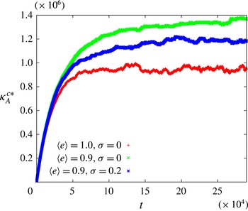
Plot of the reduced mutual diffusion coefficient as a function of time, in units of accumulated number of collisions, for different parameters of the Laplace distributed coefficient of restitution.

In this limit, the coefficient can be measured from the mean-square displacement of the tracer particles in the homogeneous cooling state:

(4.7) $$\begin{eqnarray}{\it\kappa}_{A}^{c}(t)=\frac{n_{B}}{6{\it\delta}t}\frac{1}{N_{B}}\mathop{\sum }_{i=1}^{N_{B}}[|\boldsymbol{r}_{(i)}(t+{\it\delta}t)-\boldsymbol{r}_{(i)}(0)|^{2}-|\boldsymbol{r}_{(i)}(t)-\boldsymbol{r}_{(i)}(0)|^{2}],\end{eqnarray}$$

where ${\it\delta}t$ denotes a time interval, $n_{B}$ is the number density of the gas in excess and the above sum is carried out over $B$ particles. The tracer limit (of species $A$ ) is realized in the simulations by ignoring $A$ – $A$ collisions, and by imposing that the tracer particles have no influence on the dynamics of the surrounding gas, i.e. in $A$ – $B$ collisions, only the velocity of $A$ (tracer) particles are modified (notice that exceptions to the validity of this last part of the procedure for reproducing the tracer limit have been reported in the case of the ‘vanilla plain’ Maxwell model of interparticles interaction (Garzo & Trizac Reference Garzo and Trizac2011), but outside the range parameters considered here). A small number of particles $A$ is therefore not required (Garzo & Montanero Reference Garzo and Montanero2004). In order to get rid of the time dependence of the diffusion coefficient that occurs through its dependence on the (decreasing in time) temperature, we consider a reduced diffusion coefficient ${\it\kappa}_{A}^{c\ast }$ :

(4.8) $$\begin{eqnarray}{\it\kappa}_{A}^{c\ast }(t)=\frac{{\it\kappa}_{A}^{c}(t)}{\sqrt{T(t)}}.\end{eqnarray}$$

The above rescaling allows us to eliminate the time dependence of ${\it\kappa}_{A}^{c\ast }$ , as can be seen in figure 3. The latter shows the time behaviour of ${\it\kappa}_{A}^{c\ast }$ obtained in a simulation of a mixture of 13 500 particles (half of which belonging to the impurity species $A$ ), having identical sizes and mass ratio $m_{A}/m_{B}=4$ , performing $10^{5}$ collisions, with coefficients of restitution distributed according to Laplace laws (4.4) with identical averages and variances $\langle e\rangle =\langle e\rangle _{AA}=\langle e\rangle _{AB}=\langle e\rangle _{BB}$ , and ${\it\sigma}={\it\sigma}_{AA}={\it\sigma}_{AB}={\it\sigma}_{BB}$ . 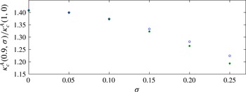After a transient regime, the value of the coefficient ${\it\kappa}_{A}^{c\ast }$ reaches a constant value. A comparison of the corresponding value of the diffusion coefficient, normalized by its elastic counterpart, with theoretical predictions for $\langle e\rangle =0.9$ and various values of ${\it\sigma}$ is shown in figure 4.

Figure 4.

Comparison between theoretical (empty circles) and DSMC results (filled circles) for the normalized diffusion coefficient ${\it\kappa}_{c}^{A}(\langle e\rangle ,{\it\sigma})/{\it\kappa}_{c}^{A}(1,0)$ computed in the tracer limit $n_{A}/n\rightarrow 0$ , for a mass ratio $m_{A}/m_{B}=4$ , and a restitution coefficient distributed according to a Laplace law around $\langle e\rangle =0.9$ . The values are plotted as a function of the width ${\it\sigma}$ of the Laplace distribution for the coefficients of restitution.

5. Stochasticity-induced segregation

As has been illustrated in the previous section, taking into account the stochastic nature of the coefficient of restitution can have a quantitative influence on the values of the transport coefficient. The importance of this effect depends of course on the actual shape of the distribution, and in particular its width. This section is devoted to the study of a qualitative signature of the stochasticity, namely, the fact that the shape of the distribution influences segregation in mixtures of otherwise identical particles. More specifically, we study temperature and gravity driven diffusion in a mixture of grains with the same mass, size and mean coefficient of restitution, but different standard deviations for the (three) different types of restitution coefficient. Thermal segregation in granular mixtures has been identified as one of the main factors of the Brazil Nut effect (Hsiau & Hunt Reference Hsiau and Hunt1996; Schröter et al. Reference Schröter, Ulrich, Kreft, Swift and Swinney2006) in the case of granular gases, and its dependence on the particle properties has been studied in the past (Arnarson & Willits Reference Arnarson and Willits1998; Jenkins & Yoon Reference Jenkins and Yoon2002; Brey et al. Reference Brey, Ruiz-Montero and Moreno2005; Garzó Reference Garzó2008). In particular, it was predicted (Serero et al. Reference Serero, Goldhirsch, Noskowicz and Tan2006) and observed in molecular dynamic simulations (Brito et al. Reference Brito, Enriquez, Godoy and Soto2008; Brito & Soto Reference Brito and Soto2009; Serero et al. Reference Serero, Noskowicz, Tan and Goldhirsch2009; Serero, Noskowicz & Goldhirsch Reference Serero, Noskowicz and Goldhirsch2011) that the species in a binary mixture may segregate even when they differ only in their respective coefficients of restitution, demonstrating a direct influence of inelasticity on the properties of binary granular gas mixtures. Here, we proceed with a similar analysis by considering particles of the same mass, size and average coefficient of restitution, and Laplacian distributions for the three types of coefficient of restitution, with different standard deviations. The momentum balance equation describing the non-convecting ( $\boldsymbol{V}=0$ ) steady state of a mixture reads, using (2.11) (after adding ${\it\rho}_{m}\boldsymbol{g}$ on the left-hand side, to account for gravity), and (3.20):

(5.1) $$\begin{eqnarray}\boldsymbol{{\rm\nabla}}p=-{\it\rho}_{m}\boldsymbol{g},\end{eqnarray}$$

which can be rewritten using the equation of state $p=nT/3$ :

(5.2) $$\begin{eqnarray}\boldsymbol{{\rm\nabla}}\ln n=-\boldsymbol{{\rm\nabla}}\ln T-\frac{3}{T}((m_{A}-m_{B})c+m_{B})\boldsymbol{g}.\end{eqnarray}$$

Figure 5.

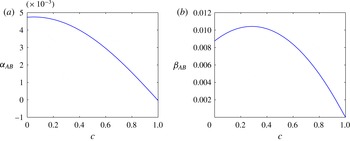
Plots of the thermal coefficients ${\it\alpha}_{AB}$ and ${\it\beta}_{AB}$ , see (5.4)–(5.5), as a function of the concentration, $c\equiv n_{A}/n$ , for a mixture of particles whose collisions are characterized by coefficients of restitution distributed according to Laplace laws. The distributions have the same average coefficients of restitution $\langle e\rangle =\sqrt{0.8}$ , and different standard deviations for the three type of collisions: ${\it\sigma}_{AA}=0.2$ , ${\it\sigma}_{AB}=0.1$ , and ${\it\sigma}_{BB}=0.01$ . The particles are otherwise identical, i.e.  $m_{A}=m_{B}$ , $d_{A}=d_{B}$ .

Now substituting (5.2) in (3.16), and using the fact that the diffusive fluxes vanish ( $\boldsymbol{J}_{A}=0$ ), one obtains the following relation between the temperature and concentration gradients, when the temperature and concentration vary only along the vertical ( $z$ ) direction:

(5.3) $$\begin{eqnarray}\frac{\partial \ln c}{\partial {\it\xi}}={\it\alpha}_{AB}\frac{\partial \ln T}{\partial {\it\xi}}+{\it\beta}_{AB},\end{eqnarray}$$

where ${\it\xi}=\int _{0}^{z}(((m_{A}+m_{B})g)/T(z^{\prime }))\,\text{d}z^{\prime }$ , is a rescaled length scale,

(5.4) $$\begin{eqnarray}{\it\alpha}_{AB}\equiv \frac{{\it\kappa}_{A}^{n}-{\it\kappa}_{A}^{T}}{{\it\kappa}_{A}^{c}},\end{eqnarray}$$

describes the effects of the temperature gradient on the gradient of concentration, and

(5.5) $$\begin{eqnarray}{\it\beta}_{AB}=3\frac{{\it\kappa}_{A}^{n}}{{\it\kappa}_{A}^{c}}((M_{A}-M_{B})c+M_{B}),\end{eqnarray}$$

accounts for the effects of gravity. In particular, the sign of ${\it\alpha}_{AB}$ determines the direction of segregation: when ${\it\alpha}_{AB}>0$ the $A$ particles tend to concentrate in the hotter regions. Similarly, when ${\it\beta}_{AB}>0$ the particles $A$ tend to concentrate near the top of the system. As mentioned, in order to emphasize the effect of the random nature of the coefficient of restitution on the segregation properties of the system, we consider here the case $m_{A}=m_{B}$ , $d_{A}=d_{B}$ , and $\langle e\rangle _{AA}=\langle e\rangle _{AB}=\langle e\rangle _{BB}=\sqrt{0.8}$ , i.e. we study a mixture of particles differing only in the shape of the distribution of the coefficient of restitution characterizing the collisions they are subjected to. More specifically, we consider a set of Laplacian distributions, with three different widths ${\it\sigma}_{AA}=0.2$ , ${\it\sigma}_{AB}=0.1$ and ${\it\sigma}_{BB}=0.01$ . The corresponding values for the coefficients ${\it\alpha}_{AB}$ and ${\it\beta}_{AB}$ are plotted in figure 5 as functions of the concentration, $c$ , of $A$ particles. The sign of ${\it\alpha}_{AB}$ indicates that the particles with the broader distribution tend to concentrate in the hotter regions. The sign of ${\it\beta}_{AB}$ (figure 5 b) indicates that gravity drives the particles with broader distribution upward. Associated with the fact that in a vertically vibrated system of such mixtures, a minimum in the temperature profile is expected (Brey, Ruiz-Montero & Moreno Reference Brey, Ruiz-Montero and Moreno2001; Brey & Ruiz-Montero Reference Brey and Ruiz-Montero2004), as a consequence of the density gradient correction to the Fourier law, these results may suggest the possibility of a pattern formation in the form of a three layer arrangement in vertically vibrated systems, similar to those predicted in Serero et al. (Reference Serero, Goldhirsch, Noskowicz and Tan2006), with the particles colliding with the narrower distribution concentrating in the area situated below the minimum of temperature, as a result of the competition between the effect of the temperature gradient and gravity. For other sets of values of the widths of the distributions, or other types of distributions, one may find that the signs of the coefficients ${\it\alpha}_{AB}$ and ${\it\beta}_{AB}$ depend on the concentration, yielding more complex interplay between the effects of gravity and of the temperature gradients, and suggesting the possibility of different profiles of concentration.

6. Concluding remarks

A complete hydrodynamic description of a dilute binary mixture of granular gas interacting by collisions characterized by stochastic coefficients of restitution has been derived. A technique for obtaining accurate transport coefficients, limited only by computer capacity, has also been presented. The method has been illustrated by considering the case of Laplacian distributions, which can be used to model energy transfer to integral degrees of freedom due to surface asperities, as has been recently shown in experiments and simulations. The results were compared to DSMC simulations with good agreement. The stochasticity has been shown to yield quantitative differences with respect to the non-fluctuating case. Of course the discrepancies depend strongly on the actual shape of the employed distribution function; typically, wider distributions yield stronger discrepancies. The hydrodynamic description has been employed to study the segregation in a mixture subjected to a temperature gradient under gravity. In particular, by considering a mixture of two species having the same mass and size, and interacting with the same coefficient of restitution on average, it was shown that fluctuation of the coefficient of restitution alone was sufficient to yield partial segregation. Particles whose collisions are characterized by wider distributions for the coefficient of restitution were found to tend to be driven towards the hotter regions, while gravity was found to drive those particles upward. While we considered as an illustration a particular type of distribution, the hydrodynamic description presented here, and the described method for obtaining the transport coefficients could be applied to the effective description of the relevant degrees of freedom of other dissipative collisional systems, provided a probability distribution for the exchange of energy with the remaining degrees of freedom can be devised. Those possibly comprise, e.g. complex shaped particles or some classes of active particles.