2.1. Left-truncated and right-censored data

In many survival analysis applications, observed lifetime data are often subject to LTRC. Left truncation occurs when a subject is included in a study only if they have survived beyond a certain threshold, meaning that subjects who fail before the threshold are excluded from the dataset. Right censoring arises when the observation period terminates before the failure event occurs; in such cases, the exact failure time is unknown but is known to exceed the censoring time.

The observed data consist of a set of triplets, denoted by

\begin{align*} \mathcal{D} = \{(t_1, \tau_1, \delta_1), \ldots, (t_n, \tau_n, \delta_n)\}, \end{align*}

where $t_i$ represents either the observed failure time or the right-censoring time for the ith subject, and $\tau_i$ denotes the left-truncation time. If $\tau_i = 0$ then no left truncation occurs for that subject. The indicator variable $\delta_i$ denotes right censoring, with $\delta_i = 1$ indicating that $t_i$ is a failure time and $\delta_i = 0$ indicating that the failure time exceeds $t_i$ but is not observed.

Now, consider the likelihood function for the LTRC data under a given failure-time distribution. Assume that the failure times of all subjects are i.i.d. random variables denoted by T. Let $S(t;\, \boldsymbol{\theta})$ and $f(t;\, \boldsymbol{\theta})$ be the survival and probability density functions (p.d.f.s) of the failure-time distribution, respectively, where $\boldsymbol{\theta}$ is the parameter vector to be estimated. These are defined by

\begin{align*} S(t;\, \boldsymbol{\theta}) = \textrm{P}(T > t), \quad f(t;\, \boldsymbol{\theta}) = -\frac{\mathrm{d}}{\mathrm{d} t} S(t;\, \boldsymbol{\theta}). \end{align*}

Due to left truncation, the likelihood must condition on each observation $T_i > \tau_i$ . This leads to a likelihood formulation using the conditional survival function $S(t \mid T > \tau;\, \boldsymbol{\theta})$ and conditional density $f(t \mid T > \tau;\, \boldsymbol{\theta})$ . The log-likelihood function (LLF) for the observed data $\mathcal{D}$ is given by

\begin{align*} \mathcal{L}(\boldsymbol{\theta};\ \mathcal{D}) = \sum_{i=1}^n \left[ \delta_i \log f(t_i \mid T > \tau_i;\, \boldsymbol{\theta}) + (1 - \delta_i) \log S(t_i \mid T > \tau_i;\ \boldsymbol{\theta}) \right]. \end{align*}

The maximum-likelihood (ML) estimator is obtained by maximizing $\mathcal{L}(\boldsymbol{\theta};\, \mathcal{D})$ with respect to  $\boldsymbol{\theta}$ .

2.2. PH distribution

A continuous PH distribution is defined as the distribution of the time to absorption in a CTMC. Let $\{X_t \,:\, t \ge 0\}$ denote a CTMC with m transient states (phases) and a single absorbing state. The PH-distributed random variable T represents the time until the process $X_t$ enters the absorbing state.

Let $\boldsymbol{\alpha} = (\alpha_1, \ldots, \alpha_m)$ denote the initial probability vector over the transient states, and let $\boldsymbol{T}$ denote the $m \times m$ infinitesimal generator matrix over the transient states. The cumulative distribution function (c.d.f.) and p.d.f. of the PH distribution are given by

\begin{align*} F_{\mathrm{PH}}(t) = 1 - \boldsymbol{\alpha} \exp(\boldsymbol{T} t) \boldsymbol{1}, \quad f_{\mathrm{PH}}(t) = \boldsymbol{\alpha} \exp(\boldsymbol{T} t) \boldsymbol{\xi}, \end{align*}

where $\boldsymbol{1}$ is a column vector of ones, and $\boldsymbol{\xi} = ( \xi_1, \ldots, \xi_m )^\top$ is the exit-rate vector, with $\xi_i$ denoting the transition rate from phase i to the absorbing state. Let $\lambda_{i,j}$ (for $i \neq j$ ) be the (i, j)th entry of $\boldsymbol{T}$ , representing the transition rate from phase i to phase j. The total exit rate from phase i is defined as $\lambda_i = \sum_{j \neq i} \lambda_{i,j} + \xi_i$ . Hence, the diagonal entries of $\boldsymbol{T}$ are given by $-\lambda_i$ , that is, $\boldsymbol{T}$ has negative diagonal entries. Consequently, it follows that $\boldsymbol{\xi} = -\boldsymbol{T} \boldsymbol{1}$ .

In general, a PH distribution can be parameterized by the pair $(\boldsymbol{\alpha}, \boldsymbol{T})$ . However, in this study, we treat $\boldsymbol{\xi}$ as an explicit parameter for the sake of notational clarity and computational efficiency. The objective is to estimate the parameters $\boldsymbol{\alpha}$ , $\boldsymbol{T}$ , and $\boldsymbol{\xi}$ from the LTRC data.

3.1. General PH case

The EM algorithm is an iterative procedure for computing ML estimates with incomplete data [Reference Dempster, Laird and Rubin10, Reference Wu21]. Let $\mathcal{D}$ and $\mathcal{U}$ be the observed and unobserved data vectors, respectively. The goal is to estimate the model parameter vector $\boldsymbol{\theta}$ from the observed data $\mathcal{D}$ within the EM framework, which treats the unobserved variables as latent data. The EM algorithm consists of two steps: the expectation step (E-step) and the maximization step (M-step). In the E-step, the conditional expectation of the complete-data LLF is computed given the observed data. The M-step updates the parameters by maximizing this conditional expected LLF.

Suppose that $\mathcal{D}$ is the LTRC dataset. To apply the EM algorithm, we must define the unobserved data $\mathcal{U}$ . Let $U^{(k)}$ denote the number of unobserved subjects corresponding to the kth observation due to left truncation. That is, when left truncation occurs, several subjects may experience failure before truncation time $\tau_k$ ; these unobserved failures are treated as latent data. Furthermore, let $T^{(k,l)}$ , for $l = 1, \ldots, U^{(k)}$ , denote the failure time of the lth subject whose lifetime terminates before the left-truncation time $\tau_k$ . For notational convenience, $T^{(k,l)}$ with $l = U^{(k)}+1$ is defined as the failure time corresponding to the kth observation that is not truncated.

In addition, we define the following unobserved random variables related to the phase transitions. Let $B_i^{(k,l)}$ be an indicator random variable for the event that the phase process associated with $T^{(k,l)}$ begins in phase i. Let $Z_i^{(k,l)}$ denote the total sojourn time spent in phase i by the phase process of $T^{(k,l)}$ . Let $Y_i^{(k,l)}$ be an indicator random variable for the event that the phase process of $T^{(k,l)}$ visits phase i just before absorption. Finally, let $N_{i,j}^{(k,l)}$ denote the total number of transitions from phase i to phase j in the phase process of $T^{(k,l)}$ .

Based on the above definitions, the set of unobserved random variables is given by

\begin{align*} \mathcal{U}=\left\{U^{(k)}, B_i^{(k,l)}, Z_i^{(k,l)}, Y_i^{(k,l)}, N_{i,j}^{(k,l)}\right\} \quad\text{for all } k, l. \end{align*}

The complete-data likelihood function is then expressed as

\begin{align*} p(\mathcal{D}, \mathcal{U};\ \boldsymbol{\theta}) = \prod_{k=1}^{n} \prod_{l=1}^{U^{(k)}+1} \left( \prod_{i=1}^m \alpha_i^{B_i^{(k,l)}} \prod_{i=1}^m \exp\left(-\lambda_{i} Z_i^{(k,l)} \right) \prod_{i=1}^m \prod_{{j=1}, \, {j\not=i}}^m \lambda_{i,j}^{N_{i,j}^{(k,l)}} \prod_{i=1}^m \xi_i^{Y_i^{(k,l)}} \right), \end{align*}

where $p(\! \cdot \!)$ denotes the appropriate density or mass function. Assuming that the observed data $(t_k, \tau_k, \delta_k)$ are mutually independent for $k=1, \ldots, n$ , the following M-step updates are obtained by maximizing the expected complete-data LLF

\begin{align*}&\alpha_i \, :\!= \, \frac{\sum_{k=1}^n \mathrm{E} \Big[ \sum_{l=1}^{U^{(k)}+1} B_i^{(k,l)} \mid \mathcal{D}_k;\, \boldsymbol{\theta} \Big]}{n + \sum_{k=1}^n \mathrm{E}\big[U^{(k)} \mid \mathcal{D}_k;\, \boldsymbol{\theta}\big]}, \quad i = 1, \ldots, m, \\[3pt]&\xi_i \, :\!= \, \frac{\sum_{k=1}^n \mathrm{E}\Big[ \sum_{l=1}^{U^{(k)}+1} Y_i^{(k,l)} \mid \mathcal{D}_k;\, \boldsymbol{\theta} \Big]}{\sum_{k=1}^n \mathrm{E}\Big[ \sum_{l=1}^{U^{(k)}+1} Z_i^{(k,l)} \mid \mathcal{D}_k;\, \boldsymbol{\theta} \Big]}, \quad i = 1, \ldots, m, \\[3pt]&\lambda_{i,j} \, :\!= \, \frac{\sum_{k=1}^n \mathrm{E}\Big[ \sum_{l=1}^{U^{(k)}+1} N_{i,j}^{(k,l)} \mid \mathcal{D}_k;\, \boldsymbol{\theta} \Big]}{\sum_{k=1}^n \mathrm{E}\Big[ \sum_{l=1}^{U^{(k)}+1} Z_i^{(k,l)} \mid \mathcal{D}_k;\, \boldsymbol{\theta} \Big]}, \quad i = 1, \ldots, m, \ j = 1, \ldots, m, \ i \not=j,\end{align*}

where $\mathcal{D}_k = (t_k, \tau_k, \delta_k)$ .

Next, we derive the E-step formulas. By marginalizing the complete-data likelihood function with respect to $U^{(k)}$ , we obtain

\begin{align*} p(U^{(k)} | \mathcal{D}_k;\, \boldsymbol{\theta}) \propto \left(\int_0^{\tau_k} f_{\mathrm{PH}}(t;\, \boldsymbol{\theta}) \,\mathrm{d} t \right)^{U^{(k)}}, \quad U^{(k)} = 0, 1, 2, \ldots. \end{align*}

This indicates that the posterior distribution of $U^{(k)}$ follows a geometric distribution with failure probability $\int_0^{\tau_k} f_{\mathrm{PH}}(t;\, \boldsymbol{\theta}) \,\mathrm{d} t$ . Accordingly, the expected value of $U^{(k)}$ is given by

\begin{align*} \mathrm{E}[U^{(k)} \mid \mathcal{D}_k;\, \boldsymbol{\theta}] = \frac{\int_0^{\tau_k} f_{\mathrm{PH}}(t;\, \boldsymbol{\theta}) \,\mathrm{d} t }{1 - \int_0^{\tau_k} f_{\mathrm{PH}}(t;\, \boldsymbol{\theta}) \,\mathrm{d} t} = \frac{1 - \boldsymbol{\alpha} \exp(\boldsymbol{T} \tau_k) \boldsymbol{1}}{\boldsymbol{\alpha} \exp(\boldsymbol{T} \tau_k) \boldsymbol{1}}. \end{align*}

Let $\mathcal{X}_{[0,T]} \, :\!= \, \{X_s \,:\, 0 \le s \le T\}$ denote the path of the phase process associated with T up to its absorption, and let $h(\mathcal{X}_{[0,T]})$ be a measurable functional of this path. Then, we can derive the following expression for the expected value of $U^{(k)}$ and $h(\mathcal{X}_{[0,T^{(k,l)}]})$ :

(1) \begin{align} &\mathrm{E}\left[\left.\sum_{l=1}^{U^{(k)}+1} h(\mathcal{X}_{[0,T^{(k,l)}]}) \right| \mathcal{D}_k;\, \boldsymbol{\theta}\right] = \frac{\int_0^{\tau_k} \mathrm{E}[h(\mathcal{X}_{[0,T]}) \mid T = t;\, \boldsymbol{\theta}]\, f_{\mathrm{PH}}(t;\, \boldsymbol{\theta}) \,\mathrm{d} t}{\boldsymbol{\alpha} \exp(\boldsymbol{T} \tau_k) \boldsymbol{1}} \nonumber\\[4pt] & \qquad + \delta_k \mathrm{E}[h(\mathcal{X}_{[0,T]}) \mid T = t_k;\, \boldsymbol{\theta}] + (1-\delta_k) \mathrm{E}[h(\mathcal{X}_{[0,T]}) \mid T > t_k;\, \boldsymbol{\theta}]. \end{align}

The proof is provided in Appendix A.

By applying (1) to the expected values of $B_i^{(k,l)}$ , $Y_i^{(k,l)}$ , $Z_i^{(k,l)}$ , and $N_{i,j}^{(k,l)}$ , we obtain the following expressions:

\begin{align*} \mathrm{E}\left[ \sum_{l=1}^{U^{(k)}+1} B_i^{(k,l)} \Bigg| \mathcal{D}_k;\, \boldsymbol{\theta} \right] =&\, \frac{\int_0^{\tau_k} \alpha_i [\exp(\boldsymbol{T} t)\boldsymbol{\xi}]_i \,\mathrm{d} t}{\boldsymbol{\alpha} \exp(\boldsymbol{T} \tau_k) \boldsymbol{1}} + \delta_k \frac{\alpha_i [\exp(\boldsymbol{T} t_k) \boldsymbol{\xi}]_i}{\boldsymbol{\alpha} \exp(\boldsymbol{T} t_k) \boldsymbol{\xi}} \\[4pt] & + (1-\delta_k) \frac{\int_{t_k}^\infty \alpha_i [\exp(\boldsymbol{T} t) \boldsymbol{\xi}]_i dt}{\boldsymbol{\alpha} \exp(\boldsymbol{T} t_k) \boldsymbol{1}}, \\[4pt] \mathrm{E}\left[ \sum_{l=1}^{U^{(k)}+1} Y_i^{(k,l)} \Bigg| \mathcal{D}_k;\, \boldsymbol{\theta} \right] =&\, \frac{\int_0^{\tau_k} [\boldsymbol{\alpha} \exp(\boldsymbol{T} t)]_i \xi_i \,\mathrm{d} t}{\boldsymbol{\alpha} \exp(\boldsymbol{T} \tau_k) \boldsymbol{1}} + \delta_k \frac{[\boldsymbol{\alpha} \exp(\boldsymbol{T} t_k)]_i \xi_i}{\boldsymbol{\alpha} \exp(\boldsymbol{T} t_k) \boldsymbol{\xi}} \\[4pt] & + (1-\delta_k) \frac{\int_{t_k}^\infty [\boldsymbol{\alpha} \exp(\boldsymbol{T} t)]_i \xi_i \,\mathrm{d} t}{\boldsymbol{\alpha} \exp(\boldsymbol{T} t_k) \boldsymbol{1}}, \\[4pt] \mathrm{E}\left[ \sum_{l=1}^{U^{(k)}+1} Z_i^{(k,l)} \Bigg| \mathcal{D}_k;\, \boldsymbol{\theta} \right] =&\, \frac{\int_0^{\tau_k} \int_0^{t} [\boldsymbol{\alpha} \exp(\boldsymbol{T} u)]_i [\exp(\boldsymbol{T} (t-u)) \boldsymbol{\xi}]_i \,\mathrm{d} u \,\mathrm{d} t}{\boldsymbol{\alpha} \exp(\boldsymbol{T} \tau_k) \boldsymbol{1}} \\[4pt] & + \delta_k \frac{\int_0^{t_k} [\boldsymbol{\alpha} \exp(\boldsymbol{T} u)]_i [\exp(\boldsymbol{T} (t-u)) \boldsymbol{\xi}]_i \,\mathrm{d} u}{\boldsymbol{\alpha} \exp(\boldsymbol{T} t_k) \boldsymbol{\xi}} \\[4pt] & + (1-\delta_k) \frac{\int_{t_k}^\infty \int_0^{t} [\boldsymbol{\alpha} \exp(\boldsymbol{T} u)]_i [\exp(\boldsymbol{T} (t-u)) \boldsymbol{\xi}]_i \,\mathrm{d} u\,\mathrm{d} t}{\boldsymbol{\alpha} \exp(\boldsymbol{T} t_k) \boldsymbol{1}}, \\[4pt] \mathrm{E}\left[ \sum_{l=1}^{U^{(k)}+1} N_{i,j}^{(k,l)} \Bigg| \mathcal{D}_k;\, \boldsymbol{\theta} \right] =&\, \frac{\int_0^{\tau_k} \int_0^{t} [\boldsymbol{\alpha} \exp(\boldsymbol{T} u)]_i \lambda_{i,j} [\exp(\boldsymbol{T} (t-u)) \boldsymbol{\xi}]_j \,\mathrm{d} u \,\mathrm{d} t}{\boldsymbol{\alpha} \exp(\boldsymbol{T} \tau_k) \boldsymbol{1}} \end{align*}

\begin{align*} & + \delta_k \frac{\int_0^{t} [\boldsymbol{\alpha} \exp(\boldsymbol{T} u)]_i \lambda_{i,j} [\exp(\boldsymbol{T} (t-u)) \boldsymbol{\xi}]_j \,\mathrm{d} u}{\boldsymbol{\alpha} \exp(\boldsymbol{T} t_k) \boldsymbol{\xi}} \\[3pt] & + (1-\delta_k) \frac{\int_{t_k}^\infty \int_0^{t} [\boldsymbol{\alpha} \exp(\boldsymbol{T} u)]_i \lambda_{i,j} [\exp(\boldsymbol{T} (t-u)) \boldsymbol{\xi}]_j \,\mathrm{d} u\,\mathrm{d} t}{\boldsymbol{\alpha} \exp(\boldsymbol{T} t_k) \boldsymbol{1}},\end{align*}

where $[{\cdot}]_i$ is the ith element of the vector.

To facilitate the computation of the above expectations, we introduce the following vectors and matrices:

\begin{align*}&\boldsymbol{f}(t) = \boldsymbol{\alpha} \exp(\boldsymbol{T} t), \quad \overline{\boldsymbol{f}}(t) = \boldsymbol{\alpha} ({-}\boldsymbol{T})^{-1} \exp(\boldsymbol{T} t),\quad \boldsymbol{b}(t) = \exp(\boldsymbol{T} t) \boldsymbol{\xi}, \quad \overline{\boldsymbol{b}}(t) = \exp(\boldsymbol{T} t) \boldsymbol{1}, \\[3pt]& \boldsymbol{H}(t) = \int_0^t \boldsymbol{b}(u) \,\boldsymbol{f}(t-u) \,\mathrm{d} u,\quad \overline{\boldsymbol{H}}(t) = \int_0^t \overline{\boldsymbol{b}}(u) \,\boldsymbol{f}(t-u) \,\mathrm{d} u.\end{align*}

These quantities satisfy the following relationships:

\begin{align*} &\int_t^\infty \int_0^s \boldsymbol{b}(u) \,\boldsymbol{f}(s - u) \,\mathrm{d} u \,\mathrm{d} s = \overline{\boldsymbol{H}}(t) + \boldsymbol{1}\, \overline{\boldsymbol{f}}(t), \\[3pt] &\int_0^t \int_0^s \boldsymbol{b}(u) \,\boldsymbol{f}(s - u) \,\mathrm{d} u \,\mathrm{d} s = \boldsymbol{1} \boldsymbol{\alpha} ({-}\boldsymbol{T})^{-1} - \overline{\boldsymbol{H}}(t) - \boldsymbol{1}\, \overline{\boldsymbol{f}}(t).\end{align*}

Then, the expected values can be expressed as follows:

\begin{align*}\mathrm{E}\left[ \sum_{l=1}^{U^{(k)}+1} B_i^{(k,l)} \Bigg| \mathcal{D}_k;\, \boldsymbol{\theta} \right] =&\, \frac{\alpha_i [\overline{\boldsymbol{b}}(0) - \overline{\boldsymbol{b}}(\tau_k)]_i}{\boldsymbol{\alpha} \overline{\boldsymbol{b}}(\tau_k)}+ \delta_k \frac{\alpha_i [\boldsymbol{b}(t_k)]_i}{\boldsymbol{\alpha} \boldsymbol{b}(t_k)} + (1-\delta_k) \frac{\alpha_i [\overline{\boldsymbol{b}}(t_k)]_i}{\boldsymbol{\alpha} \overline{\boldsymbol{b}}(t_k)}, \\[4pt]\mathrm{E}\left[ \sum_{l=1}^{U^{(k)}+1} Y_i^{(k,l)} \Bigg| \mathcal{D}_k;\, \boldsymbol{\theta} \right] =&\, \frac{[\overline{\boldsymbol{f}}(0) - \overline{\boldsymbol{f}}(\tau_k)]_i \xi_i}{\boldsymbol{\alpha} \overline{\boldsymbol{b}}(\tau_k)}+ \delta_k \frac{[\boldsymbol{f}(t_k)]_i \xi_i}{\boldsymbol{\alpha} \boldsymbol{b}(t_k)} + (1-\delta_k) \frac{[\overline{\boldsymbol{f}}(t_k)]_i \xi_i}{\boldsymbol{\alpha} \overline{\boldsymbol{b}}(t_k)}, \\[4pt]\mathrm{E}\left[ \sum_{l=1}^{U^{(k)}+1} Z_i^{(k,l)} \Bigg| \mathcal{D}_k;\, \boldsymbol{\theta} \right] =&\, \frac{[\overline{\boldsymbol{b}}(0)\, \overline{\boldsymbol{f}}(0) - \overline{\boldsymbol{b}}(0)\, \overline{\boldsymbol{f}}(\tau_k) - \overline{\boldsymbol{H}}(\tau_k)]_{i,i}}{\boldsymbol{\alpha} \overline{\boldsymbol{b}}(\tau_k)}+ \delta_k \frac{[\boldsymbol{H}(t_k)]_{i,i}}{\boldsymbol{\alpha} \boldsymbol{b}(t_k)} \\[4pt]& + (1-\delta_k) \frac{[\overline{\boldsymbol{b}}(0)\,\overline{\boldsymbol{f}}(t_k) + \overline{\boldsymbol{H}}(t_k)]_{i,i}}{\boldsymbol{\alpha} \overline{\boldsymbol{b}}(t_k)}, \\[4pt]\mathrm{E}\left[ \sum_{l=1}^{U^{(k)}+1} N_{i,j}^{(k,l)} \Bigg| \mathcal{D}_k;\, \boldsymbol{\theta} \right] =&\, \frac{\lambda_{i,j}[\overline{\boldsymbol{b}}(0)\, \overline{\boldsymbol{f}}(0) - \overline{\boldsymbol{b}}(0)\, \overline{\boldsymbol{f}}(\tau_k) - \overline{\boldsymbol{H}}(\tau_k)]_{j,i}}{\boldsymbol{\alpha} \overline{\boldsymbol{b}}(\tau_k)}+ \delta_k \frac{\lambda_{i,j}[\boldsymbol{H}(t_k)]_{j,i}}{\boldsymbol{\alpha} \boldsymbol{b}(t_k)} \\[4pt]& + (1-\delta_k) \frac{\lambda_{i,j}[\overline{\boldsymbol{b}}(0)\,\overline{\boldsymbol{f}}(t_k) + \overline{\boldsymbol{H}}(t_k)]_{j,i}}{\boldsymbol{\alpha} \overline{\boldsymbol{b}}(t_k)}, \end{align*}

where $[{\cdot}]_{i,j}$ denotes the (i, j)th entry of the matrix. The main computation in the E-step involves evaluating the vectors $\boldsymbol{f}(t)$ , $\overline{\boldsymbol{f}}(t)$ , $\boldsymbol{b}(t)$ , and $\overline{\boldsymbol{b}}(t)$ , as well as the matrices $\boldsymbol{H}(t)$ and $\overline{\boldsymbol{H}}(t)$ . Note that these expected values differ from those in Olsson’s framework, even in the case without truncation (i.e. $\tau_k = 0$ ), because the definitions of the unobserved variables are not identical to those in Olsson’s formulation. See Appendix B for details.

Evaluating $\boldsymbol{H}(t)$ and $\overline{\boldsymbol{H}}(t)$ involves matrix exponential convolutions, which are computationally expensive. Since these matrices appear repeatedly in the expressions for expected values, efficient computation of $\boldsymbol{H}(t)$ and $\overline{\boldsymbol{H}}(t)$ is crucial for accelerating the E-step. To this end, we observe that the M-step updates depend only on the sum of expectations over all observations, not on the individual terms for each data point. Therefore, instead of computing each term from scratch, the required sum can be computed directly by tracking the evolution of the expectations across the sorted time points. In particular, we focus on the efficient computation of the matrix $\boldsymbol{H}$ , whose entries are defined as

\begin{align*}[\boldsymbol{H}]_{i,i} &= \sum_{k=1}^n \mathrm{E}\left[\sum_{l=1}^{U^{(k)}+1} Z_i^{(k,l)} \,\middle|\, \mathcal{D}_k;\, \boldsymbol{\theta}\right], \\[3pt] [\boldsymbol{H}]_{i,j} &= \frac{1}{\lambda_{i,j}}\sum_{k=1}^n {\mathrm{E}\left[\sum_{l=1}^{U^{(k)}+1} N_{i,j}^{(k,l)} \,\middle|\, \mathcal{D}_k;\, \boldsymbol{\theta}\right]}, \quad i \ne j.\end{align*}

To eliminate redundant computations, all $t_k$ and $\tau_k$ values are treated uniformly and sorted into a single ordered sequence, $0 = s_0 \le s_1 \le s_2 \le \cdots \le s_{2n}$ , which contains all truncation times $\tau_k$ and failure or censoring times $t_k$ for $k = 1, \ldots, n$ . Each time point $s_k$ is annotated with a pair $(\nu_k, \delta_k)$ to indicate its type:

• • $(\nu_k, \delta_k) = (0, 1)$ , left-truncation time;

• • $(\nu_k, \delta_k) = (1, 1)$ , exact failure time;

• • $(\nu_k, \delta_k) = (1, 0)$ , right-censoring time.

This unified representation enables consistent handling of all truncation, censoring, and failure times, thereby simplifying the algorithmic structure and improving computational efficiency. That is, the matrix $\boldsymbol{H}$ can be computed as

(2) \begin{align}\boldsymbol{H} &= \sum_{k=1}^{2n} \int_0^{\Delta s_k} \exp(\boldsymbol{T} u) \boldsymbol{c}_k \, \boldsymbol{f}_{k-1} \exp(\boldsymbol{T} (\Delta s_k -u)) \,\mathrm{d} u\nonumber\\[3pt]& \quad {} + \sum_{k=1}^{2n} \left((1-\nu_k) \overline{\boldsymbol{b}}_0 \,\overline{\boldsymbol{f}}_0 + (\nu_k(1-\delta_k)-(1-\nu_k)) \overline{\boldsymbol{b}}_0 \,\overline{\boldsymbol{f}}_k \right) \overline{w}_k,\end{align}

where $\overline{w}_k = 1/ \boldsymbol{\alpha} \overline{\boldsymbol{b}}(s_k)$ , $\Delta s_k = s_k - s_{k-1}$ , $\boldsymbol{f}_k = \boldsymbol{f}(s_k)$ , $\overline{\boldsymbol{f}}_k = \overline{\boldsymbol{f}}(s_k)$ , $\boldsymbol{b}_k = \boldsymbol{b}(s_k)$ , and $\overline{\boldsymbol{b}}_k = \overline{\boldsymbol{b}}(s_k)$ . The vector $\boldsymbol{c}_k$ accumulates the future contributions required for computing $\boldsymbol{H}$ and is defined as

(3) \begin{align}\boldsymbol{c}_k = \sum_{l=k}^{2n} \exp(\boldsymbol{T} (s_l - s_k)) \big( (\nu_l(1-\delta_l)-(1-\nu_l)) \overline{w}_l \overline{\boldsymbol{b}}_0 + \nu_l \delta_l w_l \boldsymbol{b}_0 \big), \quad k = 1, \ldots, 2n,\end{align}

where $w_k = 1 / \boldsymbol{\alpha} \boldsymbol{b}(s_k)$ . This summation can be computed efficiently in reverse order using the following recurrence

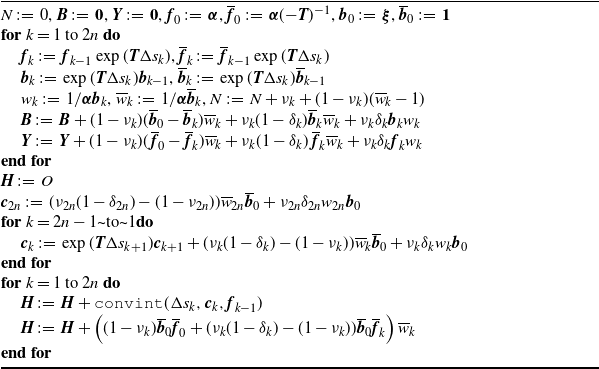
(4) \begin{align}\boldsymbol{c}_{2n} &= (\nu_{2n}(1-\delta_{2n})-(1-\nu_{2n})) \overline{w}_{2n} \overline{\boldsymbol{b}}_0 + \nu_{2n} \delta_{2n} w_{2n} \boldsymbol{b}_0, \\[-10pt] \nonumber \end{align}

(5) \begin{align}\boldsymbol{c}_k &= \exp(\boldsymbol{T} \Delta s_{k+1}) \boldsymbol{c}_{k+1} \nonumber\\[3pt]& \qquad + (\nu_{k}(1-\delta_{k})-(1-\nu_{k})) \overline{w}_{k} \overline{\boldsymbol{b}}_0 + \nu_{k} \delta_{k} w_{k} \boldsymbol{b}_0, \quad \text{for $k=2n-1, \ldots, 1$}. \end{align}

The derivation of (2)–(5) is provided in Appendix C.

Algorithm 1

E-step for PH distribution with LTRC data.

Algorithm 1 Long description

An equation representing the computation of matrix H. The equation starts with H equals the sum from k equals 1 to 2n of the integral from 0 to delta s sub k of the exponential of T u multiplied by c sub k multiplied by f sub k-1 multiplied by the exponential of T times the difference of delta s sub k and u with respect to du plus the sum from k equals 1 to 2n of the open parenthesis 1 minus nu sub k times b bar sub 0 times f bar sub 0 plus nu sub k times 1 minus delta sub k minus 1 minus nu sub k times b bar sub 0 times f bar sub k close parenthesis times w bar sub k. Here, w bar sub k equals 1 divided by alpha times b bar sub s sub k, delta s sub k equals s sub k minus s sub k-1, f sub k equals f of s sub k, f bar sub k equals f bar of s sub k, b sub k equals b of s sub k, and b bar sub k equals b bar of s sub k. The vector c sub k accumulates the future contributions required for computing H and is defined as the sum from l equals k to 2n of the exponential of T times the difference of s sub l and s sub k times the open parenthesis nu sub l times 1 minus delta sub l minus 1 minus nu sub l times w bar sub l times b bar sub 0 plus nu sub l times delta sub l times w sub l times b sub 0 close parenthesis for k equals 1 to 2n. Here, w sub k equals 1 divided by alpha times b of s sub k. This summation can be computed efficiently in reverse order using the recurrence c sub 2n equals nu sub 2n times 1 minus delta sub 2n minus 1 minus nu sub 2n times w bar sub 2n times b bar sub 0 plus nu sub 2n times delta sub 2n times w sub 2n times b sub 0 and c sub k equals the exponential of T times delta s sub k+1 times c sub k+1 plus nu sub k times 1 minus delta sub k minus 1 minus nu sub k times w bar sub k times b bar sub 0 plus nu sub k times delta sub k times w sub k times b sub 0 for k equals 2n-1 to 1.

We also define the quantities N, $\boldsymbol{B}$ , and $\boldsymbol{Y}$ as follows:

\begin{align*}& N = \sum_{k=1}^{2n} \nu_k + (1-\nu_k) (\overline{w}_k - 1), \\[2pt]& \boldsymbol{B} = \sum_{k=1}^{2n} (1-\nu_k) (\overline{\boldsymbol{b}}_0 - \overline{\boldsymbol{b}}_k) \overline{w}_k + \nu_k(1-\delta_k) \overline{\boldsymbol{b}}_k \overline{w}_k + \nu_k \delta_k \boldsymbol{b}_k w_k, \\[2pt]& \boldsymbol{Y} = \sum_{k=1}^{2n} (1-\nu_k) (\kern1.5pt \overline{\boldsymbol{f}}_0 - \overline{\boldsymbol{f}}_k) \overline{w}_k + \nu_k(1-\delta_k)\, \overline{\boldsymbol{f}}_k \overline{w}_k + \nu_k \delta_k\, \boldsymbol{f}_k w_k.\end{align*}

The computation algorithm for N, $\boldsymbol{B}$ , $\boldsymbol{Y}$ , and $\boldsymbol{H}$ is summarized in Algorithm 1. In this algorithm, ${\tt convint}(\Delta s_k, \boldsymbol{c}_k, \boldsymbol{f}_{k-1})$ denotes a function to compute the convolution of matrix exponential $\int_0^{\Delta s_k} \exp(\boldsymbol{T} u) \boldsymbol{c}_k \boldsymbol{f}_{k-1} \exp(\boldsymbol{T} (\Delta s_k -u)) \,\mathrm{d} u$ . Once all quantities are computed, the M-step updates are carried out as

\begin{align*} \alpha_i \, :\!= \, \frac{\alpha_i [\boldsymbol{B}]_i}{N}, \quad\xi_i \, :\!= \, \frac{[\boldsymbol{Y}]_i \xi_i}{[\boldsymbol{H}]_{i,i}}, \quad\lambda_{i,j} \, :\!= \, \frac{\lambda_{i,j} [\boldsymbol{H}]_{j,i}}{[\boldsymbol{H}]_{i,i}}. \end{align*}

Although Algorithm 1 provides a general computational framework, its overall performance critically depends on the efficient evaluation of the matrix-exponential convolution within the convint function. The next section describes an efficient computational procedure for evaluating this integral, with particular attention to sparse PH representations.

3.2. Canonical PH case

The primary computational bottleneck of the E-step in Algorithm 1 lies in evaluating the convolution integral, ${\tt convint}(t, \boldsymbol{x}, \boldsymbol{y})$ . Although existing approaches based on ordinary differential equations are available [Reference Asmussen, Nerman and Olsson5, Reference Olsson20], their $O(m^3)$ complexity makes them unsuitable for high-dimensional PH models. To address this limitation, we employ an efficient uniformization-based method [Reference Okamura, Dohi and Trivedi19], whose complexity scales with the number of non-zero elements in the generator matrix $\boldsymbol{T}$ .

The idea of this approach is to reorganize the convolution by observing that

\begin{align*} {\tt convint}(t,\boldsymbol{x},\boldsymbol{y})\, :\!= \, \int_0^{t} \exp(\boldsymbol{T} u)\, \boldsymbol{x}\, \boldsymbol{y}\, \exp\!\big(\boldsymbol{T}(t-u)\big)\,\mathrm{d} u \end{align*}

factorizes, at the integrand level, into the product of two terms, namely $\exp(\boldsymbol{T} u)\boldsymbol{x}$ and $\boldsymbol{y}\exp(\boldsymbol{T}(t-u))$ . This reorganization reduces the computational complexity from $O(m^3)$ to $O(m^2)$ even in the fully dense case. Moreover, since ${\tt convint}(\! \cdot \!)$ appears only through $\boldsymbol{H}(\! \cdot \!)$ and $\overline{\boldsymbol{H}}(\! \cdot \!)$ , entries (i, j) with $\lambda_{i,j}=0$ need not be computed. Consequently, the overall complexity becomes $O(\mathrm{nnz}(\boldsymbol{T}))$ , which scales linearly with the number of nonzero elements in $\boldsymbol{T}$ . A detailed description of algorithm is provided in [Reference Okamura, Dohi and Trivedi19].

The proposed algorithm becomes particularly effective when combined with the canonical representations of PH distributions. Canonical forms provide minimal parameterizations for acyclic PH distributions; in particular, any acyclic PH distribution can be transformed into equivalent canonical forms [Reference Cumani9]. Among the three canonical forms, we focus on canonical form 1 (CF1), which employs an upper bidiagonal generator matrix and reduces the number of free parameters to $2m-1$ :

\begin{align*}\boldsymbol{\alpha} = (\alpha_1,\ldots,\alpha_m), \quad\boldsymbol{T} = \begin{pmatrix}-\beta_1 &\quad \beta_1 &\quad &\quad \\&\quad \ddots &\quad \ddots &\quad \\&\quad &\quad -\beta_{m-1} &\quad \beta_{m-1} \\&\quad &\quad &\quad -\beta_m\end{pmatrix}, \quad\boldsymbol{\xi} = \begin{pmatrix}0 \\ \vdots \\ 0 \\ \beta_m\end{pmatrix},\end{align*}

where $0<\beta_1\le \cdots \le \beta_m$ . The structured (upper bidiagonal) form of CF1 simplifies parameter estimation and makes it particularly well suited for the efficient EM algorithm.

A key requirement of CF1 is that the diagonal elements must be ordered. This ordering both constrains the parameter space and enhances the numerical stability of the estimation process. An explicit bubble-sort-like procedure for enforcing this ordering is described in [Reference Okamura, Dohi and Trivedi19].

5.1. Comparative studies under right-censoring data

We compared the proposed algorithm with that of Olsson. Since Olsson’s method is not designed to handle left-truncated samples, we evaluated its performance using right-censored data generated by the following procedure.

Step I. Generate n failure times from a Weibull distribution with a shape parameter of 2 and a scale parameter of 1.

Step II. Generate n right-censoring times from an exponential distribution with a mean of 2.

Step III. For each pair, record the failure time as an observation if it occurs before the corresponding censoring time; otherwise, treat it as right-censored. Specifically, we considered the following datasets:

• • DS1 with 126 uncensored and 74 right-censored samples ( $n = 200$ );

• • DS2 with 668 uncensored and 332 right-censored samples ( $n = 1000$ ).

The numerical experiments were conducted on macOS Ventura, running on an Apple M2 chip with 16 GB of memory. We compared two implementations: the proposed algorithm, written in Julia (https://github.com/rellab/ph-experiments); and the fit function from the R package matrixdist (version 1.1.9) [Reference Bladt, Mueller and Yslas8], which serves as a current benchmark implementation of Olsson’s algorithm. In both implementations, the tolerance parameter of the uniformization method was set to $10^{-8}$ .

For each dataset, we evaluated performance across three distinct PH structures.

• • General PH: a dense (full) infinitesimal generator matrix.

• • Bidiagonal PH: an upper-bidiagonal generator matrix.

• • CF1: an upper-bidiagonal generator matrix with the additional constraint that the diagonal elements are ordered.

The number of phases m was varied over the set $\{5, 10, 20, 30, 50, 70, 100\}$ . To ensure a fair comparison, both algorithms were initialized with an identical set of parameters, obtained by running the matrixdist EM algorithm for five preliminary iterations.

The EM iterations were terminated when the change in the LLF over ten consecutive EM steps satisfied either a relative or an absolute tolerance criterion. Specifically, the algorithm was stopped if

\begin{align*}\frac{|\mathrm{LLF}_{\text{new}} - \mathrm{LLF}_{\text{old}}|}{|\mathrm{LLF}_{\text{old}}|} < 10^{-5} \quad \text{or} \quad |\mathrm{LLF}_{\text{new}} - \mathrm{LLF}_{\text{old}}| < 10^{-3}. \end{align*}

We report the total computation time (in seconds), the number of EM steps required for convergence, and the final LLF value.

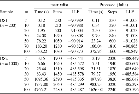
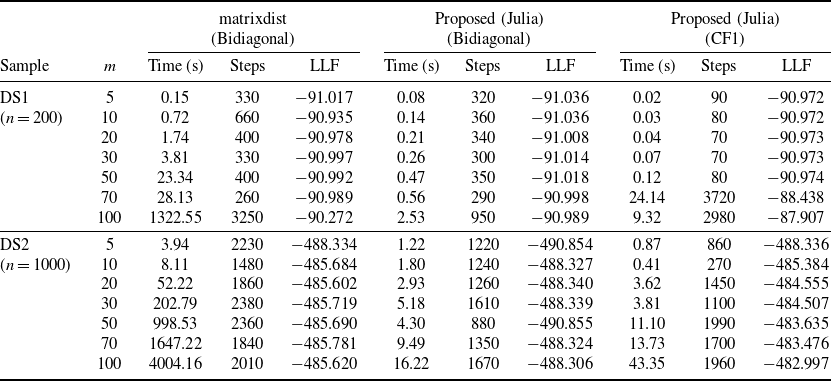
The numerical results, summarized in Tables 1 and 2, comprehensively validate our proposed algorithm. The CF1 run with $m=70$ is an outlier; we confirmed the runtime from the logs due to stiffness in later iterations. The most remarkable finding is the dramatic performance gain achieved by exploiting matrix sparsity. When fitting sparse models (bidiagonal and CF1), our proposed algorithm consistently outperforms the matrixdist package. This performance gap widens substantially as both the number of phases (m) and the sample size (n) increase. For instance, in the largest sparse case ( $n=1000$ , $m=100$ ), our CF1 implementation was over a factor of 92 faster than the comparable matrixdist Bidiagonal run. This confirms that our approach makes the estimation of high-dimensional PH distributions computationally tractable.

Table 1.

Comparison for general PH models on DS1 and DS2.

Table 1 Long description

A table comparing performance metrics for general PH models on two datasets, DS1 and DS2. The table has 14 rows and 10 columns. Column headers are Sample, m, matrixdist Time (s), matrixdist Steps, matrixdist LLF, Proposed (Julia) Time (s), Proposed (Julia) Steps, and Proposed (Julia) LLF. Row labels include DS1 (n=200) and DS2 (n=1000) with varying values of m from 5 to 100. Row 1: DS1, 5, 0.12, 230, -90.989, 0.11, 330, -91.003. Row 2: DS1, 10, 0.18, 210, -90.988, 0.34, 320, -91.001. Row 3: DS1, 20, 1.95, 500, -91.003, 2.50, 530, -91.023. Row 4: DS1, 30, 24.08, 1970, -90.808, 9.79, 840, -91.008. Row 5: DS1, 50, 76.22, 1050, -90.914, 23.24, 600, -91.028. Row 6: DS1, 70, 183.20, 1280, -90.829, 166.04, 1810, -90.865. Row 7: DS1, 100, 353.22, 1080, -90.873, 375.95, 1660, -90.849. Row 8: DS2, 5, 3.15, 1900, -488.441, 3.19, 2320, -488.449. Row 9: DS2, 10, 6.66, 1640, -485.572, 7.51, 1940, -485.607. Row 10: DS2, 20, 25.44, 1310, -485.598, 31.31, 1820, -485.649. Row 11: DS2, 30, 83.43, 1450, -485.578, 79.37, 1950, -485.584. Row 12: DS2, 50, 1095.36, 2590, -485.335, 497.93, 3820, -485.647. Row 13: DS2, 70, 1737.80, 2040, -485.299, 983.23, 3220, -485.398. Row 14: DS2, 100, 4766.21, 2280, -485.487, 1626.02, 2240, -485.596. The table compares the performance of the matrixdist package and the proposed Julia algorithm in terms of time (s), steps, and log-likelihood (LLF) for different sample sizes and values of m. Notable trends include the proposed Julia algorithm consistently outperforming the matrixdist package, especially as the number of phases (m) and sample size (n) increase.

Table 2.

Comparison for bidiagonal and CF1 PH models on DS1 and DS2.

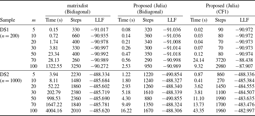
Table 2 Long description

The table compares the performance of matrixdist and proposed Julia algorithms for bidiagonal and CF1 PH models on datasets DS1 and DS2. It has 12 rows and 11 columns. The columns are labeled as Sample, m, Time (s), Steps, LLF for matrixdist (Bidiagonal), Time (s), Steps, LLF for Proposed (Julia) (Bidiagonal), and Time (s), Steps, LLF for Proposed (Julia) (CF1). The row labels include DS1 (n=200) and DS2 (n=1000) with varying values of m (5, 10, 20, 30, 50, 70, 100). Each row presents the time in seconds, steps, and log-likelihood (LLF) values for each method. Notable trends include the significant performance gain of the proposed Julia algorithm over matrixdist, especially as the number of phases (m) and sample size (n) increase. For instance, in the largest sparse case (n=1000, m=100), the proposed CF1 implementation is over a factor of 92 faster than the comparable matrixdist Bidiagonal run.

Beyond speed, the results highlight the significant role of the CF1 representation in achieving superior model fits. The unconstrained bidiagonal models tend to become trapped in poor local optima. In contrast, the ordering constraint of the CF1 structure effectively guides the optimization process toward solutions with substantially higher LLFs, especially for larger m. These findings demonstrate that the CF1 representation enhances not only computational efficiency but also the accuracy and stability of the final estimates.

5.2. Comparison of AIC and EIC

To evaluate the performance of AIC and EIC under LTRC data, synthetic datasets were generated according to the following procedure. For each of the n subjects, an LTRC sample was generated as follows. First, a potential right-censoring time $c_i$ was drawn from an exponential distribution with mean $1/\mu_1$ . Next, a Bernoulli trial with probability p determined whether the observation for subject i was left-truncated. If the observation was not truncated, a failure time $t_i$ was drawn from the original distribution f(t), and the truncation time was set to $\tau_i = 0$ . If the observation was left-truncated, a truncation time $\tau_i$ was drawn from an exponential distribution with mean $1/\mu_2$ , and a failure time $t_i$ was then drawn from the conditional distribution given survival beyond the truncation point, i.e. from the density $f(t)/S(\tau_i)$ for $t > \tau_i$ . In either case, the final observed time was $\min(t_i, c_i)$ , and the censoring indicator $\delta_i$ was set to 1 if $t_i \le c_i$ and 0 otherwise.

In the experiment, we considered three original distributions to generate LTRC samples of sizes $n = 200$ and $n = 1000$ .

• • Lognormal: a log-normal distribution with location parameter 1.0 and scale parameter 0.5.

• • Weibull: a Weibull distribution with shape parameter 5 and scale parameter 8.0.

• • Mixture: a mixture of the above log-normal and Weibull distributions, with mixing probability 0.3, which is the probability that a randomly selected observation comes from the log-normal distribution.

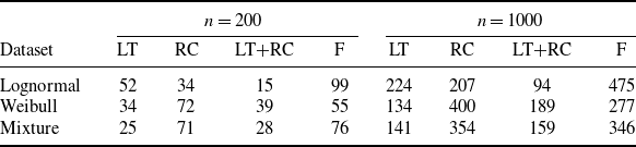
For all cases, the censoring and truncation parameters were set to $1/\mu_1 = 8.0$ , $1/\mu_2 = 1.0$ , and $p = 0.3$ . Table 3 summarizes the characteristics of the generated datasets.

Table 3.

Characteristics of the generated LTRC datasets.

Table 3 Long description

A table comparing characteristics of generated LTRC datasets for different sample sizes and distributions. The table has 3 rows and 8 columns. Column headers are: Dataset, LT, RC, LT+RC, F, LT, RC, LT+RC, F. Row labels are: Lognormal, Weibull, Mixture. Row 1: Lognormal, 52, 34, 15, 99, 224, 207, 94, 475. Row 2: Weibull, 34, 72, 39, 55, 134, 400, 189, 277. Row 3: Mixture, 25, 71, 28, 76, 141, 354, 159, 346. The table summarizes the number of left-truncated, right-censored, and failure samples for different datasets and sample sizes.

Note: LT, RC, and F denote the number of left-truncated, right-censored, and failure samples.

We conducted model fitting using the CF1 structure for each generated LTRC dataset, varying the number of phases m over $\{5, 10, 20, 30, 50, 70, 100\}$ . For each fitted model, both the AIC and EIC values were computed. The EIC was evaluated using $B = 200$ bootstrap samples. To further assess the goodness of fit of the estimated models, we calculated the cross-entropy (Cross) between the original failure-time distribution and the estimated CF1 model:

\begin{align*}H(f, f_{\mathrm{PH}}) = - \int f(t) \log f_{\mathrm{PH}}(t)\, \mathrm{d} t, \end{align*}

where f and $f_{\mathrm{PH}}$ denote the p.d.f.s of the original distribution and the estimated PH model, respectively. A smaller cross-entropy value indicates a closer fit to the original distribution. This serves as the benchmark for goodness of fit, as it directly measures the divergence from the original distribution.

Table 4.

Model selection results for Lognormal with $n=200$ and $n=1000$ .

Table 4 Long description

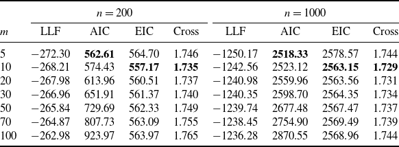
The table presents model selection results for Lognormal with sample sizes of 200 and 1000. It includes columns for Log-Likelihood (LLF), Akaike Information Criterion (AIC), EIC, and Cross-validation (Cross) for different values of m. The table is divided into two sections: one for n=200 and one for n=1000. Each section contains rows for m values of 5, 10, 20, 30, 50, 70, and 100. The values for LLF, AIC, EIC, and Cross are listed for each m value. For n=200, the LLF values range from -272.30 to -262.98, AIC values range from 562.61 to 923.97, EIC values range from 564.70 to 563.97, and Cross values range from 1.735 to 1.765. For n=1000, the LLF values range from -1250.17 to -1236.28, AIC values range from 2518.33 to 2870.55, EIC values range from 2578.57 to 2568.96, and Cross values range from 1.729 to 1.744.

Table 5.

Model selection results for Weibull with $n=200$ and $n=1000$ .

Table 5 Long description

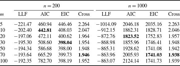
A table comparing model selection results for Weibull with sample sizes of 200 and 1000. The table has two main sections, one for each sample size. Each section contains columns for LLF, AIC, EIC, and Cross values, with rows labeled by different values of m (5, 10, 20, 30, 50, 70, 100). For n=200: Row 1: m, 5; LLF, -221.47; AIC, 460.94; EIC, 446.46; Cross, 2.264. Row 2: m, 10; LLF, -202.40; AIC, 442.81; EIC, 408.03; Cross, 2.047. Row 3: m, 20; LLF, -197.06; AIC, 472.11; EIC, 400.62; Cross, 1.964. Row 4: m, 30; LLF, -195.30; AIC, 508.60; EIC, 398.04; Cross, 1.954. Row 5: m, 50; LLF, -194.34; AIC, 586.68; EIC, 398.00; Cross, 1.948. Row 6: m, 70; LLF, -193.64; AIC, 665.29; EIC, 399.73; Cross, 1.946. Row 7: m, 100; LLF, -192.35; AIC, 782.70; EIC, 398.19; Cross, 1.952. For n=1000: Row 1: m, 5; LLF, -1014.09; AIC, 2046.18; EIC, 2035.16; Cross, 2.263. Row 2: m, 10; LLF, -912.15; AIC, 1862.31; EIC, 1828.71; Cross, 2.046. Row 3: m, 20; LLF, -872.76; AIC, 1823.52; EIC, 1752.83; Cross, 1.957. Row 4: m, 30; LLF, -868.98; AIC, 1855.96; EIC, 1746.41; Cross, 1.948. Row 5: m, 50; LLF, -865.31; AIC, 1928.62; EIC, 1741.08; Cross, 1.942. Row 6: m, 70; LLF, -863.96; AIC, 2005.93; EIC, 1741.03; Cross, 1.938. Row 7: m, 100; LLF, -863.07; AIC, 2124.14; EIC, 1741.73; Cross, 1.939.

Table 6.

Model selection results for Mixture with $n=200$ and $n=1000$ .

Table 6 Long description

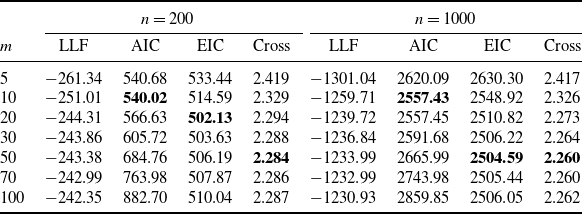
The table presents model selection results for Mixture with sample sizes of 200 and 1000. It is divided into two main sections based on the sample size: n=200 and n=1000. Each section contains columns for LLF, AIC, EIC, and Cross values, with rows labeled by different values of m (5, 10, 20, 30, 50, 70, 100). The table provides specific numerical values for each combination of m and sample size. For n=200, the values range from -261.34 to -242.35 for LLF, 540.68 to 882.70 for AIC, 533.44 to 510.04 for EIC, and 2.419 to 2.287 for Cross. For n=1000, the values range from -1301.04 to -1230.93 for LLF, 2620.09 to 2859.85 for AIC, 2630.30 to 2506.05 for EIC, and 2.417 to 2.262 for Cross. The table allows for a comparison of model performance across different sample sizes and values of m.

Tables 4–6. present the estimation results. The column labeled LLF indicates the maximum log-likelihood value, and the model selected by each criterion (i.e. that with the minimum value) is highlighted in bold. Figures 1(a)–(f) show the p.d.f.s of the original distributions and the CF1 models estimated under the AIC, EIC, and Cross.

Figure 1.

The p.d.f.s of the original and estimated CF1 models selected by AIC, EIC, and Cross: (a) Lognormal ( $n=200$ ); (b) Lognormal ( $n=1000$ ); (c) Weibull ( $n=200$ ); (d) Weibull ( $n=1000$ ); (e) Mixture ( $n=200$ ); (f) Mixture ( $n=1000$ ).

Figure 1 Long description

Six line graphs depict the probability density functions (p.d.f.s) of original and estimated CF1 models selected by AIC, EIC, and Cross for different distributions and sample sizes. Panel A: A line graph shows the probability density for a Lognormal distribution with a sample size of 200. The x-axis represents time (t) ranging from 0 to 10, and the y-axis represents probability density. The graph includes four lines: Original, AIC (m=5), EIC (m=10), and Cross (m=10). Panel B: A line graph shows the probability density for a Lognormal distribution with a sample size of 1000. The x-axis represents time (t) ranging from 0 to 10, and the y-axis represents probability density. The graph includes four lines: Original, AIC (m=5), EIC (m=10), and Cross (m=10). Panel C: A line graph shows the probability density for a Weibull distribution with a sample size of 200. The x-axis represents time (t) ranging from 0 to 15, and the y-axis represents probability density. The graph includes four lines: Original, AIC (m=10), EIC (m=30), and Cross (m=70). Panel D: A line graph shows the probability density for a Weibull distribution with a sample size of 1000. The x-axis represents time (t) ranging from 0 to 15, and the y-axis represents probability density. The graph includes four lines: Original, AIC (m=20), EIC (m=70), and Cross (m=70). Panel E: A line graph shows the probability density for a Mixture distribution with a sample size of 200. The x-axis represents time (t) ranging from 0 to 15, and the y-axis represents probability density. The graph includes four lines: Original, AIC (m=10), EIC (m=20), and Cross (m=50). Panel F: A line graph shows the probability density for a Mixture distribution with a sample size of 1000. The x-axis represents time (t) ranging from 0 to 15, and the y-axis represents probability density. The graph includes four lines: Original, AIC (m=10), EIC (m=50), and Cross (m=50).

A key finding from our experiments is that the EIC consistently outperforms the AIC in selecting models that more accurately capture the characteristics of the original distributions. This trend holds for both datasets with $n = 200$ and $n = 1000$ . In every case, the model selected by EIC achieved a lower cross-entropy score than the model selected by AIC. The visual evidence in Figure 1 clearly illustrates this performance gap. The most remarkable evidence comes from the Mixture dataset, which exhibits a bimodal structure. For both sample sizes, the AIC-selected model completely failed to capture this bimodal nature, whereas the EIC-selected model successfully reproduced both peaks, providing a qualitatively superior fit.

Furthermore, comparing the results between the $n = 200$ and $n = 1000$ datasets reveals a notable trend. For $n = 1000$ , the model selected by EIC perfectly matched the optimal model identified by the cross-entropy benchmark across all three cases. These results strongly suggest that EIC is a more robust and reliable criterion.