1. Introduction
The hydrostatic two-dimensional (single-layer) shallow-water (SW) model has long been used to study shallow free-surface flows of uniform density held down by gravity, with or without the effects of background rotation (see Saint-Venant Reference Saint-Venant1871; Gill Reference Gill1982; Vallis Reference Vallis2008). The SW model reduces the parent three-dimensional (3-D) model for a fluid of uniform density by making the hydrostatic approximation (neglecting the vertical acceleration) and assuming the horizontal flow is independent of height. This is justified for long waves, i.e. when horizontal scales of motion are large compared with the fluid height. A generalisation of the SW model known as the Green–Naghdi (GN) model (see Green, Laws & Naghdi Reference Green, Laws and Naghdi1974; Green & Naghdi Reference Green and Naghdi1976; Ertekin Reference Ertekin1984; Miles & Salmon Reference Miles and Salmon1985; Holm Reference Holm1988; Demirbilek & Webster Reference Demirbilek, Webster and Herbich1999; Dellar Reference Dellar2003; Dellar & Salmon Reference Dellar and Salmon2005; Dutykh et al. Reference Dutykh, Clamond, Milewski and Mitsotakis2013; Dritschel & Jalali Reference Dritschel and Jalali2019, and references therein) relaxes the hydrostatic approximation but retains the assumption that the horizontal flow is independent of height (note: we consider only the first (lowest) level in a hierarchy of GN models, see Shields & Webster (Reference Shields and Webster1988), Demirbilek & Webster (Reference Demirbilek, Webster and Herbich1999)). Historically, in fact Serre (Reference Serre1953) was the first to derive the equations, which were re-discovered by Su & Gardner (Reference Su and Gardner1969).
The relaxation of the hydrostatic approximation in the GN model results in a considerably more complicated set of equations, as the additional terms involving the non-hydrostatic acceleration depend on time derivatives of the velocity field  ${{\boldsymbol {u}}}$, making the model implicit in
 ${{\boldsymbol {u}}}$ (see Pearce & Esler Reference Pearce and Esler2010; Dritschel & Jalali Reference Dritschel and Jalali2019, and references therein). An alternative explicit formulation of the model uses a momentum variable
 ${{\boldsymbol {m}}}$, from which
 ${{\boldsymbol {u}}}$ is found from a linear elliptic equation (Holm Reference Holm1988; Dellar Reference Dellar2003; Dellar & Salmon Reference Dellar and Salmon2005; Le Métayer, Gavrilyuk & Hank Reference Le Métayer, Gavrilyuk and Hank2010; Dutykh et al. Reference Dutykh, Clamond, Milewski and Mitsotakis2013). Below, we show that in fact there is another, arguably simpler, alternative: just vertically average the parent 3-D model and deduce the (scalar) non-hydrostatic pressure from a linear elliptic equation.
The vast majority of previous works have applied the GN model to non-rotating flows, often in one spatial dimension, and have demonstrated the often significantly greater accuracy of the GN model over the SW one, for both linear and nonlinear flows. To our knowledge, Pearce & Esler (Reference Pearce and Esler2010) were the first to consider rotating flows, of relevance to geophysical fluid dynamics. Here, we extend that study by comparing the GN and SW models with their parent 3-D model for rotating free-surface flows at moderate Rossby and Froude numbers characteristic of atmospheric and oceanic flows (cf. Vallis Reference Vallis2008). The following section reviews the parent 3-D model and briefly describes the numerical approach used (details may be found in the appendices). Section 3 revisits the two-dimensional (2-D) SW and GN models, and in particular derives a new explicit reformulation of the GN model in which the non-hydrostatic pressure is diagnosed from a simple, linear, and robustly convergent elliptic equation. Section 4 presents the main results. There, we examine a highly nonlinear example of shear instability, initialised as a height-independent flow in the 3-D simulation. The initial, variable free-surface height is found by ‘balance’ to reduce the initial gravity-wave generation as in Dritschel & Jalali (Reference Dritschel and Jalali2019) (hereafter DJ19). The 2-D models use identical initial conditions (albeit for one layer). The models also use identical numerical formulations in order to isolate the physical differences between them. Our conclusions are offered in § 5.
2. Mathematical and numerical approach
We consider a 3-D inviscid incompressible fluid of uniform density  $\rho$ in a frame of reference rotating uniformly about the
 $z$ axis at the rate
 $\Omega =f/2$ (
 $\,f$ is known as the Coriolis frequency in the geophysical context). The fluid is taken to lie above a flat bottom at
 $z=0$ and have a local variable height
 $h({{\boldsymbol {x}}},t)$, where
 ${{\boldsymbol {x}}}=(x,y)$ is the horizontal position vector and
 $t$ is time. Gravity acts downwards. The fluid motion is governed by Euler's equations,
 \begin{gather} \frac{{\textrm{D}} {u}}{{\textrm{D}} {t}}-fv ={-}\frac{{{\partial}} {P}}{{{\partial}} {x}}, \end{gather}
 \begin{gather} \frac{{\textrm{D}} {v}}{{\textrm{D}} {t}}+fu ={-}\frac{{{\partial}} {P}}{{{\partial}} {y}}, \end{gather}
 \begin{gather} \frac{{\textrm{D}} {w}}{{\textrm{D}} {t}} ={-}\frac{{{\partial}} {P}}{{{\partial}} {z}} - g, \end{gather}
 \begin{gather} \frac{{{\partial}} {u}}{{{\partial}} {x}}+\frac{{{\partial}} {v}}{{{\partial}} {y}}+\frac{{{\partial}} {w}}{{{\partial}} {z}} = 0, \end{gather}
in Cartesian coordinates, where  ${\textrm {D}}/{\textrm {D}}{t}={{\partial }}/{{\partial }}{t}+u{{\partial }}/{{\partial }}{x}+v{{\partial }}/{{\partial }}{y}+w{{\partial }}/{{\partial }}{z}$ is the material derivative,
 $(u,v,w)$ is the velocity field,
 $P=p/\rho$ is the pressure scaled by the constant density and
 $g$ is the acceleration due to gravity. The boundary conditions are
 \begin{gather} w = 0 \quad\text{at}\ z=0, \end{gather}
 \begin{gather} w = \frac{{{\partial}} {h}}{{{\partial}} {t}}+u\frac{{{\partial}} {h}}{{{\partial}} {x}}+v\frac{{{\partial}} {h}}{{{\partial}} {y}} \quad\text{at}\ z=h, \end{gather}
 \begin{gather} \frac{{{\partial}} {P}}{{{\partial}} {z}} ={-}g \quad\text{at}\ z=0, \end{gather}
and
 \begin{equation} P = 0 \quad\text{at}\ z=h. \end{equation}
We consider only periodic boundaries in  $x$ and in
 $y$. While the (scaled) pressure can take any constant value at the free surface, without loss of generality we have taken
 $P=0$ there.
2.1. A coordinate transformation using a material vertical coordinate
To facilitate the numerical solution of these equations, we introduce a change in the vertical coordinate from  $z$ to the material coordinate
 ${{\theta }}$ (satisfying
 ${\textrm {D}}{{\theta }}/{\textrm {D}}{t}=0$), where
 ${{\theta }}$ is taken to vary from
 $0$ at
 $z=0$, to the mean fluid height
 $H$ (constant), at
 $z=h({{\boldsymbol {x}}},t)$. The height of the coordinate surface
 ${{\theta }}=$ constant is denoted by
 $z=\mathscr {z}(x,y,{{\theta }},t)$. The ‘thickness’
 ${{\partial }}\mathscr {z}/{{\partial }}{{\theta }}$ is denoted by
 ${{\rho _\theta }}$. Note: we tacitly assume that these material coordinate surfaces do not overturn (i.e. that
 $\mathscr {z}(x,y,{{\theta }},t)$ remains single valued over
 ${{\theta }}$). Thus, the numerical model can only be applied to such ‘regular’ flows, but in practice this appears not to be a restriction when modelling flows having low to moderate Rossby and Froude numbers, as here. We find no evidence of shock formation in the results presented below and in many additional simulations using this method.
To transform equations (2.1)–(2.4) to  ${{\theta }}$ coordinates, we make use of the following identities:
 \begin{equation} \frac{{{\partial}} {F}}{{{\partial}} {z}} = \frac{1}{{{\rho_\theta}}}\,\frac{{{\partial}} {F}}{{{\partial}} {{{\theta}}}}, \end{equation}
together with
 \begin{equation} \left.\frac{{{\partial}} {F}}{{{\partial}} {x}}\right|_z = \frac{{{\partial}} {F}}{{{\partial}} {x}}-\frac{1}{{{\rho_\theta}}}\,\frac{{{\partial}} {F}}{{{\partial}} {{{\theta}}}}\,\frac{{{\partial}} {\mathscr{z}}}{{{\partial}} {x}} \quad \text{and} \quad \left.\frac{{{\partial}} {F}}{{{\partial}} {y}}\right|_z = \frac{{{\partial}} {F}}{{{\partial}} {y}}-\frac{1}{{{\rho_\theta}}}\,\frac{{{\partial}} {F}}{{{\partial}} {{{\theta}}}}\,\frac{{{\partial}} {\mathscr{z}}}{{{\partial}} {y}}, \end{equation}
for any scalar field  $F$. The vertical bar on the left in (2.10a,b) indicates that horizontal derivatives are taken holding
 $z$ fixed. Otherwise, they are taken holding
 ${{\theta }}$ fixed, as on the right.
The horizontal momentum equations (2.1) and (2.2) then transform to
 \begin{gather} D{u}-fv ={-}\frac{{{\partial}} {P}}{{{\partial}} {x}}+\frac{1}{{{\rho_\theta}}} \,\frac{{{\partial}} {P}}{{{\partial}} {{{\theta}}}}\,\frac{{{\partial}} {\mathscr{z}}}{{{\partial}} {x}}, \end{gather}
 \begin{gather} D{v}+fu ={-}\frac{{{\partial}} {P}}{{{\partial}} {y}}+\frac{1}{{{\rho_\theta}}}\,\frac{{{\partial}} {P}}{{{\partial}} {{{\theta}}}}\,\frac{{{\partial}} {\mathscr{z}}}{{{\partial}} {y}}, \end{gather}
where  $D={{\partial }}/{{\partial }}{t}+u{{\partial }}/{{\partial }}{x}+v{{\partial }}/{{\partial }}{y}$. Conservation of mass, or volume due to incompressibility (2.4), implies
 \begin{equation} \frac{{{\partial}} {{{\rho_\theta}}}}{{{\partial}} {t}}+\frac{{{\partial}} {}}{{{\partial}} {x}}(u{{\rho_\theta}})+\frac{{{\partial}} {}}{{{\partial}} {y}}(v{{\rho_\theta}})=0 , \end{equation}
which is an evolution equation for the layer thickness  ${{\rho _\theta }}$. In
 ${{\theta }}$ coordinates, both the coordinate surface height
 $\mathscr {z}$ and the vertical velocity
 $w$ are diagnosed from the thickness
 ${{\rho _\theta }}$
 \begin{gather} \mathscr{z}(x,y,{{\theta}},t) = \int_{0}^{{{\theta}}}{{\rho_\theta}}(x,y,s,t)\,{\textrm{d}}{s}, \end{gather}
 \begin{gather} w(x,y,{{\theta}},t) = D\mathscr{z} = u\frac{{{\partial}} {\mathscr{z}}}{{{\partial}} {x}}+v\frac{{{\partial}} {\mathscr{z}}}{{{\partial}} {y}}- \int_{0}^{{{\theta}}}\left(\frac{{{\partial}} {}}{{{\partial}} {x}}(u{{\rho_\theta}})+\frac{{{\partial}} {}}{{{\partial}} {y}}(v{{\rho_\theta}})\right)\,{\textrm{d}}{s} , \end{gather}
using (2.13). The free-surface height  $h$ is given by
 $\mathscr {z}$ at
 ${{\theta }}=H$, i.e.
 $h(x,y,t)=\mathscr {z}(x,y,H,t)$.
Notice that the prognostic variables in  ${{\theta }}$ coordinates are
 $u$,
 $v$ and
 ${{\rho _\theta }}$ rather than
 $u$,
 $v$ and
 $w$ in Cartesian coordinates. The derivation of the above equations also follows directly from the standard isopycnal (constant density) or isentropic (constant entropy) coordinate formulation used in geophysical fluid dynamics (Pedlosky Reference Pedlosky1987).
The pressure  $P$ must also be diagnosed in this formulation in order to calculate the horizontal velocity tendencies in (2.11) and (2.12). The diagnostic equation is found by first taking the divergence of the original momentum equations (2.1)–(2.3) in Cartesian coordinates giving
 \begin{equation} \left.\boldsymbol{\nabla}_3^{2}\right|_z P=\left.f\zeta\right|_z-\left.\boldsymbol{\nabla}_3\right|_z\boldsymbol{\cdot} \left(\left.{{\boldsymbol{u}}}_3\boldsymbol{\cdot}\boldsymbol{\nabla}_3\right|_z\,{{\boldsymbol{u}}}_3\right), \end{equation}
where  $\boldsymbol{\nabla}_3^{2}|_z$ is the 3-D Laplace operator in
 $z$ coordinates,
 $\boldsymbol {\nabla }_3$ is the 3-D gradient operator,
 ${{\boldsymbol {u}}}_3=(u,v,w)$ is the 3-D velocity field and
 $\zeta |_z$ is the vertical vorticity
 \begin{equation} \left.\zeta\right|_z=\left.\frac{{{\partial}} {v}}{{{\partial}} {x}}\right|_z-\left.\frac{{{\partial}} {u}}{{{\partial}} {y}}\right|_z =\frac{{{\partial}} {v}}{{{\partial}} {x}}-\frac{1}{{{\rho_\theta}}}\frac{{{\partial}} {v}}{{{\partial}} {{{\theta}}}}\,\frac{{{\partial}} {\mathscr{z}}}{{{\partial}} {x}}-\frac{{{\partial}} {u}}{{{\partial}} {y}} +\frac{1}{{{\rho_\theta}}}\frac{{{\partial}} {u}}{{{\partial}} {{{\theta}}}}\,\frac{{{\partial}} {\mathscr{z}}}{{{\partial}} {y}}, \end{equation}
after converting to  ${{\theta }}$ coordinates. Likewise, the nonlinear term in (2.16) may be written
 \begin{equation} \left.\boldsymbol{\nabla}_3\right|_z\boldsymbol{\cdot}\left(\left.{{\boldsymbol{u}}}_3\boldsymbol{\cdot}\boldsymbol{\nabla}_3\right|_z\,{{\boldsymbol{u}}}_3\right)={-}2\left[\left.J_{xy}(u,v)\right|_z+ \left.J_{yz}(v,w)\right|_z+ \left. J_{zx}(w,u)\right|_z\right], \end{equation}
where
 \begin{equation} \left. J_{ab}(F,G)\right|_z=\left.\frac{{{\partial}} {F}}{{{\partial}} {a}}\right|_z\left.\frac{{{\partial}} {G}}{{{\partial}} {b}}\right|_z -\left.\frac{{{\partial}} {F}}{{{\partial}} {b}}\right|_z\left.\frac{{{\partial}} {G}}{{{\partial}} {a}}\right|_z, \end{equation}
is the Jacobian of two scalar fields  $F$ and
 $G$ with respect to any two Cartesian coordinates ‘
 $a$’ and ‘
 $b$’ (the vertical bar is absent when either
 $a$ or
 $b$ equals
 $z$). Using the coordinate transformation in (2.9) and (2.10a,b), we find
 \begin{gather} \left.J_{xy}(u,v)\right|_z = J_{xy}(u,v) +J_{y{{\theta}}}(u,v)\frac{{{\partial}} {\mathscr{z}}}{{{\partial}} {x}} +J_{{{\theta}}x}(u,v)\frac{{{\partial}} {\mathscr{z}}}{{{\partial}} {y}}, \end{gather}
 \begin{gather} \left.J_{yz}(v,w)\right|_z = J_{y{{\theta}}}(v,w), \end{gather}
 \begin{gather} \left.J_{zx}(w,u)\right|_z = J_{{{\theta}}x}(w,u), \end{gather}
where
 \begin{gather} J_{xy}(F,G) = \frac{{{\partial}} {F}}{{{\partial}} {x}}\frac{{{\partial}} {G}}{{{\partial}} {y}}-\frac{{{\partial}} {F}}{{{\partial}} {y}}\frac{{{\partial}} {G}}{{{\partial}} {x}}, \end{gather}
 \begin{gather} J_{y{{\theta}}}(F,G) = \frac{1}{{{\rho_\theta}}}\left(\frac{{{\partial}} {F}}{{{\partial}} {y}}\frac{{{\partial}} {G}}{{{\partial}} {{{\theta}}}}-\frac{{{\partial}} {F}}{{{\partial}} {{{\theta}}}}\frac{{{\partial}} {G}}{{{\partial}} {y}}\right), \end{gather}
 \begin{gather} J_{{{\theta}}x}(F,G) = \frac{1}{{{\rho_\theta}}}\left(\frac{{{\partial}} {F}}{{{\partial}} {{{\theta}}}}\frac{{{\partial}} {G}}{{{\partial}} {x}}-\frac{{{\partial}} {F}}{{{\partial}} {x}}\frac{{{\partial}} {G}}{{{\partial}} {{{\theta}}}}\right) . \end{gather}
The Laplacian of the pressure in (2.16) may similarly be transformed using
 \begin{equation} \left.\boldsymbol{\nabla}_3^{2}\right|_z P=\left.\frac{{{\partial}} {}}{{{\partial}} {x}}\right|_z\left(\frac{{{\partial}} {P}}{{{\partial}} {x}} -\frac{1}{{{\rho_\theta}}}\frac{{{\partial}} {P}}{{{\partial}} {{{\theta}}}}\,\frac{{{\partial}} {\mathscr{z}}}{{{\partial}} {x}}\right) +\left.\frac{{{\partial}} {}}{{{\partial}} {y}}\right|_z\left(\frac{{{\partial}} {P}}{{{\partial}} {y}} -\frac{1}{{{\rho_\theta}}}\frac{{{\partial}} {P}}{{{\partial}} {{{\theta}}}}\,\frac{{{\partial}} {\mathscr{z}}}{{{\partial}} {y}}\right) +\frac{{{\partial}} {}}{{{\partial}} {z}}\left(\frac{1}{{{\rho_\theta}}}\frac{{{\partial}} {P}}{{{\partial}} {{{\theta}}}}\right), \end{equation}
followed by a second application of the transformation rules in (2.9) and (2.10a,b). After dividing the pressure into a hydrostatic part  $P_h=g(h-\mathscr {z}(x,y,{{\theta }},t))$ and a remaining non-hydrostatic part
 ${{\tilde {P}}}=P-P_h$, we obtain the diagnostic equation satisfied by
 ${{\tilde {P}}}$
 \begin{equation} \boldsymbol{\nabla}^{2}{{\tilde{P}}}+\frac{\partial^{2}{{{\tilde{P}}}}}{\partial{{{\theta}}}^{2}} =S_0+{{\boldsymbol{\sigma}}}\boldsymbol{\cdot}\boldsymbol{\nabla}\frac{{{\partial}} {{{\tilde{P}}}}}{{{\partial}} {{{\theta}}}} +\frac{1}{2}\left(\frac{{{\partial}} {\tau}}{{{\partial}} {{{\theta}}}}+\boldsymbol{\nabla}\boldsymbol{\cdot}{{\boldsymbol{\sigma}}}\right)\frac{{{\partial}} {{{\tilde{P}}}}}{{{\partial}} {{{\theta}}}} +\tau\frac{\partial^{2}{{{\tilde{P}}}}}{\partial{{{\theta}}}^{2}}, \end{equation}
where  $\boldsymbol {\nabla }$ in the two-dimensional gradient operator,
 $\boldsymbol{\nabla} ^{2}=\boldsymbol {\nabla }\boldsymbol {\cdot }\boldsymbol {\nabla }$,
 \begin{equation} {{\boldsymbol{\sigma}}}= \frac{2}{{{\rho_\theta}}}\boldsymbol{\nabla}\mathscr{z}, \quad \tau=1-\frac{1}{{{\rho_\theta}}^{2}}-\frac{1}{4}\|{{\boldsymbol{\sigma}}}\|^{2} , \end{equation}
and where we have kept the constant-coefficient parts on the left-hand side. The ‘source’ term  $S_0$, which is independent of
 ${{\tilde {P}}}$, is given by
 \begin{align} S_0&=f\left(\frac{{{\partial}} {v}}{{{\partial}} {x}}-\frac{1}{{{\rho_\theta}}}\frac{{{\partial}} {v}}{{{\partial}} {{{\theta}}}}\frac{{{\partial}} {\mathscr{z}}}{{{\partial}} {x}}-\frac{{{\partial}} {u}}{{{\partial}} {y}} +\frac{1}{{{\rho_\theta}}}\frac{{{\partial}} {u}}{{{\partial}} {{{\theta}}}}\,\frac{{{\partial}} {\mathscr{z}}}{{{\partial}} {y}}\right)-g\boldsymbol{\nabla}^{2}{h} \nonumber\\ &\qquad +2\left(J_{xy}(u,v)+J_{y{{\theta}}}(u,v)\frac{{{\partial}} {\mathscr{z}}}{{{\partial}} {x}} +J_{{{\theta}}x}(u,v)\frac{{{\partial}} {\mathscr{z}}}{{{\partial}} {y}}+J_{y{{\theta}}}(v,w)+J_{{{\theta}}x}(w,u)\right) . \end{align}
In practice, the linear equation (2.27) for  ${{\tilde {P}}}$ is solved iteratively (see appendix A for details).
2.2. The 3-D equations in  $({q_l},\delta ,\gamma _l)$ variables

In rotating stratified flows, it has proved advantageous both theoretically and numerically to employ an alternative set of prognostic variables which represent the underlying geostrophic and hydrostatic balance in rapidly rotating, strongly stratified flows (see DJ19 and references therein). Geostrophic balance means that the horizontal acceleration is negligible compared with the Coriolis acceleration, while hydrostatic balance means that the vertical acceleration is negligible compared with gravity. The relative sizes of these accelerations compared with rotation and gravity are measured by the Rossby number and the Froude number, respectively (Vallis Reference Vallis2008).
The prognostic variable set which has proved particularly useful consists of the Rossby–Ertel potential vorticity (PV)
 \begin{equation} q=\left.{{\boldsymbol{\omega}}}_a\right|_z\boldsymbol{\cdot}\left.\boldsymbol{\nabla}_3\right|_z({{\theta}}/H) =(\left.{{\boldsymbol{\omega}}}\right|_z+f{{\boldsymbol{k}}})\boldsymbol{\cdot}\left.\boldsymbol{\nabla}_3\right|_z({{\theta}}/H), \end{equation}
where  ${{\boldsymbol {\omega }}}|_z=\boldsymbol {\nabla }_3|_z\times {{\boldsymbol {u}}}_3$ is the vector vorticity and
 ${{\boldsymbol {k}}}$ is the vertical unit vector, the horizontal divergence of the velocity field
 \begin{equation} \delta=\boldsymbol{\nabla}\boldsymbol{\cdot}{{\boldsymbol{u}}}, \end{equation}
where  ${{\boldsymbol {u}}}=(u,v)$, and the horizontal divergence of the horizontal acceleration field
 \begin{equation} \gamma=\boldsymbol{\nabla}\boldsymbol{\cdot}(D{{\boldsymbol{u}}}), \end{equation}
(Mohebalhojeh & Dritschel Reference Mohebalhojeh and Dritschel2001; Smith & Dritschel Reference Smith and Dritschel2006; Mohebalhojeh & Dritschel Reference Mohebalhojeh and Dritschel2007; Dritschel, Gottwald & Oliver Reference Dritschel, Gottwald and Oliver2017). In (2.30),  ${{\boldsymbol {\omega }}}_a|_z$ is the absolute vorticity as seen in the original, non-rotating reference frame. Because
 ${{\theta }}$ is a material coordinate (
 ${\textrm {D}}{{\theta }}/ {\textrm {D}}{t}=0$), it follows that
 $q$ is materially conserved (
 ${\textrm {D}}{q}/{\textrm {D}}{t}=0$), a result originally due to Beltrami (Reference Beltrami1871) (see also Viúdez Reference Viúdez2001).
For the full non-hydrostatic 3-D equations considered here, these variables result in complicated ‘inversion relations’ (nonlinear elliptic equations) for the recovery of  $u$,
 $v$ and
 ${{\rho _\theta }}$ from
 $q$,
 $\delta$ and
 $\gamma$. We instead use linearised approximations to
 $q$ and
 $\gamma$ defined respectively as
 \begin{equation} {q_l}=\zeta-f{{\tilde{\rho}_\theta}} \quad\text{and}\quad \gamma_l=f\zeta-c^{2}\boldsymbol{\nabla}^{2}\,{{\tilde{h}}}, \end{equation}
where  $\zeta ={{\partial }}{v}/{{\partial }}{x}-{{\partial }}{u}/{{\partial }}{y}$ is the relative vorticity in
 ${{\theta }}$ coordinates,
 ${{\tilde {\rho }_\theta }}={{\rho _\theta }}-1$ is the thickness anomaly (with zero horizontal mean),
 $c^{2}=gH$ is a characteristic squared surface gravity-wave speed and
 \begin{equation} {{\tilde{h}}}(x,y,t)=\frac{h-H}{H}=\frac{1}{H}\int_{0}^{H}{{\tilde{\rho}_\theta}}(x,y,{{\theta}},t)\,{\textrm{d}}{{{\theta}}}, \end{equation}
is the dimensionless height anomaly. Note that taking the mean thickness to be unity ensures that the mean height  $h$ is
 $H$, see (2.14).
The evolution equations for these new prognostic variables are readily recovered from (2.11), (2.12) and (2.13), the latter rewritten here in terms of  ${{\tilde {\rho }_\theta }}$ as
 \begin{equation} \frac{{{\partial}} {{{\tilde{\rho}_\theta}}}}{{{\partial}} {t}}+\boldsymbol{\nabla}\boldsymbol{\cdot}\left((1+{{\tilde{\rho}_\theta}}){{\boldsymbol{u}}}\right)=0, \end{equation}
after differentiation. The result is
 \begin{gather} \frac{{{\partial}} {{q_l}}}{{{\partial}} {t}} ={-}\boldsymbol{\nabla}\boldsymbol{\cdot}\left({q_l}{{\boldsymbol{u}}}\right)-J_{xy}(a_z,\mathscr{z}), \end{gather}
 \begin{gather} \frac{{{\partial}} {\delta}}{{{\partial}} {t}}-\gamma_l ={-}\boldsymbol{\nabla}\boldsymbol{\cdot}\left(\delta{{\boldsymbol{u}}}\right) +2J_{xy}(u,v)-\boldsymbol{\nabla}^{2}{{\tilde{P}}}-\boldsymbol{\nabla}\boldsymbol{\cdot}\left(a_z\boldsymbol{\nabla}\mathscr{z}\right), \end{gather}
 \begin{gather} \frac{{{\partial}} {\gamma_l}}{{{\partial}} {t}}-\mathbb{G}\delta ={-}f\left[\boldsymbol{\nabla}\boldsymbol{\cdot}\left({q_l}{{\boldsymbol{u}}}\right)+J_{xy}(a_z,\mathscr{z})\right] +\mathbb{G}\boldsymbol{\nabla}\boldsymbol{\cdot}\left({{\tilde{\rho}_\theta}}{{\boldsymbol{u}}}\right), \end{gather}
where
 \begin{equation} a_z={-}\frac{1}{{{\rho_\theta}}}\,\frac{{{\partial}} {{{\tilde{P}}}}}{{{\partial}} {{{\theta}}}}, \end{equation}
is the vertical acceleration and the gravity-wave operator  $\mathbb {G}$ is defined through
 \begin{equation} \mathbb{G}\xi\equiv c^{2}\boldsymbol{\nabla}^{2}\left[\frac{1}{H}\int_{0}^{H}\xi(x,y,s,t)\,{\textrm{d}}{s}\right] -f^{2}\xi(x,y,{{\theta}},t), \end{equation}
for any field  $\xi$. Thus,
 $c^{2}\boldsymbol{\nabla} ^{2}$ operates on the
 ${{\theta }}$ average of
 $\xi$ only.
2.3. Inversion
The set of prognostic variables  $({q_l},\delta ,\gamma _l)$ leads to a particularly simple way of recovering the horizontal velocity field
 ${{\boldsymbol {u}}}$ and the thickness anomaly
 ${{\tilde {\rho }_\theta }}$. The definitions of the prognostic variables in (2.31) and (2.33a,b) depend on
 $u$,
 $v$ and
 ${{\tilde {\rho }_\theta }}$ in a linear way, and moreover with constant coefficients.
The first step is to decompose the horizontal velocity field into a mean part  ${{\boldsymbol {U}}}=(U(t),V(t))$, a non-divergent part and divergent part, respectively expressed in terms of a streamfunction
 $\psi$ and a potential
 $\chi$
 \begin{equation} u=U-\frac{{{\partial}} {\psi}}{{{\partial}} {y}}+\frac{{{\partial}} {\chi}}{{{\partial}} {x}};\quad v=V+\frac{{{\partial}} {\psi}}{{{\partial}} {x}}+\frac{{{\partial}} {\chi}}{{{\partial}} {y}}. \end{equation}
Using the definition of the vorticity  $\zeta$ and the divergence
 $\delta$, we obtain Poisson equations for
 $\psi$ and
 $\chi$
 \begin{equation} \boldsymbol{\nabla}^{2}\psi=\zeta ;\quad \boldsymbol{\nabla}^{2}\chi=\delta , \end{equation}
which are readily solved on each coordinate surface  ${{\theta }}=$ constant after a horizontal spectral transform in the doubly periodic domain considered. However,
 $\zeta$ is not one of the new prognostic variables, but from (2.33a,b) involves
 ${q_l}$ and
 ${{\tilde {\rho }_\theta }}$ through
 $\zeta ={q_l}+f{{\tilde {\rho }_\theta }}$. Moreover,
 ${{\tilde {\rho }_\theta }}$ is also not one of the new variables, but the definition of
 $\gamma _l$ provides a simple elliptic equation to find
 ${{\tilde {\rho }_\theta }}$
 \begin{equation} \mathbb{G}{{\tilde{\rho}_\theta}}=f{q_l}-\gamma_l, \end{equation}
which is again readily solved after a horizontal spectral transform (the operator  $\mathbb {G}$ is defined in (2.40)). If we define
 $\eta =\gamma _l/f^{2}-{q_l}/f$, the formal solution is
 \begin{equation} {{\tilde{\rho}_\theta}}=\eta(k_x,k_y,{{\theta}},t)-\frac{c^{2}k^{2}}{f^{2}+c^{2}k^{2}}\, \frac{1}{H}\int_{0}^{H}\eta(k_x,k_y,s,t)\,{\textrm{d}}{s}, \end{equation}
in spectral space where  $-\boldsymbol{\nabla} ^{2}\to k^2 = k_x^2+k_y^2$, the squared horizontal wavenumber. In practice, the integral is calculated using the trapezoidal integration formula (see appendix B).
Once  ${{\tilde {\rho }_\theta }}$ is thereby obtained, we find
 $\zeta ={q_l}+f{{\tilde {\rho }_\theta }}$ and thus the streamfunction
 $\psi$ by (2.42a,b). The remaining issue is the mean horizontal flow
 $(U(t),V(t))$. As in DJ19, we find this by requiring that the (relative) horizontal momentum vanishes
 \begin{equation} \langle{{\rho_\theta}}{{\boldsymbol{u}}}\rangle=0 \quad\Rightarrow\quad {{\boldsymbol{U}}}={-}\langle{{\tilde{\rho}_\theta}}\tilde{{{\boldsymbol{u}}}}\rangle, \end{equation}
where  $\tilde {{{\boldsymbol {u}}}}$ is the horizontal velocity field excluding its mean part and
 $\langle \cdot \rangle$ denotes a domain average (over
 $x$,
 $y$ and
 ${{\theta }}$). We show next that the (relative) horizontal momentum remains zero if initially zero.
2.4. Conservation
The original equations conserve mass, energy, horizontal momentum and (if the domain possesses circular symmetry) angular momentum. The change of coordinates from  $z$ to
 ${{\theta }}$ preserves this conservation but alters the forms of the conserved quantities.
The total mass (or volume here for an incompressible fluid) in any given layer between material coordinate surfaces  ${{\theta }}$ and
 ${{\theta }}+{\textrm {d}}{{\theta }}$ is proportional to the layer thickness
 ${{\rho _\theta }}$ integrated over
 $x$ and
 $y$; its conservation follows directly from (2.13) after integration, and using periodicity. This fact allows us to take
 ${{\rho _\theta }}=1+{{\tilde {\rho }_\theta }}$ and require
 ${{\tilde {\rho }_\theta }}$ to have zero horizontal mean.
Energy consists of a kinetic part
 \begin{equation} \mathcal{K}=\tfrac 12{AH}\langle{{{\rho_\theta}}(u^{2}+v^{2}+w^{2})}\rangle , \end{equation}
where  $A$ is the horizontal domain area, and an available potential part
 \begin{equation} \mathcal{P}=\frac{1}{2}{AHc^{2}}\langle{\tilde{h}^{2}}\rangle_2, \end{equation}
whose sum  $\mathcal {E}=\mathcal {K}+\mathcal {P}$ is conserved (in
 $\mathcal {P}$,
 $\langle \cdot \rangle _2$ denotes a horizontal domain average). Conservation of energy follows because the equations of motion are invariant to time translation.
In the presence of a background rotation  $\Omega =f/2$, horizontal momentum is conserved only in an infinite domain (assuming
 $u$,
 $v$ and
 ${{\tilde {\rho }_\theta }}$ decay sufficiently rapidly towards infinity). It has components
 \begin{equation} \mathcal{M}^{x}=AH\langle{{{\rho_\theta}}(u-fy)+fy}\rangle \quad\text{and}\quad \mathcal{M}^{y}=AH\langle{{{\rho_\theta}}(v+fx)-fx}\rangle, \end{equation}
and conservation follows from invariance to  $x$ and
 $y$ translations. Note here
 $AH\langle \cdot \rangle$ is the volume integral, not the domain average, and that the constant (in time) terms
 $fy$ and
 $-fx$ are needed for convergence of the integral. In the horizontally doubly periodic domain considered here, the relative momenta
 $\langle {{{\rho _\theta }}u}\rangle$ and
 $\langle {{{\rho _\theta }}v}\rangle$ satisfy
 \begin{equation} \frac{{\textrm{d}} {\langle{{{\rho_\theta}}u}\rangle}}{{\textrm{d}} {t}}= f\langle{{{\rho_\theta}}v}\rangle \quad\text{and}\quad \frac{{\textrm{d}} {\langle{{{\rho_\theta}}v}\rangle}}{{\textrm{d}} {t}}={-}f\langle{{{\rho_\theta}}u}\rangle, \end{equation}
implying that they oscillate at the inertial frequency  $f$. However, their squared magnitude
 $\langle {{{\rho _\theta }}u}\rangle ^{2}+\langle {{{\rho _\theta }}v}\rangle ^{2}$ is conserved. Here, we set this to zero; then
 $\langle {{{\rho _\theta }}u}\rangle =\langle {{{\rho _\theta }}v}\rangle =0$ for all time (this determines the mean horizontal flow from (2.45)).
In a domain with circular symmetry, angular momentum is also conserved. It takes the form
 \begin{equation} \mathcal{J}=AH\langle{{{\rho_\theta}}(xv-yu+\Omega(x^{2}+y^{2}))-\Omega(x^{2}+y^{2})}\rangle . \end{equation}
Again, its conservation follows from rotational invariance of the equations. However, it is not conserved in the domain considered.
Finally, there are so-called ‘Casimir invariants’ which arise from a particle-relabelling symmetry. These take the form
 \begin{equation} \mathcal{C}=\langle{{{\rho_\theta}}F(q)}\rangle, \end{equation}
where  $F$ is an arbitrary convex function and
 $q$ is the PV defined in (2.30). This follows from the material conservation of PV:
 $Dq=0$.
3. Two-dimensional shallow-water models revisited
The primary assumption in both the SW and GN models is that the horizontal velocity field  ${{\boldsymbol {u}}}$ is independent of height
 $z$. This appears to be a reasonable approximation for a shallow fluid layer (as verified in § 4). The SW model goes further by making the hydrostatic approximation, equivalent to neglecting the vertical acceleration.
Notably, Green & Naghdi (Reference Green and Naghdi1976) argue against using an asymptotic expansion to derive the GN equations, as there is no guarantee of consistency (i.e. conservation of invariants, see also Miles & Salmon Reference Miles and Salmon1985). Regarding such asymptotic expansions, they state:
The methods appear to be powerful, systematic and compelling; however, this is somewhat deceptive as the methods involve a scaling of certain variables which amounts to a priori special assumptions. Proof is usually lacking that the expansions obtained are asymptotic or unique or that solutions of the resulting equations are asymptotic expansions of corresponding solutions of the three-dimensional equations.
Instead, Green & Naghdi (Reference Green and Naghdi1976) argue for making a single assumption:
The approximation adopted for the velocity field (see (4.9)) is equivalent to assuming that its vertical component is a linear function of the vertical co-ordinate  $z$ (of a fixed rectangular Cartesian co-ordinate system
 $x$,
 $y$,
 $z$) in the present configuration and that its horizontal components are independent of
 $z$; this form enables us to satisfy exactly the condition of incompressibility.
We next revisit this approach, and use it to derive a new form of the GN equations which is especially suitable for numerical simulation.
3.1. Derivation by vertical averaging
We next derive the SW and GN models from the parent 3-D model. We start by assuming the horizontal flow  ${{\boldsymbol {u}}}$ is independent of
 $z$, following Green & Naghdi (Reference Green and Naghdi1976). Immediately, the continuity equation implies that the vertical velocity is a linear function of
 $z$,
 \begin{equation} w={-}\delta\,z \quad{\text{where}}\ \delta=\boldsymbol{\nabla}\boldsymbol{\cdot}{{\boldsymbol{u}}}, \end{equation}
is the horizontal velocity divergence (also independent of  $z$). Applying (3.1) at
 $z=h$, we have
 \begin{equation} Dh={-}\delta h \quad\Rightarrow\quad \frac{{{\partial}} {h}}{{{\partial}} {t}}+\boldsymbol{\nabla}\boldsymbol{\cdot}(h{{\boldsymbol{u}}})=0 , \end{equation}
the usual mass-continuity equation. We next vertically average the horizontal momentum equations, (2.1) and (2.2), after separating  $P$ into its hydrostatic part
 $P_h=g(h-z)$ and the non-hydrostatic remainder
 ${{\tilde {P}}}$
 \begin{gather} D{u}-fv ={-}g\frac{{{\partial}} {h}}{{{\partial}} {x}}-\frac{1}{h}\frac{{{\partial}} {\bar{P}_n}}{{{\partial}} {x}}, \end{gather}
 \begin{gather} D{v}+fu={-}g\frac{{{\partial}} {h}}{{{\partial}} {y}}-\frac{1}{h}\frac{{{\partial}} {\bar{P}_n}}{{{\partial}} {y}}, \end{gather}
where  $\bar {P}_n$ is the vertically integrated non-hydrostatic pressure
 \begin{equation} \bar{P}_n=\int_0^{h}{{\tilde{P}}}\,{\textrm{d}}{z}. \end{equation}
Here we have used the boundary condition  ${{\tilde {P}}}=0$ at
 $z=h$ and Leibniz's theorem.
At this stage, the SW model follows simply by dropping  $\bar {P}_n$. Equations (3.2), (3.3) and (3.4) are then a closed set in the prognostic variables
 $h$,
 $u$ and
 $v$.
The GN model goes further by retaining  $\bar {P}_n$. This is found from the vertical momentum equation
 \begin{equation} D{w} ={-}\frac{{{\partial}} {{{\tilde{P}}}}}{{{\partial}} {z}} \quad\Rightarrow\quad -(D{\delta}-\delta^{2})z ={-}\frac{{{\partial}} {{{\tilde{P}}}}}{{{\partial}} {z}}, \end{equation}
(since  $w=-\delta \,z$ and
 $D{z}=w$) by vertically integrating
 \begin{equation} {{\tilde{P}}}=P_0+\tfrac 12(D\delta-\delta^{2})z^{2}, \end{equation}
where  $P_0({{\boldsymbol {x}}},t)$ is an arbitrary function of horizontal position and time. However,
 ${{\tilde {P}}}$ must vanish at
 $z=h$, implying
 \begin{equation} P_0={-}\tfrac 12(D\delta-\delta^{2})h^{2}, \end{equation}
and thus
 \begin{equation} {{\tilde{P}}}=\tfrac 12(D\delta-\delta^{2})(z^{2}-h^{2}) , \end{equation}
a well-known result (see e.g. Dellar Reference Dellar2003; Le Métayer et al. Reference Le Métayer, Gavrilyuk and Hank2010; Dutykh et al. Reference Dutykh, Clamond, Milewski and Mitsotakis2013). To close the system (3.2), (3.3) and (3.4), we need the vertically integrated non-hydrostatic pressure  $\bar {P}_n$
 \begin{equation} \bar{P}_n={-}\tfrac 13(D\delta-\delta^{2})h^{3} . \end{equation}
Inserting this into the vertically averaged momentum equations (3.3) and (3.4) then leads to the common, implicit form of the GN equations. The equations are implicit because a time derivative of the velocity appears on both sides of the equations. This is the form of the equations commonly stated in the literature.
Holm (Reference Holm1988) showed that one can obtain an explicit form of the equations if one evolves the ‘momentum’ variable  ${{\boldsymbol {m}}}=h{{\boldsymbol {u}}}-\frac {1}{3}\boldsymbol {\nabla }(h^{3}\boldsymbol {\nabla }\boldsymbol {\cdot }{{\boldsymbol {u}}})$, then uses the definition of
 ${{\boldsymbol {m}}}$ to diagnose
 ${{\boldsymbol {u}}}$. This is a linear, robustly convergent elliptic equation for
 ${{\boldsymbol {u}}}$, so long as
 $h>0$ (see also Dellar Reference Dellar2003).
An alternative, however, presents itself when using vertically integrated non-hydrostatic pressure  $\bar {P}_n$. The (horizontal) divergence of (3.3) and (3.4) implies (after some algebra)
 \begin{equation} D\delta-\delta^{2} = \tilde{\gamma}-\boldsymbol{\nabla}\boldsymbol{\cdot}\left(\frac{1}{h}\boldsymbol{\nabla}{\bar{P}_n}\right), \end{equation}
where
 \begin{equation} \tilde{\gamma} \equiv f\zeta-g\boldsymbol{\nabla}^{2}{h}+2J_{xy}(u,v)-2\delta^{2}, \end{equation}
(notably this is the pressure source  $S_0$ in (2.29) when
 ${{\boldsymbol {u}}}$ is independent of
 $z$). But (3.10) provides an alternative expression for
 $D\delta -\delta ^{2}$
 \begin{equation} D\delta-\delta^{2} ={-}\frac{3\bar{P}_n}{h^{3}} . \end{equation}
Eliminating  $D\delta -\delta ^{2}$ between (3.11) and (3.13) then yields, after multiplication by
 $h$,
 \begin{equation} h\boldsymbol{\nabla}\boldsymbol{\cdot}\left(\frac{1}{h}\boldsymbol{\nabla}{\bar{P}_n}\right)-\frac{3\bar{P}_n}{h^{2}}= h\tilde{\gamma} , \end{equation}
a linear, robustly convergent elliptic equation for  $\bar {P}_n$. Notably, this is a scalar equation – only one variable needs to be diagnosed. Once
 $\bar {P}_n$ is found from (3.14), the equations of motion are explicit in
 $h$,
 $u$ and
 $v$. Equations (3.2)–(3.4), (3.12) and (3.14) constitute the explicit pressure-based GN equations. (Arguably, a more apt name would be the ‘vertically averaged’ equations, due to their method of derivation here.)
3.2. The GN equations in ${q_l}$, $\delta$ and $\gamma _l$ variables


When studying flows close to geostrophic and hydrostatic balance, as here, a more useful set of prognostic variables is  $({q_l},\delta ,\gamma _l)$. The GN equations in these variables are easily derived using the definitions
 ${q_l}=\zeta -f{{\tilde {h}}}$,
 $\delta =\boldsymbol {\nabla }\boldsymbol {\cdot }{{\boldsymbol {u}}}$ and
 $\gamma _l=f\zeta -c^{2}\boldsymbol{\nabla} ^{2}{{\tilde {h}}}$, where
 ${{\tilde {h}}}$ is the dimensionless height anomaly defined in (2.34). The equations read
 \begin{gather} \frac{{{\partial}} {{q_l}}}{{{\partial}} {t}} ={-}\boldsymbol{\nabla}\boldsymbol{\cdot}\left({q_l}{{\boldsymbol{u}}}\right)+J_{xy}(\bar{P}_n,h^{{-}1}) , \end{gather}
 \begin{gather} \frac{{{\partial}} {\delta}}{{{\partial}} {t}} ={-}\boldsymbol{\nabla}\boldsymbol{\cdot}\left(\delta{{\boldsymbol{u}}}\right)+2\delta^{2}-\frac{3\bar{P}_n}{h^{3}} , \end{gather}
 \begin{gather} \frac{{{\partial}} {\gamma_l}}{{{\partial}} {t}} = \mathbb{G}\delta -f\left[\boldsymbol{\nabla}\boldsymbol{\cdot}\left({q_l}{{\boldsymbol{u}}}\right)-J_{xy}(\bar{P}_n,h^{{-}1})\right] +\mathbb{G}\boldsymbol{\nabla}\boldsymbol{\cdot}({{\tilde{h}}}{{\boldsymbol{u}}}), \end{gather}
where  $\mathbb {G}=c^{2}\boldsymbol{\nabla}^{2}-f^{2}$. They closely resemble their 3-D counterparts (2.36)–(2.38), apart from the equation for
 $\delta$, which here uses (3.13). The equation for
 $\delta$ is formally equivalent to that obtained by taking the divergence of (3.3) and (3.4), owing to the diagnostic relation (3.14) satisfied by
 $\bar {P}_n$. Notably, the SW equations for
 ${q_l}$ and
 $\gamma _l$ follow from dropping
 $\bar {P}_n$ in (3.15) and (3.17), but the SW divergence equation does not follow from (3.16) with
 $\bar {P}_n=0$, but rather by replacing
 $-3\bar {P}_n/h^{3}$ by
 $\tilde {\gamma }$ defined in (3.12). This apparent inconsistency arises because (3.16) is derived directly from the vertical acceleration, see (3.6)–(3.10), and not from the equivalent equation (3.11). The point is that they are equivalent only if
 $\bar {P}_n$ satisfies the diagnostic relation (3.14).
The inversion procedure to recover  $(h,u,v)$ from
 $({q_l},\delta ,\gamma _l)$ in the SW and GN models is the same as described in § 2.3 for the 3-D model, except
 ${{\tilde {\rho }_\theta }}$ there is replaced by
 ${{\tilde {h}}}$.
3.3. Conservation
The integral invariants in the GN model are exactly the same as in the 3-D model, see § 2.4, after performing the integrals over  ${{\theta }}$, taking
 ${{\boldsymbol {u}}}$ independent of
 $\theta$, using
 $w=-\delta z = -\delta h {{\theta }}/H$, and
 ${{\rho _\theta }}=h/H$. This amounts to replacing
 ${{\rho _\theta }}$ by
 $h/H$ and
 $\langle \cdot \rangle$ by
 $\langle \cdot \rangle _2$, the horizontal average, everywhere in § 2.4, except for the kinetic energy
 $\mathcal {K}$ in (2.46). There, the vertical (
 $\theta$) average of
 $w^{2}$ becomes
 $\delta^2 h^2/3$, so the kinetic energy becomes
 \begin{equation} \mathcal{K}=\frac{1}{2}{A}\langle{h\left(u^{2}+v^{2}+\tfrac 13\delta^{2}h^{2}\right)}\rangle_2, \end{equation}
(Green et al. Reference Green, Laws and Naghdi1974; Miles & Salmon Reference Miles and Salmon1985). In the SW model, the expression for  $\mathcal {K}$ does not include
 $\delta ^{2}h^{2}/3$.
Besides integral invariants, the GN model also possess a material circulation invariant, potential vorticity, equal to the vertical average of the 3-D Rossby–Ertel PV defined in (2.30). In  ${{\theta }}$ coordinates, this PV satisfies
 \[ Dq = \frac{{{\partial}} {q}}{{{\partial}} {t}}+u\frac{{{\partial}} {q}}{{{\partial}} {x}}+v\frac{{{\partial}} {q}}{{{\partial}} {y}}=0, \]
i.e. conservation following fluid particles. If we now average over  ${{\theta }}$, taking
 ${{\boldsymbol {u}}}$ independent of
 ${{\theta }}$, we obtain the same equation for the vertical average PV,
 $\bar {q}$, showing that the latter is a material invariant of the 2-D equations.
To obtain  $\bar {q}$, we first use
 $\theta /H=z/h$ in (2.30) to find
 \[ \left.\boldsymbol{\nabla}_3\right|_z({{\theta}}/H)=\frac{{{\boldsymbol{k}}}}{h}-z\frac{\boldsymbol{\nabla}{h}}{h^{2}} . \]
Meanwhile, the absolute vorticity is equal to
 \[ \left.{{\boldsymbol{\omega}}}_a\right|_z=\left({-}z\frac{{{\partial}} {\delta}}{{{\partial}} {y}},\,z\frac{{{\partial}} {\delta}}{{{\partial}} {x}},\,\zeta+f\right) . \]
Thus the 3-D PV is
 \begin{equation} q=\left.{{\boldsymbol{\omega}}}_a\right|_z\boldsymbol{\cdot}\left.\boldsymbol{\nabla}_3\right|_z({{\theta}}/H) =\frac{\zeta+f}{h}+\frac{z^{2}}{h^{2}}J_{xy}(h,\delta) . \end{equation}
Taking a vertical average, we obtain the PV of the GN model,
 \begin{equation} \bar{q}=\frac{\zeta+f}{h}+\frac{1}{3} J_{xy}(h,\delta) , \end{equation}
in agreement with that originally derived by Miles & Salmon (Reference Miles and Salmon1985). The shallow-water PV does not include the Jacobian term.
3.4. Solitary wave test
We verify next that the code developed for the reformulated GN model (detailed in appendix B) accurately reproduces an exact analytic solution for a solitary wave in the absence of rotation ( $\,f=0$). Le Métayer et al. (Reference Le Métayer, Gavrilyuk and Hank2010) provide the solution
 \[ h(x,t)=h_0+a\,\text{sech}^{2}(b(x-c_0 t)) \quad\text{and}\quad u(x,t)=c_0\left(1-\frac{h_0}{h}\right), \]
where the parameters  $a$,
 $b$,
 $c_0$ and
 $h_0$ are linked through the relationships
 \[ b=\frac{1}{2h_0}\sqrt{\frac{3a}{h_0+a}} \quad\text{and}\quad c_0=\sqrt{g(h_0+a)} . \]
Here  $a$ is the amplitude of the wave,
 $1/b$ is its characteristic width and
 $c_0$ is its speed of propagation. While this is not an exact solution in the periodic domain considered, the parameters may be chosen so that it decays sufficiently rapidly, as done here. The alternative is to use the exact cnoidal wave solution of Pearce & Esler (Reference Pearce and Esler2010). This would allow one to study convergence, but the objective here is simply to show that the reformulated GN model is correct.
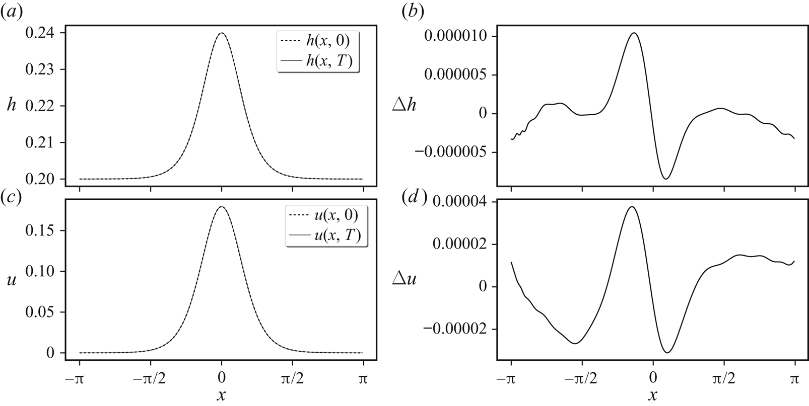
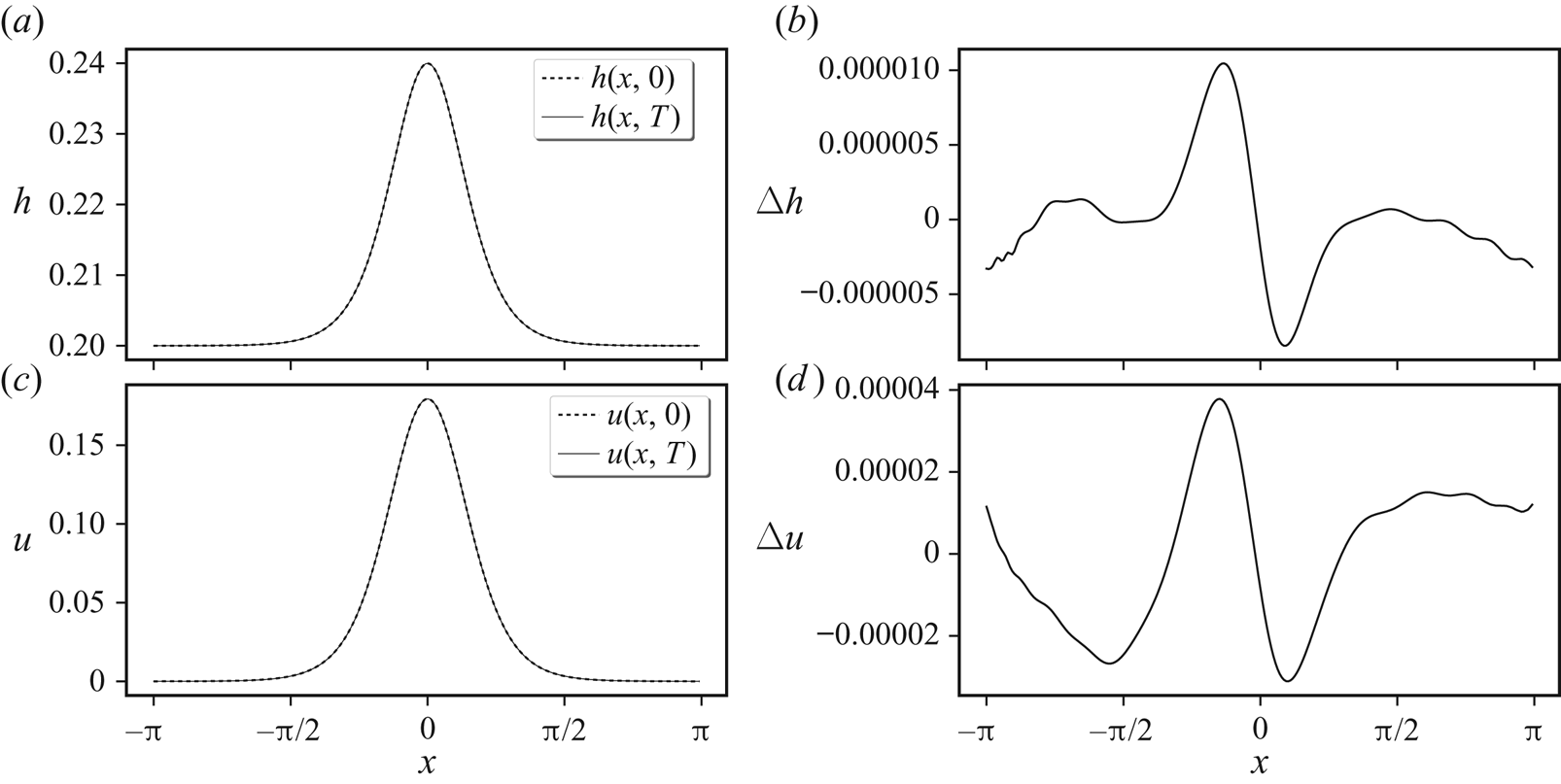
In figure 1, we compare the numerical solution of the reformulated GN model with the above analytical solution after one period of propagation through the ( $x$-periodic) domain,
 $T=2{\rm \pi} /c_0$, taking the domain width equal to
 $2{\rm \pi}$ without loss of generality. Here, we have chosen
 $a=0.04$,
 $h_0=0.2$, and
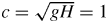 $c=\sqrt {gH}=1$ where
 \[ H=\frac{1}{2{\rm \pi}}\int_{-{\rm \pi}}^{\rm \pi} h\,{\textrm{d}}{x} \]
is the mean fluid depth. This enables one to find  $g$ from
 $c^{2}/H$ and hence
 $c_0=\sqrt {g(h_0+a)}$. For the parameters chosen, we have
 $H\approx 0.207202$ and
 $c_0\approx 1.076238$, giving a period
 $T\approx 5.838100$. The results in the figure show an excellent agreement between the numerical and analytical solution. This verifies (at least without rotation and in one spatial dimension) that the reformulated GN model is mathematically equivalent to the original implicit GN model.
Numerical propagation of a solitary wave for one full period  $T=2{\rm \pi} /c_0$ (the time it takes to pass through the periodic domain).
 $(a,c)$ Dashed lines show the initial (analytical) solutions for
 $h$ and
 $u$, which should be unchanged after one period. The solid lines show the numerical solutions, here using a spatial grid of
 $256$ grid points. Panels
 $(b,d)$ show the differences between the numerical and analytical solutions.
4. Results
In this section, we examine a characteristic example of shear instability at moderate Rossby and Froude numbers, and for a mean height  $H$ equal to the horizontal scale of the initial PV distribution (details are provided below). Simulations have been carried out at two different resolutions, one double the other in each dimension, to verify the results are not sensitive to resolution (in the 2-D models, we also examined resolutions up to eight times finer in
 $x$ and in
 $y$). We begin in § 4.1 with an overview of the numerical methods used, leaving technical details to the appendices. Next, in § 4.2 the initial conditions and flow parameters are specified. Then in § 4.3 we describe the evolution of the 3-D flow, illustrating for the first time the structure of the non-hydrostatic pressure field
 ${{\tilde {P}}}$. Next, in § 4.4 we compare the vertically averaged 3-D fields with the corresponding 2-D fields from the SW and GN simulations, to get a first impression of the improvement afforded by GN over the commonly used SW model. This is then quantified in § 4.5 using error or difference norms, spectra, difference spectra and finally energy differences.
4.1. Numerical methods
The flow domain is doubly periodic horizontally and, in the 3-D simulation, bounded between a flat bottom at  ${{\theta }}=0$ and a free surface at
 ${{\theta }}=H$. For all sets of equations, we employ the same pseudo-spectral method horizontally wherein products are carried out in physical space while derivatives and operator inversions are carried out in spectral space after a fast Fourier transform (FFT). The standard 2/3 de-aliasing rule is used to avoid aliasing errors in all nonlinear products (Fox & Orszag Reference Fox and Orszag1973). In the SW model, only quadratic products occur, but in the other models, higher-order products occur. In such cases, de-aliasing is used repeatedly so that, for example, a cubic product is first decomposed into a quadratic one which is de-aliased after it is calculated, then this quadratic product is multiplied by the remaining field after de-aliasing. Also, the inverse of a field is de-aliased before it is multiplied by another field.
De-aliasing is necessary to prevent the erroneous build up of grid-scale noise which can lead to simulation failure. The numerical algorithms are based directly on those detailed in DJ19, with the only difference being that here we use linearised PV  ${q_l}$ in place of the full Rossby–Ertel PV
 $q$. The latter permits one to use ‘contour advection’ (Dritschel & Ambaum Reference Dritschel and Ambaum1997) to evolve the PV, leading to a more accurate method with significantly less numerical dissipation. However, in the 3-D model, this would lead to a much more complicated algorithm, so it was decided to use the standard pseudo-spectral method instead for all models. For the example studied, the contour advection and pseudo-spectral SW simulations agree closely, with total energy differences
 ${<}1.7\times 10^{-2}\,\%$ at the lowest resolution studied,
 $256^{2}$, and
 ${<}3.3\times 10^{-4}\,\%$ at the higher resolution,
 $512^{2}$.
Time stepping is carried out using an iterated semi-implicit method in which the linear terms in (2.36)–(2.38) (and in the analogous 2-D model equations) are treated implicitly while the nonlinear terms are treated explicitly (see appendix B for details). Iteration is used to improve the estimate of the nonlinear terms at the end of the time step, and the trapezoidal rule is used to average the nonlinear terms over the time step. We use a fixed time step chosen to marginally resolve the highest frequency gravity wave in the SW model (see appendix D in DJ19).
A hyperviscous diffusion operator of the form  $\nu \boldsymbol{\nabla} ^{6}$ is used in all three prognostic equations to absorb the natural nonlinear cascade to small scales which would otherwise build up at the grid scale. We use the same coefficient
 $\nu$ in all three equations, and use the same value previously used in DJ19. For ease of reference, all numerical parameter settings are provided in appendix C.
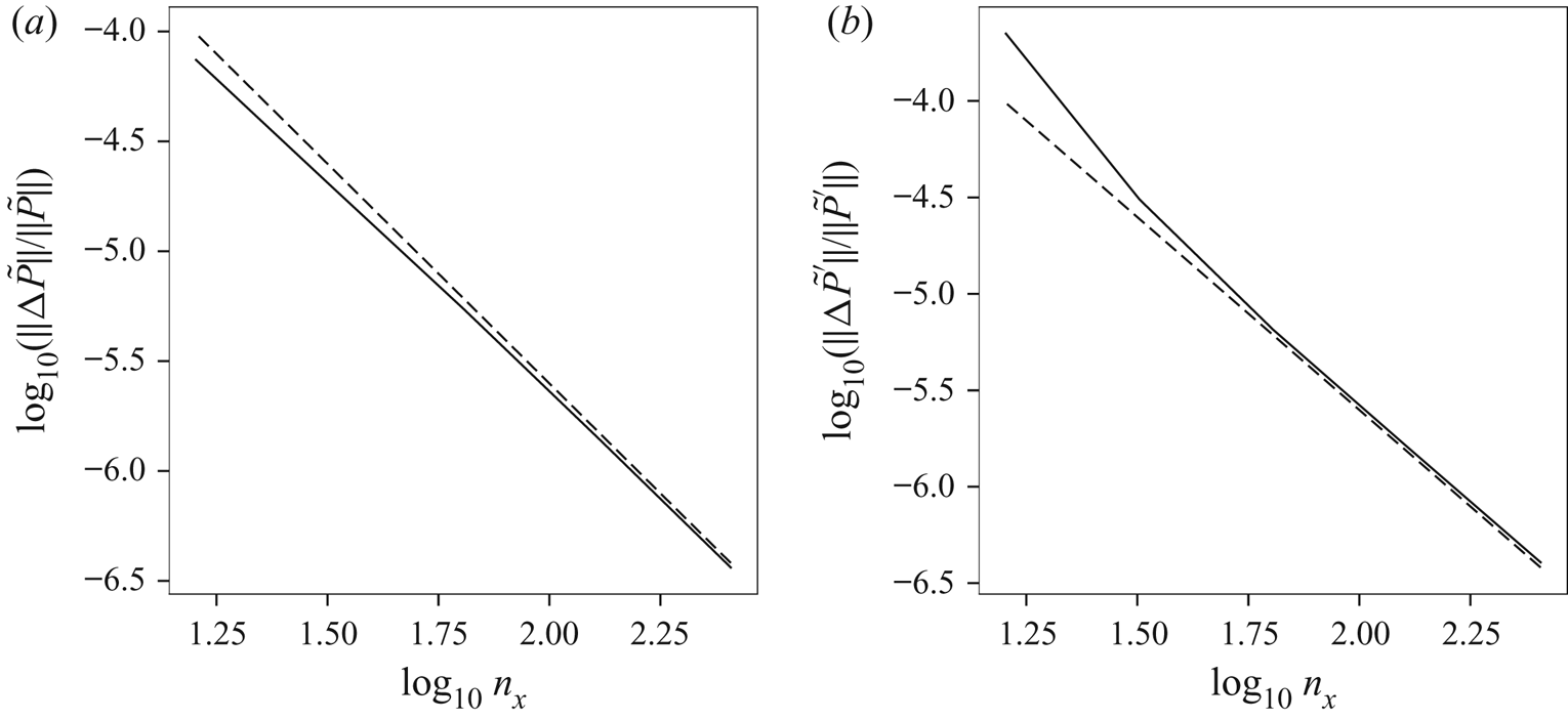
Each method has been tested for accuracy by checking that the numerical results (field norms, energy components, etc.) at early to intermediate times converge with increasing spatial and temporal resolution. Errors scale as the inverse square of the grid resolution, as expected.
4.2. Initial conditions
We examine the same flow studied previously in DJ19 except we consider a mean height  $H$ twice as large, to better test how well the 2-D models capture the vertically averaged 3-D flow. Briefly, the initial flow (having height-independent horizontal velocity
 ${{\boldsymbol {u}}}$) corresponds to a slightly perturbed zonal shear layer, specified in terms of its initial PV in the SW model,
 $q=(\zeta +f)/(1+{{\tilde {h}}})$:
 \begin{equation} q({{\boldsymbol{x}}},0)=\frac{4(y_2(x)-y)(y-y_1(x))}{(y_2(x)-y_1(x))^{2}}f+C, \end{equation}
for  $y_1(x)<y<y_2(x)$, and
 $q=C$ otherwise. Here
 \begin{equation} y_1={-}\frac{1}{2} {\rm \Delta} y \quad\text{and}\quad y_2= \frac{1}{2} {\rm \Delta} y+a_2\sin{2x}+a_3\sin{3x} , \end{equation}
and we have taken  $f=4{\rm \pi}$ for the Coriolis frequency (without loss of generality),
 ${\rm \Delta} y=0.4$ for the width of the shear layer and parameters
 $a_2=0.02$ and
 $a_3=-0.01$ to break the zonal symmetry. We have deliberately chosen
 ${\rm \Delta} y=H$ to ensure that horizontal scales comparable to and smaller than the mean depth are strongly activated. This tests the hydrostatic approximation used in the SW model, and enables us to assess the improvements afforded by the GN model.
The background PV,  $C$, is chosen to ensure that the domain-mean relative vorticity
 $\zeta$ vanishes (required mathematically), using the definition
 $\zeta =(1+{{\tilde {h}}})q-f$. The height anomaly
 ${{\tilde {h}}}$ itself is obtained by ‘balancing’ the initial flow, as in DJ19, which consists of solving the diagnostic equations associated with setting
 ${{\partial }}\delta /{{\partial }}{t}={{\partial }}\gamma _l/{{\partial }}{t}=0$. Balancing helps to reduce the generation of gravity waves initially, allowing one to better study the subsequent spontaneous emission of such waves and the degree to which balance persists (see e.g. Ford, McIntyre & Norton Reference Ford, McIntyre and Norton2000; Mohebalhojeh & Dritschel Reference Mohebalhojeh and Dritschel2001; Norbury & Roulstone Reference Norbury and Roulstone2002a,Reference Norbury and Roulstoneb; Mohebalhojeh & Dritschel Reference Mohebalhojeh and Dritschel2007; Dritschel et al. Reference Dritschel, Gottwald and Oliver2017, and references therein).
Once the initial balanced flow is obtained, the linearised PV anomaly is calculated from  ${q_l}=\zeta -f{{\tilde {h}}}$. The balancing procedure already provides
 $\delta$ and
 $\gamma _l$, and thus
 ${{\boldsymbol {u}}}$ also. These 2-D fields are used to initialise all simulations, including the 3-D one. For the 3-D initialisation, all that is required is to use the 2-D fields
 ${q_l}$,
 $\delta$ and
 $\gamma _l$ on each
 ${{\theta }}$ coordinate surface. In this way, the horizontal velocity
 ${{\boldsymbol {u}}}$ is independent of depth (and equal in all simulations initially), and the dimensionless layer thickness anomaly
 ${{\tilde {\rho }_\theta }}={{\tilde {h}}}$. Note: there is no need to add a 3-D perturbation to the initial flow because the non-hydrostatic pressure
 ${{\tilde {P}}}$, if non-zero, necessarily varies with height due to the boundary conditions required. This means that the horizontal acceleration, involving
 $\boldsymbol {\nabla }{{\tilde {P}}}$, varies with height, and this causes variations in
 ${{\boldsymbol {u}}}$ and in all other 3-D fields to develop in time.
In the SW simulation, the mean depth  $H$ only appears in combination with gravity
 $g$ in the product
 $c^{2}=gH$, a characteristic short-scale squared gravity-wave speed. We specify
 $c$ through the ‘Rossby deformation length’
 $L_D=c/f$, here taken to be
 $0.5$, giving
 $c=2{\rm \pi}$. Rotation tends to suppress free-surface variations at scales
 ${<}L_D$ (see e.g. Vallis Reference Vallis2008). In all other simulations,
 $H$ is required as well, and we take
 $H=0.4$, the same as the width
 ${\rm \Delta} y$ of the initial PV strip in (4.1)–(4.2a,b). At the horizontal resolutions considered (
 $256^{2}$ and
 $512^{2}$), this means that we resolve a wide range of horizontal scales having wavelengths
 ${<}H$, giving ample scope for 3-D motions to develop. To ensure adequate resolution of these motions,
 $32$ uniformly spaced layers in
 ${{\theta }}$ are used for the
 $256^{2}$ simulation, and
 $64$ are used for the
 $512^{2}$ simulation. The vertical grid scale
 ${\rm \Delta} {{\theta }}$ is then very nearly half of the horizontal grid scale
 ${\rm \Delta} x$.
For the parameters chosen, the Rossby number  $Ro=|\zeta |_{\textit{max}}/f$ starts at
 $0.659$ and subsequently varies between
 $0.602$ and
 $0.757$ over the course of the
 $512^{2}$ SW simulation (
 $0\leq t\leq 25$). The Froude number
 $Fr=(\|{{\boldsymbol {u}}}\|/\sqrt {gh})_{\textit{max}}$ starts at
 $0.175$ and subsequently varies between
 $0.175$ and
 $0.235$. The depth anomaly
 ${{\tilde {h}}}$ varies between
 $-0.250$ and
 $0.036$.
4.3. Three-dimensional flow evolution
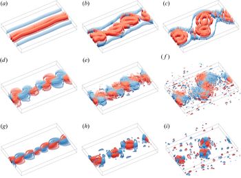
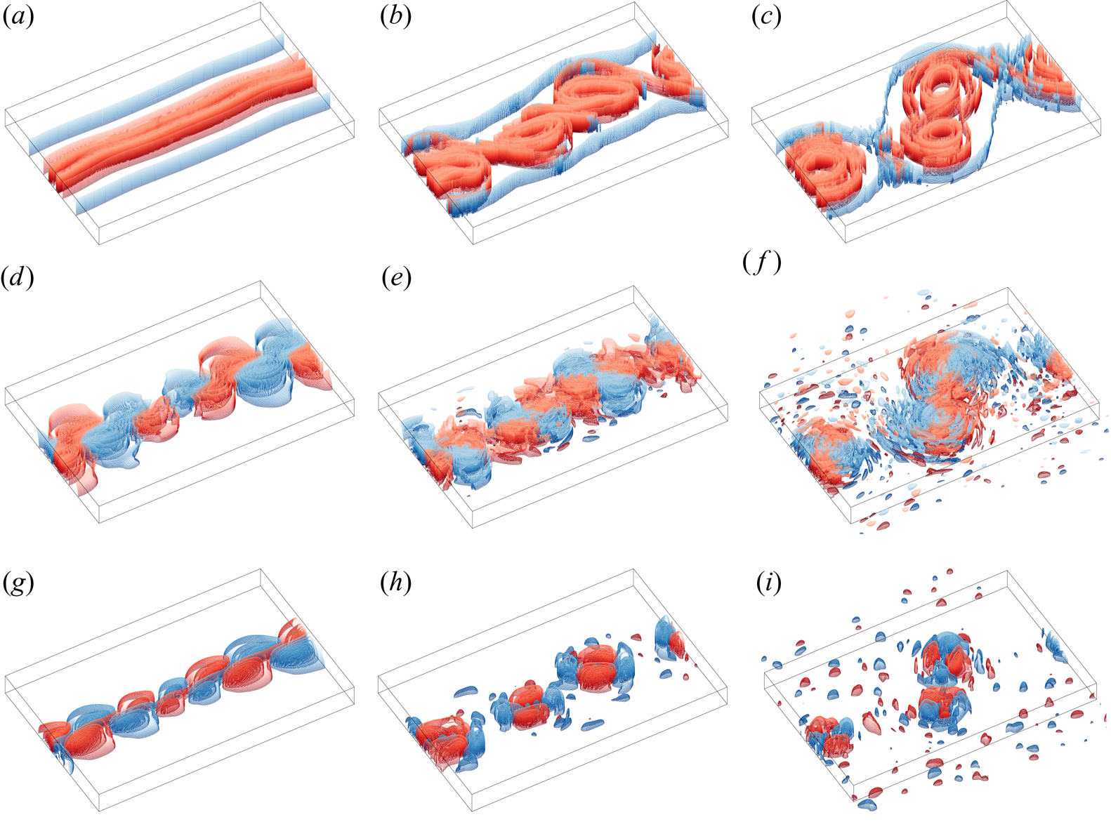
To set the stage, we first examine images of selected fields at early, intermediate and late times from the high-resolution 3-D simulation. Figure 2 shows vertical vorticity  $\zeta$, horizontal divergence
 $\delta$ and non-hydrostatic pressure
 ${{\tilde {P}}}$ at early, intermediate and late times (the final time is
 $t=25$). Note,
 $\zeta$ and
 $\delta$ are calculated in
 ${{\theta }}$ coordinates here. The initial strip of vorticity destabilises and rolls up into a series of vortices which subsequently interact and eject filaments of vorticity. The evolution is qualitatively similar to that observed in 2-D flows (Dritschel Reference Dritschel1989; Waugh & Dritschel Reference Waugh and Dritschel1991), especially for
 $\zeta$ which exhibits only very weak 3-D variations. This is consistent with the assumption made by the 2-D models that the horizontal flow
 ${{\boldsymbol {u}}}$ is height independent. However,
 $\delta$ exhibits much stronger 3-D variations and they grow in time (there are no 3-D variations initially). Hence, the divergent part of
 ${{\boldsymbol {u}}}$ does vary with height, though the contribution of
 $\delta$ to
 ${{\boldsymbol {u}}}$ is here much smaller than that of
 $\zeta$ to
 ${{\boldsymbol {u}}}$. The reason why
 $\delta$ (and to a lesser extent
 $\zeta$) develops 3-D variations is that the non-hydrostatic pressure
 ${{\tilde {P}}}$ is necessarily height dependent, on account of the mixed boundary conditions
 ${{\partial }}{{\tilde {P}}}/{{\partial }}{z}=0$ at
 $z=0$ and
 ${{\tilde {P}}}=0$ at
 $z=h$. This means that
 ${{\tilde {P}}}$ tends to form paraboloidal structures with maximum amplitude on the bottom boundary, as observed in figure 2(
 $g$–
 $i$). As
 $\boldsymbol {\nabla }{{\tilde {P}}}$ contributes to the horizontal acceleration, then vertical variations necessarily develop in
 ${{\boldsymbol {u}}}$ and consequently in
 $\zeta$ and in
 $\delta$. The contribution to
 $\delta$ is much stronger than to
 $\zeta$, since the curl of the non-hydrostatic pressure gradient is much weaker than its divergence. Moreover,
 $\delta$ tends to be significantly weaker than
 $\zeta$ at the Rossby and Froude numbers under consideration, so the relative contribution of
 ${{\tilde {P}}}$ to
 $\delta$ is greater. Notably, in
 $z$ coordinates,
 ${{\tilde {P}}}$ does not contribute directly to the vertical vorticity evolution, since the curl of the pressure gradient vanishes. In summary, divergence is most affected by the 3-D variations induced by the non-hydrostatic pressure.
Vertical vorticity  $\zeta$ (
 $a$–
 $c$), horizontal divergence
 $\delta$ (
 $d$–
 $f$) and non-hydrostatic pressure
 ${{\tilde {P}}}$ (
 $g$–
 $i$) at times
 $t=2$,
 $10$ and
 $25$ (
 $a$–
 $c$,
 $d$–
 $f$ and
 $g$–
 $i$, respectively) in an orthographic perspective, seen from a longitude of
 $30^{\circ }$ and co-latitude of
 $45^{\circ }$, from the high resolution 3-D simulation. The view shows the sub-domain
 $|x| \leq {\rm \pi}$,
 $|y| \leq 2$, and
 $0 \leq \theta \leq H$, with
 $\theta$ stretched by the ‘natural’ scale factor
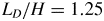 $L_D/H=1.25$ (see Dritschel, de la Torre Juárez & Ambaum Reference Dritschel, de la Torre Juárez and Ambaum1999). Evenly spaced iso-surfaces are rendered red for positive values and blue for negative values, and the colours darken with depth. For a given contour interval
 $\Delta$, surfaces correspond to the field levels
 ${\pm }\Delta /2$,
 ${\pm }3\Delta /2$,…. (
 $a$)–(
 $c$)
 ${\rm \Delta} \zeta =1$, (
 $d$)–(
 $\,f$)
 ${\rm \Delta} \delta =0.02$ except in
 $(d)$ where
 ${\rm \Delta} \delta =0.004$ and (
 $g$)–(
 $i$)
 ${\rm \Delta} {{\tilde {P}}}=0.004$ except in
 $(g)$ where
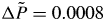 ${\rm \Delta} {{\tilde {P}}}=0.0008$.
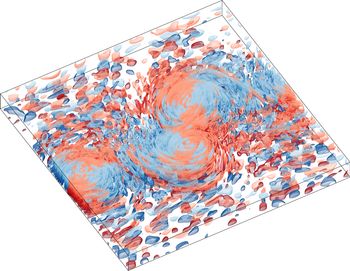
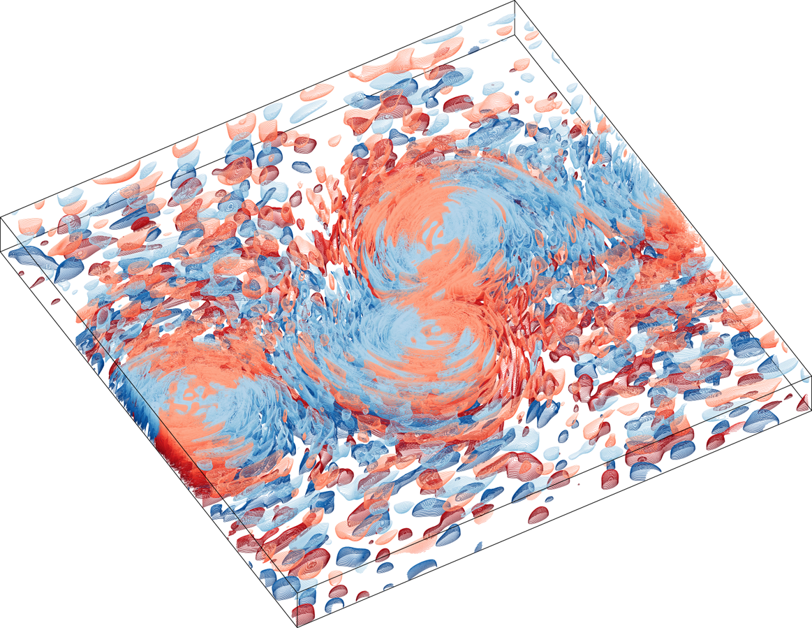
A full-domain view of the divergence at the final time  $t=25$ is shown in figure 3. Here the contour interval is halved to show more of the small-amplitude structures, many of which are confined close to the bottom or to the free surface. The larger-amplitude structures centred on
 $y=0$ have larger scale and extend throughout depth, though it is not readily apparent due to the high degree of complexity. This figure makes it clear, however, that the divergent part of
 ${{\boldsymbol {u}}}$ is not height independent. This violates the primary assumption made when deriving the 2-D models (see § 3), and the implications are examined next in § 4.4.
Divergence field  $\delta$ at
 $t=25$ shown in the same perspective as in figure 2 but over the full domain and with a contour interval twice as small,
 ${\rm \Delta} \delta =0.01$.
4.4. Comparison with the 2-D models
We next focus on the main issue: to what extent do the SW and GN models capture the vertically averaged flow in the parent 3-D model? We first examine raw field differences to gauge how well each 2-D model performs, then compare spectra, analyse difference spectra and finally examine energy differences.
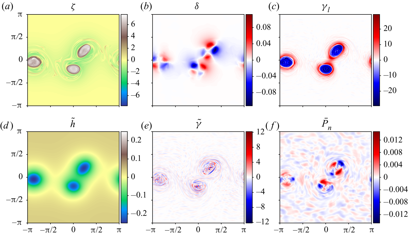
As a point of reference, figure 4 shows, at the final time only, the vertically averaged fields of  $\zeta$,
 $\delta$ and
 $\gamma _l$ (
 $a$–
 $c$) together with the dimensionless height anomaly
 ${{\tilde {h}}}$, the vertically averaged field of
 $\tilde {\gamma }$ and the vertically integrated non-hydrostatic pressure
 $\bar {P}_n$. At this time, the 2-D simulation results generally differ the most, though they closely resemble what is shown in figure 4 apart from the SW results for
 $\bar {P}_n$ (in the SW model
 $\bar {P}_n=0$).
Vertically averaged  $\zeta$,
 $\delta$,
 $\gamma _l$
 $(a$–
 $c)$,
 ${{\tilde {h}}}$, vertically averaged
 $\tilde {\gamma }$ and
 $\bar {P}_n$
 $(d$–
 $f)$, all at
 $t=25$, obtained from the high-resolution 3-D simulation. Different colourmaps are used for
 $\zeta$ and
 ${{\tilde {h}}}$ to better render these fields.
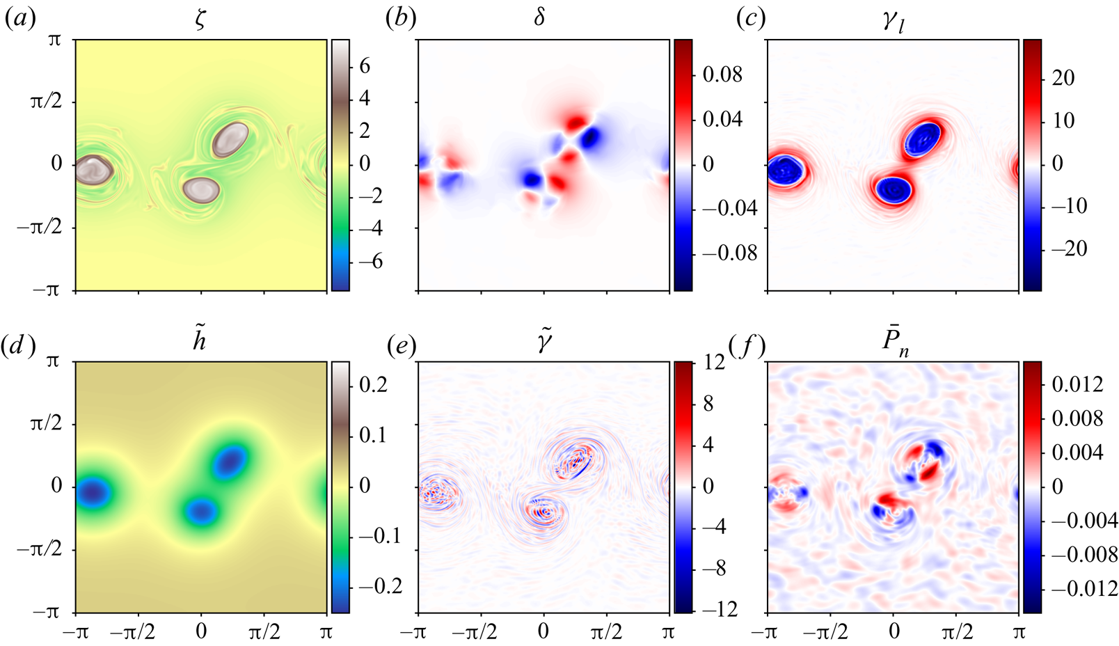
Three prominent vortices are seen in the vorticity field along with weaker vorticity filaments generated earlier when the strip rolled up. The height anomaly field  ${{\tilde {h}}}$ looks like a smoothed version of
 $\zeta$, and indeed under geostrophic balance
 ${{\tilde {h}}}\propto \boldsymbol{\nabla} ^{-2}\zeta$. Geostrophic balance assumes
 $\gamma _l=f\zeta -c^{2}\boldsymbol{\nabla} ^{2}{{\tilde {h}}}=0$. Clearly,
 $\gamma _l$ is not zero here, but nonetheless this balance explains much of the observed structure of
 ${{\tilde {h}}}$. An extended form of geostrophic balance called ‘Bolin–Charney’ balance (Bolin Reference Bolin1955; Charney Reference Charney1955) is obtained by setting
 $\delta =0$ and
 $f\zeta -c^{2}\boldsymbol{\nabla} ^{2}{{\tilde {h}}}+2J_{xy}(u,v)=0$, i.e.
 $\tilde {\gamma }=0$ when
 $\delta =0$, see (3.12) (see also appendix D in Mohebalhojeh & Dritschel Reference Mohebalhojeh and Dritschel2001). Essentially, Bolin–Charney balance includes the flow curvature through
 $J_{xy}(u,v)$. From figure 4, this balance is much closer to being realised than geostrophic balance: not only is the maximum value of
 $|\tilde {\gamma }|$ nearly
 $2.5$ times smaller than that of
 $|\gamma _l|$, the pattern exhibited by
 $\tilde {\gamma }$ is entirely different. It is much smaller scale and less organised, and moreover the root-mean-square (r.m.s.) value of
 $\tilde {\gamma }$ is more than
 $7$ times smaller than that of
 $\gamma _l$. At half-resolution (not shown), the maximum is
 $6$ times smaller and the r.m.s. is
 $16$ times smaller, indicating that
 $\tilde {\gamma }$ is predominantly a small-scale field (as has been verified by considering its power spectrum).
The horizontal divergence field  $\delta$ exhibits multi-polar patterns around the three vortices, evidence of a higher-order balance in the flow (e.g. the balance resulting from setting
 ${{\partial }}\delta /{{\partial }}{t}={{\partial }}\gamma _l/{{\partial }}{t}=0$; see DJ19 who discuss this in relation to the 2-D models). The patterns seen here are not gravity waves; these imbalanced motions are an order of magnitude smaller in amplitude (not shown but see DJ19).
Finally, the pattern seen in the vertically integrated non-hydrostatic pressure  $\bar {P}_n$ is consistent with its diagnostic relation (3.14). Roughly speaking,
 $\bar {P}_n$ resembles that pattern obtained by inverting Laplace's operator on
 $\tilde {\gamma }$. Note that
 $\bar {P}_n$ is broader in scale and tends to have the opposite sign to
 $\tilde {\gamma }$ at extrema.
We turn next to the difference fields obtained by subtracting the above fields from those predicted by the SW and GN models. We concentrate on the representative set of variables  $\zeta$,
 $\delta$,
 ${{\tilde {h}}}$ and
 $\bar {P}_n$ for brevity. As
 $\bar {P}_n=0$ in the SW model, we start by comparing
 $\zeta$,
 $\delta$ and
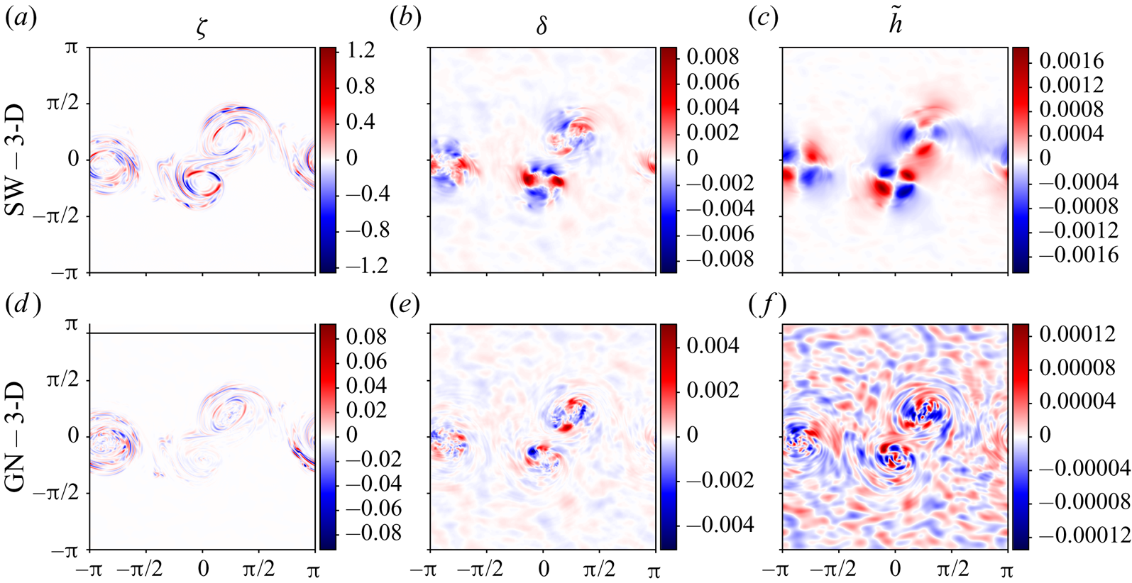
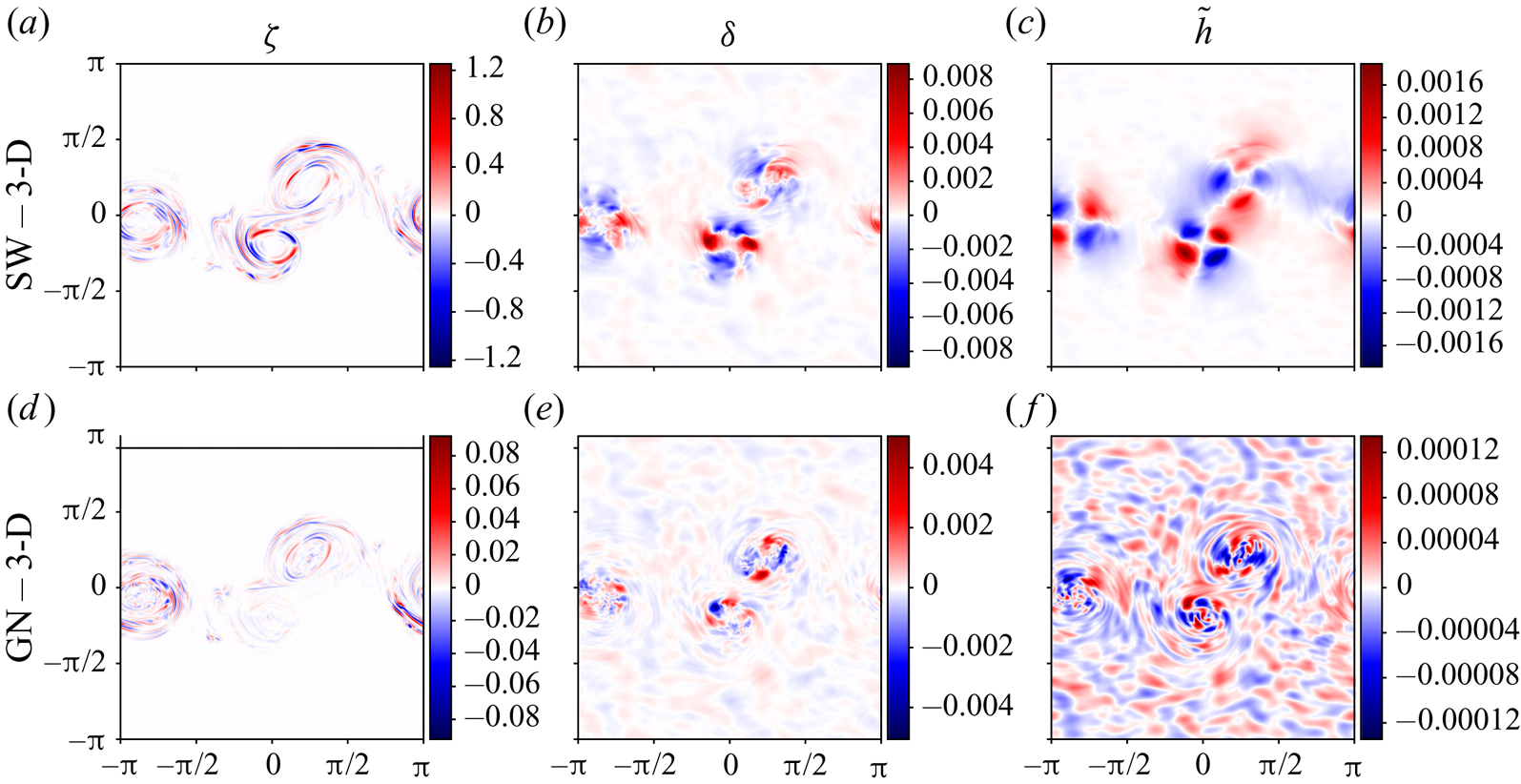
 ${{\tilde {h}}}$ in figure 5. First of all, maximum differences are small in both 2-D models,
 ${<}16.3\,\%$ for
 $\zeta$,
 ${<}8.0\,\%$ for
 $\delta$ and
 ${<}0.75\,\%$ for
 ${{\tilde {h}}}$, with the largest differences consistently found for the SW model. At half-resolution (not shown), these differences reduce to
 $8.3\,\%$ for
 $\zeta$ and
 $5.5\,\%$ for
 $\delta$, but increase slightly to
 $0.76\,\%$ for
 ${{\tilde {h}}}$. This shows that the differences in
 $\zeta$ and
 $\delta$ are predominantly at small scales, which become more important at higher resolution (this is confirmed by examining power spectra in § 4.5). For
 $\delta$, the GN model offers the least improvement over the SW one, reducing maximum differences by approximately a factor of 2, to
 $4.5\,\%$ (or
 $3.2\,\%$ at half-resolution).
Field differences at  $t=25$ between the
 $512^{2}$ SW and GN simulations, and the corresponding 3-D simulation (
 $a,d$,
 $b,e$, and
 $c,f$, respectively). (
 $a,d$) Show the vertically averaged vertical vorticity
 $\zeta$, (
 $b,e$) show the vertically averaged horizontal divergence
 $\delta$ and (
 $c,f$) show the dimensionless height anomaly
 ${{\tilde {h}}}$.
For  $\zeta$ and
 ${{\tilde {h}}}$, the GN model offers substantial improvements over SW. Maximum differences in
 $\zeta$ are
 $13.6$ times smaller in GN relative to SW. The differences in GN are
 ${<}1.2\,\%$, somewhat surprising given the length and complexity of the flow evolution. This error reduces to just
 $0.04\,\%$ at half-resolution, due to the weaker activity at small scales (small positioning errors at high resolution, i.e. the location of sharp vorticity gradients along the edges of the vortices, can lead to significant maximum and r.m.s. differences). For
 ${{\tilde {h}}}$, maximum differences in the GN model are just
 $0.054\,\%$ at the higher resolution, and
 $0.039\,\%$ at the lower resolution.
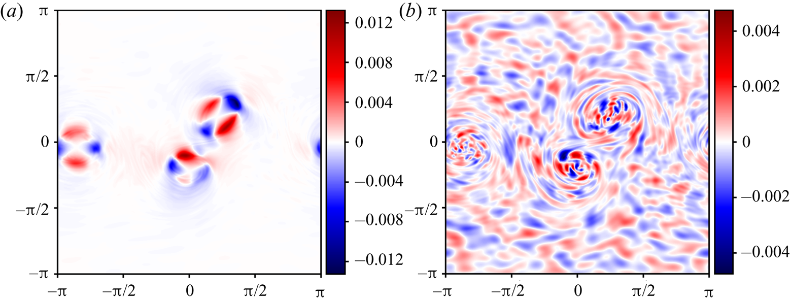
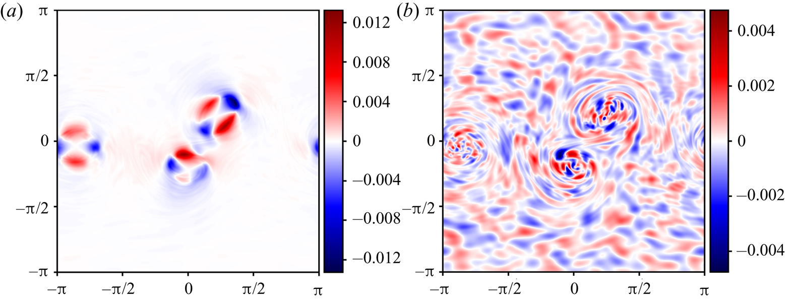
Regarding the non-hydrostatic pressure (which is neglected in the SW model), its vertically integrated form  $\bar {P}_n$ is examined in figure 6 at the final time (
 $t=25$). Here, we show the GN field in (
 $a$), and its difference from the 3-D field in (
 $b$). Notably, maximum differences are approximately
 $32.3\,\%$, and are found primarily in the vortex cores (these reduce to
 $23.4\,\%$ at half-resolution). However, there are differences throughout the domain arising from the fact that
 $\bar {P}_n$ in the 3-D simulation (see figure 4) exhibits significant variations outside the vortex cores, unlike in the GN simulation. These variations are higher-order effects not captured by the GN model, and likely relate to the assumption that the horizontal velocity field
 ${{\boldsymbol {u}}}$ is independent of depth. This is discussed further at the end of this section. Nonetheless, the ability of the GN model to capture a major portion of the true
 $\bar {P}_n$ must account for this model's substantial gain in accuracy over the SW model. After all, the reformulated explicit GN model makes it clear that the only difference from the SW model is the inclusion of
 $\bar {P}_n$.
Vertically integrated non-hydrostatic pressure  $\bar {P}_n$ at
 $t=25$ in the GN simulation
 $(a)$, and the difference between the GN and 3-D simulations
 $(b)$. For reference, see figure 4(
 $\,f$) for
 $\bar {P}_n$ in the 3-D simulation.
4.5. Quantification of error
We next quantify the differences between the 2-D and 3-D simulations by examining relative r.m.s. errors, spectra, difference spectra and energy differences.
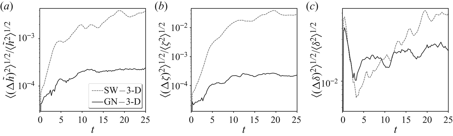
The relative r.m.s. errors of  ${{\tilde {h}}}$,
 $\zeta$ and
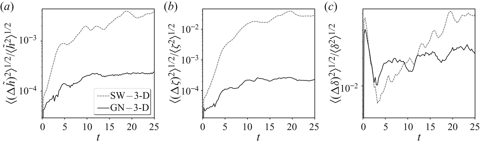
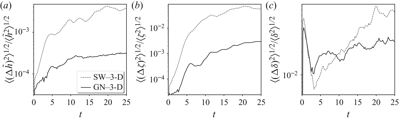
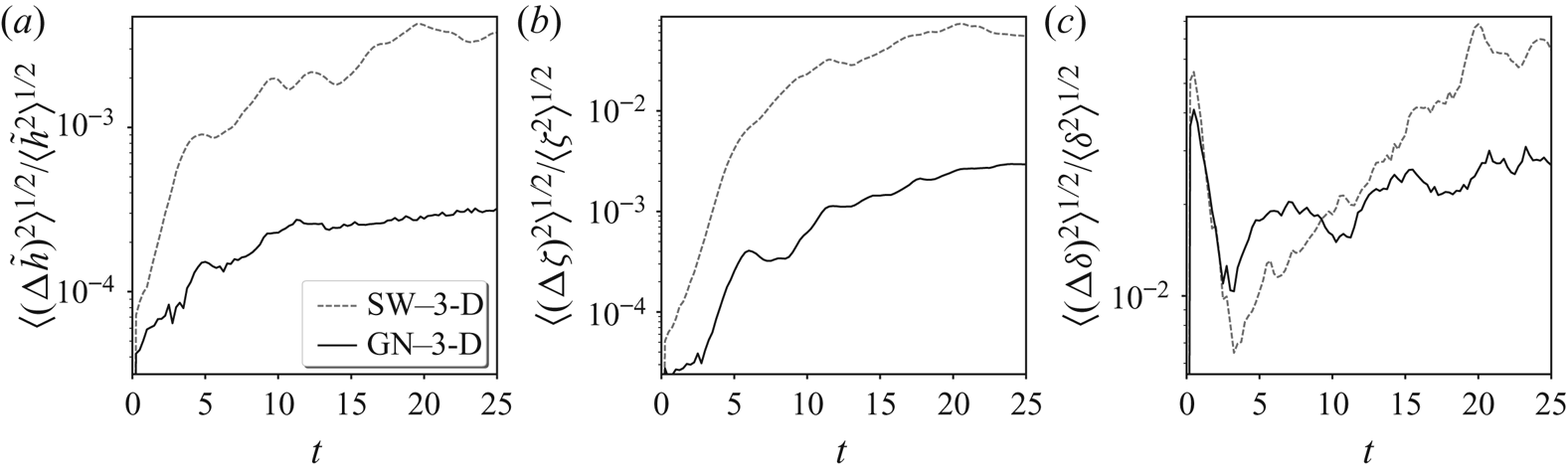
 $\delta$ versus time are shown in figure 7 at the lower resolution, and in figure 8 at the higher resolution. For
 ${{\tilde {h}}}$ and
 $\zeta$, the GN simulation exhibits much lower error than the SW simulation, while for
 $\delta$ the errors are comparable, albeit lowest in the GN simulation. The gain in accuracy of GN over SW is less striking at higher resolution due to the fact that errors predominantly arise at small scales (see power spectra below), and these small scales are more active at higher resolution.
Time evolution, for the lower-resolution simulations, of the relative r.m.s. errors of the dimensionless height anomaly  ${{\tilde {h}}}$, the vertically averaged vertical vorticity
 $\zeta$ and the vertically averaged horizontal divergence
 $\delta$, for the SW and GN simulations, as labelled. The errors are computed from the r.m.s. field differences divided by the r.m.s. three-dimensional field (after vertical averaging). Note the
 $\log _{10}$ scale.
As in figure 7 but for the higher-resolution simulations.
To see how the error is distributed across scale, it is instructive to examine field power spectra. For a given field, say  $\xi$, its spectrum
 $S_\xi (k)$ is computed in the standard way by Fourier transforming
 $\xi$, squaring the spectral amplitudes
 $\hat {\xi }$ for each wavevector
 $(k_x,k_y)$, then summing these squared amplitudes for all wavevectors whose magnitude
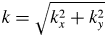 $k=\sqrt {k_x^{2}+k_y^{2}}$ lies in the shell
 $k-1/2<k\leq k+1/2$. Finally,
 $S_\xi (k)$ is multiplied by
 $2/n_x$, where
 $n_x$ is the grid resolution in
 $x$ and in
 $y$ (here
 $512$ at the higher resolution), to be able to compare different resolutions. Uneven sampling of shells is accounted for by further multiplying
 $S_\xi (k)$ by the factor
 $2{\rm \pi} k/N(k)$, where
 $N(k)$ is the number of wavevectors lying in each shell.
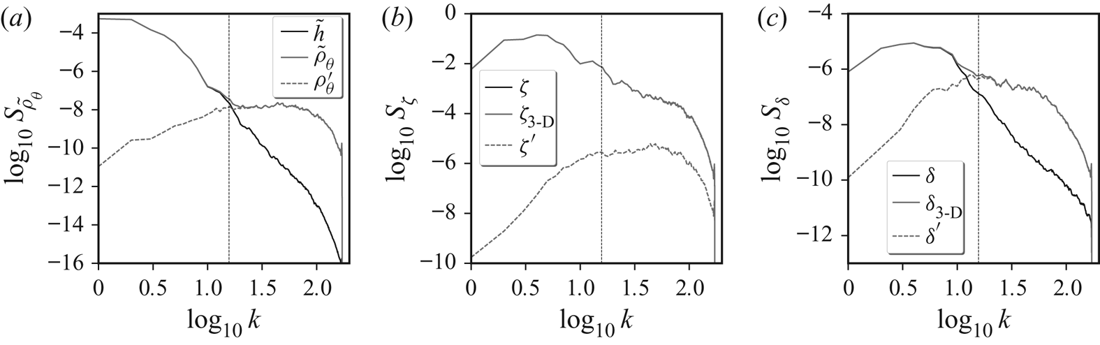
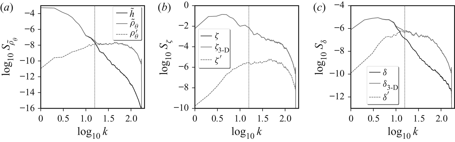
Selected field spectra in the high-resolution 3-D simulation are shown in figure 9 (broadly similar results are found at lower resolution). The spectra are computed three ways. One is to first average each field (over  ${{\theta }}$), then compute the spectrum from this averaged field (dark solid lines in the figure). The next is to compute the spectrum of a field in each layer, then average the spectrum (light solid lines). In this case, 3-D variations are included. Finally, the spectrum is also computed from the departure of each field from its
 ${{\theta }}$ average (dashed lines). This decomposition shows that 3-D variations are most pronounced at small scales, i.e. for wavelengths comparable to or smaller than
 $H$ (or for wavenumbers
 $k > 2{\rm \pi} /H$, marked as a vertical reference line in each panel of the figure). For
 $\zeta$, the 3-D variations contribute negligibly, but for
 ${{\tilde {\rho }_\theta }}$ and
 $\delta$ they dominate for
 $k > 2{\rm \pi} /H$. Hence, the 3-D variations seen in
 $\delta$ in figure 3 are confined to small scales; at large scales
 $\delta$ is in fact predominantly 2-D.
Power spectra of  ${{\tilde {\rho }_\theta }}$,
 $\zeta$ and
 $\delta$ (
 $a$–
 $c$) in the high-resolution 3-D simulation at
 $t=25$. The spectra of the vertically averaged fields are shown in dark solid lines (labelled
 $\tilde {h}$,
 $\zeta$ and
 $\delta$). Note:
 ${{\tilde {h}}}$ is the vertical average of
 ${{\tilde {\rho }_\theta }}$. The vertically averaged spectra of the fields in each layer are shown in light solid lines (labelled
 ${{\tilde {\rho }_\theta }}$,
 $\zeta _{\textrm {3-D}}$ and
 $\delta _{\textrm {3-D}}$). These are the uppermost curves in each panel. Finally, the vertically averaged spectra of the difference fields (removing the vertical average) in each layer are shown in light dashed lines (labelled
 ${{\tilde {\rho }_\theta }}'$,
 $\zeta '$ and
 $\delta '$). The dashed vertical line marks the transition wavenumber
 $k=2{\rm \pi} /H$, where
 $H$ is the mean height.
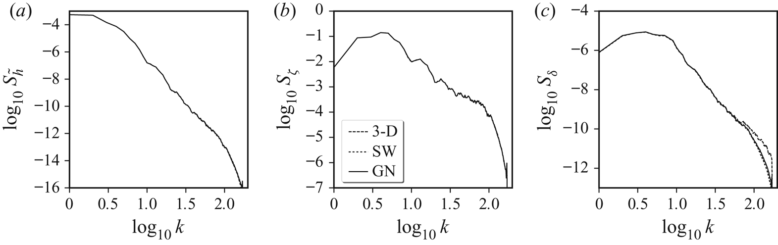
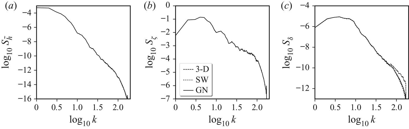
We return next to comparing the SW and GN simulations with the 3-D one. Figure 10 compares  ${{\tilde {h}}}$,
 $\zeta$ and
 $\delta$ spectra between the high-resolution simulations at the final time. Note: spectra in the 3-D simulation are computed from the
 ${{\theta }}$-averaged fields. Overall, the agreement is excellent, in particular for
 ${{\tilde {h}}}$ and
 $\zeta$, for which all curves lie on top of one another (see below for a quantification of the differences). For
 $\delta$, however, differences appear predominantly at high wavenumbers
 $k$. There, the 3-D spectrum has several times more power than either the SW or the GN spectra, both of which are close to one another. At higher resolutions (up to at least
 $2048^{2}$), the SW and GN spectra continue to show a comparably steep slope at high wavenumbers.
Comparison of various spectra at  $t=25$ obtained from the high-resolution 3-D simulation (after a
 ${{\theta }}$ average), and the corresponding SW and GN simulations (as labelled). Spectra are shown for
 ${{\tilde {h}}}$,
 $\zeta$ and
 $\delta$ (
 $a$–
 $c$). Differences are only evident in the
 $\delta$ spectra at high
 $k$ (see below for difference spectra).
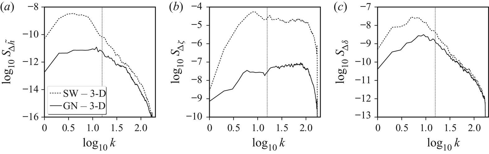
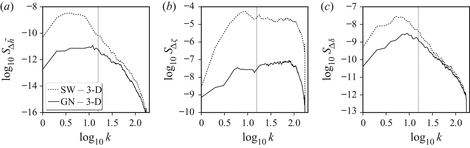
Spectra for various difference fields are shown in figure 11. For a given field  $\xi$ in either the SW or GN simulation, we first subtract the corresponding
 ${{\theta }}$-averaged field in the 3-D simulation to form
 ${\rm \Delta} \xi$, then compute its spectrum. The results in this figure underscore the large improvement the GN model makes over the SW model. Thus, including non-hydrostatic pressure allows one to much better approximate the vertically averaged 3-D flow. Notably, this is true across all scales, with the biggest improvement found for vorticity
 $\zeta$, i.e. for the non-divergent motions. On the other hand, there is only a modest improvement for height
 ${{\tilde {h}}}$ and divergence
 $\delta$ at scales smaller than the mean depth, i.e.
 $k>2{\rm \pi} /H$. Fundamentally, this is due to the 3-D nature of the non-hydrostatic pressure, which impacts both divergence and height (see e.g. figure 3). Similar results are found at lower resolution, albeit with the GN model exhibiting a more substantial gain in accuracy over the SW model (not shown).
Difference spectra at  $t=25$ for
 ${{\tilde {h}}}$,
 $\zeta$ and
 $\delta$ (
 $a$–
 $c$) computed from the differences between the SW and GN fields, and the corresponding
 ${{\theta }}$-averaged 3-D field (as labelled). The dashed vertical line marks the transition wavenumber
 $k=2{\rm \pi} /H$.
Finally, we consider how well the various simulations compare energetically. The time evolution of the kinetic  $\mathcal {K}$, potential
 $\mathcal {P}$ and total
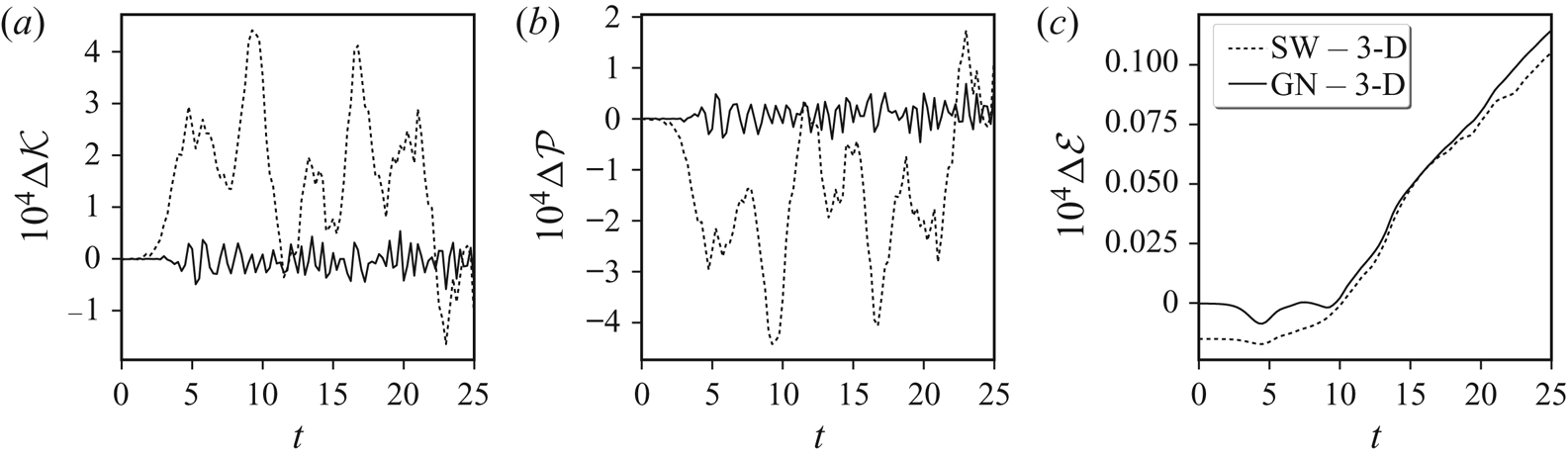
 $\mathcal {E}=\mathcal {K}+\mathcal {P}$ energy differences (SW-3D and GN-3D) are examined in figure 12. Over the time period considered,
 $\mathcal {K}$ varies from
 $1.897$ to
 $1.977$,
 $\mathcal {P}$ varies from
 $2.180$ to
 $2.260$, while
 $\mathcal {E}$ decreases from
 $4.157$ to
 $4.156$ (to three decimal places). The energy differences seen in figure 12 are much smaller than these energy variations. The GN-3D
 $\mathcal {K}$ and
 $\mathcal {P}$ differences, for example, are
 ${<}0.05\,\%$ of the ranges in
 $\mathcal {K}$ and
 $\mathcal {P}$. Furthermore, the GN-3D
 $\mathcal {E}$ differences are
 ${<}1\,\%$ of the total decrease in
 $\mathcal {E}$ found in the 3-D simulation. At half-resolution, these differences are even smaller:
 $0.04\,\%$ for
 $\mathcal {K}$ and
 $\mathcal {P}$ and
 $0.6\,\%$ for
 $\mathcal {E}$.
Differences in kinetic, potential and total energies ( $a$–
 $c$) between the higher resolution SW and GN simulations, and the corresponding 3-D simulation (as labelled). Note that the energy differences are multiplied by
 $10^{4}$. For reference, the time mean kinetic, potential and total energies in the 3-D simulation are
 $1.922$,
 $2.235$ and
 $4.157$ (to three decimal places).

The SW-3D differences are substantially larger for both  $\mathcal {K}$ and
 $\mathcal {P}$, and do not vary significantly with resolution (not shown). Note that the initial difference in
 $\mathcal {E}$ between the SW and 3-D simulations arises from the fact that the SW model neglects the vertical velocity contribution to
 $\mathcal {K}$, see (3.18).
In every measure considered, the GN model provides a significantly better approximation to the vertically averaged 3-D flow than the SW model. The (reformulated, explicit) GN model moreover exhibits the same regularity, i.e. the same spectral decay at high wavenumbers  $k\gg 2{\rm \pi} /H$, as the 3-D model (for the vertically averaged fields). The SW model also exhibits comparable regularity. Both the GN and SW models are robust at resolutions at least four times higher in
 $x$ and in
 $y$, retaining the numerical parameter settings set out in appendix C.
Why does the GN model perform so well? As already pointed out, the specific flow examined here starts with horizontal scales equal to the mean fluid height  $H$, and moreover uses a Rossby deformation length
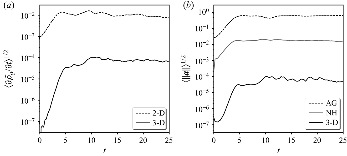
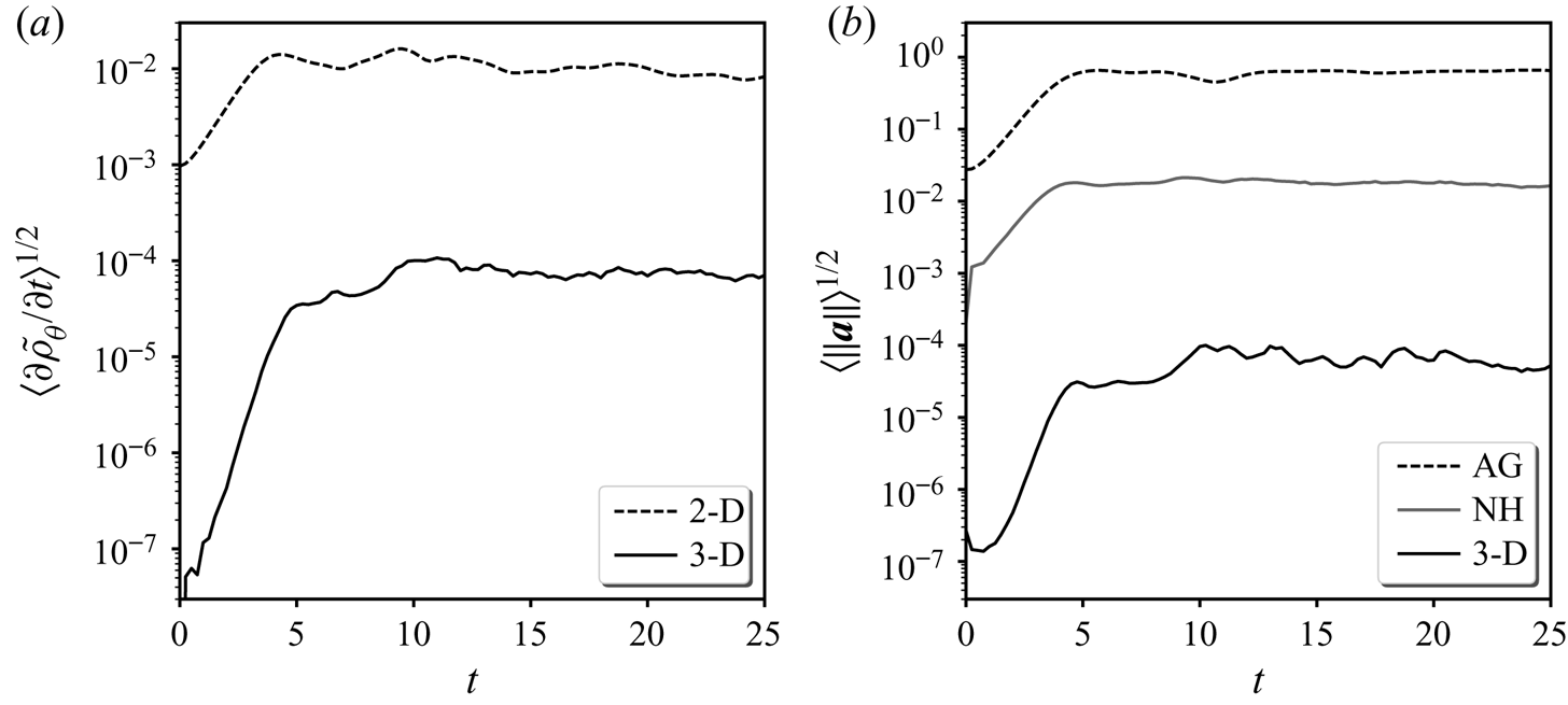
 $L_D \sim H$. We have seen that certain components of the 3-D flow do have significant vertical variations, yet the vertically averaged flow is nonetheless well captured by the GN model, in particular. To help understand this, we next probe the 3-D flow to estimate the contribution of vertical variations to the vertically averaged flow. Figure 13 shows the changes in mass
 ${{\partial }}{{\tilde {\rho }_\theta }}/{{\partial }}{t}$ and the acceleration
 ${{\boldsymbol {a}}}={\textrm {D}}{{\boldsymbol {u}}}/{\textrm {D}}{t}$ broken down into various contributions. Denoting
 ${{\boldsymbol {u}}}_0$ as the vertically averaged horizontal flow, in
 ${{\partial }}{{\tilde {\rho }_\theta }}/{{\partial }}{t}$ (
 $a$) we show both the r.m.s. value of the 2-D contribution
 $-\boldsymbol {\nabla }\boldsymbol {\cdot }((1+{{\tilde {h}}}){{\boldsymbol {u}}}_0)$ and the remaining, 3-D contribution versus time. The latter is more than
 $120$ times smaller (
 $500$ times smaller at the lower resolution), so at most plays a very minor role.
Local changes in mass  ${{\partial }}{{\tilde {\rho }_\theta }}/{{\partial }}{t}$ (
 $a$) and in acceleration
 ${{\boldsymbol {a}}}$ (
 $b$) broken down into various contributions (as labelled). In
 ${{\partial }}{{\tilde {\rho }_\theta }}/{{\partial }}{t}$, ‘2-D’ refers to the contribution from the vertically averaged flow, while ‘3-D’ refers to the remainder. In
 ${{\boldsymbol {a}}}$, ‘AG’ refers to the ageostrophic acceleration (see text for definition), ‘NH’ refers to the non-hydrostatic contribution, while ‘3-D’ refers to the vertically varying part of
 $-{{\boldsymbol {u}}}\boldsymbol {\cdot }\boldsymbol {\nabla }{{\boldsymbol {u}}}$.
Regarding the acceleration, we examine three contributions. The first is the ‘ageostrophic’ acceleration  ${{\boldsymbol {a}}}_{AG}=-f{{\boldsymbol {k}}}\times {{\boldsymbol {u}}}-g\boldsymbol {\nabla }{h}$, which is small when the flow Rossby number
 $Ro$ is small (here
 $Ro\approx 0.7$). The next is the non-hydrostatic acceleration,
 ${{\boldsymbol {a}}}_{NH}=-\boldsymbol {\nabla }{{\tilde {P}}}$ (in
 $z$ coordinates), and the third is the ‘3-D’ acceleration
 ${{\boldsymbol {a}}}_{\textrm {3D}}={{\boldsymbol {u}}}_0\boldsymbol {\cdot }\boldsymbol {\nabla }{{\boldsymbol {u}}}_0-{{\boldsymbol {u}}}\boldsymbol {\cdot }\boldsymbol {\nabla }{{\boldsymbol {u}}}$, equal to the vertically varying part of
 $-{{\boldsymbol {u}}}\boldsymbol {\cdot }\boldsymbol {\nabla }{{\boldsymbol {u}}}$. Again, the contribution of
 ${{\boldsymbol {a}}}_{\textrm {3D}}$ is more than
 $300$ times smaller than
 ${{\boldsymbol {a}}}_{NH}$, which in turn is more than
 $40$ times smaller than
 ${{\boldsymbol {a}}}_{AG}$ (these ratios are
 $1000$ and
 $50$, respectively, for the lower-resolution simulations). While both
 ${{\boldsymbol {a}}}_{NH}$ and
 ${{\boldsymbol {a}}}_{AG}$ are calculated from the full 3-D flow, they are likely to be dominated by the vertically averaged 2-D flow. The conclusion is that 3-D variations play very minor roles in the flow regime studied.
Regarding numerical cost, the simulations were all performed on the same workstation, on a serial processor (Intel i7-8700) in double precision. At  $512^{2}$ resolution, the SW and GN models required 5401 and 19,055 s of CPU time, respectively (the implicit GN model used in DJ19 required 47 500 s). The extra cost of the (explicit) GN model is partly associated with the iteration required to find the vertically integrated non-hydrostatic pressure
 $\bar {P}_n$ from (3.14), and partly associated with the evaluation of additional nonlinear terms in (3.15)–(3.17). Whether this extra cost is worth it depends on the question being asked: if one wants to understand the role of non-hydrostatic effects in fundamental problems like balance and the spontaneous emission of gravity waves (where the GN and SW dispersion relations differ significantly, see e.g. DJ19), then GN is necessary and is certainly more cost effective than running a full 3-D simulation, which, at
 $512\times 512\times 64$ resolution, required
 $3.95\times 10^{6}\ \textrm {s}$ of CPU time. In this case, the GN simulation is
 $200$ times more efficient. Moreover, the excellent agreement between the GN and 3-D results demonstrates we can learn much from this new model.
5. Conclusions
We have compared the traditional two-dimensional hydrostatic shallow-water model and its non-hydrostatic extension with their parent three-dimensional model (Euler's equations) in the context of a rotating, homogeneous layer of fluid having a free upper surface. We have focussed on a flow regime characteristic of a wide range of motions occurring in the Earth's atmosphere and oceans, namely when the Rossby and Froude numbers are both smaller than unity (see e.g. Vallis Reference Vallis2008, and references). In an example of shear instability, the roll up of a strip of potential vorticity (arguably a generic process in geophysical flows), we have examined how well these two-dimensional models capture the vertically averaged flow in the three-dimensional model, even when the typical horizontal scale of the flow is comparable with the mean fluid depth  $H$. Under these circumstances, one would expect the long-wave assumption underpinning both two-dimensional models to be invalid, particularly for the shallow-water model. Surprisingly, this model nevertheless captures a large fraction of the actual vertically averaged flow.
The non-hydrostatic two-dimensional model, the Serre/Green–Naghdi model – here explicitly re-formulated to use non-hydrostatic pressure – does significantly better. Whereas, in the high-resolution example considered, maximum errors in vorticity may reach nearly  $16.3\,\%$ in the shallow-water model, they are reduced to
 $1.2\,\%$ in the GN model. This is a substantial error reduction. Maximum errors in the free-surface height anomaly are much smaller:
 $0.75\,\%$ in the SW model reducing to just
 $0.054\,\%$ in the GN model. However, results for the horizontal divergence are not nearly as impressive: only moderate error reductions are achieved, from
 $8.0\,\%$ to
 $4.5\,\%$. This is because the horizontal divergence in the parent three-dimensional model exhibits significant 3-D variations, inherited from non-hydrostatic pressure, particularly at horizontal scales of order
 $H$ or less. Thus, the fundamental assumption in the two-dimensional models that the horizontal flow is independent of depth does not hold for the divergent part of the flow at these scales.
The GN model employed here is a mathematically reformulated, explicit version of the original, implicit GN model (Ertekin Reference Ertekin1984; Demirbilek & Webster Reference Demirbilek, Webster and Herbich1999; Pearce & Esler Reference Pearce and Esler2010; Dritschel & Jalali Reference Dritschel and Jalali2019). However, for numerical simulation, the explicit GN model is not only much more efficient but also more robust and accurate. The explicit GN model diagnoses the vertically integrated non-hydrostatic pressure  $\bar {P}_n$ from a simple, linear, robustly convergent elliptical equation. This equation is found from combining two results. The first comes from vertically integrating the vertical momentum equation, using the fact that the vertical velocity must be a linear function of
 $z$ on account of 3-D incompressibility. In this way, the non-hydrostatic pressure is found to be a quadratic function of
 $z$. Integrating gives
 $\bar {P}_n$. The second result comes from taking the horizontal divergence of the horizontal momentum equations. Between these two results, one can eliminate the time derivatives, leading to the elliptic equation for
 $\bar {P}_n$.
The approach taken to derive the explicit GN model may be extended in a variety of ways. For example, one can apply it to derive multi-layer shallow-water formulations – now including non-hydrostatic effects. The recipe is simple: first obtain an expression for the vertically integrated non-hydrostatic pressure over each layer, making use of the vertical momentum equation and the fact that the vertical velocity is a linear function of  $z$ in each layer. Next, take the horizontal divergence of the horizontal momentum equations. Combining these results gives diagnostic equations for the pressures, albeit coupled now from layer to layer. Nonetheless, they are linear elliptic equations, and may be readily solved numerically. This approach differs fundamentally from that taken to derive higher-level GN models (see Shields & Webster Reference Shields and Webster1988; Demirbilek & Webster Reference Demirbilek, Webster and Herbich1999), and moreover remains explicit for any number of layers. Another advantage is that the layers can differ in density; one must only assume the density is uniform in each layer. A two-layer model is under development and we hope to report on this and the generalisation to many layers in a future paper.
Acknowledgements
D.G.D. would like to thank E.R. Johnson for his helpful comments on the research underpinning this study. Support for this research has come from the UK Engineering and Physical Sciences Research Council (grant no. EP/H001794/1).
Declaration of interests
The authors report no conflict of interest.
Appendix A. The pressure solver
The numerical solution procedure for the non-hydrostatic pressure  ${{\tilde {P}}}$ in (2.27) was tested using analytical forms for
 ${{\rho _\theta }}$ and
 ${{\tilde {P}}}$, from which one can compute all terms involving
 ${{\tilde {P}}}$ in (2.27) explicitly. The ‘source’ term
 $S_0$, which is independent of
 ${{\tilde {P}}}$, is calculated as the residue in this equation, i.e.
 \begin{equation} S_0=\boldsymbol{\nabla}^{2}{{\tilde{P}}}+\frac{\partial^{2}{{{\tilde{P}}}}}{\partial{{{\theta}}}^{2}} -{{\boldsymbol{\sigma}}}\boldsymbol{\cdot}\boldsymbol{\nabla}\frac{{{\partial}} {{{\tilde{P}}}}}{{{\partial}} {{{\theta}}}} -\frac{1}{2}\left(\frac{{{\partial}} {\tau}}{{{\partial}} {{{\theta}}}}+\boldsymbol{\nabla}\boldsymbol{\cdot}{{\boldsymbol{\sigma}}}\right)\frac{{{\partial}} {{{\tilde{P}}}}}{{{\partial}} {{{\theta}}}} -\tau\frac{\partial^{2}{{{\tilde{P}}}}}{\partial{{{\theta}}}^{2}}, \end{equation}
where  ${{\boldsymbol {\sigma }}}$ and
 $\tau$ are defined in (2.28a,b). Then, with
 $S_0$ fixed, we numerically solve (2.27) for
 ${{\tilde {P}}}$ starting from
 ${{\tilde {P}}}=0$ and iterate until convergence, here when the r.m.s. difference in
 ${{\tilde {P}}}$ between two successive iterations falls below
 $10^{-9}$ times the r.m.s. value of
 ${{\tilde {P}}}$ in the previous iteration. This is done using a fixed-point iteration, using the previous guess for
 ${{\tilde {P}}}$ to compute the terms on the right-hand side of (2.27) and inverting the constant-coefficient operator on the left-hand side of (2.27) to find a new guess for
 ${{\tilde {P}}}$. (When performing a simulation, the previous solution for
 ${{\tilde {P}}}$ is used as a first guess to speed convergence.) Details of the numerical procedure are provided after discussing the test case.
The specific test carried out takes
 \[ {{\rho_\theta}}=1+\epsilon \kappa\cos(\kappa{{\theta}})\cos(\alpha x)\cos(\beta y), \]
where  $\epsilon$,
 $\kappa$,
 $\alpha$ and
 $\beta$ are all constants (in the results below we have used
 $\epsilon =0.1$,
 $\kappa =1$,
 $\alpha =1$ and
 $\beta =2$ in a domain of
 $x$ and
 $y$ width
 $2{\rm \pi}$, and mean height
 $H=1$). By integration, we obtain the heights of each coordinate surface
 ${{\theta }}=$ constant:
 \[ \mathscr{z}={{\theta}}+\epsilon \sin(\kappa{{\theta}})\cos(\alpha x)\cos(\beta y) \]
– see (2.14). From this expression, we obtain all spatial derivatives needed to compute the pressure-independent terms appearing in (2.27). For the non-hydrostatic pressure  ${{\tilde {P}}}$, we take
 \[ {{\tilde{P}}}=(H-{{\theta}})e^{{{\theta}}/H}\sin(ax)\sin(by), \]
for constants  $a$ and
 $b$ (we use
 $a=2$ and
 $b=3$ in the results below). This satisfies the required boundary conditions
 ${{\partial }}{{\tilde {P}}}/{{\partial }}{{\theta }}=0$ at
 ${{\theta }}=0$ and
 ${{\tilde {P}}}=0$ at
 ${{\theta }}=H$. From the given form of
 ${{\tilde {P}}}$, it is then straightforward to compute all pressure derivatives needed to define
 $S_0$ in (A 1).
Numerically, we first discretise the domain by dividing  $x$,
 $y$ and
 ${{\theta }}$ into
 $n_x$,
 $n_y$ and
 $n_{{{\theta }}}$ equally spaced intervals. Then the coefficients and the source
 $S_0$ are evaluated at each grid point and kept fixed in the subsequent iteration to find
 ${{\tilde {P}}}$. During each iteration, the previous guess for
 ${{\tilde {P}}}$ is used to evaluate the terms involving
 ${{\tilde {P}}}$ on the right-hand side of (2.27). As the domain is periodic in
 $x$ and in
 $y$, a FFT is used to calculate all horizontal derivatives of
 ${{\tilde {P}}}$ spectrally, while vertical differences use second-order centred differences except at the boundaries. At
 ${{\theta }}=0$, we use
 ${{\partial }}{{\tilde {P}}}/{{\partial }}{{\theta }}=0$ and a second-order accurate one-sided formula for the second derivative
 \[ {{\tilde{P}}}''_0=\frac{2{{\tilde{P}}}_0-5{{\tilde{P}}}_1+4{{\tilde{P}}}_2-{{\tilde{P}}}_3}{{\rm \Delta}{{\theta}}^{2}}, \]
where a prime denotes differentiation with respect to  ${{\theta }}$, while the numerical subscripts are the indices of the
 ${{\theta }}$-coordinate surfaces (referred to as ‘grid points’ below) and
 ${\rm \Delta} {{\theta }}=H/n_{{{\theta }}}$. At
 ${{\theta }}=H$, we use second-order extrapolation for the first and second derivatives
 \[ {{\tilde{P}}}'_{n_{{{\theta}}}}={{\tilde{P}}}'_{n_{{{\theta}}}-1}+ \frac{1}{2}{\rm \Delta}{{\theta}}\left(3{{\tilde{P}}}''_{n_{{{\theta}}}-1}-{{\tilde{P}}}''_{n_{{{\theta}}}-2}\right) \]
and
 \[ {{\tilde{P}}}''_{n_{{{\theta}}}}=2{{\tilde{P}}}''_{n_{{{\theta}}}-1}-{{\tilde{P}}}''_{n_{{{\theta}}}-2}, \]
as these proved more accurate than the one-sided formulas involving only  ${{\tilde {P}}}_j$ for grid points
 $j\in [n_{{{\theta }}}-3,n_{{{\theta }}}]$.
With these pressure derivatives calculated, we next obtain the entire right-hand side of (2.27), called  $S$, by simple multiplication. This is then converted to semi-spectral space as
 $\hat {S}$ (no transform is performed in
 ${{\theta }}$) to facilitate solving for the new guess for
 ${{\tilde {P}}}$. For each horizontal wavevector
 $(k_x,k_y)$, the spectral transform of
 ${{\tilde {P}}}$, written
 $\hat {P}$, satisfies the simple second-order differential equation
 \[ \hat{P}''-k^{2}\hat{P}=\hat{S}, \]
where  $k^{2}=k_x^{2}+k_y^{2}$. This is discretised using fourth-order compact differences following Ghader et al. (Reference Ghader, Ghasemi, Banazadeh and Mansoury2012). In the interior
 $j\in [1,n_{{{\theta }}}-1]$, this results in
 \begin{equation} \frac{\hat{P}_{j+1}-2\hat{P}_j+\hat{P}_{j-1}}{{\rm \Delta}{{\theta}}^{2}} -\frac{k^{2}}{12}\,\hat{P}_{j+1}-\frac{5k^{2}}{6}\,\hat{P}_j -\frac{k^{2}}{12}\,\hat{P}_{j-1}=\frac{1}{12}\,\hat{S}_{j+1} +\frac{5}{6}\,\hat{S}_{j}+\frac{1}{12}\,\hat{S}_{j-1} , \end{equation}
while at  $j=0$ where
 $\hat {P}'=0$,
 \begin{equation} \left(\frac{1}{{\rm \Delta}{{\theta}}^{2}}-\frac{k^{2}}{6}\right)\hat{P}_1 -\left(\frac{1}{{\rm \Delta}{{\theta}}^{2}}+\frac{k^{2}}{3}\right)\hat{P}_0 =\frac{1}{6}\,\hat{S}_{1}+\frac{1}{3}\,\hat{S}_{0} . \end{equation}
We do not need an equation at  $j=n_{{{\theta }}}$ since
 $\hat {P}=0$ there. This means that we exclude the terms involving
 $\hat {P}_{n_{{{\theta }}}}$ in (A 2) when
 $j=n_{{{\theta }}}-1$. The above
 $n_{{{\theta }}}$ equations in (A 2) and (A 3) constitute a standard tri-diagonal problem to determine
 $\hat {P}_j$ for
 $j\in [0,n_{{{\theta }}}-1]$ which is easily solved. An inverse FFT then brings
 $\hat {P}$ back to physical space as
 ${{\tilde {P}}}$.
This completes one iteration. We continue with further iterations until convergence, then calculate the first derivative  ${{\tilde {P}}}'$ needed for the non-hydrostatic acceleration (2.39) in order to form the tendencies for the prognostic variables. The first derivative
 ${{\tilde {P}}}'$ is also calculated using fourth-order compact differences (Ghader et al. Reference Ghader, Ghasemi, Banazadeh and Mansoury2012). In the interior
 $j\in [1,n_{{{\theta }}}-1]$, this results in
 \begin{equation} \frac{1}{6}{{\tilde{P}}}'_{j+1}+\frac{2}{3}{{\tilde{P}}}'_j+\frac{1}{6}{{\tilde{P}}}'_{j-1}= \frac{{{\tilde{P}}}_{j+1}-{{\tilde{P}}}_{j-1}}{2{\rm \Delta}{{\theta}}} , \end{equation}
while at  $j=n_{{{\theta }}}$,
 \begin{equation} \frac{2}{3}{{\tilde{P}}}'_{n_{{{\theta}}}}+\frac{1}{3}{{\tilde{P}}}'_{n_{{{\theta}}}-1}={-}\frac{{{\tilde{P}}}_{n_{{{\theta}}}-1}}{{\rm \Delta}{{\theta}}}+\frac{{\rm \Delta}{{\theta}}}{6}S_{n_{{{\theta}}}}, \end{equation}
where  $S_{n_{{{\theta }}}}$ is the entire right-hand side of (2.27) at
 ${{\theta }}=H$. There is no equation for
 $j=0$ since
 ${{\tilde {P}}}'=0$ at
 ${{\theta }}=0$. Moreover, the term involving
 ${{\tilde {P}}}'_0$ is absent in (A 4) when
 $j=1$. Furthermore, since
 ${{\tilde {P}}}=0$ when
 ${{\theta }}=H$, the term involving
 ${{\tilde {P}}}_{n_{{{\theta }}}}$ is absent in (A 4) when
 $j=n_{{{\theta }}}-1$. The above
 $n_{{{\theta }}}$ equations in (A 4) and (A 5) again constitute a standard tri-diagonal problem, now in
 ${{\tilde {P}}}'_j$ for
 $j\in [1,n_{{{\theta }}}]$.
To test the convergence of the iterative solver, we varied the resolution from  $n_x=n_y=16$ to
 $256$ in factors of
 $2$, and took
 $n_{{{\theta }}}=n_x/2$. We measured error by comparing the numerical solution for
 ${{\tilde {P}}}$ and
 ${{\tilde {P}}}'$ with their analytically known counterparts. The errors, as measured by the r.m.s. difference divided by the r.m.s. value of the exact solution was found to scale like
 $n_x^{-2}$ as expected – see figure 14. Even at the coarsest resolution, the errors are only
 ${\approx }10^{-4}$. Other parameter choices in the forms of
 ${{\rho _\theta }}$ and
 ${{\tilde {P}}}$ also exhibit the same
 $n_x^{-2}$ error scaling, demonstrating the correctness of the numerical solver and confirming its accuracy.
Dependence of the relative r.m.s. error in  ${{\tilde {P}}}$ (
 $a$) and in
 ${{\tilde {P}}}'$ (
 $b$) as a function of resolution
 $n_x$ (see text for details). The dashed line in (
 $a,b$) indicates an error scaling of
 $0.025n_x^{-2}$.
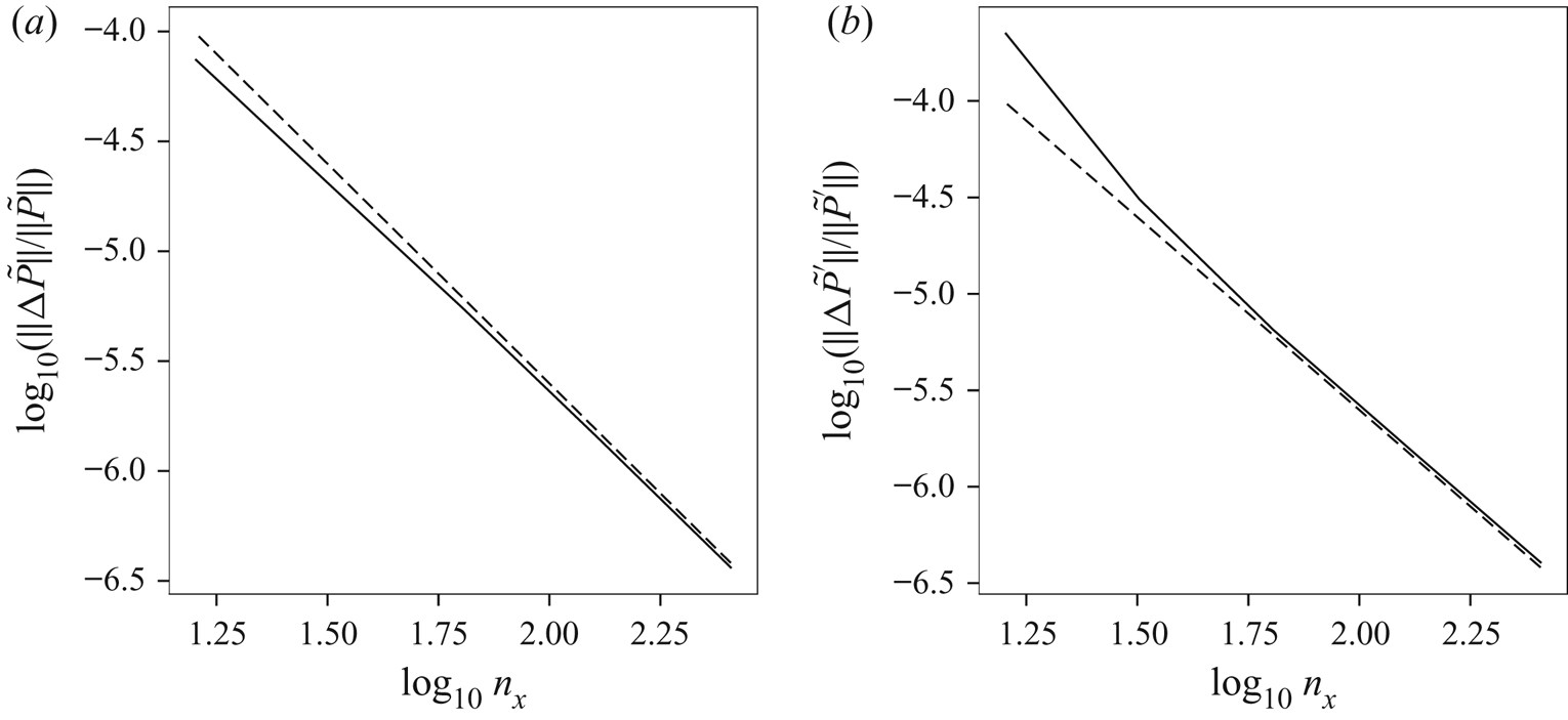
Appendix B. Time integration
This appendix provides details of the semi-implicit time stepping method used for all model equations. The method used is closely similar to that described in appendix C in DJ19, with the main differences coming from the forms of the nonlinear terms, owing to the different prognostic variable set  $({q_l},\delta ,\gamma _l)$ used here.
In general, the semi-implicit method is used to provide enhanced numerical stability at larger time steps when modelling systems containing high frequency waves, such as the free-surface gravity waves in the present context (Ritchie Reference Ritchie1988). In the linearised SW and 3-D equations, these waves have a maximum frequency  ${\sim }ck_{\textit{max}}$ at the largest horizontal wavenumber magnitude
 $k_{\textit{max}}$. An explicit method would need to resolve this frequency for numerical stability, but a semi-implicit method is unconditionally stable for any time step, at least for the linearised equations (accuracy for high frequency waves is sacrificed for stability on the assumption that these waves have negligible impact on the flow evolution).
For the linearised equations, the semi-implicit method is in fact fully implicit. For the nonlinear equations, this is no longer the case and the nonlinear ‘source’ terms must be evaluated from a previous estimate of the fields at the present and future time levels,  $n$ and
 $n+1$ (for a two-step method). Here, we follow the standard trapezoidal integration approach used previously in DJ19 (see appendix C), wherein the source terms are evaluated as a simple average of the two time levels. The future time level
 $n+1$ is repeatedly improved upon by iteration.
B.1. The 3-D model
The details of the method for the 3-D model equations are outlined next. We start by re-writing (2.36)–(2.38) as
 \begin{gather} \frac{{{\partial}} {{q_l}}}{{{\partial}} {t}} = {N_q}-\mathbb{D}{q_l}, \end{gather}
 \begin{gather} \frac{{{\partial}} {\delta}}{{{\partial}} {t}}-\gamma_l = {N_\delta}-\mathbb{D}\delta, \end{gather}
 \begin{gather} \frac{{{\partial}} {\gamma_l}}{{{\partial}} {t}}-\mathbb{G}\delta = {N_\gamma}-\mathbb{D}\gamma_l, \end{gather}
where  ${N_q}$,
 ${N_\delta }$ and
 ${N_\gamma }$ are the nonlinear source terms (the right-hand sides of (2.36)–(2.38)), and
 \begin{equation} \mathbb{D}=\nu(-\boldsymbol{\nabla}^{2})^{p} \end{equation}
is a hyper-diffusion operator used to absorb the nonlinear spectral cascade to small scales and prevent the build up of high wavenumber noise.
The term  $\mathbb {G}\delta$ in (B 3) couples the equations vertically, since the operator
 $\mathbb {G}$ defined in (2.40) involves a vertical integral. After a horizontal Fourier transform (
 $\boldsymbol{\nabla} ^{2}\to -k^{2}$) and discretising
 ${{\theta }}$ into
 $n_{{{\theta }}}$ equal layers, we use trapezoidal integration over
 ${{\theta }}$ to obtain
 \begin{equation} \mathbb{G}\delta_i={-}f^{2}\delta_i-c^{2}k^{2}\sum_{m=0}^{n_z}\mu_m\delta_m \end{equation}
on the surface  ${{\theta }}={{\theta }}_i=i{\rm \Delta} {{\theta }}$, where
 $\mu _0=\mu _{n_z}=1/(2n_z)$ and
 $\mu _m=1/n_z$ for
 $0<m<n_z$.
We next time discretise using the semi-implicit method. Time derivatives are evaluated by simple differences, i.e. for any field  $\xi$
 \begin{equation} \frac{{{\partial}} {\xi}}{{{\partial}} {t}} \approx \frac{\xi^{n+1}-\xi^{n}}{{\rm \Delta} t}, \end{equation}
where  $n$ and
 $n+1$ denote the time levels, while all remaining terms are time-averaged, i.e.
 \begin{equation} \bar{\xi}=\frac{1}{2}\left(\xi^{n}+\xi^{n+1}\right). \end{equation}
Then, using
 \[ \frac{\xi^{n+1}-\xi^{n}}{{\rm \Delta} t}=\omega_0\left(\bar{\xi}-\xi^{n}\right), \]
where  $\omega _0\equiv 2/{\rm \Delta} t$, and re-arranging (B 1)–(B 3) for the time averages
 $\bar {q}_{l,i}$,
 $\bar {\delta }_i$ and
 $\bar {\gamma }_{l,i}$, we obtain
 \begin{gather} \mathbb{R}\bar{q}_{l,i} = \tilde{N}_{q,i} \equiv \bar{N}_{q,i}+\omega_0{q_{l,i}}^{n}, \end{gather}
 \begin{gather} \mathbb{R}\bar{\delta}_i-\bar{\gamma}_{l,i} = \tilde{N}_{\delta,i} \equiv \bar{N}_{\delta,i}+\omega_0\delta_i^{n}, \end{gather}
 \begin{gather} \mathbb{R}\bar{\gamma}_{l,i}-\mathbb{G}\bar{\delta}_i = \tilde{N}_{\gamma,i} \equiv \bar{N}_{\gamma,i}+\omega_0\gamma_{l,i}^{n}, \end{gather}
where
 \begin{equation} \mathbb{R}=\omega_0+\mathbb{D} = \omega_0+\nu k^{2p} \end{equation}
in spectral space.
These equations are solved by iteration in order to improve the approximations to the nonlinear terms at time level  $n+1$. Initially, only quantities at time level
 $n$ are known, so we start with
 $\bar {N}_{q,i}=N_{q,i}^{n}$,
 $\bar {N}_{\delta ,i}=N_{\delta ,i}^{n}$ and
 $\bar {N}_{\gamma ,i}=N_{\gamma ,i}^{n}$ in (B 8)–(B 10). Equation (B 8) for
 $\bar {q}_{l,i}$ is decoupled from the other two and thus we have
 \[ \bar{q}_{l,i} = \mathbb{R}^{{-}1}\tilde{N}_{q,i} \]
directly. The remaining two equations for  $\bar {\delta }_i$ and
 $\bar {\gamma }_{l,i}$ are coupled, but they are easily combined to give
 \begin{gather} (\mathbb{R}^{2}-\mathbb{G})\bar{\delta}_i = \tilde{T}_{\delta,i} \equiv \mathbb{R}\tilde{N}_{\delta,i}+\tilde{N}_{\gamma,i}, \end{gather}
 \begin{gather} (\mathbb{R}^{2}-\mathbb{G})\bar{\gamma}_{l,i} = \tilde{T}_{\gamma,i} \equiv \mathbb{R}\tilde{N}_{\gamma,i}+\mathbb{G}\tilde{N}_{\delta,i} . \end{gather}
While the operator  $\mathbb {G}$ couples the equations vertically, their solutions are nevertheless straightforward:
 \begin{gather} \bar{\delta}_i = (\mathbb{R}^{2}+f^{2})^{{-}1}\left(\tilde{T}_{\delta,i}-\mathbb{F}\sum_{m=0}^{n_z}\mu_m\tilde{T}_{\delta,m}\right), \end{gather}
 \begin{gather} \bar{\gamma}_{l,i} = (\mathbb{R}^{2}+f^{2})^{{-}1}\left(\tilde{T}_{\gamma,i}-\mathbb{F}\sum_{m=0}^{n_z}\mu_m\tilde{T}_{\gamma,m}\right), \end{gather}
where
 \begin{equation} \mathbb{F}=\frac{c^{2}k^{2}}{\mathbb{R}^{2}+f^{2}+c^{2}k^{2}} \end{equation}
in spectral space. These solutions follow because the sums over  $m$ in (B 14) and (B 15) are independent of
 $i$ and the weights
 $\mu _m$ sum to unity. Alternatively, posing a solution of the form (B 14) and inserting it into (B 12) gives the form of
 $\mathbb {F}$.
From  $\bar {q}_{l,i}$,
 $\bar {\delta }_i$ and
 $\bar {\gamma }_{l,i}$, estimates for the fields at time level
 $n+1$ are obtained from
 \[ q_{l,i}^{n+1}=2\bar{q}_{l,i}-q_{l,i}^{n}, \quad \delta_i^{n+1}=2\bar{\delta}_i-\delta_i^{n}, \quad \gamma_{l,i}^{n+1}=2\bar{\gamma}_{l,i}-\gamma_{l,i}^{n}. \]
From these, we can obtain the corresponding velocity field and layer thicknesses by the inversion procedure described in § 2.3. Then all quantities are known that are needed to estimate the nonlinear terms at time level  $n+1$, giving an improved approximation to the time-averaged quantities
 $\bar {N}_{q,i}$,
 $\bar {N}_{\delta ,i}$ and
 $\bar {N}_{\gamma ,i}$ in (B 8)–(B 10). The above procedure is then repeated, in practice two more times, before the solution is accepted.
B.2. The 2-D models
The SW and GN model equations are solved similarly. In the SW model, the operator  $\mathbb {G}$ reduces to
 $-f^{2}-c^{2}k^{2}$ in spectral space (no vertical sum). Then (B 12) and (B 13) provide
 $\bar {\delta }$ and
 $\bar {\gamma }_l$ directly after division by
 $\mathbb {R}^{2}-\mathbb {G}$.
In the GN model, we make use of the diagnostic relation for  $\bar {P}_n$ in (3.14) to pull out the expected linear dispersion relation in the semi-implicit system. We begin by re-writing (3.16) and (3.17) as
 \begin{gather} \frac{{{\partial}} {\delta}}{{{\partial}} {t}}-\mathbb{P}^{{-}1}\gamma_l = {N_\delta} \equiv 2\delta^{2}-\boldsymbol{\nabla}\boldsymbol{\cdot}\left(\delta{{\boldsymbol{u}}}\right) +(H\mathbb{P})^{{-}1}\xi-\left(\frac{3}{h^{3}}-\frac{3}{H^{3}}\right)\bar{P}_n , \end{gather}
 \begin{gather} \frac{{{\partial}} {\gamma_l}}{{{\partial}} {t}}-\mathbb{G}\delta = {N_\gamma} \equiv \mathbb{G}\boldsymbol{\nabla}\boldsymbol{\cdot}({{\tilde{h}}}{{\boldsymbol{u}}}) -f\left[\boldsymbol{\nabla}\boldsymbol{\cdot}\left({q_l}{{\boldsymbol{u}}}\right)-J_{xy}(\bar{P}_n,h^{{-}1})\right], \end{gather}
where
 \begin{equation} \mathbb{P}=1+\tfrac 13 k^{2} H^{2} \end{equation}
in spectral space, and
 \begin{equation} \xi=h\tilde{\gamma}-H\gamma_l+\frac{\boldsymbol{\nabla}{h}\boldsymbol{\cdot}\boldsymbol{\nabla}{\bar{P}_n}}{h} +\left(\frac{3}{h^{2}}-\frac{3}{H^{2}}\right)\bar{P}_n \end{equation}
is the non-constant-coefficient part of the diagnostic relation for  $\bar {P}_n$, i.e.
 \begin{equation} \left(\boldsymbol{\nabla}^{2}-\frac{3}{H^{2}}\right)\bar{P}_n=H\gamma_l+\xi . \end{equation}
Equation (B 21) is solved iteratively, updating  $\xi$ after each iteration, until the r.m.s. difference between successive estimates of
 $\bar {P}_n$ falls below
 $10^{-11}$. Thus,
 $\xi$ is a product of this iteration, and is available for use in (B 17) for semi-implicit time stepping. The system of equations for
 $\bar {\delta }$ and
 $\bar {\gamma }_l$ takes the form
 \begin{gather} (\mathbb{P}\mathbb{R}^{2}-\mathbb{G})\bar{\delta} = \mathbb{P}\mathbb{R}\tilde{N}_{\delta}+\tilde{N}_{\gamma}, \end{gather}
 \begin{gather} (\mathbb{P}\mathbb{R}^{2}-\mathbb{G})\bar{\gamma}_l = \mathbb{P}(\mathbb{R}\tilde{N}_{\gamma}+\mathbb{G}\tilde{N}_{\delta}) . \end{gather}
Here, as in the 3-D equations,
 \begin{equation} \tilde{N}_{\delta} \equiv \bar{N}_{\delta}+\omega_0\delta^{n} \quad\text{and}\quad \tilde{N}_{\gamma} \equiv \bar{N}_{\gamma}+\omega_0\gamma_l^{n}, \end{equation}
where  $\bar {N}_{\delta }$ and
 $\bar {N}_{\gamma }$ are averages of the nonlinear source terms
 ${N_\delta }$ and
 ${N_\gamma }$ in (B 17) and (B 18).
Importantly, this approach differs from that taken in DJ19, who further simplified the semi-implicit system as advocated by Mohebalhojeh & Dritschel (Reference Mohebalhojeh and Dritschel2004) (see appendix B therein). The present approach, however, more accurately represents the effects of hyperdiffusion and significantly better controls the high wavenumber portion of field spectra in the GN equations (there is no significant improvement for the SW equations).
Appendix C. Numerical parameter settings
In all models, we use identical parameter settings to those used in DJ19. We use  $n_x=n_y=n_h$ horizontal grid points with
 $n_h=256$ or
 $512$, and in the 3-D simulations we use
 $n_{{{\theta }}}=32$ or
 $64$ grid intervals (or
 $n_{{{\theta }}}+1$ grid points, two of which lie on the boundaries). The time step is set to
 ${\rm \Delta} t=0.32{\rm \Delta} x/c$, where
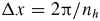 ${\rm \Delta} x=2{\rm \pi} /n_h$ is the grid spacing and
 $c=\sqrt {gH}$. This allows one to marginally resolve the highest frequency gravity wave in the 3-D and SW simulations (such waves have lower frequencies in the GN model, see DJ19).
To absorb the natural nonlinear cascade to small (horizontal) scales, third-order hyperdiffusion of the form  $\nu \boldsymbol{\nabla}^{6}$ is added to each prognostic equation with
 \[ \nu=\frac{10f}{(n_h/2)^{6}} , \]
corresponding to a damping rate of  $10$ per inertial period
 $2{\rm \pi} /f$ at the smallest resolved scale (see DJ19). Notably, no vertical diffusion is added.