1. Introduction
Financial markets unite, transmit, and present information from the economy to individuals and companies. Fluctuations in financial markets, in turn, can trigger subsequent changes in the economy, impacting various economic segments. One potential source of fluctuation in financial markets is the escalating risk posed by climate change (Felbermayr et al. Reference Felbermayr, Gröschl, Sanders, Schippers and Steinwachs2022).
The literature has documented the widespread effects of climate change. Subak et al. (Reference Subak, Palutikof, Agnew, Watson, Bentham and Cannell2000), Felbermayr et al. (Reference Felbermayr, Gröschl, Sanders, Schippers and Steinwachs2022), and Chen et al. (Reference Chen, Zhang and Chen2024) show that weather anomalies and extreme temperatures negatively impact economic activity by reducing industrial and agricultural production, hindering entrepreneurship, and affecting energy consumption. Aslan et al. (Reference Aslan, Altinoz and Polat2024) further argue that climate change reduces investment, innovation, and labor productivity in Europe.
In financial markets, Cao and Wei (Reference Cao and Wei2005) and Taşkin et al. (Reference Taşkin, Cagli and Evrim Mandaci2021) document that climate change influences stock and futures markets. Attilio et al. (Reference Attílio, Faria and McAdam2025) examine a dynamic IS-LM open economy model extended with the Green Tobin q (Faria et al. Reference Faria, Tindall and Terjensen2022). They analyze the effect of monetary and green patenting shocks across the G7 countries. Both shocks influence green patents through real and financial markets. Results to green patent shocks suggest an over time trade-off between promoting pollution reduction and energy efficiency and profitability. Despite these findings, a gap remains in understanding how climate change propagates across economic sectors, ultimately affecting production. This study aims to address that gap.
We explore this possibility in this paper, investigating the impact of climate change on financial markets within a system of multiple economies. We define climate change as increases in temperature anomalies and examine the responses of four key financial markets: stock markets, exchange markets, short-term credit markets, and long-term credit markets. Throughout our analysis, we aim to capture spillover effects, transmission channels, and heterogeneities.
Our hypothesis posits that temperature anomaly shocks impact economies through financial markets, which then transmit the shock to production.
Thus, our research goal is to detect the impact of temperature anomalies on financial markets. Additionally, as we explain in the paper, our econometric approach allows us to explore: i) spillover effects, ii) transmission channels, and iii) heterogeneities. Spillover effects may be detected through the responses of economies to temperature anomalies; we analyze how temperature shocks spread over economies. Transmission channels provide an explanation and rationale for how economic sectors affect each other. For example, we analyze how financial markets can transmit a noneconomic shock (temperature shock) to production. Finally, since Global VAR (GVAR) is a set of individual models, we can verify how each model responds to temperature shocks, highlighting heterogeneities. Naturally, points i, ii, and iii are empirical possibilities, which help us to accomplish our research goal and contribute to the literature.
We employ the GVAR model in the empirical section. There are three reasons for using this model. Firstly, it treats climate change as an externality, wherein a shock to climate change reverberates across all countries, inducing fluctuations in their variables. Secondly, GVAR constructs individual models for each economy and interlinks them through economic integration variables. Given that climate change exerts global impacts, GVAR accommodates this characteristic. Thirdly, owing to these considerations, GVAR captures spillover effects, transmission channels, and heterogeneities. We use the GVAR with a sample comprising 20 economies spanning from January 1999 to January 2023.
The merit of GVAR lies in its ability to integrate these three characteristics within the same framework. Panel data unites multiple economies and yields statistically significant relationships. However, it provides a single coefficient for the entire sample, hiding heterogeneities. Another limitation is its failure to capture spillover effects. Panel Vector Autoregressive (PVAR) addresses spillover effects but, akin to panel data, overlooks heterogeneities in the shocks analyzed.
VAR (Vector Autoregressive) models, along with others like Structural VAR (SVAR) and Vector Error Correction (VEC), capture spillover effects and depict individual countries’ responses to shocks. Nonetheless, these models focus solely on a single economy. Consequently, we opted for GVAR due to its capacity to incorporate multiple economies, capture spillover effects, and generate heterogeneities. Additionally, it enables the analysis of potential transmission channels, providing insights into the fluctuations induced by climate change shocks.
The results reveal that temperature anomalies exert an influence on financial markets, inflation, and production. We observed that domestic currencies depreciate, stock markets experience devaluation, and long-term interest rates decline. The estimates suggest minor fluctuations in short-term interest rates. These shifts propagate the shock to production, resulting in declines in industrial production. Subsequently, domestic prices decrease. Consequently, the main finding is that climate change negatively affects industrial production through four potential financial channels.
These findings indicate the presence of spillover effects of climate change on economies, with financial markets serving as potential channels for the shock. Furthermore, we detected heterogeneities, for example the heightened sensitivity of industrial production in the Eurozone, U.K., and U.S. compared to other economies. However, one common characteristic in most economies is the stock market transmitting the temperature anomaly shock to production. This is the main transmission channel and, therefore, the most sensitive financial market to climate change.
The literature indicates that climate change impacts financial markets (Cao and Wei, Reference Cao and Wei2005; Makkonen et al. Reference Makkonen, Vallström, Uddin, Rahman and Haddad2021; Lee et al. Reference Lee, Mark, Nauerz, Rawls and Wei2022). Previous studies have employed panel data, PVAR, and time series methods, but these approaches often overlook spillover effects and heterogeneities. Additionally, they typically do not treat climate change as an externality. Another limitation is the absence of a comprehensive framework to depict interactions among financial markets.
To address these gaps, we incorporate four financial markets (stock, exchange, short-term credit, and long-term credit markets) into our analysis. We recognize the interconnectedness of domestic and international financial markets, considering feedback and second-round effects. This approach enriches our analysis by providing more detailed insights.
In addition to financial markets reacting to climate change, the literature suggests that production and inflation also respond to shifts in global temperatures (Farajzadeh et al. Reference Farajzadeh, Ghorbanian and Tarazkar2022; Berg et al. Reference Berg, Curtis and Mark2023; Khalfaoui et al. Reference Khalfaoui, Goodell, Mefteh-Wali, Chishti and Gozgor2024). We expand on these studies by incorporating production and inflation into our model, linking them with the four financial markets across 20 economies. This framework enables us to elucidate the propagation of climate change shocks, with financial markets serving as potential transmission channels.
Colacito et al. (Reference Colacito, Hoffmann and Phan2019), Ali et al. (2022), Hunjra et al. (Reference Hunjra, Azam and Al-Faryan2022), Faria et al. (Reference Faria, McAdam and Viscolani2023), and Apergis and Rehman (Reference Apergis and Rehman2024) demonstrated the impact of climate change on economic growth and financial policy uncertainty using panel data. However, as we have contended, these inquiries fail to integrate crucial elements of the climate change phenomenon. By disregarding the spillover effects of climate change, the estimates may exhibit bias. Furthermore, while these studies highlight relationships between a proxy for climate change and an economic variable, they do not provide a comprehensive overview of the cascading effects of climate change on economies.
Regarding the literature, our paper’s novelty lies in constructing a framework for open economies where temperature anomaly shocks propagate through financial markets, production, and inflation. This is achievable because we modeled climate change as an externality capable of instigating changes across multiple economies. Consequently, our model offers insights into transmission channels, spillover effects, and heterogeneities associated with temperature anomaly shocks.
Our results contribute to the discussion on climate change and its economic impact by detecting channels through which it influences goods markets. We argue that climate change affects financial markets, which, in turn, transmit these effects to goods markets. In this context, our study establishes a link between financial and goods markets, offering a rationale for the broader dissemination of climate change effects across countries.
We structured this paper as follows: Section 2 discusses the literature review, Sections 3 and 4 construct the theoretical model, Section 5 presents the results, and Section 6 concludes the investigation.
2. Literature review
The literature on climate change demonstrates its impact on financial markets. Cao and Wei (Reference Cao and Wei2005) analyzed the stock markets of nine economies, revealing statistically significant relationships between these markets and temperature anomalies through panel regressions. Lee et al. (Reference Lee, Mark, Nauerz, Rawls and Wei2022) demonstrated that temperature anomalies affect the exchange rates of 76 countries using local projections. Mukherjee and Ouattara (Reference Mukherjee and Ouattara2021) argued that temperature shocks stimulate prices, causing changes in inflation and subsequently in monetary policy, as central banks are committed to stable prices. They used a PVAR from 1961 to 2014 in a sample of 107 countries to support their claim. Makkonen et al. (Reference Makkonen, Vallström, Uddin, Rahman and Haddad2021) employed quantile regressions to illustrate that temperature anomalies cause changes in stock markets and exchange rates, reinforcing the findings of Cao and Wei (Reference Cao and Wei2005) and Lee et al. (Reference Lee, Mark, Nauerz, Rawls and Wei2022).
There are three limitations in these studies. The first is the nature of climate change. Climate change presents two market failures: public goods and externalities. In this context, public goods represent the benefits a country can derive from the adoption of policies from other countries. If a country reduces its carbon emissions, contributing to reducing the global temperature, other countries may benefit, even though they did not contribute to this result. Externalities show that the carbon emissions of a country affect its neighbors. In other words, climate change transcends national boundaries. The second limitation derives from the first point: climate change has spillover effects. Thus, most studies do not incorporate these considerations into their econometric models.
The regressions used by Cao and Wei (Reference Cao and Wei2005) ignored the spillover effects of climate change on the variables. The PVAR applied in Mukherjee and Ouattara (Reference Mukherjee and Ouattara2021) captures part of the spillover effects, but the method does not fully portray the chain reaction resulting from the dissemination of temperature shocks. Consequently, we encounter the third limitation: the lack of a rationale behind the results. A question such as “how does a temperature anomaly shock affect economies?” remains unanswered.
We contribute by employing the GVAR. GVAR constructs individual models for each economy and connects them using integration variables. Thus, GVAR models climate change as a variable capable of causing spillover effects. GVAR allows us to include several variables in the individual models. We incorporate financial markets to bridge the temperature anomaly shock on economies. The rationale is that temperature shock provokes changes in financial markets, and their reactions transmit the shock to production. These are the potential transmission channels. We also include long-term credit markets—in addition to the stock market, the exchange market, and the short-term credit market—a component of financial markets that the literature has given little attention to until now.
Besides the impact of temperature shocks on financial markets, Farajzadeh et al. (Reference Farajzadeh, Ghorbanian and Tarazkar2022), Felbermayr et al. (Reference Felbermayr, Gröschl, Sanders, Schippers and Steinwachs2022), Berg et al. (Reference Berg, Curtis and Mark2023), and Khalfaoui et al. (Reference Khalfaoui, Goodell, Mefteh-Wali, Chishti and Gozgor2024) have shown that climate change affects inflation and production. This is an expected progression in the literature, given the understanding that climate change influences financial markets.
However, there is an absence of an econometric model connecting temperature anomalies to financial markets, production, and inflation. We fill this gap by adopting the GVAR in a system of 20 economies. We use bilateral trade to represent a framework of open economies. These economies are vulnerable to external shocks, such as temperature anomaly shocks. Therefore, we provide transmission channels, capture spillover effects, and treat climate change as both a public good and an externality. Finally, since we employ a system of individual models, the estimates exhibit heterogeneities.
In summary, this paper offers both theoretical and empirical contributions. Theoretically, it proposes that climate change affects production through its influence on financial markets, positioning financial markets as transmission channels for climate change.
Empirically, the model links multiple economies through financial and goods markets, illustrating the impact of climate change on production while considering financial markets as potential transmission mechanisms. Together, these models address a gap in the literature regarding the connections between climate change, financial markets, and production fluctuations.
Both models account for asymmetry, regime changes, and time-varying effects. In particular, the empirical model captures these dynamics by providing the individual responses of each economy to a global shock.
3. The baseline model
We study an open macroeconomic model based on Blanchard (Reference Blanchard1981) and Attílio et al. (Reference Attílio, Faria and Rodrigues2023). We develop a model of the determination of output, the stock market and the term structure of interest rates. The model we present focuses on macroeconomic variables, particularly financial markets. It does not explore individual behaviors through utility functions and budget constraints; hence, it does not have a microeconomic foundation. We adopt a macroeconomic perspective to analyze the impact of temperature anomalies on a set of economies.
There are four determinants of spending: 1) values of shares in the stock market q, which is part of wealth; 2) current income y that is affected by temperature anomalies A which are, a priori, ambiguous, since in some regions it can be positive and in others negative; 3) fiscal policy, both through taxes and public spending, g; 4) Net trade balance which is impacted by variations in the exchange rate,
 $\varepsilon$
. Total spending is:
 \begin{equation}d=aq+\beta y\left(A\right)+g+NX(\varepsilon );\,a\gt 0;\,\beta \in [0,1)\end{equation}
All variables are real. Output adjusts to spending over time:
 \begin{equation}\dot{y}=\sigma \left(aq+\beta y\left(A\right)+g+NX(\varepsilon )-y\left(A\right)\right)=\sigma \left(aq+g+NX(\varepsilon )-by\left(A\right)\right);\, b=1-\beta \gt 0\end{equation}
where a dot represents a time derivative. In the steady-state (3.2) yields the equilibrium in the goods market.
The equilibrium in the money market is given by the conventional LM relation, which can be written as:
 \begin{equation}i=cy\left(A\right)-h\left(m-p\right)\!;\quad c\gt 0;\quad h\gt 0\end{equation}
where i denotes the short-term nominal rate of interest, m and p are, respectively, logs of nominal money and the price level. The short-term real interest rate r is defined as:
 \begin{equation}r=i-\dot{p}*\end{equation}
where
 $\dot{p}*$
is the expected inflation rate.
The long-term bonds are consols with yield I and price 1/I. The expected short-term nominal rate of return from holding consols is the sum of the yield and the expected nominal capital gain, so we have:
 \begin{equation}\mathrm{I}\left[1+\frac{{\rm d}}{{\rm d}t}\left(\frac{1}{I}\right)\right]=i\rightarrow \frac{1}{I}\frac{{\rm d}I}{{\rm d}t}=I-i\end{equation}
The long-term real rate R is defined similarly:
 \begin{equation}\frac{1}{R}\frac{dR}{dt}=R-r\end{equation}
The expected rate of return on holding shares is the growth rate of q plus the rate of real profit
 $\pi$
and q. Real profit is an increasing function of income:
 \begin{equation}\pi =\alpha _{0}+\alpha _{1}y(A)\end{equation}
Arbitrage between short-term bonds and shares yields:
 \begin{equation}\frac{1}{q}\frac{dq}{dt}+\frac{\alpha _{0}+\alpha _{1}y\left(A\right)}{q}=r\end{equation}
4. The Steady state equilibrium with fixed prices
Assuming prices are fixed there is no actual and expected inflation and by Eq. (3.4) nominal and real rates of interest are equal:
 \begin{equation}r=i \end{equation}
Therefore, the LM determines the equilibrium r:
 \begin{equation}r=cy\left(A\right)-h\left(m-p\right)\end{equation}
It is important to stress that by Eq. (4.2) a variation in temperature anomalies A, changes output, which affects r, that is:
 \begin{equation}\frac{{\rm d}r}{{\rm d}A}=c\, \frac{{\rm d}y\left(A\right)}{{\rm d}A}\end{equation}
In the steady-state all endogenous variables are constant, therefore given r, Eq. (3.6) determines the equilibrium value of R:
 \begin{equation}r=R\end{equation}
According to (3.3), (4.1) and (4.3) temperature anomalies also affect nominal interest rates i and long-term real rate R:
 \begin{equation}\frac{{\rm d}i}{{\rm d}A}=c\, \frac{{\rm d}y\left(A\right)}{{\rm d}A};\quad \frac{{\rm d}R}{{\rm d}A}=c\, \frac{{\rm d}y\left(A\right)}{{\rm d}A}\end{equation}
Given equilibrium r in the steady-state in Eq. (3.8) determines the equilibrium value of q:
 \begin{equation}q=\frac{\alpha _{0}+\alpha _{1}y\left(A\right)}{r}\end{equation}
Note that according to Eq. (4.6) temperatures anomalies impact the real value of the stock market direct and indirectly:
 \begin{equation}\frac{{\rm d}q}{{\rm d}A}=\left[\frac{\alpha _{1}}{r}-c\frac{\alpha _{0}+\alpha _{1}y\left(A\right)}{r}\right]\frac{{\rm d}y\left(A\right)}{{\rm d}A}\end{equation}
Given equilibrium q, in the steady state Eq. (3.2) determines the equilibrium value of the exchange rate,
 $\varepsilon$
[real and nominal since prices are constant]:
 \begin{equation}NX\left(\varepsilon \right)=by\left(A\right)-g-aq\end{equation}
Therefore, the exchange rate is also affected by temperature anomalies direct and indirectly:
 \begin{equation}\frac{{\rm d}\varepsilon }{{\rm d}A}=NX'\left(\varepsilon \right)^{-1}\, \left\{b-a\left[\frac{\alpha _{1}}{r}-c\frac{\alpha _{0}+\alpha _{1}y\left(A\right)}{r}\right]\right\}\frac{{\rm d}y\left(A\right)}{{\rm d}A}\end{equation}
Finally given Eq. (4.1) and the steady state of Eq. (3.5) determines the equilibrium value of the yield of long-term bonds:
 \begin{equation}I=i\end{equation}
As a consequence I is also impacted by A:
 \begin{equation}\frac{{\rm d}I}{{\rm d}A}=c\, \frac{{\rm d}y\left(A\right)}{{\rm d}A}\end{equation}
Our model shows that temperature anomalies A impact all endogenous variables of our model: r, i, R, I, q, and
 $\varepsilon$
. In particular we are concerned about the effect of temperature anomalies on four financial markets (exchange rate, stock market, and short- and long-term credit markets).
Empirical studies support these connections. Cao and Wei (Reference Cao and Wei2005), Peillex et al. (Reference Peillex, El Ouadghiri, Gomes and Jaballah2021), and Makkonen et al. (Reference Makkonen, Vallström, Uddin, Rahman and Haddad2021) argue that temperature anomalies affect stock markets by influencing the mood of individuals, leading to a higher inclination towards aggression, apathy, and tiredness, which in turn changes their risk-taking behavior. Another channel is the risk faced by farmers: unfavorable weather can reduce agricultural production, prompting farmers to hedge this risk by selling their produce in future markets. However, these markets incorporate several macroeconomic variables that may affect the harvest, including temperature anomalies.
Regarding credit markets, Tzouvanas et al. (Reference Tzouvanas, Kizys, Chatziantoniou and Sagitova2019), Felbermayr et al. (Reference Felbermayr, Gröschl, Sanders, Schippers and Steinwachs2022), and Aguilar-Gomez et al. (Reference Aguilar-Gomez, Gutierrez, Heres, Jaume and Tobal2024) showed that temperature anomalies increase the risk of natural catastrophes such as floods, excessive precipitation, and droughts. These events negatively impact not only agricultural production but also other sectors. Depending on the scope of the climatic change, entire economic sectors may be adversely affected. This dynamic can create systemic risk, spreading these effects throughout the economy. Lower production, decreasing revenues, and higher costs push companies into financial stress, contributing to higher interest rates. Additionally, these studies documented lower labor productivity, higher absenteeism, and a decline in the willingness to spend among the population, which reinforces unfavorable business cycles through supply and demand variables, ultimately affecting credit markets and default rates.
Since currency markets capture the risk perception of individuals and companies regarding future events, changes in temperature anomalies trigger reactions in exchange rates (Lee et al. Reference Lee, Mark, Nauerz, Rawls and Wei2022; Bonato et al. Reference Bonato, Cepni, Gupta and Pierdzioch2023). The aforementioned studies describe capital movements due to global warming, which may contribute to higher volatility in exchange rates, as currencies are sensitive to capital flows. Thus, exchange rates can respond to temperature anomalies due to the perception of higher risk in macroeconomic fundamentals and the chain reaction promoted by changes in capital allocation.
5. Methodology and data
We employ the GVAR model in our analysis. This model consists of individual VARXs (VAR models with foreign variables) for each region i in time t. Equation (5.1) describes a VARX with one lag for the domestic (
 $x_{it}$
) and foreign variables (
 $x_{it}^{*}$
). The other terms are the constant,
 $a_{i0}$
; the trend,
 $a_{i1}t$
; and the vector of idiosyncratic shocks,
 $\varepsilon _{it}$
.
 \begin{equation}x_{it}=a_{i0}+a_{i1}t+\Phi _{i}x_{i,t-1}+\Lambda _{i0}x_{it}^{*}+\Lambda _{i1}x_{i,t-1}^{*}+\varepsilon _{it}.\end{equation}
We connect the economies using foreign variables. Equation (5.2) presents the construction of these variables. We use bilateral trade between regions i and j,
 $w_{ij}$
. Besides linking economies, foreign variables possess at least two essential characteristics for our research. Firstly, foreign variables simulate the international economy, serving as a proxy for the external scenario. Secondly, they represent constraints on the equilibrium of economies. This latter characteristic is referred to as weak-exogeneity.
 \begin{equation}x_{it}^{*}=\sum _{j=0}^{N}w_{ij}x_{jt}.\end{equation}
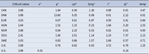
We tested whether foreign variables are weakly exogenous using the weak exogeneity test (see Table A5 in the Appendix). The results showed that most foreign variables are weakly exogenous. Additionally, we used time-varying bilateral trade to accommodate changes in variables and potential structural changes in trade (see Section 6.4) . For example, for the foreign variable of the year 1999, we used the average of bilateral trade in the years 1999, 2000, and 2001 to construct it. In other words, time-varying bilateral trade uses moving averages to incorporate changes in trade in the construction of foreign variables.
Most GVAR empirical studies use bilateral trade to connect economies and create foreign variables (Pesaran et al. Reference Pesaran, Schuermann and Weiner2004; Considine et al. Reference Considine, Galkin, Hatipoglu and Aldayel2023). An alternative is to use bilateral financial flows (Eickmeier and Ng, Reference Eickmeier and Ng2015). Since we already include four financial markets in the empirical model, our model implicitly incorporates financial links. Bilateral trade provides another possible connection between economies. However, using bilateral trade to construct foreign variables is not perfect because it does not consider other relevant characteristics of economies, such as Gross domestic product (GDP) and population size. Nonetheless, bilateral trade is reasonable as a proxy for connecting economies due to the relevance of trade in spreading local shocks to other economies.
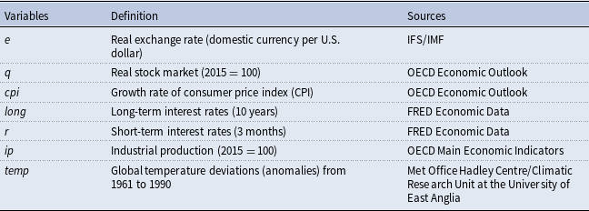
Table 1 presents the data. We use four variables to represent financial markets. The first variable is the real exchange rate sourced from the International Financial Statistics (IFS) of the International Monetary Fund (IMF). We adjusted this variable using the consumer price index (CPI) from the Organization for Economic Cooperation and Development (OECD) Economic Outlook. The exchange rate indicates the ratio of domestic currency per U.S. dollar.
Variables and sources

The second financial market proxy is the stock market value sourced from the OECD Economic Outlook. Similar to the exchange rate, we adjusted this time series using CPI. The third and fourth proxies represent short- and long-term credit markets, respectively. For short-term credit markets, we used the 3-month interbank rates and treasury securities, while for long-term credit markets, we employed 10-year government bonds. Both time series were collected from the Federal Reserve Bank of St. Louis (FRED) Economic Data.
Building upon previous studies that explore fluctuations in financial markets (Dees et al. Reference Dees, Mauro, Pesaran and Smith2007; Attílio et al. Reference Attílio, Faria and Rodrigues2023), we augmented the model by incorporating the growth rate of CPI (inflation) and industrial production. Industrial production data was sourced from the OECD Main Economic Indicators.
We collected the temperature anomaly data from the Met Office Hadley Centre/Climatic Research Unit at the University of East Anglia. This variable illustrates climate change by indicating global temperature deviations from the period 1961–1990.
The literature has shown that temperature anomalies may affect credit markets (Felbermayr et al. Reference Felbermayr, Gröschl, Sanders, Schippers and Steinwachs2022; Aguilar-Gomez et al. Reference Aguilar-Gomez, Gutierrez, Heres, Jaume and Tobal2024), stock markets (Cao and Wei, Reference Cao and Wei2005; Makkonen et al. Reference Makkonen, Vallström, Uddin, Rahman and Haddad2021), and exchange rates (Bonato et al. Reference Bonato, Cepni, Gupta and Pierdzioch2023). Thus, we included these variables in our analysis. Felbermayr et al. (Reference Felbermayr, Gröschl, Sanders, Schippers and Steinwachs2022) and Berg et al. (Reference Berg, Curtis and Mark2023) concluded that temperature anomalies impact production, so we incorporated this relationship by including industrial production. Finally, Ciccarelli et al. (Reference Ciccarelli, Kuik and Hernández2024) demonstrated that temperature shocks influence inflationary pressure, which we addressed by using the CPI.
Our period spans from 1999M1 to 2023M1, encompassing a sample of 20 economies: Austria (AUT), Belgium (BEL), Canada (CAN), Denmark (DNK), Finland (FIN), France (FRA), Germany (GER), Greece (GRE), Hungary (HUN), Ireland (IRL), Italy (ITA), Luxembourg (LUX), the Netherlands (NLD), Norway (NOR), Portugal (PRT), South Africa (SOU), Spain (SPA), Sweden (SWE), the United Kingdom (U.K.), and the United States (U.S.). Following the methodology of Dees et al. (Reference Dees, Mauro, Pesaran and Smith2007) and Attílio et al. (Reference Attílio, Faria and Rodrigues2023), we constructed the Eurozone (EUR) by aggregating economies (AUT, BEL, FIN, FRA, GER, GRE, IRL, ITA, LUX, NLD, PRT, and SPA) based on the average real GDP in PPP for the years 2019–2021, sourced from the World Development Indicators (WDI) of the World Bank. To construct the foreign variables and estimate the model, we used bilateral trade data from the Direction of Trade Statistics of the IMF.
We selected the period and sample based on data availability, with particular attention to information on financial markets, which influenced the number of countries, especially regarding long-term interest rates. Therefore, the databases provided by FRED and OECD were central in defining both our sample and period.
Equation (5.3) presents the domestic and foreign variables:
 \begin{equation*} x_{it}=\left(e_{it},q_{it},r_{it},long_{it},cpi_{it},ip_{it}\right) \end{equation*}
 \begin{equation}x_{it}^{*}=\left(q_{it}^{*},r_{it}^{*},long_{it}^{*},cpi_{it}^{*},ip_{it}^{*},temp_{it}^{*}\right).\end{equation}
In Eq. (5.3),
 $e_{it}$
is the real exchange rate;
 $q_{it}$
is the real stock market;
 $r_{it}$
is the short-term interest rate;
 $long_{it}$
is the long-term interest rate;
 $cpi_{it}$
is the inflation;
 $ip_{it}$
is industrial production; and the temp is temperature anomaly. According to Eq. (5.3), we connected the economies in all financial markets (foreign variables).
We adapted Eq. (5.3) for the U.S. Modifying the U.S. model is a recommendation in GVAR studies (Dees et al. Reference Dees, Mauro, Pesaran and Smith2007; Attílio et al. Reference Attílio, Faria and Rodrigues2023). According to Pesaran et al. (Reference Pesaran, Schuermann and Weiner2004) and Dees et al. (Reference Dees, Mauro, Pesaran and Smith2007), due to the role of the U.S. in international markets, the weak exogeneity assumption of the foreign variables could cause problems in the estimation. Weak exogeneity implies that countries may affect foreign variables while they respond to shocks. However, in the equilibrium of the model, these countries adjust to foreign variables. This assumption is too strong for an economy such as the U.S. Thus, we accommodate the U.S. model by reducing the number of foreign variables.
We included the exchange rate as a domestic variable for all economies, while treating it as a foreign variable in the U.S. model. We did this because the exchange rate is the ratio of domestic currency to the U.S. dollar. Other GVAR empirical studies also apply this configuration (Pesaran et al. Reference Pesaran, Schuermann and Weiner2004; Dees et al. Reference Dees, Mauro, Pesaran and Smith2007). The rationale behind this choice is that the exchange rate as a domestic variable already portrays the influence of the world economy; thus, there is no necessity to include this variable as a foreign variable. For the U.S., the influence of exchange rates is indirectly captured due to the inclusion of these variables in the other individual models.
Additionally, we introduced the global variable, temperature anomaly, as a domestic variable solely in the U.S. model. Another difference is that we incorporated two foreign variables in the U.S. model (exchange rate and industrial production), while six foreign variables were used for the rest of the regions (as described in Eq. 5.3).
As indicated by Eq. (5.2), in GVAR analysis, we use bilateral trade data to construct the international scenario and estimate the model. Typically, GVAR studies employ a three-year window for bilateral trade (Dees et al. Reference Dees, Mauro, Pesaran and Smith2007; Attílio et al. Reference Attílio, Faria and Rodrigues2023). In our approach, we adopt a three-year average of bilateral trade data. However, we employ two different strategies.
We aim to assess whether trade integration contributes to explaining the financial market fluctuations attributed to temperature anomalies. Our approach involves constructing two models: one utilizing bilateral trade from the years 2020 to 2022, and the other employing bilateral trade from the years 1999 to 2001. This allows us to examine whether structural changes in trade dynamics account for macroeconomic fluctuations.
The second approach involves using time-varying bilateral trade to calculate the foreign variable and, consequently, construct the international economy. This strategy incorporates structural changes in trade integration. The procedure entails using the moving average of bilateral trade to build foreign variables for each observation. For instance, the model constructs the foreign variable for 1999 using the average of 1999–2001, the foreign variable for 2000 using 2000–2002, and the foreign variable for 2001 using 2001–2003.
We use the Generalized Impulse Response Function (GIRF) to examine the effects of temperature anomaly shocks on domestic financial markets. GIRFs depict how the system responds to a shock, highlighting potential transmission channels and spillover effects. Unlike identifying shocks, GIRFs focus on illustrating these reactions. They serve as an alternative in scenarios with a large number of economies and domestic variables (Dees et al. Reference Dees, Mauro, Pesaran and Smith2007)
We additionally employ the Generalized Forecast Error Variance Decomposition (GFEVD) to gauge the impact of temperature anomalies on the decomposition of domestic variables. The GFEVD enables us to compare the significance of domestic factors and the external scenario in shaping the dynamics of domestic economies.
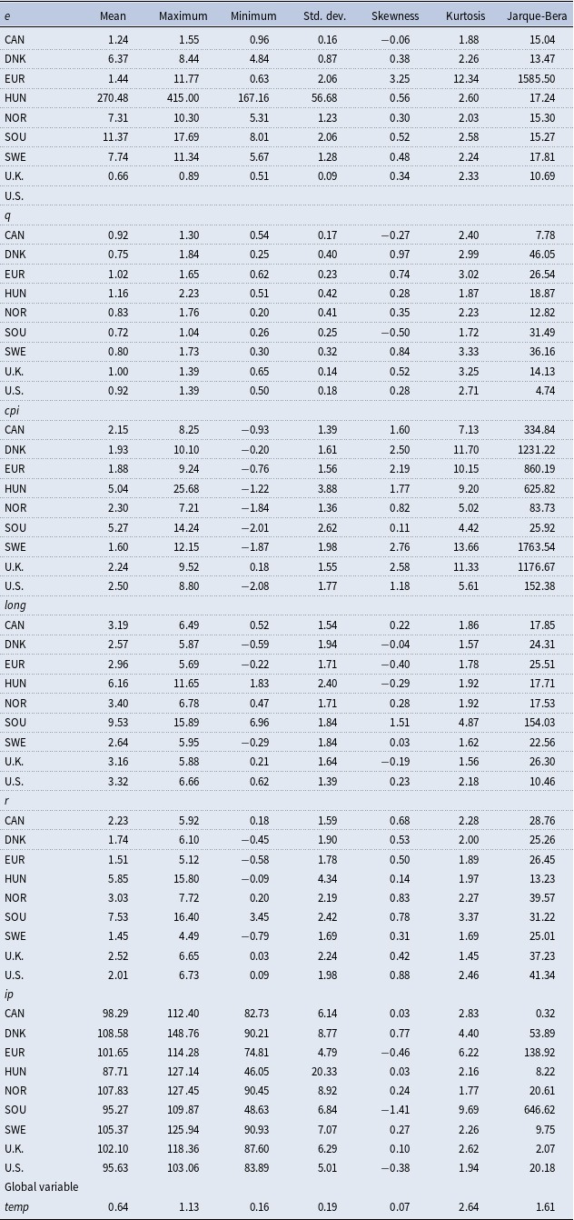
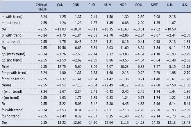
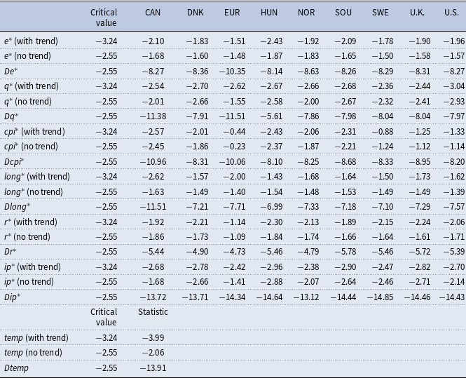
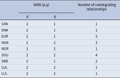
In the Appendix, Table A1 presents the descriptive statistics of the variables, while Tables A2 and A3 display the unit-root tests for domestic, foreign, and global variables. Tables A2 and A3 demonstrate the presence of unit roots in the time series. However, these time series become stationary when differenced once. Given the identification of cointegrating relationships in Table A4, we use the GVAR in the error correction form (see Pesaran et al. Reference Pesaran, Schuermann and Weiner2004). Additionally, Table A4 provides information on the lags for the VARX models, determined using the Akaike Information Criterion (AIC). Table A5 tests the hypothesis of weak exogeneity. The results confirm this hypothesis, indicating that foreign variables serve as long-term constraints to the equilibrium of economies.
6. Econometric results
6.1 Temperature anomaly shock
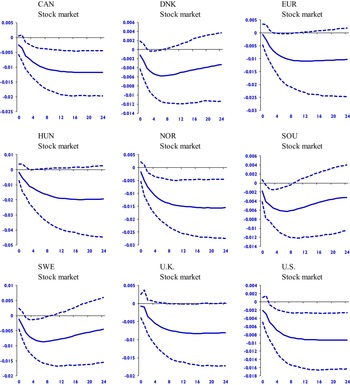
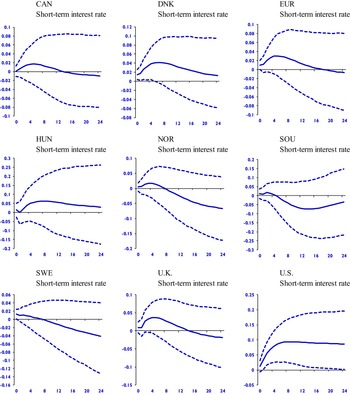
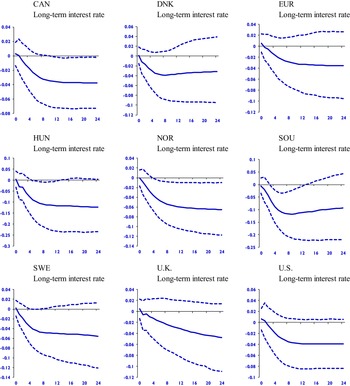
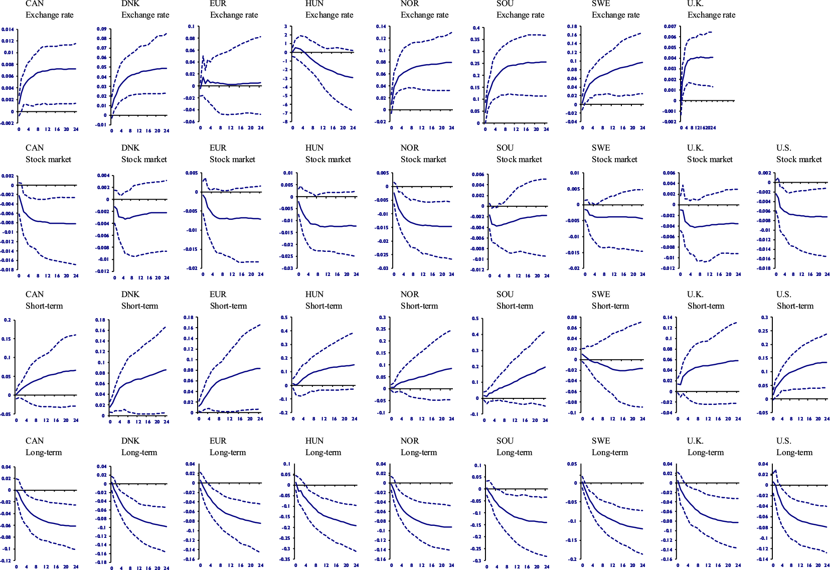
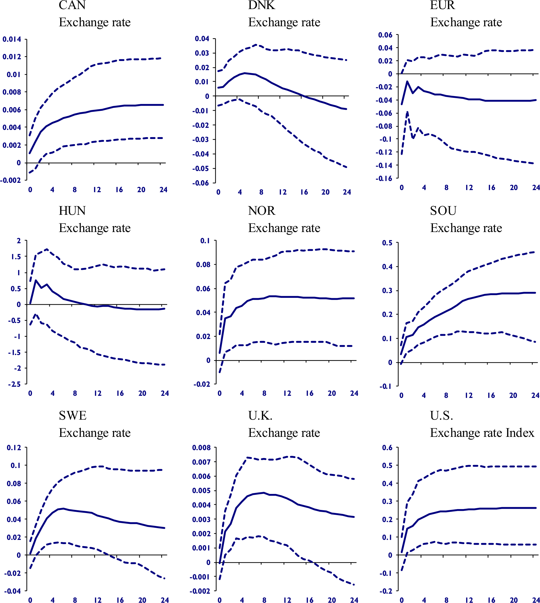
In this section, we analyze one standard deviation temperature anomaly shock and the responses of the four financial markets (exchange rates, stock markets, and short- and long-term credit markets), industrial production, and inflation. As mentioned in the previous section, we use bilateral trade data from the years 2020 to 2022 to estimate and solve the model. We test the robustness of the results using alternative bilateral trade years (Section 6.3) and time-varying bilateral trade (Section 6.4). Figures 1, 2, 3, and 4 present the GIRFs of the responses of financial markets. The dashed lines represent confidence intervals at 90%, calculated by bootstrap.
GIRF of temperature anomaly shock and responses of exchange rates.
Note: The U.S. does not have estimates because of the reasons we discussed in Section 5.

GIRF of temperature anomaly shock and responses of stock markets.

GIRF of temperature anomaly shock and responses of short-term interest rates.

GIRF of temperature anomaly shock and responses of long-term interest rates.

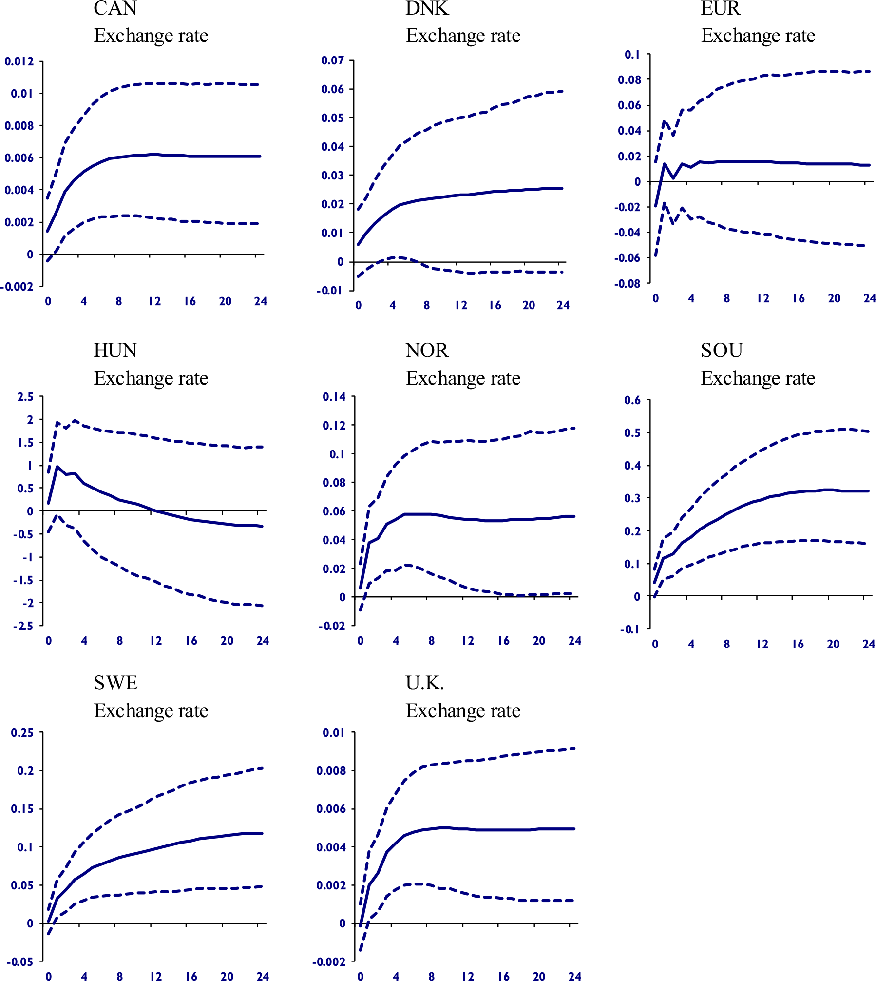
We found that the temperature anomaly shock triggers depreciations in domestic currencies (Figure 1). In some economies, this effect lasted for the entire shock (Canada, Norway, South Africa), while in others, it was short-lived (Denmark, Sweden, and the U.K.). The Eurozone and Hungary showed statistically nonsignificant responses.
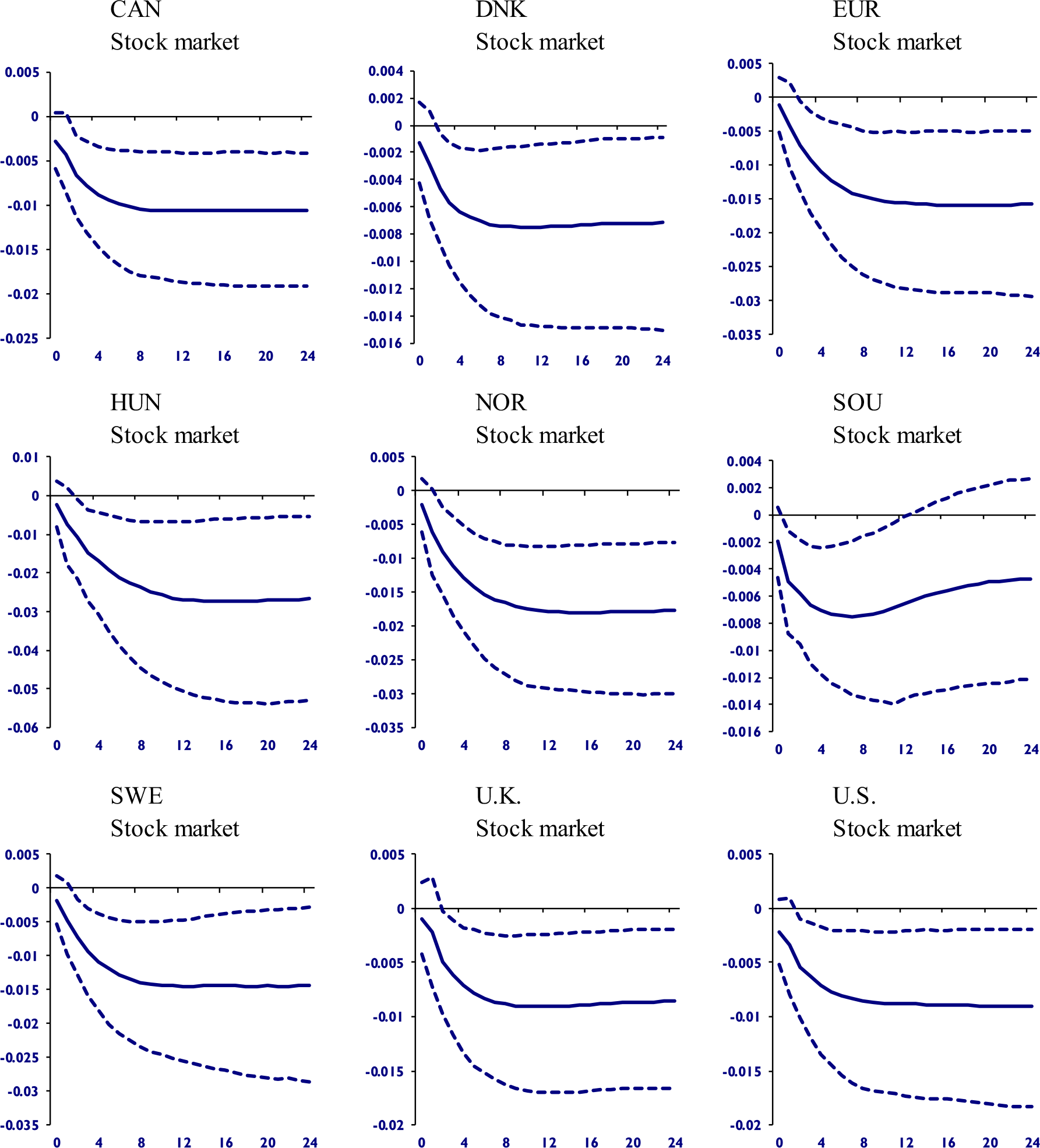
Figure 2 shows that all domestic stock markets react to the shock, presenting declining values. Similar to the responses of exchange rates, we detect two patterns: lasting and short-lived effects. Hence, our estimates indicate that the temperature anomaly provokes persistent and widespread fluctuations in the exchange and stock markets. These fluctuations suggest that increasing global temperatures correspond to higher stress levels in financial markets.
As mentioned earlier, the GIRF does not identify shocks, so we cannot establish causal relationships in the movements of the variables. However, we can hypothesize how financial markets respond to the temperature shock. One hypothesis is that climate change negatively affects the economies (Nordhaus, Reference Nordhaus2019; Ortiz-Bobea et al. Reference Ortiz-Bobea, Ault, Carrillo, Chambers and Lobell2021). Consequently, as financial markets price the future, stock markets may fall due to the worsening of expectations. Capital outflows may have weakened domestic currencies, explaining the depreciations in Figure 1. Lee et al. (Reference Lee, Mark, Nauerz, Rawls and Wei2022) investigated the impact of increasing temperature anomalies on the exchange rates of 76 economies. The authors concluded that the effect of the temperature is heterogeneous. Figure 1 shows the generalized depreciation of domestic currencies.
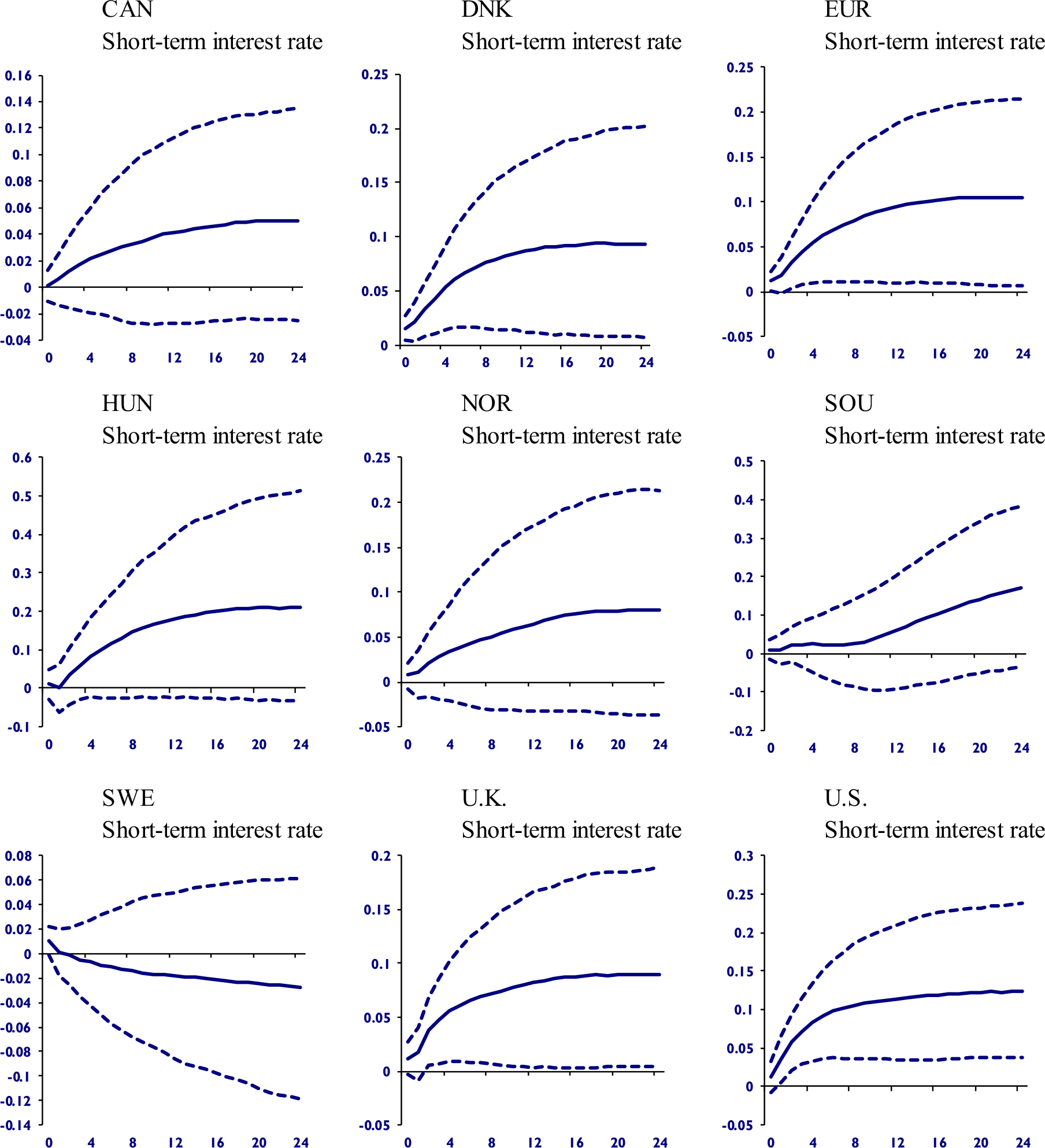
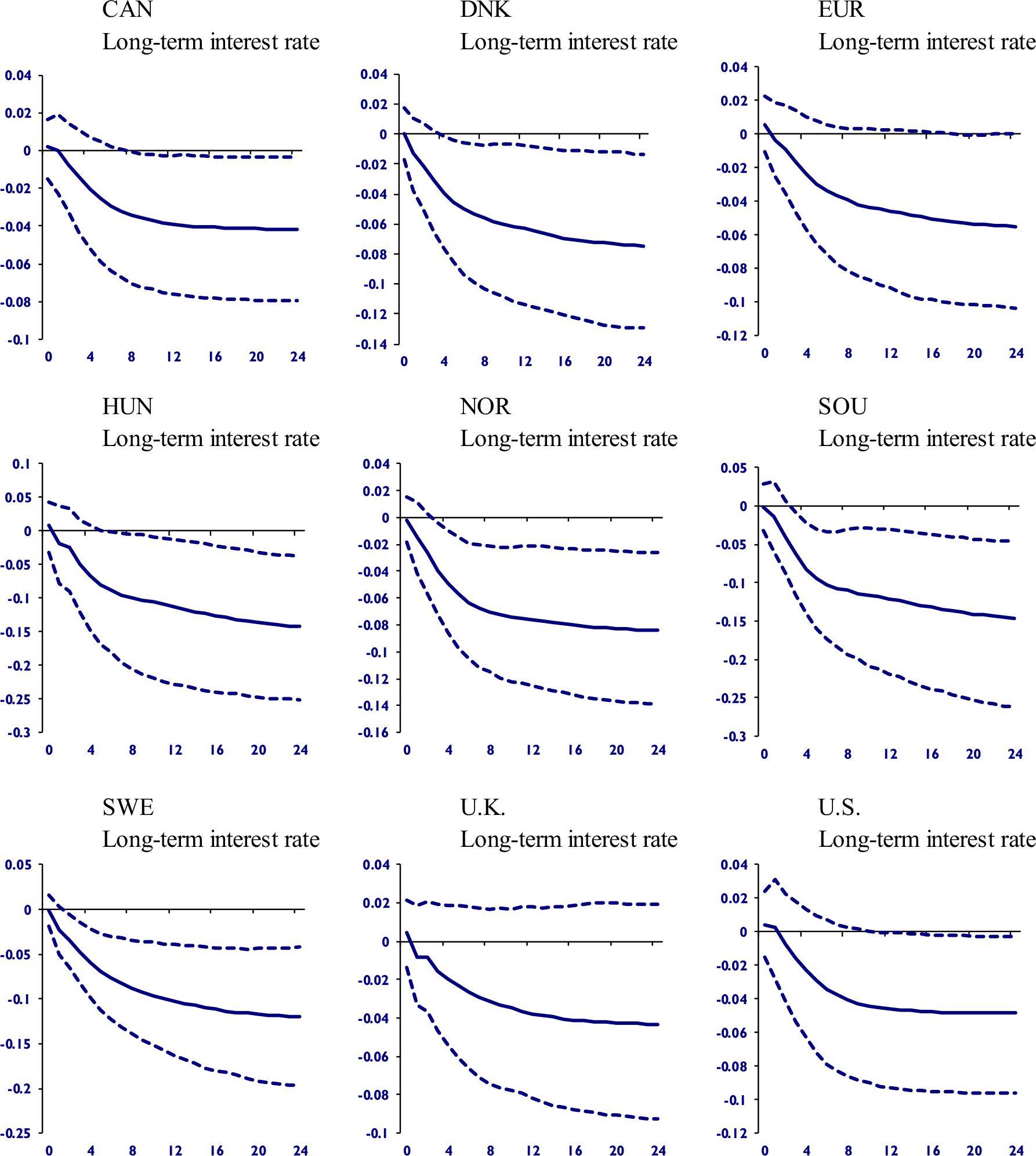
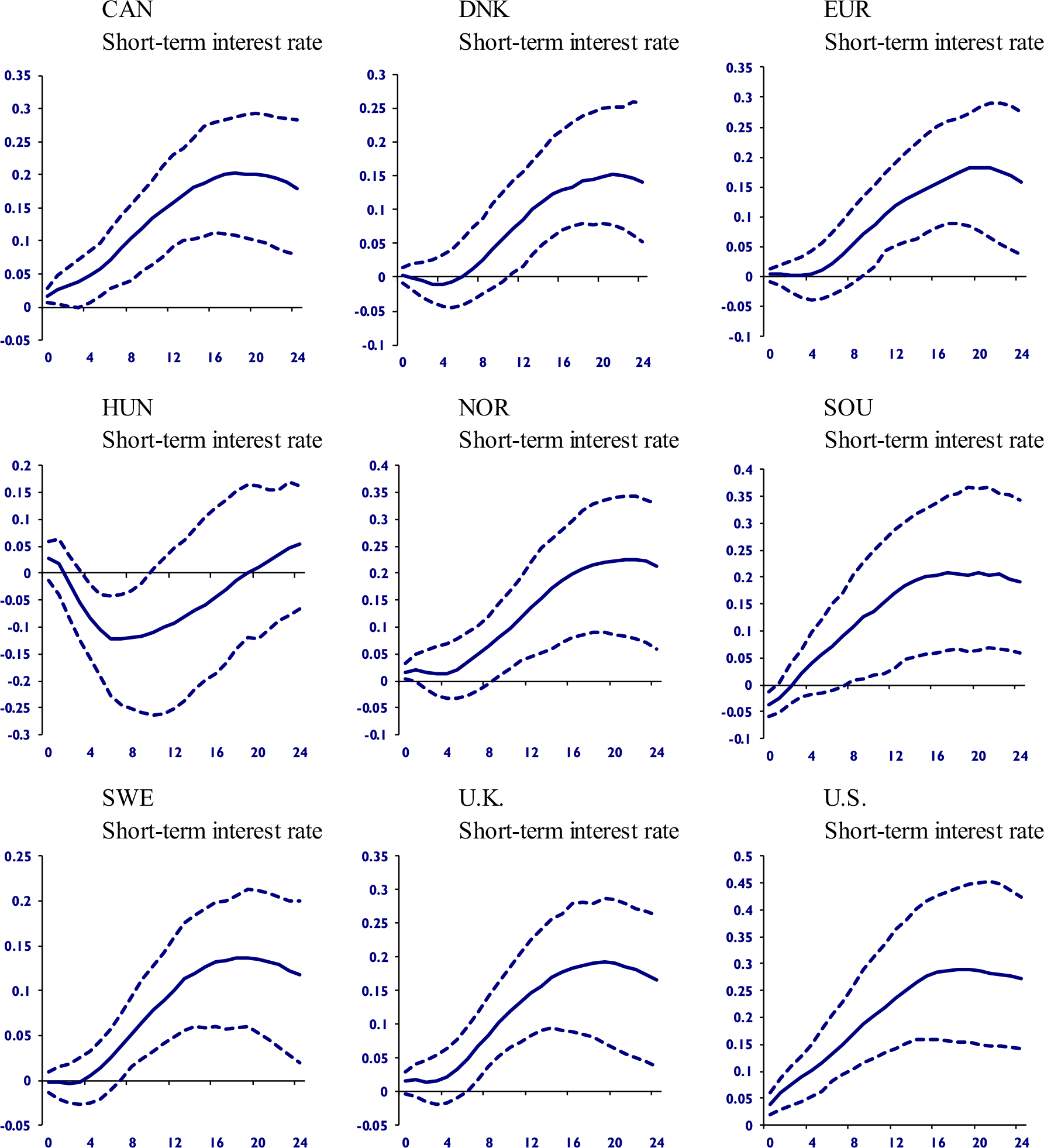
With the exception of Denmark and the U.S., almost all short-term credit markets showed no response to the shock, as depicted in Figure 3. In both economies, short-term interest rates increased. In Figure 4, long-term interest rates fell in five economies (Canada, Hungary, Norway, South Africa, and Sweden). These declining values may be associated with the financial market’s perception of future challenges due to climate change. Additionally, declines in long-term interest rates were observed, which are often considered indicators of impending recessions (Rosenberg and Maurer, Reference Rosenberg and Maurer2008; Engstrom and Sharpe, Reference Engstrom and Sharpe2019).
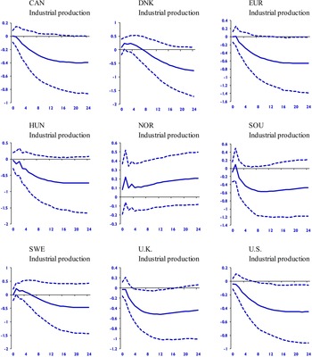
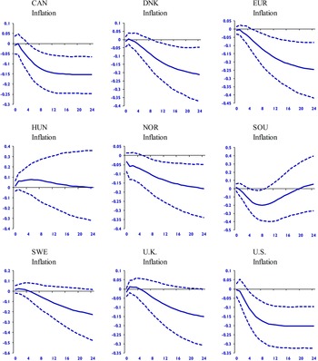
Figure 5 provides the responses of industrial production. Figures 1, 2, 3 and 4 suggest that financial markets exhibit responses to increasing temperature anomalies. Next, we examine whether these fluctuations affect production. The estimates show that production decreases in Canada, the Eurozone, the U.K., and the U.S. Therefore, these findings support the hypothesis that increasing temperature anomalies are linked to declining production. Furthermore, Figures 1, 2, 3, 4 and 5 raise the possibility that financial market mechanisms transmit the temperature anomaly shock, a hypothesis we explore in more detail in the next section. Figure 6 illustrates that prices decrease in most economies. This decline serves as another signal of a global recession resulting from the negative consequences of the temperature anomaly shock.
GIRF of temperature anomaly shock and responses of industrial production.

GIRF of temperature anomaly shock and responses of inflation.

Andrikopoulos et al. (Reference Andrikopoulos, Wang and Zheng2019) found limited evidence of the impact of weather anomalies on the currency markets of London and New York. Figure 1 challenges this finding by showing the generalized depreciation of domestic currencies relative to the U.S. dollar. Regarding stock markets, Cao and Wei (Reference Cao and Wei2005), Floros (Reference Floros2008), and Peillex et al. (Reference Peillex, El Ouadghiri, Gomes and Jaballah2021) documented that the value of stocks decreases due to higher temperature anomalies. Figure 2 reinforces this conclusion by showing the decline of international stock markets.
Hao et al. (Reference Hao, Chen and Chen2023) and Yang and Hamori (Reference Yang and Hamori2023) found that climate change affects credit markets, impacting loans and sovereign risk, while Mukherjee and Ouattara (Reference Mukherjee and Ouattara2021) argued that temperature shocks put pressure on central banks to implement contractionary monetary policies. Figures 3 and 4 complement and extend these studies. Both short- and long-term interest rates are sensitive to temperature anomalies, confirming the prediction by Mukherjee and Ouattara (Reference Mukherjee and Ouattara2021) that central banks may have to respond to temperature shocks. Figure 3 shows that the proxy for monetary policy (short-term interest rate) responds to temperature anomalies in Denmark and the U.S. Figure 4 shows that long-term interest rates, like loans and sovereign risk, are vulnerable to temperature anomalies.
Henseler and Schumacher (Reference Henseler and Schumacher2019), Holtermann (Reference Holtermann2020), and Aslan et al. (Reference Aslan, Altinoz and Polat2024) demonstrated that production is sensitive to temperature and weather anomalies. In particular, Aslan et al. (Reference Aslan, Altinoz and Polat2024) found that temperature anomalies negatively impact European production. We extend this result to other regions. Finally, contrary to Mukherjee and Ouattara (Reference Mukherjee and Ouattara2021), who found inflationary pressure due to temperature shocks, Figure 6 illustrates a deflationary process in economies.
Thus, most of the results in this section align with the literature. The main exception is inflation, which decreases. The recession caused by temperature anomalies may have reduced prices, a hypothesis supported by the decline in stock markets and long-term interest rates.
On the other hand, a decline in production, reflecting a decrease in aggregate supply, could lead to higher prices, a phenomenon known as stagflation. Although we do not conduct a causality analysis, we hypothesize that the decline in inflation may be driven by other factors influencing the adjustment to the shock. For instance, a drop in the stock market creates a wealth effect, reducing consumers’ purchasing power. Additionally, the uncertainty caused by the temperature anomaly shock – reflected in the depreciation of domestic currencies – may lead consumers and investors to postpone spending, weakening aggregate demand. Consequently, even with a decline in aggregate supply, weaker aggregate demand could explain the fall in inflation.
Regarding financial markets, stock markets may price in the negative consequences of temperature anomalies, much like they do with other weather-related disruptions such as floods, heavy precipitation, and heat waves, which hinder production. As a result, expectations of these future events could be reflected in stock prices, leading to market declines due to anticipated lower profits. In response to falling stock prices, investors may withdraw their capital and shift to safer assets, such as U.S. government bonds. This capital outflow could contribute to the depreciation of domestic currencies—a common occurrence during crises and periods of uncertainty when investors seek lower-risk financial positions.
The decline in long-term interest rates may signal, similar to stock markets, a potential future recession. Movements in stock and currency markets further reinforce this possibility. The increase in short-term interest rates, often a proxy for monetary policy, could suggest that central banks are attempting to curb capital outflows and mitigate domestic currency depreciation. However, our results do not confirm this connection.
Finally, the interaction among these markets—particularly the decline in stock markets—helps explain the indirect impact of temperature anomalies on production. In this framework, financial markets serve as a transmission channel for temperature anomaly shocks. However, as demonstrated in the next section, temperature anomalies can also have a direct impact on production, much like other weather anomalies, by damaging infrastructure, disrupting economic activity, and worsening conditions for production, particularly in agriculture.
6.2 Transmission channels
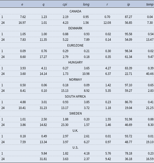
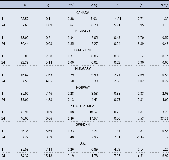
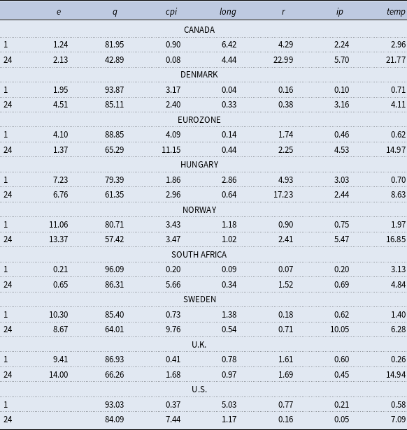
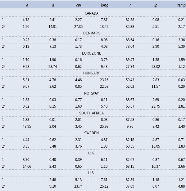
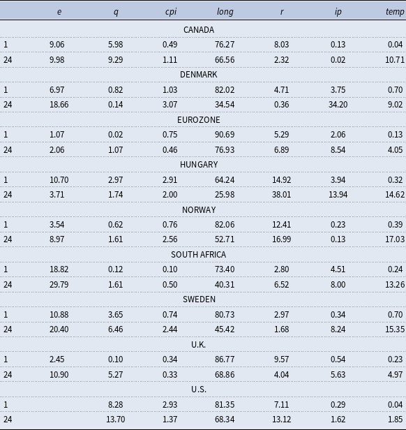
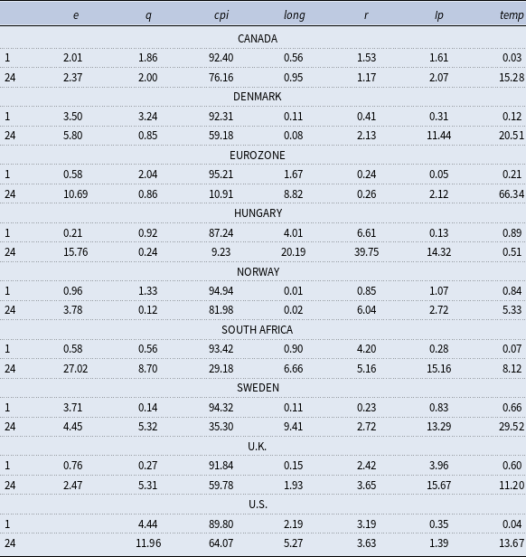
We use the GFEVD to evaluate the direct and indirect influence of temperature anomalies on the economies. Tables 2, 3, 4, 5, 6, and 7 present the decomposition of future values for production, exchange rates, stock markets, short- and long-term credit markets, and inflation, respectively. This decomposition is divided into two blocs. The first shows the domestic variables (e, q, cpi, long, r, ip). The second bloc presents the temperature anomaly. Therefore, comparing the importance of domestic factors to the influence of temperature allows us to better understand the fluctuations of these variables. We normalized each table to a sum of 100% in each row to facilitate comparison across variables.
GFEVD of industrial production to domestic factors and temperature anomalies

GFEVD of exchange rate to domestic factors and temperature anomalies

Note: The U.S. does not appear in this table because of the reasons discussed in Section 3.
GFEVD of stock market to domestic factors and temperature anomalies

GFEVD of short-term interest rates to domestic factors and temperature anomalies

GFEVD of long-term interest rates to domestic factors and temperature anomalies

GFEVD of inflation to domestic factors and temperature anomalies

The reading of the tables is as follows: in Table 2, for Canada, in the first period, exchange rates affect industrial production by 7%, the stock market affects production by 1%, inflation affects production by 2%, long-term interest rates have a 0.9% influence on production, short-term interest rates influence production to the extent of 0.7%, and industrial production affects itself by 87%. These are the domestic factors affecting industrial production. The last column shows that the temperature anomaly explains almost 0% of the industrial production fluctuation. However, in the last period, the temperature anomaly affects industrial production by 7%.
Another piece of information from Table 2 is that, in the last period for Canada, all financial markets affected industrial production to varying extents. Based on the magnitude of the estimates, the exchange and long-term credit markets are the principal financial markets contributing to changes in industrial production. The relevance of this observation is that these markets are potential transmission channels of the temperature anomaly shocks. If we observe that temperature anomalies affect financial markets, we can return to Table 2 and conclude that, indirectly, temperature anomaly affects production by causing changes in the financial markets. That is the strategy we follow to detect transmission channels in Tables 2, 3, 4, 5, 6, and 7.
In summary, Table 2 shows that temperature anomalies affect industrial production in all economies. Except in Norway, the magnitude of temperature anomaly effects in the last period varied between 7% (Canada) and 40% (Hungary). This result highlights a direct link between temperature anomalies and industrial production. Regarding the potential mechanisms of transmission, we found that financial markets affect industrial production in all economies, with considerable heterogeneity. For example, in the last period, the currency markets are the principal financial markets affecting production in Canada, the stock markets in Denmark, the Eurozone, Hungary, South Africa, Sweden, the U.K., and the U.S., and the long-term credit market in Norway. Consequently, our estimates suggest that the stock markets serve as critical conduits for the effect of temperature anomalies on production in most economies. Although the short-term credit markets are not the principal financial markets in any economy, they have significant values, such as in Canada (12%) and the U.S. (9%).
In Table 3, the findings indicated that the temperature anomaly has a significant impact on Canadian and South African currency fluctuations (and with a minor effect observed in the U.S. and Norway). The influence of temperature anomalies is more pervasive and persistent in the stock markets (Table 4). In the last period, temperature anomalies explain 4%-21% of the fluctuation in the stock markets. Notably, Canada, the Eurozone, Norway, and the U.K., where the temperature anomaly causes at least 15% of domestic fluctuations. Therefore, given the findings from Table 2 showing that these financial markets affect industrial production, Tables 3 and 4 allow us to conclude that, indirectly, temperature anomalies affect industrial production by causing changes in the exchange and the stock markets.
Temperature anomaly induces minor changes in the short-term credit market (Table 5). Conversely, Table 6 shows that the long-term credit markets exhibit a significant influence of the temperature anomaly. The relevance of temperature anomaly is approximately 15% in Hungary, Norway, South Africa, and Sweden. These findings demonstrate that credit markets serve as another transmission channel for temperature anomaly shocks. Therefore, our estimates confirm the existence of four transmission channels for temperature anomaly shocks.
In summary, Table 7 shows that temperature anomalies affect inflation in all economies. Certain economies demonstrate greater vulnerability to climate change, such as Canada (15% in the last period), Denmark (20%), the Eurozone (66%), and Sweden (29%). These findings suggest that climate change may impact consumers’ purchasing power in addition to the fluctuations depicted in Tables 2, 3, 4, 5 , and 6. Finally, Sections 6.1 and 6.2 demonstrate that temperature anomalies have direct and indirect effects on industrial production, with financial markets serving as transmission channels for the shock. The rest of the empirical section implements robustness checks.
6.3 Changing bilateral trade (1999–2001 and 2020–2022)
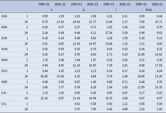
Until now, our model has relied on bilateral trade from the years 2020-2022. To assess the impact of bilateral trade on the findings in Sections 6.1 and 6.2, we propose varying the years of bilateral trade. Given our study’s timeline from January 1999 to January 2023, we incorporate bilateral trade from the earlier years, specifically 1999-2001. This analysis aims to ascertain the relevance of trade integration in understanding the propagation of temperature anomaly shocks on financial markets. Consequently, Table A6, in the Appendix, presents estimates for the four financial markets, using the same model but with adjustments to the average bilateral trade. The values in columns 2020–2022 mirror those in previous tables. We introduce the column 1999–2001 to evaluate the impact of trade integration.
In Table A6, we present the four financial markets across two columns. The 2020–2022 column replicates the temperature anomaly values from the previous tables. Essentially, we computed the influence of domestic factors and temperature anomalies on the fluctuations of a specific domestic financial market. However, in Table A6, we only present the influence of temperature anomalies. The 1999–2001 column demonstrates the impact of temperature anomalies on the financial markets (note that we calculated both domestic factors and temperature anomalies, but due to space constraints, we report only the latter).
According to Table A6, the explanatory power of temperature anomalies decreased in explaining fluctuations in short-term credit markets (r) from 1999–2001 to 2020–2022, except in South Africa. In all economies, the influence of temperature anomalies was higher in 1999–2001 than in 2020–2022. Conversely, regarding long-term interest rates (long), temperature anomalies gained explanatory power over the years. However, for exchange rates (e) and stock markets (q), there is no clear pattern of change based on bilateral trade.
Another finding from Table A6 is that the relative importance of temperature anomalies does not appear to depend critically on bilateral trade. Despite the changes identified between short- and long-term credit markets, the impact of temperature anomalies on each financial market remains relatively consistent. For instance, in South Africa, we observed that temperature anomalies notably influence the domestic currency. However, even with changes in bilateral trade, this influence remained significant in 1999–2001.
6.4 Time-varying weights
Another robustness exercise involves considering time-varying bilateral trade. In Sections 6.1 and 6.2, we used fixed weights to construct the international scenario (foreign variables) and solve the model. However, in Section 6.3, we altered the bilateral trade years to 1999–2001. Here, we analyze bilateral trade across all years, employing moving averages to construct the foreign variables. This approach allows us to account for changes in bilateral trade over time. Figures A1, A2, A3, and A4, in the appendix, depict the results, reproducing Figures 2, 3, 4, and 5 but using time-varying bilateral trade. We excluded the last observation (2023M1), as the bilateral trade data is available only until 2022. Consequently, our analysis spans from 1999M1 to 2022M12. We focus solely on financial market responses, aligning with our objective of evaluating the sensitivity of transmission channels to structural changes and spatial considerations.
Observing Figures A1, A2, A3, and A4, we note that the main results remain unchanged. Figure A1 illustrates the depreciation of domestic currencies, Figure A2 presents generalized declines in stock markets, Figure A3 displays increases in short-term interest rates, and Figure A4 shows that long-term interest rates decline due to the temperature anomaly shock. Although the results are quantitatively similar to those in Section 6.1, we made qualitative improvements.
Regarding the credit markets, in Figure 3, only in Denmark and the U.S. did short-term interest rates increase in response to the shock. However, in Figure A3, we observed this movement in four economies (Denmark, the Eurozone, the U.K., and the U.S.). Another distinction can be made by comparing Figures 4 and A4. In Figure 4, five economies showed declining interest rates, whereas in Figure A4, except for the U.K., all economies experienced declining long-term interest rates.
Figures A1, A2, A3, and A4 corroborate our estimations using fixed bilateral trade. The results remain consistent with those in Figures 1, 2, 3, and 4, regardless of how bilateral trade is treated. Although we do not depict this due to space constraints, the model utilizing fixed weights for the years 1999-2001 also exhibited similar responses (results are available upon request).
6.5 Oil and agricultural prices
Global prices may affect financial markets. Among the principal global prices are oil prices and agricultural prices. We test our results by including these variables in the model. We collected oil prices from FRED, using the West Texas Intermediate (WTI) oil prices, and seasonally adjusted this time series. Agricultural prices were sourced from the Primary Commodity Prices of the IMF. We use the agriculture price index, which includes agricultural raw material prices, and also seasonally adjusted this time series. Both variables were included as domestic variables in the U.S. model and as foreign variables for the rest of the countries. Figure A5, in the appendix, presents the GIRF of a temperature anomaly shock.
The responses of the financial markets are similar to those we portrayed in the paper: domestic currencies depreciate against the dollar, stock markets decline, short-term interest rates are less responsive, and long-term interest rates decrease. This last result represents a qualitative improvement. For example, in Figure 4, most long-term interest rates decreased, but they were statistically nonsignificant. In Figure A5, all long-term rates decreased in response to the temperature anomaly shock.
6.6 Alternative periods
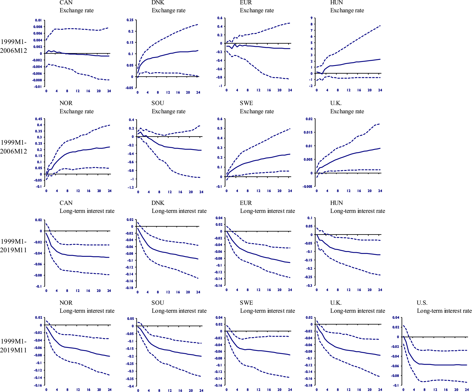
We test our results using two alternative periods. The first excludes the 2007-2008 financial crisis, which provoked strong fluctuations in the financial markets. Thus, the first period we evaluate is from January 1999 to December 2006. The second period excludes the COVID-19 pandemic, which, similar to the 2007-2008 financial crisis, caused fluctuations in financial markets. We exclude this pandemic by analyzing the period between January 1999 and November 2019. Both episodes could affect our results due to structural breaks in the time series. Figure A6, in the appendix, presents the results of a temperature anomaly shock in both periods.
Due to space constraints, we do not present the reactions of all financial markets in Figure A6. Instead, we chose to show only the financial markets with the most statistically significant responses. The first period (1999M1–2006M12) shows that exchange rates increased in response to the shock in most economies. In contrast, in the second period (1999M1–2019M11), long-term interest rates decreased in response to the temperature shock in all economies. This division suggests that before the 2007-2008 financial crisis, the most sensitive financial market to temperature anomaly shocks was the currency market, whereas, right before the pandemic, it was the long-term credit market. One drawback that could negatively affect our results is the loss of observations due to the reduction in the timeframe. However, the main results remained consistent.
6.7 Carbon emissions
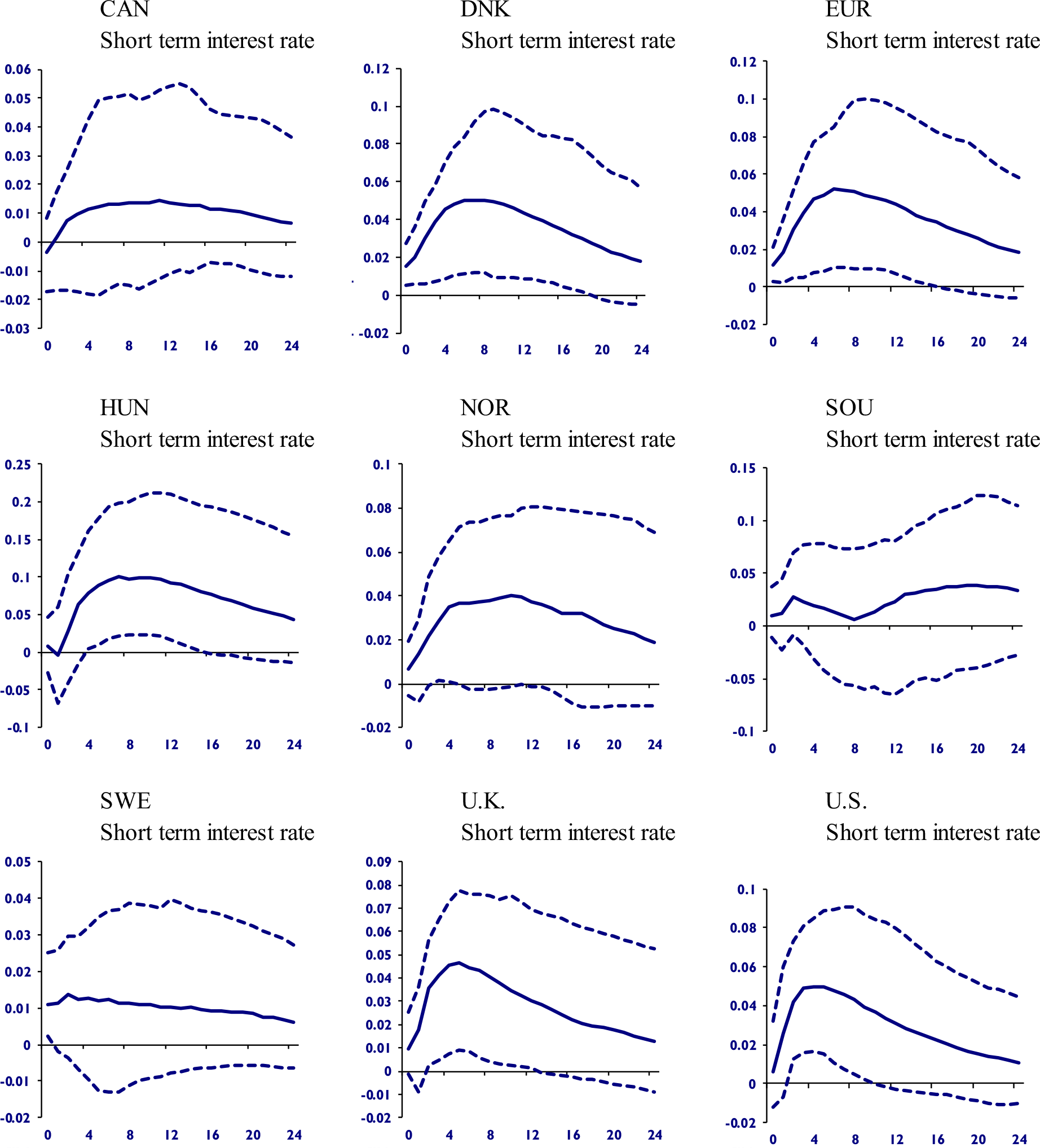
We test another proxy for temperature anomaly using carbon emissions data from the World Bank. Since higher temperatures correlate with higher carbon emissions, this serves as an alternative proxy. We applied the Denton procedure to convert the frequency of carbon emissions from annual to monthly. Additionally, we used log differences in this time series. We included this variable as a domestic variable in the U.S. model and as a foreign variable in the models of other economies. Figure A7, in the appendix, presents the GIRF of a carbon emission shock.
In Figure A7, we present only the responses of short-term interest rates, as this was the principal qualitative improvement from this new configuration. While in Figure 3 the short-term interest rates had statistically nonsignificant values, we now find that all economies (except Hungary) respond with higher short-term interest rates to the carbon emission shock.
6.8 Dominant model
Until now, we have used the temperature anomaly as a domestic variable in the U.S. model. The U.S. is an internationally relevant economy, influencing national business cycles and affecting several financial markets worldwide. Additionally, in our sample of 20 countries, the U.S. economy represents 47% of the sample GDP for the years 2019–2021. In other words, the U.S. may be more influential in causing changes in temperature anomalies than other countries. However, since the temperature anomaly is a global variable, it can be argued that its inclusion should be in the dominant unit model.
In the GVAR, the dominant unit model is an additional regression with global variables. By using this configuration, the global variable (temperature anomaly) is included in this regression while being treated as a foreign variable in the rest of the countries (including the U.S.). Figure A8, in the appendix, presents a temperature anomaly shock in the dominant unit model configuration.
Due to space constraints, we present the main difference from the previous results. The short-term interest rates increased for most economies, whereas in the previous results, this variable was statistically nonsignificant. Although we do not present them here, exchange rates, long-term interest rates, and stock markets reacted as observed in the paper. Thus, using the temperature anomaly as a domestic variable in the U.S. or as a global variable in the dominant unit model does not affect our main results.
6.9 Exchange rte in the U.S. model
Our final econometric test includes an exchange rate variable in the U.S. model as a domestic variable. We collected the Real Broad Effective Exchange Rate (RBEER), Index 2020 = 100, from the FRED. This index is a weighted average of bilateral exchange rates adjusted by relative consumer prices (we seasonally adjusted it). A notable difference compared to the exchange rates used in this paper is the interpretation of movements. When the RBEER increases, the U.S. dollar appreciates relative to other currencies. Conversely, when the RBEER decreases, it indicates a depreciation of the U.S. dollar. The RBEER provides a general view of the U.S. dollar relative to other currencies. We included the RBEER as a domestic variable in the U.S. model and excluded the foreign exchange rate. Figure A9, in the appendix, presents the responses of the exchange rates to a temperature anomaly shock.
As observed earlier, domestic currencies depreciate in response to the shock in most economies (Canada, Norway, South Africa, Sweden, and the U.K.). Now we have evidence that the U.S. currency appreciates after the temperature shock, with the RBEER increasing over time. Thus, the inclusion of an exchange rate in the U.S. model does not change the result that domestic currencies depreciate relative to the U.S. dollar.
7. Conclusion
7.1 Contributions
We analyzed the impact of temperature anomalies on 20 economies and observed that industrial production reacts negatively, with financial markets serving as conduits for transmitting the shock. Our robustness checks indicated that the configuration of bilateral trade is not pivotal for these results.
We contribute to the literature by: i) providing an economic rationale for the impact of temperature anomalies on a system of open economies, ii) treating temperature anomalies as an externality, thus capturing one of the principal characteristics of climate change, and iii) portraying direct and indirect linkages between climate change and fluctuations in production, highlighting heterogeneities, and capturing spillover effects.
7.2 Theoretical implications
If we are not mistaken, this is the first study to connect temperature anomalies to financial markets and production. The rationale proposed by the theoretical model, in which climate change-induced fluctuations in financial markets affect production, was confirmed by the empirical model. Thus, this study demonstrates that financial markets serve as channels for understanding how temperature anomalies impact the goods market. We propose that this occurs through at least four financial markets: currency markets, foreign markets, short-term credit markets, and long-term credit markets.
7.3 Limitations and future research
One limitation of our study is the absence of noneconomic variables to elucidate the diffusion of temperature anomaly shocks on economies. Variables such as environmental regulation, local weather risk (or another geographical variable), and the consumption of renewable energy could potentially aid in explaining how economies react to climate change. Future research could incorporate these channels and assess how they interact with temperature anomalies. Another avenue is the adoption of microeconomic studies to scrutinize the relationships between financial markets, climate change, and production. While we provided a macroeconomic perspective, causality analyses are encouraged to further explore transmission channels. Finally, there can be nonlinear effects of temperature anomalies. We used a linear model. Future research could explore the nonlinear effects of temperature anomalies on economies.
7.4 Policy implications
As a policy recommendation, governments and policymakers should adopt monetary and fiscal policies to mitigate and alleviate the consequences of climate change. Our results indicate that higher temperature anomalies correlate with recessions. Accommodative policies can help mitigate the negative impact of climate change: central banks could reduce interest rates, and governments could increase fiscal spending to counterbalance the recessionary impact of temperature anomalies.
We found that domestic currencies depreciate and stock markets lose value in response to temperature anomalies. These fluctuations can lead to reduced purchasing power and a decline in wealth, potentially exacerbating the severity of the temperature anomaly shock. Implementing fiscal transfers for vulnerable individuals can help shield them from this adversity. Naturally, the potential increase in the public deficit should be counterbalanced once the shock has faded. One approach is for governments, knowing that temperature anomalies may require higher fiscal spending, to create fiscal funds for use in these situations. These funds could finance fiscal spending while maintaining fiscal sustainability. The goal is to avoid increasing public debt and keep the macroeconomic environment stable.
Given the potential negative impact of higher temperatures on production (including agricultural production, although we did not explore this point), governments could create and raise public funds explicitly targeted to mitigate the damage in this area. These funds could be invested in low-risk liquid assets, such as public bonds, and used when natural disasters occur, such as floods, droughts, and excessive rains. Ideally, this fund would be self-sustainable, avoiding fiscal pressure on the public budget. The policies could include subsidized credit and tax breaks for producers affected by and more vulnerable to temperature anomalies. Like the fiscal policies mentioned above, these policies should be reversed once the shock fades, given the transitory nature of the shock.
Governments should manage their fiscal accounts carefully, as climate change can lead to higher public spending. Structural reforms, such as administrative and pension reforms, particularly in the public sector, could help reduce spending and increase revenues. These reforms could alleviate the public budget by reducing spending, thereby creating the possibility of reducing the public debt-to-GDP ratio and the subsequent interest payments on this debt. Ideally, governments would present a declining debt-to-GDP ratio, fiscal surpluses, and resources to boost funds targeted at mitigating the negative consequences of temperature anomalies.
Finally, the fluctuations we detected in the empirical part indicate that temperature anomalies affect financial markets. Policymakers should allow financial markets to respond to these events instead of imposing controls, such as capital controls. These fluctuations help portray and absorb the shock. Financial markets transmit information to individuals and companies. On the other hand, as we argued, governments and policymakers could help the situation through public and fiscal programs targeted at damaged areas and groups.
7.4 Practical implications
The worsening of climate change and its negative consequences may put pressure on countries. In particular, as suggested by the results, widespread fluctuations in financial markets, production, and inflation could emerge, affecting business cycles. Furthermore, as our study indicates, the consequences of climate change can be interpreted as external shocks with global economic implications. The progression of climate change may pose new challenges for policymakers and the goal of short-term economic stability.
Competing interests
The authors report there are no competing interests to declare.
Funding statement
This research did not receive any specific grants from public, commercial, or nonprofit agencies.
Data availability statement
The data supporting the findings of this study are available from the corresponding author upon request.
Appendix
Figures A1, A2, A3, A4, A5, A6, A7, A8, A9 and Tables A1, A2, A3, A4, A5, A6.
GIRF of temperature anomaly shock and responses of exchange rates (time-varying bilateral trade model, 1999M1-2022M12).

GIRF of temperature anomaly shock and responses of stock markets (time-varying bilateral trade model, 1999M1–2022M12).

GIRF of temperature anomaly shock and responses of short-term interest rates (time-varying bilateral trade model, 1999M1–2022M12).

GIRF of temperature anomaly shock and responses of long-term interest rates (time-varying bilateral trade model, 1999M1–2022M12).

Model with oil and agricultural prices (GIRF of a temperature anomaly shock).

Alternative periods (1999M1–2006M12 and 19991–2019M11)—GIRF of a temperature anomaly shock.

GIRF of a carbon emission shock and responses of short-term interest rates.

Dominant Unit Model—GIRF of a temperature shock.

Model with RBEER in the U.S. model (GIRF of a temperature anomaly shock)

Descriptive statistics

Unit root test (weighted symmetric) for domestic variables at 5% significance level

Unit root test (weighted symmetric) for foreign and global variables at 5% significance level

VARXs order and cointegrating relationships

Test for weak exogeneity at 5% significance level

GFEVD of domestic variables to temperature anomaly in 1999–2001 and 2020–2022