2 Theory

The fully nonlinear equations for two-dimensional motion in the $y$ – $z$ plane of inviscid, incompressible, Boussinesq fluid on the $f$ plane with arbitrary stratification are given in terms of the spanwise vorticity, ${\it\zeta}=w_{y}-v_{z}=-{\rm\nabla}^{2}{\it\psi}$ , and buoyancy, $b=-g{\it\rho}/{\it\rho}_{0}$ (in which $g$ is gravity and ${\it\rho}_{0}$ is a characteristic density):

and

in which the subscripts denote derivatives. The horizontal and vertical velocities are given by derivatives of the streamfunction ${\it\psi}$ by $v={\it\psi}_{z}$ and $w=-{\it\psi}_{y}$ . The spanwise velocity, $u$ , is given by the $x$ -momentum equation:

Being on the $f$ -plane, the Coriolis parameter, $f$ , is taken to be constant. The squared buoyancy frequency, defined in terms of the background density gradient by $N^{2}=-(g/{\it\rho}_{0})\,\text{d}\bar{{\it\rho}}/\text{d}z$ , is generally a function of $z$ , being constant only for the case of uniformly stratified fluid.

For small-amplitude disturbances, the nonlinear terms on the right-hand sides of (2.1) and (2.2) are negligible. The resulting coupled linear partial differential equations can be Fourier transformed in horizontal space and time so that a particular mode can be written

in which ‘ $\text{c.c.}$ ’ denotes the complex conjugate, $\ell$ is the horizontal wavenumber (in the $y$ -direction) and ${\it\omega}$ is the frequency of the particular vertical mode in question. The vertical structure of the streamfunction, $\hat{{\it\psi}}$ , and the corresponding frequency are found from the solution of the eigenvalue problem

The vertical structure of the buoyancy is given in terms of $\hat{{\it\psi}}$ from the linear terms in (2.2):

For conceptual convenience, the (possibly complex) amplitude ${\mathcal{A}}$ is set so that $\hat{{\it\psi}}$ (hence also $\hat{b}$ ) is a real-valued function with maximum value, $\Vert \hat{{\it\psi}}\Vert$ , being order unity.

Of course, if $N=N_{0}$ is constant, then analytic solutions of (2.6) are readily found: $\hat{{\it\psi}}=\sin (k_{m}z)$ . For a domain of depth $H$ , the vertical wavenumber holds discrete values $k_{m}=m{\rm\pi}/H$ for positive integers, $m$ . The corresponding dispersion relation is

In general, if $N$ varies with $z$ , then $\hat{{\it\psi}}$ and ${\it\omega}(\ell ,k_{m})$ must be determined numerically as an eigenvalue problem for each mode number, $m$ .

Now consider the self-interaction of a single mode through the nonlinear terms in (2.1) and (2.2). Using (2.6) to recast second derivatives of $\hat{{\it\psi}}$ in terms of $\hat{{\it\psi}}$ and simplifying, the nonlinear terms in the vorticity equation become

Using (2.7), the nonlinear terms in the buoyancy equation become

The forcing terms have similar structure to the right-most expressions of Diamessis et al. (Reference Diamessis, Wunsch, Delwiche and Richter2014, equations (7) and (8)), though those equations ignore rotation and assume steady state resulting from an incident vertically propagating wave beam transferring energy to superharmonics. The right-hand sides of (2.9) and (2.10) express the contribution of the advective terms upon the time rate of change of superharmonic vorticity and buoyancy, respectively.

Crucially, both terms are multiplied by the $z$ -derivative of $N^{2}$ . If the stratification is uniform, both nonlinear terms vanish. This is just the well-known result that monochromatic internal waves in uniformly stratified fluid are an exact solution of the fully nonlinear equations of motion. This is true whether the waves are unbounded or confined as modes. (For uniform stratification, the advection terms of the momentum equations do not vanish upon substituting the sinusoidal structure of the vertical modes in a channel. But from the diagnostic pressure equation (computed from the divergence of the momentum equations), it is found that the order amplitude-squared pressure resulting from the advection terms has a gradient force that exactly cancels the forcing from the advection terms. Working with vorticity, rather than momentum and pressure, makes it clear that even vertically confined modes are an exact solution of the fully nonlinear equations in uniform stratification.) In the examination of PSI of modes in uniformly stratified fluid, it is necessary to suppose that (through noise) the given parent internal mode interacts with other small amplitude internal modes through the nonlinear terms (Bouruet-Aubertot, Sommeria & Staquet Reference Bouruet-Aubertot, Sommeria and Staquet1995). Depending upon their wavenumber and frequency, the small waves may grow at the expense of the parent mode.

By contrast, equations (2.9) and (2.10) show that disturbances in non-uniformly stratified fluid are created by the parent mode even in the absence of noise. But the vertical structure of the forcing does not correspond to that of any one mode. It is strongest where $N^{2}$ changes most rapidly with $z$ , whereas modes tend to have largest amplitude where $N$ itself is largest. The forcing has twice the horizontal wavenumber and frequency as the parent mode and so, at least initially, it gives rise to superharmonic disturbances with the same horizontal phase speed as the parent mode. This synchronization means that the amplitude of the disturbance initially grows linearly in time. Because the excited disturbance is a superposition of vertical modes having wavenumber $2\ell$ and because each vertical mode has a different frequency the disturbances are not expected to maintain the phase speed of the parent mode. In particular, smaller vertical scale modes have smaller frequency and so are expected to move with slower phase speed than that of the parent mode.

As an example, consider the dispersion relation for vertical modes in top-hat-like stratification for which the squared buoyancy frequency is

If $0<{\it\sigma}\ll D\equiv z_{+}-z_{-}$ , then $N^{2}\simeq N_{0}^{2}$ for $z_{-}<z<z_{+}$ and $N^{2}\simeq 0$ otherwise. Assuming the domain extends vertically from $-H$ to $0$ , the stratified layer is symmetrically positioned in the vertical domain if $\bar{z}\equiv (z_{+}+z_{-})/2=-H/2$ .

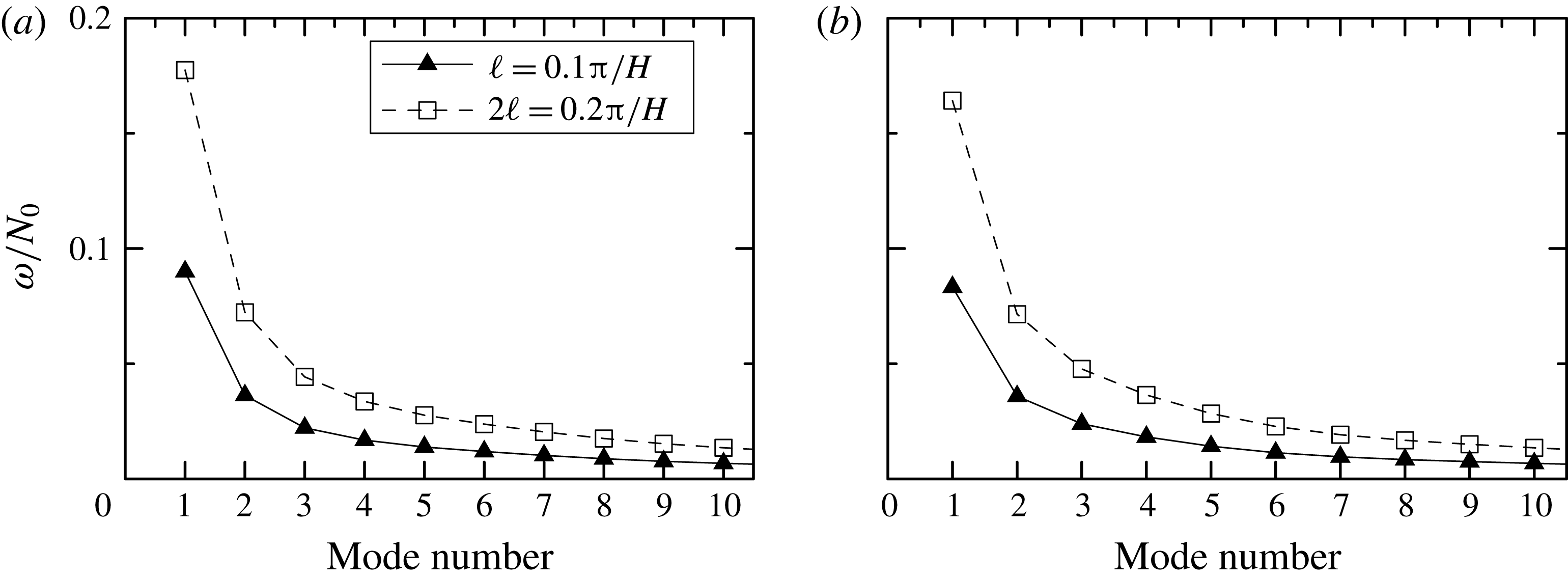
Figure 1 plots the dispersion relation for modes with horizontal wavenumber $\ell =0.1{\rm\pi}/H$ and $0.2{\rm\pi}/H$ . In the symmetric case with $\bar{z}=-0.5H$ , the mode-one parent wave with horizontal wavenumber $\ell _{0}=0.1{\rm\pi}/H$ has frequency ${\it\omega}_{0}\simeq 0.090N_{0}$ . According to (2.9), the forcing excites a disturbance with horizontal wavenumber $2\ell _{0}$ . However, in this symmetric case the vertical structure of the forcing is an odd function about the midpoint of the domain because the derivative of $N^{2}$ is equal and opposite on either flank of the stratified region. (This is shown explicitly in the corresponding simulation presented in the next section.) Therefore, the excited superharmonic disturbance should be dominated by a superposition of even modes. But the frequency of the mode-two wave with $\ell =2\ell _{0}$ is $0.072N_{0}$ , and the other even modes have still lower frequencies, all of which are well below the forcing frequency $2{\it\omega}_{0}\simeq 0.180N_{0}$ . Thus, the forcing resulting from the self-interaction of the parent mode does not directly excite a single superharmonic mode. Rather, it leads to the development of a superposition of modes that are superharmonic horizontally in space but with smaller temporal frequency than the parent mode. Simulations show that the consequent nonlinear evolution of the system gives rise to disturbances with frequencies both smaller and larger than the parent mode.

Figure 1.

Dispersion relation showing frequency as a function of mode number for modes in stratification given by (2.11) with ${\it\sigma}=0.016\,H$ , $D=0.5\,H$ and (a) $\bar{z}=-0.5H$ and (b) $\bar{z}=-0.35H$ . In each plot the dispersion relation is plotted for waves with horizontal wavenumber $\ell _{0}=0.1{\rm\pi}/H$ (solid line and solid triangles) and $\ell _{0}=0.2{\rm\pi}/H$ (dashed line and open squares), as indicated in the legend in (a).

If the stratification is asymmetric, the forcing may put more energy into the mode-one superharmonic. In particular, for the case with $\bar{z}=-0.35H$ , the frequency of the mode-one parent wave with $\ell _{0}=0.1{\rm\pi}/H$ is ${\it\omega}_{0}=0.083N_{0}$ . The mode-one superharmonic with $\ell =2\ell _{0}$ has frequency $0.164N_{0}$ , close to the forcing frequency of $2{\it\omega}_{0}$ . Hence, the forcing can result in reinforcement of a mode-one superharmonic though with some leftward drift as a consequence of the moderately lower frequency.

The latter behaviour is somewhat consistent with the examination of Diamessis et al. (Reference Diamessis, Wunsch, Delwiche and Richter2014), whose model assumed that an internal wave beam incident upon a localized region of enhanced stratification would excite superharmonics with exactly twice the horizontal wavenumber and frequency of the beam.

As the amplitude of the excited disturbance becomes sufficiently large it can interact nonlinearly with the parent mode itself. To gain some insight into such weakly nonlinear effects, consider the interaction between the parent mode and superharmonic disturbance that results in forcing at the horizontal wavenumber and frequency of the parent mode. At early times the vorticity field of the superharmonic, ${\it\zeta}_{2}$ , is assumed to have the structure of the forcing so that, from (2.9), ${\it\zeta}_{2}=\text{i}{\it\epsilon}\hat{{\it\zeta}}_{2}\exp [2\text{i}(\ell y-{\it\omega}t)]+\text{c.c.}$ , in which ${\it\epsilon}$ represents the real-valued amplitude after some small time and the complex number $\text{i}$ has been pulled out explicitly to emphasize that the superharmonic disturbance is $90^{\circ }$ out of phase with the parent mode. Given the vertical structure $\hat{{\it\zeta}}_{2}(z)$ , which is proportional to $\text{d}N^{2}/\text{d}z$ , one can go on to find the corresponding streamfunction, ${\it\psi}_{2}=\text{i}{\it\epsilon}\hat{{\it\psi}}_{2}\exp [2\text{i}(\ell y-{\it\omega}t)]+\text{c.c.}$ , in which $\hat{{\it\psi}}_{2}$ is the solution of

The corresponding horizontal and vertical velocity fields are $v_{2}=\text{i}{\it\epsilon}\hat{{\it\psi}}_{2}^{\prime }\exp [2\text{i}(\ell y-{\it\omega}t)]+\text{c.c.}$ , and $w_{2}=2\ell {\it\epsilon}\hat{{\it\psi}}_{2}\exp [2\text{i}(\ell y-{\it\omega}t)]+\text{c.c.}$ , respectively.

The forcing to the vorticity field of modes with wavenumber $\ell$ resulting from nonlinear parent–superharmonic interactions is given by

in which the starred quantities are the complex conjugates of the fields corresponding to the parent mode. Explicitly, in terms of $\hat{{\it\psi}}$ , $\hat{{\it\psi}}_{2}$ and $\hat{{\it\zeta}}_{2}$ , the vertical structure of the forcing is

Though complicated, there are two points to be made from this expression. First, the forcing is in phase with the parent mode. That is to say, if arbitrarily we suppose $\hat{{\it\psi}}$ is real-valued, then (2.14) is real-valued. Second, whereas the second term in the square brackets of (2.14) is large only where $N^{2}$ varies rapidly, the first term can be broadly distributed in the vertical.

This suggests that weakly nonlinear effects can act so that superharmonics effectively deplete energy from the parent mode as they grow to large amplitude. However, there is no resonant feedback, as in the case of parametric superharmonic instability, because the structure of the forcing given by (2.14) does not have the same structure as the parent mode and the disturbances created by the forcing are not necessarily phase-locked to the parent mode.

To understand how these disturbances interact as the superharmonics grow in time requires a numerical solution, as examined in the next section.

3 Simulations

The simulations were set up in a two-dimensional horizontally periodic channel with free-slip upper and lower boundary conditions. The background was taken be stationary with stratification prescribed in terms of a profile of the squared buoyancy frequency, $N^{2}$ . Two distinct $N^{2}$ profiles were prescribed.

In a series of idealized studies, the stratification was defined by the top-hat-like $N^{2}$ profile given by (2.11). The vertical extent of the domain, $H$ , was used to characterize the length scale and the time scale was characterized in terms of the buoyancy frequency $N_{0}$ . In all cases the extent of the transition from unstratified to strongly stratified fluid was ${\it\sigma}=0.016H$ . The width of the stratified region, $D\equiv z_{+}-z_{-}$ , was typically set to $0.5H$ . In most of these simulations the stratified layer was centred in the domain with $-H\leqslant z\leqslant 0$ so that $\bar{z}\equiv (z_{+}+z_{-})=-H/2$ .

In another series of simulations, the stratification was chosen to be more representative of the seasonal thermocline of the ocean with

Typical length scales were set by $L_{1}=50~\text{m}$ , $L_{2}=200~\text{m}$ and $z_{0}=-100~\text{m}$ . Time scales were set by $N_{0}$ , but conceptually this could be taken to be $0.01~\text{s}^{-1}$ . The vertical extent of the domain in these simulations was taken to be $H=500~\text{m}$ .

Given $N^{2}$ , the eigenvalue problem posed by (2.6) with zero Dirichlet boundary conditions was solved by a Galerkin method. Explicitly, $N^{2}$ and $\hat{{\it\psi}}$ were written as truncated Fourier cosine series so that the differential equation was transformed to an algebraic matrix equation, which was solved using the Jacobi method (Press et al. Reference Press, Teukolsky, Vetterling and Flannery2007). Specifically, for given horizontal wavenumber $\ell _{0}$ of the parent wave, the vertical structure was extracted for the streamfunction, $\hat{{\it\psi}}$ , of the vertical mode-one disturbance and its corresponding eigenvalue, which gave the frequency ${\it\omega}_{0}$ . From this the corresponding vorticity and buoyancy fields were prescribed and superimposed on the background in a domain containing two horizontal wavelengths of the mode. The phase was set so that the maximum vorticity occurred at $z=0$ . The amplitude was set by specifying the maximum vertical displacement, $A_{0}$ , and using linear theory to determine the corresponding amplitudes of the vorticity and buoyancy fields.

In order to allow for the possible occurrence of PSI, noise was superimposed on the initial state. Explicitly, noise was added to the streamfunction in horizontal wavenumber ( $\ell$ ) and vertical wavenumber ( $k_{m}$ ) space so that the amplitude of the noise dropped off as ${\it\omega}^{-1}k_{m}^{-2}$ , in which ${\it\omega}$ was estimated from the dispersion relation (2.8) with a low-frequency cut-off of $0.01\,N_{0}$ superimposed in non-rotating cases ( $f=0$ ). The linear-theory polarization relations for internal waves were then used to estimate the corresponding noise to the vorticity and buoyancy fields which, after being transformed to $\ell {-}z$ space, was weighted by $N^{2}(z)$ . The magnitude of the noise was set so that the maximum perturbation to the vorticity field was approximately 10 % of the maximum amplitude of the parent mode.

Given the initial condition, the evolution of the mode was found by solving the fully nonlinear vorticity–buoyancy equations, (2.1) and (2.2), with the addition of dissipative terms. The vorticity and buoyancy fields were spectral in the horizontal and discretely represented at evenly spaced grid points in the vertical (Sutherland & Peltier Reference Sutherland and Peltier1994). For numerical stability, Laplacian diffusive terms were added to both the vorticity and buoyancy equations, but diffusion acted only upon disturbances with horizontal wavenumber greater than four times the horizontal wavenumber of the parent mode. In most simulations, the corresponding Reynolds number acting on these high-wavenumber modes was $\mathit{Re}\equiv N_{0}/(\ell _{0}^{2}{\it\nu})\geqslant 10^{6}$ .

In the simulations reported upon here, the fields were resolved with 513 grid points in the vertical and with 256 horizontal wavenumbers. The horizontal and vertical resolution were doubled in some cases to ensure the results were not sensitive to resolution.

The focus here is upon horizontally long waves such that the horizontal wavenumber of the primary mode is $\ell _{0}=0.1{\rm\pi}/H$ . The typical amplitude is taken to be moderately large so that $A_{0}=0.05H/{\rm\pi}$ ( $A_{0}\ell _{0}=0.005$ ). The evolution of modes is considered in non-rotating and rotating environments. In the latter case, the Coriolis parameter is typically taken to be $f=0.01N_{0}$ .

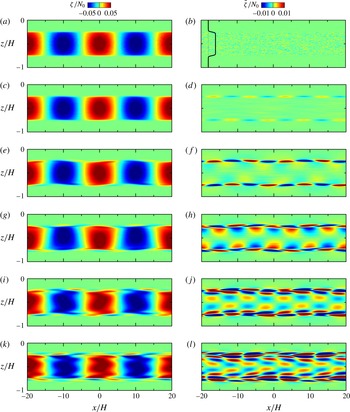
Figure 2 shows snapshots taken from a simulation of a long wave in top-hat-like stratification with no background rotation. The Galerkin analysis finds that the corresponding mode-one disturbance has frequency ${\it\omega}_{0}=0.090N_{0}$ (see figure 1 a). Its associated vorticity together with superimposed noise is shown in figure 2(a). In the corresponding panel to the right the vorticity associated with the parent mode has been subtracted to reveal the initial superimposed background noise.

Figure 2.

Snapshots at six different times of (a,c,e,g,i,k) total vorticity, ${\it\zeta}$ and (b,d,f,h,j,l) corresponding mode-filtered vorticity $\tilde{{\it\zeta}}$ taken from a simulation with a symmetric stratified layer having $D=0.5H$ and $\bar{z}=-0.5H$ , the structure of which is illustrated by the $N^{2}$ profile plotted to the left in the mode-filtered vorticity plot at $Nt=0$ (black curve): (a,b)  $N_{0}t=0$ ; (c,d)  $N_{0}t=6$ ; (e,f)  $N_{0}t=25$ ; (g,h)  $N_{0}t=50$ ; (i,j)  $N_{0}t=100$ ; (k,l)  $N_{0}t=200$ . The initial parent wave amplitude and wavenumber are $A_{0}=0.05H/{\rm\pi}$ and $\ell _{0}=0.1{\rm\pi}/H$ , respectively. The system is not rotating ( $f=0$ ). The time of each snapshot is indicated in the upper-left of each vorticity plot. The colour bars to the upper-right indicate the range for each field. The snapshots are shown in a reference frame moving with the horizontal phase speed of the mode, ${\it\omega}_{0}/\ell _{0}$ . See supplementary movie 1 available at http://dx.doi.org/10.1017/jfm.2016.108.

The snapshots at later times are shown in a frame of reference moving at the horizontal phase speed, ${\it\omega}_{0}/\ell _{0}$ , of the parent mode. The phase of the parent mode changes little between the initial and final times shown. However, its structure is modified significantly by small-scale disturbances. By non-dimensional time $N_{0}t=6$ (approximately one buoyancy period), the growth of superharmonic disturbances (with $\ell =2\ell _{0}$ ) is evident in the mode-filtered vorticity plot to the right. As predicted, the superharmonic disturbances are largest on either flank of the stratified region and the peak is $90^{\circ }$ out of phase with the parent mode. At non-dimensional time $N_{0}t=25$ (approximately four buoyancy periods) these disturbances dominate on the flanks and remain stationary in the frame of reference moving with the horizontal phase speed of the parent mode, consistent with the prediction that the superharmonic disturbance has phase speed $2{\it\omega}_{0}/(2\ell _{0})={\it\omega}_{0}/\ell _{0}$ . At this time the total vorticity field is significantly distorted as a consequence of the superimposed superharmonic disturbances.

As time progresses, due to weakly nonlinear interactions between the disturbance field and the parent mode, the disturbance field becomes non-stationary, slowing with respect to the rightward advance of the parent mode as viewed in the absolute frame of reference. These structures develop finer vertical-scale structures on the flanks while superharmonic disturbances also propagate within the well-stratified region. By non-dimensional time $N_{0}t=200$ (approximately 32 buoyancy periods) the vorticity field of the parent mode is everywhere distorted as a consequence of significant superharmonic disturbances.

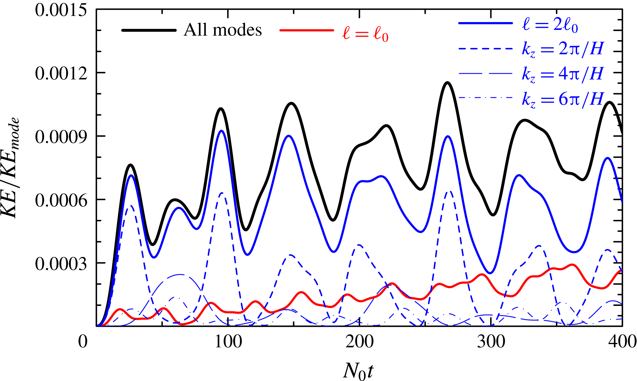
Figure 3 shows the time evolution of the mode-filtered kinetic energy ( ${\it\rho}_{0}(|\tilde{u} |^{2}+|\tilde{w}|^{2})/2$ ) partitioned by horizontal wavenumber. This clearly demonstrates that the energy from the parent mode is transferred primarily to superharmonic disturbances having horizontal wavenumber $\ell =2\ell _{0}$ with a small fraction transferring back to disturbances having the same horizontal wavenumber as the primary mode. The energy in the superharmonics modulates in time as the vertical structure of the superharmonic disturbances change.

Figure 3.

Evolution of the mode-filtered kinetic energy normalized by the initial kinetic energy of the parent mode for the simulation shown in figure 2 but extending up time non-dimensional time $N_{0}t=400$ (about 64 buoyancy periods). Curves show the total disturbance energy (solid) and the fraction associated with disturbances having the same horizontal wavenumber as the parent mode (solid red) and having superharmonic horizontal wavenumber $\ell =2\ell _{0}$ (solid blue). The fraction of the energy in superharmonic disturbances is further partitioned into that associated with sinusoidal waves having vertical wavenumber $2{\rm\pi}/H$ (short-dashed), $4{\rm\pi}/H$ (long-dashed) and $6{\rm\pi}/H$ (dash-dotted).

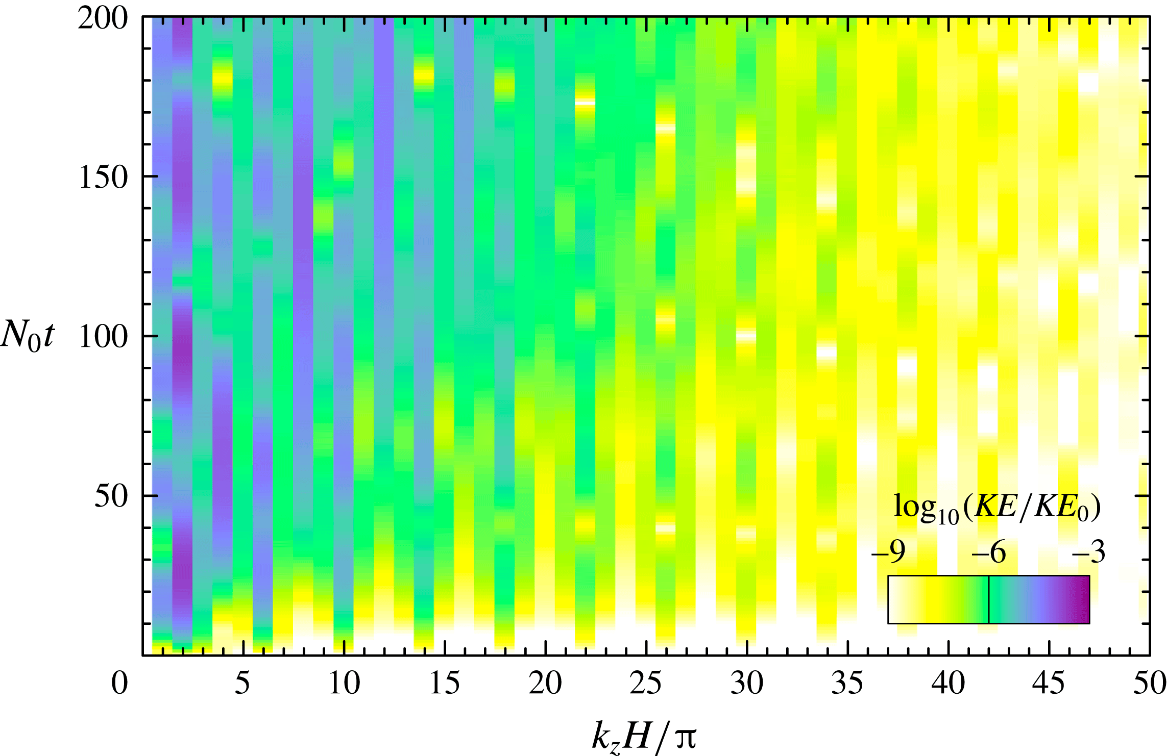
A detailed examination of the vertical wavenumber spectrum as it evolves in time is shown in figure 4. This is computed for disturbances of all horizontal wavenumbers, not just the superharmonics. The time evolution of the leading power spectrum components is shown in figure 3. Because the initial excited disturbances are localized in the vertical the Fourier spectrum exhibits multiple peaks. As time progresses the power peaks sometimes in low even modes, sometimes in low odd modes. But all the time more power is gained by higher vertical wavenumbers.

Figure 4.

Vertical wavenumber spectrum as it evolves in time, shown by the colour scale representing the logarithm of relative disturbance kinetic energy, as indicated to the lower right of the plot. This analysis is performed for the simulation shown in figure 2.

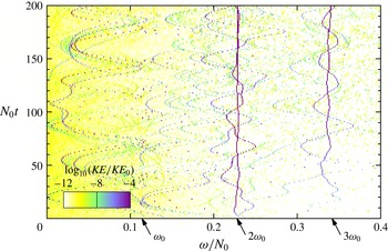
Even at late times this cascade to fine vertical scale is not a consequence of PSI. To demonstrate this, the evolution of the frequency spectrum over time was computed. The frequency itself was determined from the (complex-valued) amplitude $\hat{{\it\zeta}}_{\ell k_{m}}=A_{\ell k_{m}}\exp (\text{i}{\it\phi}_{\ell k_{m}})$ of the mode-filtered vorticity field in horizontal and vertical wavenumber space and from its time derivative $\text{d}\hat{{\it\zeta}}_{\ell k_{m}}/\text{d}t={\dot{A}}_{\ell k_{m}}\exp (\text{i}\dot{{\it\phi}}_{\ell k_{m}})$ . Explicitly, the frequency of the $(\ell ,k_{m})$ mode is

The kinetic energy computed for the $(\ell ,k_{m})$ mode is associated with this frequency. The results are binned so that the sum of kinetic energies associated with disturbances having frequency in the range ${\it\omega}_{i}-{\rm\Delta}{\it\omega}/2<{\it\omega}\leqslant {\it\omega}_{i}+{\rm\Delta}{\it\omega}/2$ is associated with frequency ${\it\omega}_{i}=i{\rm\Delta}{\it\omega}$ for $i=1$ to $1000$ . The bin size is taken to be ${\rm\Delta}{\it\omega}=0.001N_{0}$ .

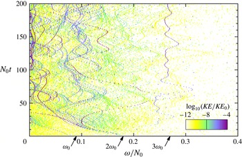
The results of this analysis is shown in figure 5. At early times, the disturbance frequency is sharply peaked moderately below the superharmonic frequency, $2{\it\omega}_{0}$ , with the peak power decreasing in frequency by half over approximately the first two buoyancy periods. For example, at non-dimensional time $N_{0}t=6$ , the peak occurs for frequency ${\it\omega}/N_{0}\simeq 0.1475\pm 0.0010$ with $KE/KE_{0}\simeq 8.7\times 10^{-6}$ . The kinetic energies associated with neighbouring frequencies are two orders of magnitude smaller. At this time a secondary peak occurs moderately below the parent-mode frequency such that $KE/KE_{0}\simeq 6.4\times 10^{-7}$ for ${\it\omega}/N_{0}\simeq 0.0605\pm 0.0010$ .

Figure 5.

As in figure 4 but showing the frequency spectrum as it evolves in time. The arrows along the bottom of the plot indicate the frequencies of the parent mode ( ${\it\omega}_{0}$ ) and its first two superharmonics.

Although the self-interaction of the parent mode results in forcing at frequency $2{\it\omega}_{0}$ and horizontal wavenumber $2\ell _{0}$ , the resulting vertically localized excited disturbance is a superposition of vertical modes. Each of those modes has a frequency determined by $2\ell _{0}$ and the vertical mode number. It is because frequency decreases with increasing vertical mode number (see figure 1 a) that the high vertical modes associated with the vertically localized disturbance have frequency smaller than $2{\it\omega}_{0}$ . As time progresses the kinetic energy becomes distributed over a larger number of peaks that nonetheless are narrow-banded in frequency. Disturbances appear with peak frequencies vacillating about ${\it\omega}_{0}$ while other disturbances have frequencies close to zero and $3{\it\omega}_{0}$ . At no time is there evidence of the spontaneous resonant growth of a subharmonic pair of waves with frequency ${\it\omega}_{0}/2$ .

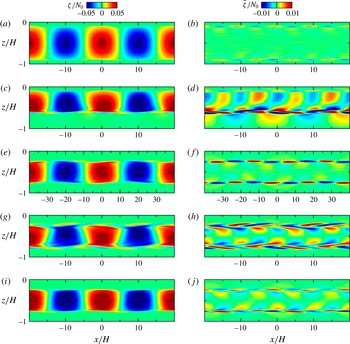
So far analyses have been presented for the ‘base’ simulation with parameters $D=0.5H$ , $\bar{z}=-0.5H$ , $\ell =0.1~{\rm\pi}/H$ , $A_{0}=0.05H/{\rm\pi}$ and $f=0$ . Qualitatively similar results are found from the analyses of simulations run with different parameters. For example, figure 6 shows snapshots at $N_{0}t=50$ taken from simulations in which (a,b) the depth of the strongly stratified region is wider, (c,d) the stratified layer is asymmetrically situated closer to the top of the domain, (e,f) the horizontal wavelength is twice as large, (g,h) the amplitude is twice as large and (i,j) there is background rotation. Each of these pairs of panels should be compared with the two panels in the fourth row of figure 2, corresponding to time $N_{0}t=50$ of the base simulation.

Figure 6.

Snapshots of total vorticity (a,c,e,g,i) and mode-filtered vorticity (b,d,f,h,j) taken at non-dimensional time $N_{0}t=50$ from five different simulations having the same parameters as that shown in figure 2 but with one of the following parameters changed: (a,b) $D=0.8H$ , (c,d) $\bar{z}=-0.35H$ , (e,f) $\ell _{0}=0.05~{\rm\pi}/H$ , (g,h) $A_{0}=0.10H/{\rm\pi}$ and (i,j) $f=0.05N_{0}$ .

In all five cases, superharmonics with $\ell =2\ell _{0}$ develop with disturbance amplitudes being largest on the flanks of the stratified region. The disturbance amplitude is relatively small in the case with $D=0.8H$ . The disturbances are weakly manifest within the stratified region being perturbed by high vertical wavenumber noise, a remnant from the noise used to initialize the simulation. Even after $N_{0}t=400$ , PSI is not observed in this circumstance. In the asymmetric case with $\bar{z}=-0.35H$ (figure 6 c,d), the disturbance amplitude is small on the flank of the stratified region close to the top of the domain, but significant disturbances develop on the lower flank around $z\simeq -0.6H$ . The vorticity field simultaneously exhibits superharmonic disturbances with $\ell =2\ell _{0}$ within the stratified region above the lower interface and it exhibits harmonic disturbances with $\ell =\ell _{0}$ below that interface.

In the simulation with longer parent mode (figure 6 e,f), the disturbance amplitude is relatively large, but the structure of the disturbances on either flank of the stratification is not so complex at this time. However, the simulation with a relatively large-amplitude parent mode (figure 6 g,h) shows significant perturbations at this time with visual evidence for energetic disturbances in modes with $\ell =\ell _{0}$ and $2\ell _{0}$ . In the simulation with background rotation (figure 6 i,j), the time $N_{0}t=50$ corresponds to $ft=2.5$ , or about $0.4$ inertial periods. The disturbance amplitude is relatively smaller at this time, though the structure of the disturbance field is not that different in structure from the simulation with no rotation.

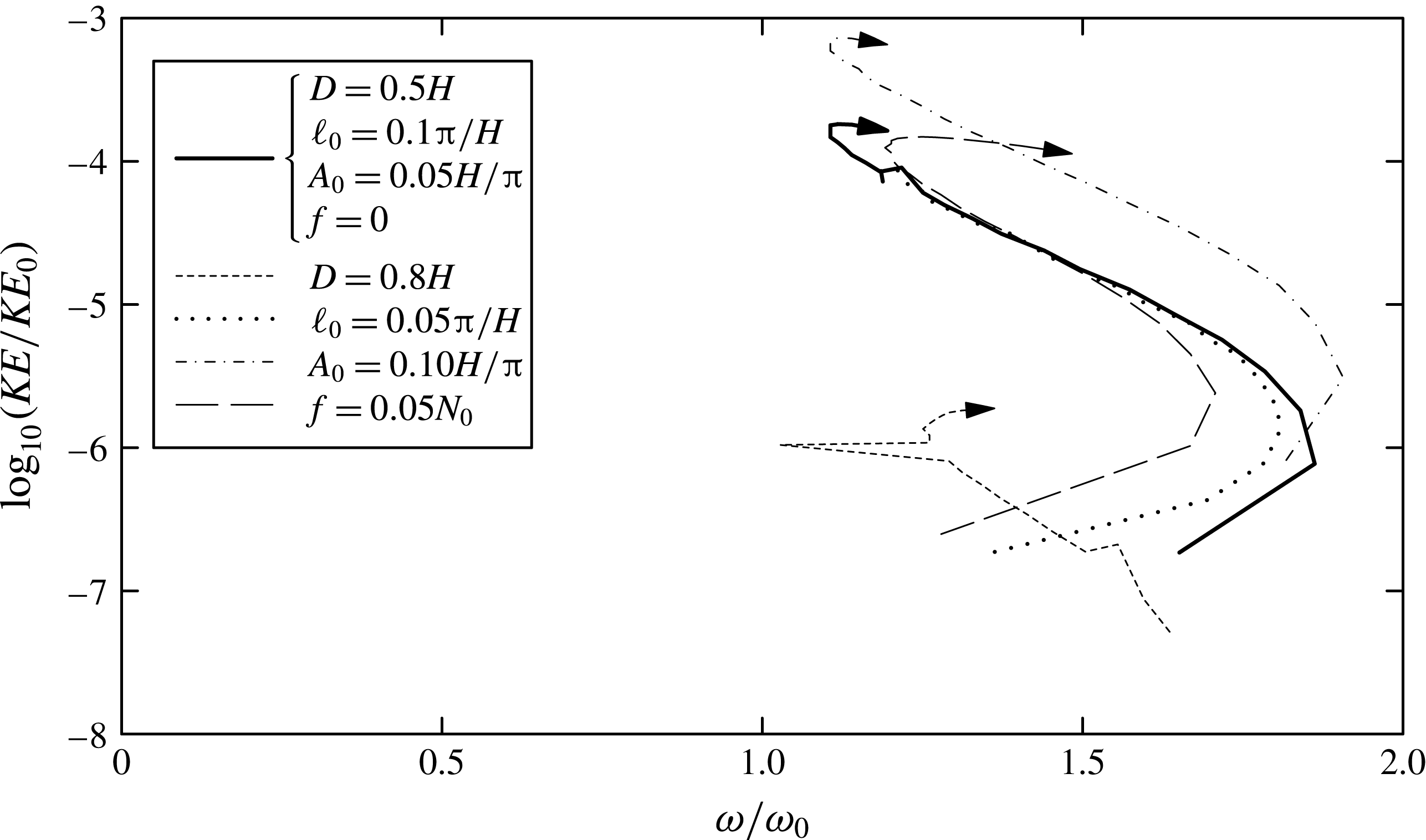
By way of quantitative comparison, we examine the kinetic energy associated with the peak frequency as it evolves over the first few buoyancy periods of the five simulations with vertically symmetric stratification. The results are shown in figure 7. The solid black curve can be identified in this figure from the peak frequencies and corresponding energies shown in figure 5 for times up to $N_{0}t=30$ . In simulations with $\ell _{0}=0.05{\rm\pi}/H$ and with $f=0.05N_{0}$ , the peak frequency follows the same trajectory after the first few time steps, though at times beyond $N_{0}t$ the trajectory of the peak frequency becomes more erratic as lower and higher harmonics gain dominant energy. In the simulation with the larger amplitude parent wave, the peak frequency again becomes manifest with value moderately below $2{\it\omega}_{0}$ , decreasing as the energy grows, and then begins to increase again. Compared with the simulation in which the parent mode has half the amplitude, the kinetic energy of the peak disturbance is four times larger, as expected. In the simulation with $D=0.8H$ , the peak frequency again decreases as the disturbance grows, but the kinetic energy of the peak disturbance is two orders of magnitude smaller than in the corresponding simulation with $D=0.5H$ .

Figure 7.

Value of the relative peak frequency and its corresponding relative kinetic energy computed from five simulations up to five buoyancy periods from the start of the simulation. Arrows indicate the direction of time for each curve. The solid curve is determined from the simulation with snapshots shown in figure 2 with the four parameters indicated in the upper part of the legend. The four other lines are the results from simulations in which one of the four parameters is changed as indicated in the lower part of the legend. In all cases, $\bar{z}=-0.5H$ .

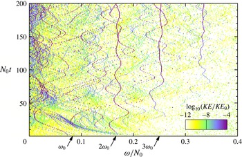
Because the vertical structure of the forcing in the asymmetric case with $\bar{z}=-0.35H$ has non-negligible projection upon the mode-one wave with $\ell =2\ell _{0}$ and because this mode has frequency comparable with the forcing frequency, $2{\it\omega}_{0}$ , the time evolution of the frequency spectrum, shown in figure 8, exhibits strong reinforcement of disturbances with frequency near $2{\it\omega}_{0}$ , as well as of higher harmonics.

Figure 8.

As in figure 5 but showing the temporal evolution of the frequency spectrum computed in a simulation with asymmetric stratification such that $\bar{z}=-0.35H$ . The other simulation parameters are the same as the case shown in figure 2. See supplementary movie 2.

Figure 9.

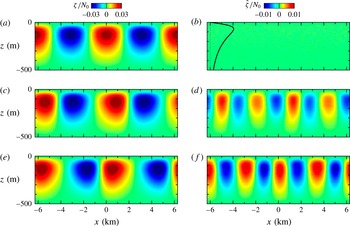
As in figure 2 but for a simulation with stratification representative of the seasonal thermocline: (a,b)  $N_{0}t=0$ ; (c,d)  $N_{0}t=200$ ; (e,f)  $N_{0}t=400$ . The parent mode is initialized with $\ell _{0}=0.001~\text{s}^{-1}$ and amplitude $A_{0}=5~\text{m}$ . The Coriolis parameter is $f=0.01N_{0}$ . See supplementary movie 3.

Returning to the problem of mode-one oceanic internal waves, figure 9 shows snapshots taken from a simulation in which the stratification is representative of the oceanic seasonal thermocline as given by (3.1) with $L_{1}=50~\text{m}$ , $L_{2}=200~\text{m}$ and $z_{0}=-100~\text{m}$ . With these values, the peak squared buoyancy frequency was $\simeq 1.03N_{0}^{2}$ . This simulation was run with background rotation prescribed by $f=0.01N_{0}$ . The simulation was initialized with a small-amplitude long internal mode and the simulation ran up to times $N_{0}t=400$ , corresponding to 64 buoyancy periods or about 0.6 inertial periods. Simulations were run for times an order of magnitude larger and with larger $f$ , but this made little difference to the evolution as far as the growth and evolution of superharmonic disturbances was concerned.

As time progressed, superharmonics were again excited and, superimposed on the parent mode, these acted to enhance and narrow the regions of positive vorticity while the regions of negative vorticity broadened and became weaker. Also evident is the growth of finescale vertical structures dominantly with horizontal wavenumber $2\ell _{0}$ .

The energetics, shown in figure 10, reveal that the majority of energy is transferred initially to superharmonics with frequency $2{\it\omega}_{0}$ and that disturbances with this frequency persist in time while disturbances with frequency $3{\it\omega}_{0}$ also grow to significant amplitude. These disturbances slowly modulate the parent wave, but persist with their structure having largest amplitude around $z=-z_{0}$ . Unlike the simulations in which $N^{2}$ was prescribed with a top-hat-like profile, here $N^{2}$ varies gradually over the depth of the domain, and by comparison the excited disturbances are not as localized in the vertical: their structure maps more closely onto a mode of the system with wavenumber $2\ell _{0}$ . Importantly, the simulations showed no evidence of PSI.

Figure 10.

As in figure 5 but for the simulation with snapshots shown in figure 9, representing the evolution of the frequency spectrum for a mode at a model thermocline.