Nomenclature

UAV

unmanned aerial vehicle

UCAV

unmanned combat aerial vehicle

BaF

Back-and-Forth

tBaF

Multi-Threaded Back-and-Forth

2.0 Literature summary

Zhang et al. calculated the inertia weight and acceleration coefficients in PSO algorithm for the task of UCAV path planning [Reference Zhang, Wu and Wang8]. The chaos theory and the concept of predator-prey were adopted to generate an effective search mechanism by Zhu and Duan and then integrated into the working progress of the Bbiogeoraphy-based optimisation (BBO) when minimising the costs of UCAV paths [Reference Zhu and Duan9]. Duan and Qiao demonstrated how the pigeon-inspired optimisation (PIO) algorithm is applied to plan an air robot [Reference Duan and Qiao10]. Li et al. optimised the flight route of a UCAV system by executing an ABC algorithm assisted with the balance-evolution strategy [Reference Li, Gong and Yang11]. Glowworm swarm optimisation (GSO) algorithm was modified by Tang and Zhou in a manner that the individuals of the GSO are produced with the generation mechanism of the PSO, and PGSO was developed for calculating UCAV paths [Reference Tang and Zhou12]. Zhang and Duan formulated the UAV path planning problem as an optimisation problem with the constraints about the route length, altitude, turning and climbing angles, terrain and non-flight zones and then developed a differential evolution (DE) algorithm-based solver [Reference Zhang and Duan13]. Zhou et al. addressed the bottlenecks of the wolf colony search (WCS) with the help of the complex method, and they introduced CWCS algorithm for planning a UCAV being operated in a fixed altitude environment [Reference Zhou, Zhou and Chen14]. Zhang and Duan simulated the PIO with the predator-prey concept and the results informed the superiority of the PIO with predator-prey concept against the PIO, PSO and DE for the considered three-dimensional battlefield scenario [Reference Zhang and Duan15]. The central force optimisation (CFO) algorithm was modernised by Yangboo Chen et al. in order to path optimisation of a rotary wing vehicle [Reference Chen, Yu, Mei, Wang and Su16]. Zhou et al. specialised the wind-driven optimisation (WDO) by utilising from the quantum rotation gate and quantum non-gate strategies for their path planner [Reference Zhou, Bao, Wang, Qiao and Zhou17]. G.-G. Wang et al. focused on solving UCAV path planning problem with a bat algorithm (BA) and DE hybridisation [Reference Wang, Chu and Mirjalili18].

The GWO algorithm as a UCAV path planner with its standard mathematical model was analysed by Zhang et al., and it was concluded that the GWO is better than its competitors for 17 of 20 test cases [Reference Zhang, Zhou, Li and Pan19]. Liu et al. cleverly determined the space containing the high-potential solutions and investigated how the solution space calibrating approach changes the qualities of the discovered paths by the PSO algorithm [Reference Liu, Zhang, Guan and Delahaye20]. In another study, Liu et al. considered the time variable as the fourth dimension of the UAV path planning problem [Reference Liu, Zhang, Zhang and Guan21]. Luo et al. enhanced the global scanning performance of the BA by modeling the solution update procedures with the quantum rotation and quantum non-gate and a novel BA, quantum encoding BA (QBA), was developed for UCAV path planning problem [Reference Luo, Li and Zhou22]. An extended version of the collective decision optimisation algorithm (CDOA) was announced by Q. Zhang et al. as a trajectory planner [Reference Zhang, Wang, Yang, Ding, Li and Hu23]. Miao et al. boosted the path planning performance of the symbiotic organism search (SOS) with the simplex method and stated that their approach whose name is abbreviated as SMSOS has faster convergence speed than its rivals [Reference Miao, Zhou and Luo24]. Dolicanin et al. analysed the brain storm optimisation (BSO) algorithm over a two-dimensional battlefield [Reference Dolicanin, Fetahovic, Tuba, Capor-Hrosik and Tuba25]. Lin et al. accelerated the convergence speed of the BA after modifying the position update routine. The comparison between the proposed path planner or CPFIBA, BA and another BA hybridisation allowed to prove the robust path planning performance of the CPFIBA [Reference Lin, Tang, Li and Zhao26].

Pan et al. brought together the strong sides of two DE implementations, CIPDE and JADE, and then a versatile path planner was produced [Reference Pan, Liu and Chu27]. Qu et al. switched between the exploration, exploitation, geometric adjustment and optimal adjustment operations of the GWO by serving the reinforcement learning and qualified UAV paths were obtained [Reference Qu, Gai, Zhong and Zhang28]. The proven success of the GWO on the path planning problem also directed Qu et al. for using it when designing another approach called HSGWO-MSOS [Reference Qu, Gai, Zhang and Zhong29]. Yi et al. planned the UCAV paths with the monarch butterfly optimisation (MBO) in which two sub-populations are generated [Reference Yi, Lu and Zhao30]. Yang Chen et al. built a modern neighbourhood learning strategy for the flower pollination algorithm (FPA) and showed that their FPA-based method plans better paths than the A^*, AFP and RRT [Reference Chen, Pi and Xu31]. H. Zhu et al. prepared a well-established comparative study between 12 meta-heuristics for UCAV path planning and concluded that the spider monkey optimisation (SMO) is the most promising one among them [Reference Zhu, Wang, Ma and Li32]. The competitive performance of the standard SMO algorithm gave inspiration to Zhu et al. for developing another method, and they solved the path planning problem with the SMO algorithm using the cooperative coevolution and diversified search direction [Reference Zhu, Wang and Li33].

Zhou et al. fixed the poor local search ability of the BA with the help of the ABC and a new modification of the BA or IBA was described [Reference Xianjin Zhou, Fang and Lan34]. They modeled the enemy threats such as the radars, missiles and anti-aircraft guns and compared the path planning performance of the IBA with the BA, ABC and four more variants of them [Reference Xianjin Zhou, Fang and Lan34]. Xu et al. simulated the mixed-strategy-based gravitational search algorithm (MSGSA) in which adaptive parameter adjustment and Cauchy mutation are utilised for alleviating the premature convergence when calculating UCAV paths [Reference Xu, Jiang and Zhang35]. Jiang et al. combined a special communication mechanism and $\varepsilon $ -level comparison method by aiming at the performance improvement of the GWO and GWOLC was presented. They also integrated a collision avoidance approach referencing the Monte-Carlo tree search into the GWOLC when solving the UAV path planning problem [Reference Jiang, Lyu, Li, Guo and Zhang36]. Another GWO-algorithm-guided path planner was offered by Jarray et al., and experimental studies ensured that the master-slave type parallelisation and cooperative coevolutionary concept dividing the search space give a significant contribution to the path planning performance [Reference Jarray, Al-Dhaifallah, Rezk and Bouallègue37]. Du et al. decided to enhance the local search abilities of the chimp optimisation algorithm (ChOA) by changing the coefficient vector dynamically and foraging strategy for their three-dimensional path planner whose name is IChOA [Reference Du, Zhou, Deng and Luo38].

Wang et al. evaluated the path planning performance of a subtly modified mayfly algorithm (MA) for which exponent decreasing inertia weight strategy, adaptive Cauchy mutation and enhanced crossover operator are consumed [Reference Wang, Pan, Yang, Kong, Snášel and Chu39]. Niu et al. constructed an adaptive neighbourhood for the consumers of the AEO and embedded the quadratic interpolation operator in order to further promoting the searching performance of the NSEAEO [Reference Niu, Yan, Wang and Niu40]. Niu et al. introduced another AEO algorithm-based UCAV path planner known as MAEO [Reference Niu, Yan, Wang and Niu41]. The double-layer coding (DLC), an innovative idea for decreasing the number of superfluous points on the path, was first announced by Jia et al. and then tested with a PSO variant [Reference Jia, Qu and Li42]. Another study published by Jia et al. first focused on designing a point reduction approach for simplifying the intermediate calculations and used it with a GWO-based path planner [Reference Jia, Qu and Li43]. The first implementation of the search and rescue (SAR) optimisation algorithm for solving UAV path planning problem was made by C. Zhang et al. after supporting it with the heuristic crossover strategy [Reference Zhang, Zhou, Qin and Tang44]. Simulated annealing (SA) algorithm was executed as a local search component of the Aquila optimiser (AO) algorithm by Ait-Saadi et al. and a new AO algorithm was experimented on solving UAV path planning problem [Reference Ait-Saadi, Meraihi, Soukane, Ramdane-Cherif and Benmessaoud Gabis45]. Ait-Saadi et al. also served the African vulture optimisation algorithm (AVOA) as a search heuristic of path planning [Reference Ait-Saadi, Meraihi, Soukane, Yahia, Ramdane-Cherif and Gabis46].

Yu et al. cooperated the GWO and DE for their path planner and presented HGWODE algorithm [Reference Yu, Jiang, Wang and Li47]. Chowdhury and De inspired from the GSO algorithm and introduced a new three-dimensional UAV path planner [Reference Chowdhury and De48]. B. Chen et al. first converted the Cartesian coordinate system into spherical space and employed a BA referenced path planner [Reference Chen, Zhang and Yang49]. Huang et al. proposed the ACVDEPSO is a PSO algorithm-backed path planner [Reference Huang, Zhou, Ran, Wang, Chen and Deng50]. X. Zhang et al. utilised from the DE operators for increasing the consumption of information belonging to the qualified solutions in the population of fireworks algorithm (FWA) and generated HDEFWA that demonstrates its efficiency on planning multiple UAVs [Reference Zhang, Zhang and Miao51]. Yu and Luo employed the theory of reinforcement learning for switching the search mechanism and tuning the control parameter values of the cuckoo search (CS) algorithm and a path planner namely RLMSCS was developed [Reference Yu and Luo52]. Honey badger algorithm (HBA) was chosen by Hu et al. and modified with the help of Bernoulli Shift map, piecewise optimal decreasing neighbourhood and horizontal crossing for efficiently searching the optimal UAV paths [Reference Hu, Zhong and Wei53]. An enhanced sparrow search (SSA) algorithm and PSO were executed together by Wang and it was seen that the SSA and PSO hybridisation is a more robust path planner than the SSA and PSO [Reference Wang, Sun, Zhou and Zhu54]. Deng et al. improved the path planning performance of the PSO by integrating the mechanism taken from the GA and dynamic inertia weight adjustment strategy [Reference Deng, Chen, Zhang and Liu55]. A new variant of the immune plasma algorithm (IPA) or hospital IPA (hospIPA) was practised for two- and three-dimensional UAV path planning problem [Reference Aslan56]. A recent study pioneered by Aslan set the Q-learning for altering the pandemic measures in IPA and Q-LIPA was introduced with the purpose of planning UAV paths [Reference Aslan and Demirci57]. Ye et al. augmented the capabilities of the artificial gorilla troops optimiser (GTO) with the combined mutation, quadratic interpolation and random opposition-based learning and tried to plans for a UAV being operated in Meishui Village [Reference Ye, Shao, Zhang and Wang58]. Haris et al. reengineered the calculation procedure of the cognitive and social acceleration coefficients for PSO algorithm and evaluated the capabilities of this PSO implementation on solving UAV path planning problem [Reference Haris, Bhatti and Nam59]. In Table A1 of the Appendix, a summary of the mentioned meta-heuristic-based geometric path planners is given.

3.0 Background of the geometrical path planning problem

The techniques being developed or chosen for solving the UAV or UCAV path planning problem depend on the general model used to describe how a path is obtained. A common model that can also be named as the geometric model is based on selecting points from the previously determined lines and then connecting them by using line segments for obtaining a full path in a battlefield, including enemy threats, each represented with a unique circle of known radius and centre coordinate. Given that a UAV or UCAV will be employed for reaching a target located at point ${p_t} = \left( {{x_t},{y_t}} \right)$ by starting flight from the point ${p_s} = \left( {{x_s},{y_s}} \right)$ and a straight line called the reference line between the ${p_s}$ and ${p_t}$ is drawn. The line drawn between the ${p_s}$ and ${p_t}$ is divided into $D + 1$ equal segments with the help of $D$ points. Each point used to divide the reference line intersects with a line perpendicular to the reference line and the line set $L = \left\{ {{L_1},{L_2}, \ldots ,{L_{D - 1}},{L_D}} \right\}$ is organised [Reference Niu, Yan, Wang and Niu40]. If the set $L$ is guided in a manner that the point ${p_1}$ is chosen from the line ${L_1}$ , the point ${p_2}$ is chosen from the line ${L_2}$ and so on then the selected points are brought together with the ${p_s}$ and ${p_t}$ for generating the point set $P = \left\{ {{p_s},{p_1}, \ldots ,{p_D},{p_t}} \right\}$ , a path generated by each consecutive member of the set $P$ can be described [Reference Aslan7, Reference Niu, Yan, Wang and Niu40].

Even though the linguistic description about how the point set $P$ and corresponding path can be obtained for the geometric model of the path planning problem is straightforward, intense computations and validations guaranteeing that the members of the set $L$ appropriately intersect with the segmentation points and the members of the set $P$ satisfy the line equations are required. To simplify the mentioned calculations and validations, a coordinate system transformation that converts the reference line of the original coordinate system into the horizontal axis of the new coordinate system is applied. When the coordinate system transformation is carried out, the point ${p_k} = \left( {{x_k},{y_k}} \right)$ is ported to the new coordinate system, as in Equation (1) [Reference Aslan7, Reference Niu, Yan, Wang and Niu40]. While the ${\dot x_k}$ is matched with the $\dot x$ -axis value of the transformed point or ${\dot p_k}$ , ${\dot y_k}$ is matched with the $\dot y$ -axis value of the same point. Finally, the angle between the reference line and horizontal axis of the initial coordinate system is represented with the $\theta $ symbol and the result of $arctan)){y_t} - {y_s})/\left( {{x_t} - {x_s}} \right))$ operation is used for its value [Reference Aslan7, Reference Niu, Yan, Wang and Niu40].

(1) \begin{align}\left[ {\begin{array}{*{20}{l}}{{{\dot x}_k}}\\{{{\dot y}_k}}\end{array}} \right] = \left[ {\begin{array}{*{20}{l}}{cos\left( \theta \right)}\quad\quad {}{sin\left( \theta \right)}\\{ - sin\left( \theta \right)}\quad\, {}{cos\left( \theta \right)}\end{array}} \right] \times \left[ {\begin{array}{*{20}{l}}{{x_k} - {x_s}}\\{{y_k} - {y_s}}\end{array}} \right]\end{align}

The $\dot x$ -axis values of the points taken from the set $P$ and ported to the new coordinate system can be calculated immediately by considering the relationship between the reference line, members of the set $L$ and horizontal axis of the coordinate system. Because of the reference line of the original coordinate system is assumed as the $\dot x$ -axis or horizontal axis of the current coordinate system and the members of the set $L$ are vertical lines passing through the segmentation points dividing the reference line equally into $D + 1$ parts, $\dot x$ -axis value of the $ith$ point in the set $P$ becomes equal to the $\dot x$ -axis value of the $ith$ segmentation point and a set containing only $\dot y$ -axis values of the chosen points such as $\left\{ {{{\dot y}_s},{{\dot y}_1}, \ldots ,{{\dot y}_D},{{\dot y}_t}} \right\}$ is enough to identify a UAV or UCAV path. The effect of the transformation on the calculation of the horizontal axis values of the selected points can be visually confirmed with Fig. 1.

Figure 1.

A battlefield with three enemy threats (a), transformed coordinate system (b), hypothetical paths (c) and their mapping to the original coordinate system (d).

The space for which the points ranging from ${p_1}$ to ${p_D}$ are chosen is continuous and relatively small changes on the axis values of a point completely alters the corresponding path in terms of total flight length, effect of the enemy threats and requirement of the turning manoeuvers. In order to numerically measure how the small changes on the axis values of a point alter the total flight length, the effect of the enemy threats and requirement of the turning manoeuvers, a cost or quality calculation schema as in Equation (2) can be served [Reference Aslan7, Reference Niu, Yan, Wang and Niu40]. In Equation (2), $C$ shows the overall path cost, while the ${C_f}$ , ${C_t}$ and ${C_s}$ show the cost of fuel consumption, cost of enemy threats and cost of turning manoeuvers, respectively. Also, the weights of the ${C_f}$ , ${C_t}$ and ${C_s}$ on the $C$ are adjusted by using the ${\lambda _f}$ , ${\lambda _t}$ and ${\lambda _s}$ coefficients whose sum is equal to $1$ [Reference Aslan7, Reference Niu, Yan, Wang and Niu40].

(2) \begin{align}C = {\lambda _f}{C_f} + {\lambda _t}{C_t} + {\lambda _s}{C_s} = {\lambda _f}\mathop \int \nolimits_0^\ell {w_f}d\ell + {\lambda _t}\mathop \int \nolimits_0^\ell {w_t}d\ell + {\lambda _s}\mathop \sum \limits_{j = 1}^D {\emptyset _j}.\end{align}

The calculation of ${C_f}$ needs the integration of the ${w_f}$ term from $0$ to $\ell $ where $\ell $ is the total length of the path. If the ${w_f}$ term is replaced with a positive integer constant such as $1$ , the value of the ${C_f}$ is approximated properly [Reference Aslan7, Reference Niu, Yan, Wang and Niu40]. The integration of the term ${w_t}$ from $0$ to $\ell $ for the ${C_t}$ can also be found by using an appropriate approximation with the acceptable accuracy. Assume that ${p_i}$ and ${p_j}$ are two neighbour points of the set $P$ and ${L_{ij}}$ is the length of line segment between them. Furthermore, it is assumed that the line segment of length ${L_{ij}}$ is divided equally by using ten intermediate points, and the first, third, fifth, seventh and ninth ones are marked. If the line segment of length ${L_{ij}}$ is in the shooting or sensing range of the $kth$ enemy threat, the cost of being detected by the $kth$ enemy threat or ${C_{t,\left( {ij} \right),k}}$ can be calculated with Equation (3) [Reference Aslan7, Reference Niu, Yan, Wang and Niu40]. In Equation (3), the distances between the centre of the $kth$ enemy threat and the first, third, fifth, seventh and ninth intermediate points are represented as $d_{0.1,i,k}^4$ , $d_{0.3,i,k}^4$ , $d_{0.5,i,k}^4$ , $d_{0.7,i,k}^4$ and $d_{0.9,i,k}^4$ and the ${t_k}$ term is used on behalf of the grade or danger level of the $kth$ enemy threat. After checking each line segment in order to decide which enemy threats sense it and summing the cost of being detected, the value of the ${C_t}$ is assigned.

(3) \begin{align}{C_{t,\left( {ij} \right),k}} = \frac{{{L_{ij}}{t_k}}}{5}\left( {\frac{1}{{d_{0.1,i,k}^4}} + \frac{1}{{d_{0.3,i,k}^4}} + \frac{1}{{d_{0.5,i,k}^4}} + \frac{1}{{d_{0.7,i,k}^4}} + \frac{1}{{d_{0.9,i,k}^4}}} \right)\end{align}

For escaping from the enemy threats and reducing the overall flight length, a set of complex turning manoeuvers should be successfully handled by the employed UAV or UCAV system. However, some kinematic constraints of the UAV or UCAV can not allow acceptable turning manoeuvers for each angle. The angle for which a turning manoeuver is carried out can be determined by controlling two vectors generated with the help of three adjacent points. Given that the ${p_j}$ , ${p_{j + 1}}$ and ${p_{j + 2}}$ are three adjacent points of the set $P$ and $\overrightarrow {{p_j}{p_{j + 1}}} $ and $\overrightarrow {{p_{j + 1}}{p_{j + 2}}} $ are two vectors being considered when determining the turning angle as in Equation (4) [Reference Aslan7, Reference Niu, Yan, Wang and Niu40]. If the first three adjacent points are taken into account, ${p_j}$ , ${p_{j + 1}}$ and ${p_{j + 2}}$ are replaced with the ${p_s}$ , ${p_1}$ and ${p_2}$ members of the point set. Similarly, if the last three adjacent points are taken into account, the ${p_{D - 1}}$ , ${p_D}$ and ${p_t}$ are used in the calculations. The decision whether the turning manoeuver is handled or not is made after a comparison between the absolute value of ${\emptyset _j}$ and maximum turning angle also showed as ${\emptyset _{max}}$ symbol. When the absolute value of ${\emptyset _j}$ or $\left| {{\emptyset _j}} \right|$ is found smaller than the ${\emptyset _{max}}$ , it is concluded that the turning manoeuver is in the limitations of the UAV system and an incrementation for the ${C_s}$ is not required. On the contrary, the $\left| {{\emptyset _j}} \right|$ is added to the existing value of the ${C_s}$ for emphasising the failure of the turning. After calculating all of the angles and then comparing them with the ${\emptyset _{max}}$ for understanding which ones violate the limitation, the ${C_s}$ value is determined.

(4) \begin{align}{\emptyset _j} = arctan\left( {\frac{{\parallel \overrightarrow {{p_j}{p_{j + 1}}} \times \overrightarrow {{p_{j + 1}}{p_{j + 2}}} \parallel }}{{\overrightarrow {{p_j}{p_{j + 1}}} \cdot \overrightarrow {{p_{j + 1}}{p_{j + 2}}} }}} \right)\end{align}

4.0 Details of the baf algorithm

The set $\dot L$ containing the transformed line members and the path description method in which points that are located on the lines of set $\dot L$ are connected allow to introduce new planning algorithms. One of these new algorithms is the BaF and it executes a point selection heuristic for generating two main paths and then combines their advantageous parts appropriately in order to find more qualified candidates [Reference Aslan7]. The BaF algorithm first divides each line in the set $\dot L$ equally into $D + 1$ line segments and stores the segmentation points by using point set ${\dot P^1}$ for line ${\dot L_1}$ , point set ${\dot P^2}$ for line ${\dot L_2}$ , and so on. The heuristic of the BaF algorithm decides that the point being selected from the ${\dot P^i}$ where $i$ is equal to or greater than $2$ will be $\dot p_j^i$ by accepting the point $\dot p_j^{i - 1}$ is chosen previously from the set ${\dot P^{i - 1}}$ and $\dot p_j^i$ is not in the effect range of any enemy threat [Reference Aslan7]. When the point $\dot p_j^{i - 1}$ is chosen from the set ${\dot P^{i - 1}}$ , but the point $\dot p_j^i$ of the set ${\dot P^i}$ is in the effect range of an enemy threat, the heuristic tries to select a point from the set ${\dot P^i}$ that is the nearest one to the $\dot p_j^{i - 1}$ after guaranteeing that the point being chosen will be outside the detection ranges of all enemy threats if possible [Reference Aslan7].

The BaF algorithm has an exceptional case about the first line in the set $\dot L$ or ${\dot L_1}$ . Because of there is no line before the ${\dot L_1}$ , the heuristic tries to select a point from the set ${\dot P^1}$ that is the nearest one to the ${\dot p_s}$ and outside the effect ranges of all enemy threats [Reference Aslan7]. The points picked up by the BaF algorithm with the purpose of generating a path from the ${\dot p_s}$ to ${\dot p_t}$ are stored in a set $\dot P = \left\{ {{{\dot p}_1},{{\dot p}_2}, \ldots ,{{\dot p}_D}} \right\}$ for subsequent operations. A formal description for the selection of the first and other points of the path by the BaF is given in Equations (5) and (6), respectively.

(5) \begin{align}{\dot p_1} = \left\{ {\begin{array}{*{20}{l}}{\dot p_j^1,}\quad {}{\mathop {d\left( {t,\dot p_j^1} \right)}\limits_{\forall t \in T} \gt {r_t} \wedge d\left( {{{\dot p}_s},\dot p_j^1} \right) \lt \mathop {d\left( {{{\dot p}_s},\dot p_m^1} \right)}\limits_{\forall \dot p_m^1 \ne \dot p_j^1 \in {{\dot P}^1}} }\\{\dot p_1^1,}\quad\quad\quad\quad\quad\quad\quad {}{otherwise}\end{array}} \right\}\end{align}

(6) \begin{align}{\dot p_i} = \left\{ {\begin{array}{*{20}{l}}\quad\quad\quad{\dot p_j^i,}\quad\quad\quad\quad\quad\quad\quad\quad\quad\quad\quad\quad\,\,\,\, {}{\mathop {d\left( {t,\dot p_j^i} \right)}\limits_{\forall t \in T} \gt {r_t}}\\\quad\quad\quad{\dot p_k^i,}\quad\quad\quad\quad\quad\quad {}{\mathop {d\left( {t,\dot p_k^i} \right)}\limits_{\forall t \in T} \gt {r_t} \wedge d\left( {{{\dot p}_{i - 1}},\dot p_k^i} \right) \lt \mathop {d\left( {{{\dot p}_{i - 1}},\dot p_m^i} \right)}\limits_{\forall \dot p_m^i \ne \dot p_k^i \in {{\dot P}^i} - \left\{ {\dot p_j^i} \right\}} }\\{first{\rm{\;}}of{{\dot P}^i} - \left\{ {\dot p_j^i} \right\},}\quad\quad\quad\quad\quad\quad\quad\quad\,\,\, {}{otherwise}\end{array}} \right\}\end{align}

The line segments near to the point ${\dot p_s}$ can be more advantageous in terms of length and turning manoeuvers for the path of the BaF generated from the start point to the target point. For obtaining another path that is willing to contain advantageous line segments near the point ${\dot p_t}$ , the BaF algorithm can be executed from the ${\dot p_t}$ to ${\dot p_s}$ by guiding the mentioned point selection heuristic. When the BaF algorithm completes the generation of two predecessor or backbone paths, while the first one is calculated from the ${\dot p_s}$ to ${\dot p_t}$ and obtained points are stored in the set $\dot P$ , the second one is calculated from the ${\dot p_t}$ to the ${\dot p_s}$ and obtained points are stored in the set $\ddot P$ , it becomes ready for passing through the subsequent main stage generating new candidates by combining the appropriate parts of the predecessor paths. For deciding which parts of the predecessor paths are combined, the BaF algorithm assigns a similarity score to each matched line segment of the paths as detailed in Equation (7) [Reference Aslan7]. In Equation (7), ${s_j}$ is used on behalf of the similarity score calculated for the $jth$ line segments of the paths derived from the sets $\dot P$ and $\ddot P$ . Also, while the ${\dot p_j}$ and ${\dot p_{j + 1}}$ show the $j$ and $j + 1$ indexed points in the set $\dot P$ , the ${\ddot p_j}$ and ${\ddot p_{j + 1}}$ show the $j$ and $j + 1$ indexed points in the set $\ddot P$ . If the difference between the $jth$ and $\left( {j + 1} \right)th$ points of the $\dot P$ and $\ddot P$ decreases, the similarity score increases, and the change trend between the segments of the paths is identified more subtly.

(7) \begin{align}{s_j} = 1/\left( {\left| {{{\dot p}_j} - {{\ddot p}_j}\left| + \right|{{\dot p}_{j + 1}} - {{\ddot p}_{j + 1}}} \right|} \right)\end{align}

Assume that the similarity score calculated for the $jth$ segments of the paths is higher than the similarity scores calculated for the other line segments. In order to generate the first candidate path whose points are stored in the set ${\dot C^1}$ , the points indexed from $1$ to $j - 1$ of the set $\dot P$ are chosen directly and the elements of the set ${\dot C^1}$ indexed from $1$ to $j - 1$ are fixed to these chosen points [Reference Aslan7]. Moreover, the $\dot c_j^1$ and $\dot c_{j + 1}^1$ elements of the set ${\dot C^1}$ are determined as the ${\dot p_j}$ and ${\dot p_{j + 1}}$ , if the path represented with the set $\dot P$ is better than the path represented with the set $\ddot P$ . If the path derived from the set $\ddot P$ is better than the path derived from the set $\dot P$ , the $\dot c_j^1$ and $\dot c_{j + 1}^1$ elements of the set ${\dot C^1}$ are fixed to the ${\ddot p_j}$ and ${\ddot p_{j + 1}}$ [Reference Aslan7]. The remaining elements of the set ${\dot C^1}$ are temporarily matched with the corresponding elements of the $\dot P$ and calculated again by using Equation (8) [Reference Aslan7]. In Equation (8), ${\dot p_i}$ and ${\ddot p_i}$ are the $ith$ elements of the sets $\dot P$ and $\ddot P$ and the value of the index $i$ ranges from $j + 2$ to $D$ as guessed. If the newly calculated $ith$ element for the set ${\dot C^1}$ improves the overall path quality, the initial value of the $ith$ element is updated. Otherwise, the $\dot c_i^1$ preserves its initially inherited assignment [Reference Aslan7].

(8) \begin{align}\dot c_i^1 = \left( {{{\dot p}_i} + {{\ddot p}_i}} \right)/2.\end{align}

The second candidate path whose points are stored in the set ${\dot C^2}$ is tried to be generated by focusing on the protection of the points indexed from $j + 2$ to $D$ belonging to the set $\dot P$ . Because of this reason, the initial assignments for the set ${\dot C^2}$ are carried out as the initial assignments for the set ${\dot C^1}$ and then the points indexed from $1$ to $j - 1$ belonging to the set ${\dot C^2}$ are calculated again by guiding Equation (8). If the quality of the path corresponding to the set ${\dot C^2}$ increases with the calculated point, a replacement between the old and new elements is conducted.

The third and fourth candidate paths of the BaF algorithm are generated by referencing the idea based on protecting the advantageous points and line segments of the path related with the set $\ddot P$ . When generating the third candidate path whose points are stored in the set ${\dot C^3}$ , the points indexed from $1$ to $j - 1$ of the set $\ddot P$ are chosen directly and the elements of the set ${\dot C^3}$ indexed from $1$ to $j - 1$ are fixed to these chosen points. Also, the $\dot c_j^3$ and $\dot c_{j + 1}^3$ elements of the set ${\dot C^3}$ are inherited from the matched members of the set $\dot P$ , if the path drawn by using the set $\dot P$ is better than the path drawn by using the set $\ddot P$ . Otherwise, the ${\ddot p_j}$ and ${\ddot p_{j + 1}}$ are used for setting the initial values of the $\dot c_j^3$ and $\dot c_{j + 1}^3$ elements, respectively. The remaining elements of the set ${\dot C^3}$ are temporarily filled with the corresponding elements of the $\ddot P$ and calculated again one by one after executing Equation (8). If the point found by executing Equation (8) increases the path quality, a replacement procedure for the current and calculated points is applied.

The fourth candidate path for which the set ${\dot C^4}$ is used in order to store the selected points is tried to be generated by focusing on the protection of the elements indexed from $j + 2$ to $D$ belonging to the set $\ddot P$ . Due to this main reason, the initial assignments for the set ${\dot C^4}$ are conducted as in the initial assignments for the set ${\dot C^3}$ and then the points indexed from $1$ to $j - 1$ of the set ${\dot C^4}$ are determined again by guiding Equation (8). If the quality of the path corresponding to the set ${\dot C^4}$ increases with the determined point, a replacement with the old and new elements is done. When the generation of the candidate paths is completed, the BaF algorithm makes a comparison among the candidates and their predecessors and chooses the best one as its result.

5.0 Details of the multi-threaded baf algorithm

The BaF algorithm controls the points that divide each line of the set $\dot L$ into $D + 1$ segments equally, and its heuristic selects a point from each line for representing a backbone path. Moreover, the BaF algorithm can benefit from the computational power of a multi-core or multi-threaded system in a manner that a core or thread controls the points dividing a predetermined part of each line of the set $\dot L$ into $D + 1$ line segments equally. Assume that there are $M$ different threads and the lower and upper bounds of the lines ranging from ${\dot L_1}$ to ${\dot L_D}$ are showed as $LB$ and $UB$ , respectively. For determining the lower and upper bounds of the predetermined part of a line in the set $\dot L$ that will be processed later by the $mth$ thread, Equations (9) and (10) can be employed.

(9) \begin{align}L{B_m} = LB\end{align}

(10) \begin{align}U{B_m} = LB + m \times \frac{{\left( {UB - LB} \right)}}{M}\end{align}

As easily seen from Equations (9) and (10), while the lower bound is the same for each thread, their upper bounds are incremented gradually until reaching the upper bound. By setting the lower bounds of the threads to the $LB$ value and incrementing their upper bounds gradually, each thread except the first one can get a chance of finding a qualified path if it exists within the search space of the previous thread or threads. Moreover, determining the lower and upper bounds for the threads individually allows them to carry out a more sensitive search by keeping the computational complexity per thread as same with the computational complexity of the single-threaded BaF algorithm. In Fig. 2, how four threads adjust the lower and upper bounds and how the first backbone path from ${\dot p_s}$ to ${\dot p_t}$ is generated by each one are illustrated over a battlefield for which the number of segmentation points or $D$ is set to $5$ .

Figure 2.

Determination of the backbone paths from ${\dot p_s}$ to ${\dot p_t}$ by the first (a), second (b), third (c) and fourth (d) threads.

When the bounds for the $mth$ thread is determined, it divides the related part of each line of the set $\dot L$ equally into $D + 1$ small line segments with the help of $D$ points and then selects the points by guiding the heuristic and applies the mentioned combination method of the BaF for generating a UAV or UCAV path. Because the lower and upper bounds of the last thread are matched with the initial lower and upper bounds of a line, the path found by this thread becomes equal to the path of the standard and single-threaded implementation of the BaF algorithm and it is guaranteed that the multi-thread-based specialisation of the BaF generates a final path whose quality is better than or at least equal to the quality of the path discovered by the single-threaded BaF. The step-by-step description about how the $mth$ thread of the multi-threaded BaF algorithm selects the point from the first line and how the $mth$ thread of the multi-threaded BaF algorithm selects the points from the second and other lines are given in Algorithms 1 and 2.

Algorithm 1. Selection procedure from the first line for the $mth$ thread

Algorithm 2.

Selection procedure from the remaining lines for the $mth$ thread

The thread-based specialisation on the lower and upper bounds can also bring some advantageous sides about the local and global search mechanics together. While the threads with the small indexes determine the upper bounds relatively close to the common lower bound and apply the selection heuristic for choosing points on the short parts of the lines in the set $\dot L$ , the threads with the higher indexes determine the upper bounds far away from the common lower bound. As an expected result of the increased distance between the lower and upper bounds, the threads with the higher indexes reflect more global search characteristics compared to the other threads. If a path is calculated for a UAV or UCAV being operated in a battlefield including enemy threats distributed widely open, the initial threads of the thread pool are likely to discover more short and safe candidates because of their subtly narrowed search spaces. On the other hand, if a path is calculated for a UAV or UCAV being operated in a battlefield including enemy threats located closely each other, some threads can be capable of finding more qualified solutions by considering their extended bounds. The BaF algorithm managing a set of threads as described above with the purpose of calculating paths is called the multi-threaded BaF algorithm, and tBaF abbreviation will be used for the remaining parts of the study.

The computational complexity or running time of the BaF and tBaF can change whether the selection of a point in the set ${\dot P^2}$ or other subsequent sets requires the control of $D - 1$ remaining points or not. Assume that each selection from the set ${\dot P^2}$ or other subsequent ones requires the control of $D - 1$ remaining points. Also, it is assumed that the decision about the point being controlled is in the effect range of an enemy threat or not is made after checking all of $N$ enemy threats and the cost of each check is a constant in Big- $O$ notation and showed as $O\left( 1 \right)$ . Moreover, the cost of other operations for a point can be represented by using a constant with computational complexity of $O\left( 1 \right)$ and the total cost can be found by summing $O\left( N \right)$ and $O\left( 1 \right)$ . If the total cost stemmed from the control operations of enemy threats or $O\left( N \right)$ is accepted as sufficiently greater than the cost of other operations for a point or $O\left( 1 \right)$ , the summation of $O\left( 1 \right)$ and $O\left( N \right)$ can be taken equal to $O\left( N \right)$ by utilising from the properties of the asymptotic notation. Because of there are $D - 1$ points being controlled, a multiplication between $D - 1$ and $O\left( N \right)$ and its result found as $O))D - 1) \times N)$ can be used to emphasise the cost of selecting a point from one of the lines ranging from ${\dot L_2}$ to ${\dot L_D}$ . However, it should be considered that before executing the for loop in lines $21$ - $42$ of Alg. (2), an extra control about the preselected point is carried out with the cost of $O\left( N \right)$ and the cost of selecting a point from one of lines ranging from ${\dot L_2}$ to ${\dot L_D}$ becomes equal to $O\left( {D \times N} \right)$ .

The selection heuristic referenced by the BaF and tBaF differentiates the first line or ${\dot L_1}$ in the set $\dot L$ from the other lines of the same set. When selecting a point in the set ${\dot P^1}$ of line ${\dot L_1}$ , a preselected point does not exist and all of $D$ points are evaluated. Given that the decision about the considered point is in the effect range of an enemy threat or not is made after checking all of $N$ enemy threats and the total cost originated from the controls about enemy threats and other operations for a point is $O\left( N \right)$ . Because of there are $D$ points in the set ${\dot P^1}$ , the cost of selecting a point from the line ${\dot L^1}$ is found as $O\left( {D \times N} \right)$ . By considering that each line in the set $\dot L$ of size $D$ is related with a computational complexity of $O\left( {D \times N} \right)$ , the effect of the heuristic on the the running time of the BaF and tBaF is calculated as $O\left( {D \times D \times N} \right)$ or $O\left( {{D^2} \times N} \right)$ for the worst-case scenario.

As stated previously, the selection of a point in the set ${\dot P^i}$ of line ${\dot L^i}$ where $i$ is greater than $1$ can be concluded immediately after checking the point $\dot p_j^i$ , if the point $\dot p_j^{i - 1}$ in the set ${\dot P^{i - 1}}$ of line ${\dot L^{i - 1}}$ is selected. When the point $\dot p_j^i$ is not in the effect range of any enemy threat, it is chosen without controlling other $D - 1$ points. Assume that each selection from the set ${\dot P^2}$ or other subsequent sets is concluded immediately after validating that the preselected point is outside the effect range of all $N$ enemy threats by executing the for loop in lines $11$ - $16$ of Alg. (2) with the computational complexity of $O\left( N \right)$ . Also, by considering that there are $D - 1$ lines from ${\dot L^2}$ to ${\dot L^D}$ , the total cost of selecting $D - 1$ points from the sets related with these lines is found equal to $O))D - 1) \times N)$ . Finally, the burden of the heuristic on the running time of the BaF and tBaF is calculated as the sum of the cost of $O\left( N \right)$ stemmed from the calculations for the first line and the cost of $O))D - 1) \times N)$ stemmed from the calculations for the subsequent lines and showed as $O\left( {D \times N} \right)$ when the best-case scenario guarantees the safety of the whole path except the segment between the ${\dot p_s}$ and $\dot p_j^1$ is taken into account.

Both BaF and each thread of tBaF invoke an objective function formulated as in Equation (2) for assigning the qualities of the predecessor paths and candidates derived from them. For determining the qualities of two predecessor paths and initial qualities of four candidate paths represented with the sets ${\dot C^1}$ , ${\dot C^2}$ , ${\dot C^3}$ and ${\dot C^4}$ , the BaF and tBaF algorithms call the objective function ${\rm{six}}$ times. Until finalising the point members of the ${\dot C^1}$ and ${\dot C^2}$ , the objective function is called $D - 2$ times in total. Similarly, until finalising the point members of the ${\dot C^3}$ and ${\dot C^4}$ , the objective function is called $D - 2$ times and total number of calls reaches to $2D + 2$ . If the total number of calls or $2D + 2$ is multiplied with the computational complexity of the objective function that is equal to $O\left( {D \times N} \right)$ , the load of the function invocations on the overall running time is found as $O\left( {{D^2} \times N} \right)$ . By considering the polynomial domination of the $O\left( {{D^2} \times N} \right)$ compared to the computational costs of the best- and worst-case selection scenarios, the running time of the BaF or tBaF for a thread can be showed with the $O\left( {{D^2} \times N} \right)$ .

6.0 Experimental studies

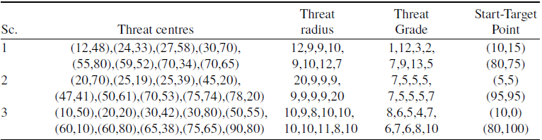
The qualities of the paths being calculated by the tBaF algorithm can change according to the start and target points, enemy threats, centre coordinates and detection ranges of them and the number of segmentation points. For these reasons, three different hypothetical battlefield scenarios whose details about the number of enemy threats, their centre coordinates, sensing ranges and grades showing the danger levels are summarised in Table A2 of the Appendix were chosen [Reference Niu, Yan, Wang and Niu40]. Furthermore, for evaluating how the number of threads affects the path planning performance of the tBaF algorithm, 12 different constants including $2$ , $4$ , $6$ , $8$ , $12$ , $16$ , $20$ , $24$ , $32$ , $48$ , $56$ and $64$ were used. 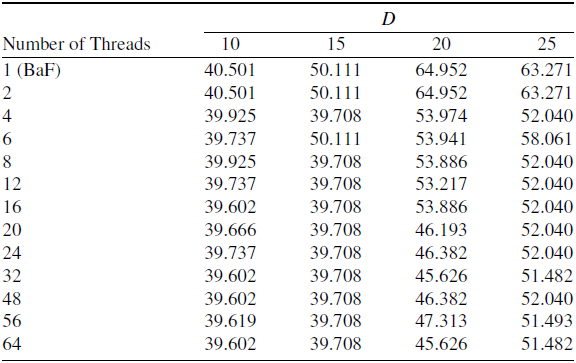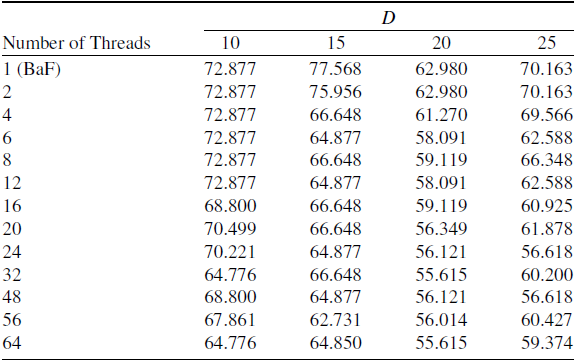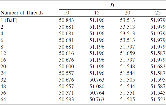Each test case generated by setting the number of segmentation points or $D$ to $10$ , $15$ , $20$ and $25$ was solved with the tBaF algorithm and the qualities of the discovered paths estimated over Equation (2) were presented in Table 1 for the Scenario- $1$ , Table 2 for the Scenario- $2$ and Table 3 for the Scenario- $3$ .

Table 1.

Results of the tBaF with different number of threads for Scenario- $1$

Table 2.

Results of the tBaF with different number of threads for Scenario- $2$

Table 3.

Results of the tBaF with different number of threads for Scenario- $3$

The results given in Tables 1, 2 and 3 allow to validate a general and expected assumption about that the qualities of the paths being planned by the tBaF can be improved when the higher number of threads is chosen. As stated earlier, each thread in the tBaF algorithm uses the same lower bound, while the upper bounds are increased gradually until the upper bound of the last thread becomes equal to the previously determined upper bound of the line. Due to the idea lying behind the subtly determination of the lower and upper bounds for each thread, the probability of finding qualified paths by the tBaF is increased intrinsically with the higher number of threads. When the configuration of the tBaF algorithm for which a better path is obtained is considered, it is easily seen that the number of threads should be chosen equal to or greater than $16$ for Scenario- $1$ and Scenario- $2$ and $20$ for Scenario- $3$ . If a more detailed investigation is carried out on the basis of the appropriate value being assigned to the number of threads, the tBaF algorithm should be started with $32$ or $64$ threads for 10- and $20$ -dimensional cases of Scenario- $1$ , $56$ threads for $15$ -dimensional case of Scenario- $1$ , $24$ or $48$ threads for $25$ -dimensional case of Scenario- $1$ . Also, the tBaF algorithm should be started with $32$ or $64$ threads for 10- and $20$ -dimensional cases of Scenario- $2$ , $56$ threads for $15$ -dimensional case of Scenario- $2$ , $24$ or $48$ threads for $25$ -dimensional case of Scenario- $2$ . Finally, the tBaF algorithm performs better by setting the number of threads to $24$ or $48$ for $10$ -dimensional case of Scenario- $3$ , $32$ or $64$ for 15- and $20$ -dimensional cases of Scenario- $3$ , $64$ for $25$ -dimensional case of Scenario- $3$ . In order to make a visual comparison between the paths found by the tBaF with $32$ threads and BaF, Figs 3, 4 and 5 can be investigated.

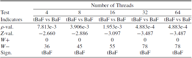
The decision about whether the thread-based parallelisation and subtly designed search bound adjustment strategy give an undeniable contribution or not can be made by comparing the results of the tBaF and BaF algorithms over a statistical test. The Wilcoxon signed-rank test is served commonly when determining which competitor shows a statistically better performance. If the significance level or $\rho $ indicator yielded via the test is less than a constant usually set to $0.05$ , the hypothesis stating that the new method outperforms the previous method is accepted as true [Reference Aslan and Erkin60]. The values of the indicators obtained by the Wilcoxon signed-rank test-based comparison between the tBaF configured with $4$ , $8$ , $16$ , $32$ and $64$ threads and BaF were given in Table 4. In Table 4, the $Z$ value is matched with the standardised test statistics. Also, while the sum of ranks for which the tBaF finds more qualified paths than the BaF corresponds to the $W - $ , the sum of ranks for which the BaF finds more qualified paths than the tBaF corresponds to the $W + $ in the same table. When the $\rho $ values belonging to the comparison between the tBaF and BaF algorithms are investigated, it is understood that the superiority of the tBaF against the BaF is statistically apparent. Although the formula used to assign the cost to the discovered paths limits the numerical differences among the solutions, the tBaF algorithm is capable of calculating more safe, fuel efficient and manoeuverable paths than the BaF for almost all 12 cases, and qualities of the paths are enough to generate statistical significance in favour of it.

Table 4.

Statistical comparison between the tBaF and BaF algorithms

Figure 3.

The paths of the tBaF and BaF for $10$ (a), $15$ (b), $20$ (c) and $25$ -dimensional (d) cases of the Scenario- $1$ .

Figure 4.

The paths of the tBaF and BaF for $10$ (a), $15$ (b), $20$ (c) and $25$ -dimensional (d) cases of the Scenario- $2$ .

Figure 5.

The paths of the tBaF and BaF for $10$ (a), $15$ (b), $20$ (c) and $25$ -dimensional (d) cases of the Scenario- $3$ .

In order to understand the status of the tBaF among other techniques, a set of comparisons between its configuration with $32$ threads, BaF and strong meta-heuristic or heuristic geometric path planners including ABC, GA, GAPSO, MFO, SSA, PFA, SBO, SCA, ECTLBO, HSGWO-MSOS, CIPSO, GWO, AEO and NSEAEO was carried out. For experimenting, the path planners except the tBaF and BaF algorithms, the population size, colony size or number of food sources was set to $30,$ and the maximum evaluation number was taken equal to $6000$ [Reference Niu, Yan, Wang and Niu40]. Also, they were tested $30$ times for each case of the battlefield scenarios, and the best path found and the corresponding path quality were recorded at the end of a run. The qualities of the recorded paths were used to determine the best, worst, mean best quality scores in addition to the standard deviations and summarised over Table A3 of Appendix for Scenario- $1$ , Table A4 of Appendix for Scenario- $2$ and Table A5 of Appendix for Scenario- $3$ with the results of the tBaF and BaF algorithms. Because the tBaF and BaF algorithms are deterministic, their standard deviations are reported as zero, and the ranks of the algorithms rather than the tBaF and BaF are found by considering the mean best quality values. The average and overall ranks reported in Tables A3, A4 and A5 provide strong evidences about the competitive and promising performance of the tBaF algorithm against not only the BaF, but also the other well-known meta-heuristic-based path planners. While the tBaF algorithm is ranked as the second-best path planner and lags behind only the NSEAEO for the Scenario- $1$ , it is ranked as the third-best path planner and lags behind the AEO and NSEAEO for the Scenario- $2$ . Moreover, for the Scenario- $3$ , the tBaF is ranked as the best path planner on the basis of the average ranks and proves its promising performance by being listed in the top three path planners among all 16 techniques. In Fig. 6, stacked bar charts related to the top seven competitors were plotted for a quick comparison.

Figure 6.

Bar charts visualising the status of the top seven competitors for the Scenario- $1$ (a), Scenario- $2$ (b) and Scenario- $3$ (c).

In the tBaF algorithm, a thread calculating a path by guiding the rules of the BaF algorithm and subtly determined lower and upper bounds for the lines of the set $\dot L$ makes $2D + 2$ calls to the function assigning the quality of the path. When the tBaF algorithm is employed with the purpose of finding a path for 10- and $15$ -dimensional cases of a battlefield scenario, a thread of the tBaF makes $22$ and $32$ calls to the function determining the quality of a path. Similarly, when the tBaF algorithm is executed for 20- and $25$ -dimensional cases of a battlefield scenario, $42$ and $52$ calls to the function determining the quality of a path are carried out. Even though the tBaF with $32$ threads requires nearly $272$ times less function calls per thread and $8.5$ times less function calls in total for $10$ -dimensional cases, $187$ times less function calls per thread and $6$ times less function calls in total for $15$ -dimensional cases, $142$ times less function calls per thread and $5$ times less function calls in total for $20$ -dimensional cases, $115$ times less function calls per thread and $4$ times less function calls in total for $25$ -dimensional cases compared to the other tested meta-heuristics, the carefully designed point selection procedure inherited by the BaF and specially determined searching bounds for each thread together allow the tBaF to outperform most of its rivals and being listed in the top three path planners among them. The concept introduced by the tBaF algorithm about the usage of multiple threads brings intrinsic advantages for the sensitivity of the search. While the threads with the higher indexes try to select points distributed on the larger line parts whose lengths are proportional to the values of the thread indexes and positively contribute to the global search capability of the tBaF, the threads with the lower indexes execute the selection heuristic for more specialised and smaller line parts. Because more specialised and smaller line parts are evaluated, the local search characteristics become dominant and balance the effects of the other threads.

The computational complexity of the operations executed by a thread in the tBaF algorithm is equal to the computational complexity of the BaF algorithm. As an expected result of this situation, it is assumed that the execution times of the tBaF and BaF algorithms are measured roughly same, if the number of threads for the tBaF algorithm is chosen appropriately according to the capabilities of the running environment. 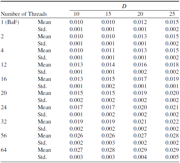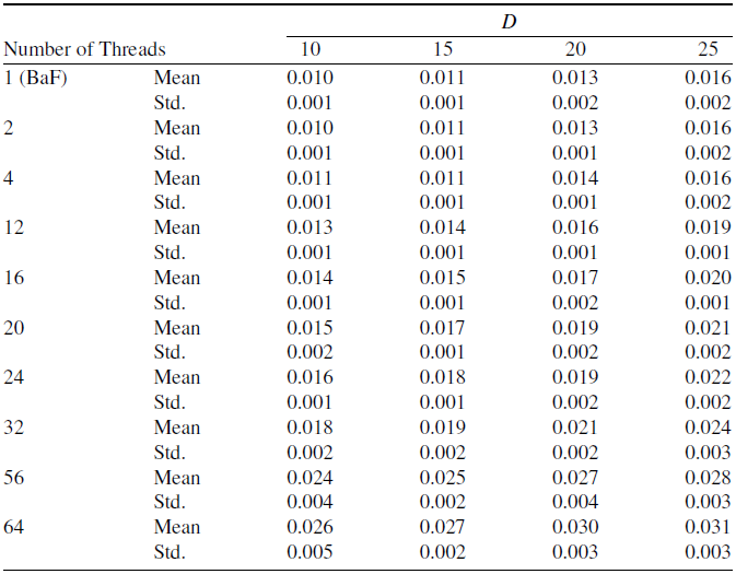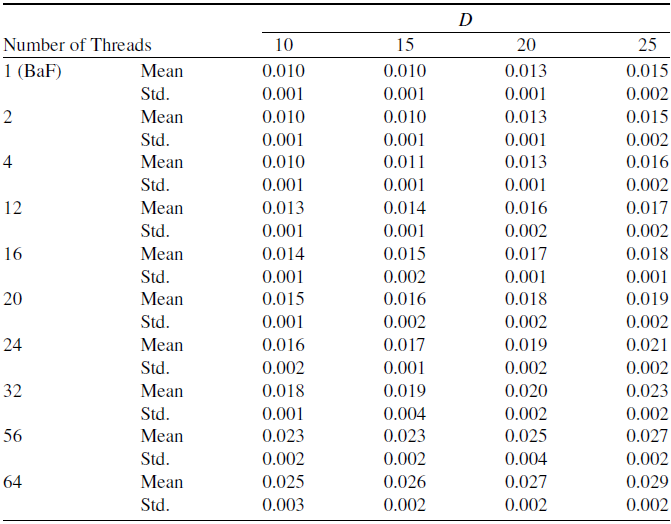In order to decide whether the assumption about the execution times is correct or not, both the tBaF and BaF algorithms coded in C programming language were tested $30$ times for each case of the battlefield scenarios by using a computer containing a dual Intel Xeon E5-2682 v4 processor. For creating and managing the threads of the tBaF algorithm, the pthreads library was used. The elapsed times in terms of seconds required to complete a run were recorded for the tBaF and BaF algorithms. The average elapsed times and related standard deviations were determined by using the recorded values and then presented in Tables 5, 6 and 7. The results presented in Tables 5, 6 and 7 provide enough evidences about the correctness of the initial assumption related to the execution times of the tBaF and BaF algorithms. If the number of threads for the tBaF algorithm is chosen equal to or less than $32$ , the burden stemming from the thread fork and join operations on the execution time of the tBaF can be acceptable or even negligible by considering the execution time of the BaF. Because the processor in the running environment has $16$ physical cores with $32$ threads, the thread configuration of the tBaF exceeding the limitations of the single processor requires more time in order to manage the fork and join operations and brings a considerable amount of load to the execution time of the algorithm. While the difference between the average execution times of the tBaF with $32$ threads and BaF is $0.008$ seconds at most for $25$ -dimensional test cases, the difference between the average execution times of the tBaF with $64$ threads and BaF becomes equal to $0.015$ seconds at most and informs about how the organisation of the addition $32$ threads changes the time spent until the completion.

Table 5.

Elapsed times of the tBaF with different numbers of threads for Scenario- $1$

Table 6.

Elapsed times of the tBaF with different number of threads for Scenario- $2$

Table 7.

Elapsed times of the tBaF with different number of threads for Scenario- $3$