1 Introduction
The hydrodynamic stability of mixed convection in vertical ducts filled with a porous medium is of fundamental importance in practical applications. Due to the presence of inter-connected voids, a porous medium has a large surface area to volume fraction and is a good candidate for heat transfer enhancement applications. One of the major heat transfer applications is in the electronic industry. Starting with micro-scale electronic equipment (due to the miniaturization of integrated circuits and the assemblage in small volumes (Kamath, Balaji & Venkateshan Reference Kamath, Balaji and Venkateshan2011)) to macro-scale electrical transformer (Tang, Wu & Richardson Reference Tang, Wu and Richardson2002) or giant uninterruptible power supply (UPS), design of good heat transfer equipment has become a challenge to the industry. Use of porous media such as metal foams has attracted the attention of many researchers due to their desirable flow and thermal characteristics (Calmidi & Mahajan Reference Calmidi and Mahajan2000). An open cell metal foam consists of a solid matrix containing a large volume fraction of interconnected voids or pores and is used for heat exchangers (Kurtbas & Celik Reference Kurtbas and Celik2009; Dukhan Reference Dukhan2013; Zhang, Li & Nakayamayao Reference Zhang, Li and Nakayamayao2015), electronics cooling (Rachedi & Chikh Reference Rachedi and Chikh2001; Bhattacharya & Mahajan Reference Bhattacharya and Mahajan2002), energy absorption (Lefebvre, Banhart & Dunand Reference Lefebvre, Banhart and Dunand2008), etc. For example, to exchange the heat of a macro-scale electronic device from the system to the surroundings, a vertical rectangular duct whose height and depth are extremely large compared to its width, filled with a fluid-saturated open cell metal foam, can be considered inside the system. The heat generated from the system can be treated as a constant heat flux or linearly varying temperature on both surfaces across the width of the duct. A steady parallel flow due to an external pressure gradient can be considered through it to exchange the heat from the system to the surroundings. For faster cooling one may enhance the velocity of the steady flow, or increase the gap between two channel (in the case of a rectangular duct) walls. In this situation, the steady flow may not remain stable and the exchange of heat from the system to the surroundings may be affected due to the mixing of different fluid layers. Therefore, before installing this type of heat exchanger in the system it is essential to understand the fluid flow and heat transfer mechanism through a channel filled with an open cell metal foam or a highly permeable porous medium, especially in the transition state.
The above flow is caused by the action of the buoyancy force and an external pressure gradient. The stability analysis of this flow has directed intense research efforts toward its understanding, and the extensive work on this topic is well reviewed in the book by Nield & Bejan (Reference Nield and Bejan2013). Most of the works on this topic, starting from the pioneering work of Gill (Reference Gill1969) in natural convection to recent works in mixed convection (Barletta Reference Barletta2016; Bera & Khandelwal Reference Bera and Khandelwal2016), are limited to linear stability analysis only. To the best of our knowledge, although some attempts (Qin & Kaloni Reference Qin and Kaloni1993; Scott & Straughan Reference Scott and Straughan2013) have been made to understand the nonlinear stability problem in natural convection, these have not been extended to mixed convection in the above geometry. Among them, Scott & Straughan (Reference Scott and Straughan2013) derived a threshold Rayleigh number below which convection will not occur regardless of how large the initial data are. Using a generalized nonlinear analysis they have also shown that convection cannot occur for any Rayleigh number provided the initial data are suitably restricted.
The understanding of the nonlinear stability mechanism in porous media may be of special interest because linear stability analysis cannot be accomplished when the larger amplitudes are obtained. In particular, when the permeability of the medium and strength of the flow are reasonably high, then nonlinear interaction of different harmonic modes may have a significant role in the flow mechanism (Straus Reference Straus1974; Riahi Reference Riahi1983; Delache & Ouarzazi Reference Delache and Ouarzazi2008). Linear stability analysis is used to determine the point at which an infinitesimal disturbance becomes unstable as well as to predict the form of the developing disturbances. There are shear flows in the literature where the linear stability analysis cannot predict remarkable results; for example, the well-known result given by Orszag (Reference Orszag1971) that the plane Poiseuille flow is linearly unstable at a Reynolds number of 5772, although in practice the transition for this flow often occurs at a very low Reynolds number. Apart from this, the linear stability analysis addresses only the initial growth of the disturbance; however, when the disturbance reaches such a size that Reynolds stresses (i.e. the mean force per unit area imposed on the mean flow by velocity fluctuation) affect the mean flow (Stuart Reference Stuart1958), then it becomes difficult to explain the stability of the flow by means of linear theory. As pointed out in the literature (Hof et al. Reference Hof, Westerweel, Schneider and Eckhardt2006), in general, the transition from smooth laminar to disordered turbulent flow can involve a sequence of instabilities in which the system realizes progressively more complicated states (Niemela et al. Reference Niemela, Skrbek, Sreenivasan and Donnelly2005) or it can occur suddenly (Grossmann Reference Grossmann2000; Hof et al. Reference Hof, van Doorne, Westerweel, Nieuwstadt, Faisst, Eckhardt, Wedin, Kerswell and Waleffe2004). In the former case, the complexity arises in well-defined steps in the form of a sequence of bifurcations (Busse Reference Busse2003). The prediction of the wide band nature of the instabilities of the detailed flow pattern and the temperature distribution at a point away from the critical is beyond the scope of linear stability analysis. In this situation, a nonlinear analysis is required to trace the evolution of finite amplitude perturbations. To analyse the nonlinear phenomena of a flow, two different main approaches can be used: (i) weakly nonlinear stability analysis, and (ii) direct numerical simulation (DNS). The advantages of weakly nonlinear stability theory using the finite amplitude expansion method are relatively small computational cost and that it is easy to adopt. This tells us something significant when a full DNS calculation is infeasible. The role of normal modes in nonlinear analysis is different from that in the linear analysis because of the interaction of different harmonic modes. The nonlinear stability analysis modifies the unbounded exponential growth predicted by the linear stability analysis. This analysis is valid near the linear stability boundary, and it addresses the question of what happens to an unstable flow.
Being motivated by the above applications and the limitation of linear stability theory, in the present article we consider the weakly nonlinear instability analysis of a stably stratified (i.e. when the buoyant force is in the direction of the forced flow) non-isothermal parallel mixed convection flow (PMCF) in a vertical channel filled with a porous medium. Here, we determine the type of bifurcation and the finite amplitude behaviour of the disturbance that occurs beyond the linear instability boundary. The linear stability analysis of this flow has already been examined by some authors (for example, Bera & Khalili Reference Bera and Khalili2002, Chen Reference Chen2004, Kumar, Bera & Khalili Reference Kumar, Bera and Khalili2010). The present analysis is carried out using the theory given in Stuart (Reference Stuart1960), Stewartson & Stuart (Reference Stewartson and Stuart1971), Yao & Rogers (Reference Yao and Rogers1992) and Khandelwal & Bera (Reference Khandelwal and Bera2015). This nonlinear analysis is centred around the derivation of the Landau equation to study the nonlinear interaction of different harmonic waves.
There are a number of published studies that are related to the present investigation. To gain a better perspective of the results to be presented, we give a brief account of the relevant earlier work in the context of the stability of PMCF in a vertical channel filled with a porous medium. This also shows the importance of the present study in the context of the existing literature.
An extensive linear stability of the above flow in a vertical channel filled with an isotropic as well as an anisotropic porous medium has been investigated by Bera and his group (Bera & Khalili Reference Bera and Khalili2002, Reference Bera and Khalili2006, Reference Bera and Khalili2007; Kumar et al. Reference Kumar, Bera and Khalili2010; Bera & Khandelwal Reference Bera and Khandelwal2016) and other authors (Chen & Chung Reference Chen and Chung1998; Chen Reference Chen2004). In all of these studies, the flow is induced by an external pressure gradient and the buoyancy force due to the maintenance of a linearly varying wall temperature of the two channel walls. Bera & Khalili (Reference Bera and Khalili2002) investigated the instability mechanism of a stably stratified PMCF when the porous medium is hydro-dynamically as well as thermally anisotropic in nature. These authors have shown that (i) the least stable mode is two-dimensional, (ii) the fully developed basic flow is highly unstable (stable) for high (low) permeability media and (iii) the balance of kinetic energy at the critical level predicts three different types of (shear, thermal and mixed) instabilities of the flow. Similar results have also been reported for the isotropic case by other authors (Chen & Chung Reference Chen and Chung1998; Chen Reference Chen2004). The inertial effects (in the form of drag terms as well as a convective term) on the instability boundary are reported in Kumar et al. (Reference Kumar, Bera and Khalili2010). It is mentioned that the combined effect of form drag and inertia due to the convective term on the stability of the flow is more intensive than their individual effects, provided the medium is highly permeable. Recently, Bera & Khandelwal (Reference Bera and Khandelwal2016) extended their stability result of non-isothermal parallel flow using the hypothesis that the solid porous matrix and saturated fluid are in a local thermal non-equilibrium state.
Using the Darcy model, Barletta (Reference Barletta2013) has investigated the stability of mixed convection in a vertical porous channel with uniform wall heat-flux boundary conditions. The author has derived basic stationary and parallel flow solutions for both buoyancy-assisted and buoyancy-opposed regimes, and found that the whole buoyancy-opposed regime is unstable using linear stability analysis. Barletta (Reference Barletta2016) has also examined two-dimensional stationary mixed convection across a vertical porous layer and discussed the effect of a dynamic boundary condition on the onset of the convective instability.
The above literature review reveals that, so far, the investigation on the stability of non-isothermal parallel flow in a vertical channel filled with a fluid-saturated porous medium has been restricted to the linear theory only. Apart from this, the instability mechanism of the above flow in a purely fluid medium (Chen & Chung Reference Chen and Chung1996) under linear theory predicts significantly different results from the same in a fluid-saturated porous medium (Bera & Khalili Reference Bera and Khalili2002; Chen Reference Chen2004). Consequently, the nonlinear stability analysis performed for a purely fluid medium (Khandelwal & Bera Reference Khandelwal and Bera2015) may not predict similar results when the channel is filled with a porous medium. Therefore, in the present paper using weakly nonlinear instability theory, a finite amplitude analysis of the PMCF in a highly permeable porous medium is undertaken. There are three objectives of the present study. The first one is to determine the type of bifurcation at and away from the critical point using the cubic Landau equation for situations both when the porous medium is saturated with air as well as when the same is saturated with water. The second objective is to check the influence of the nonlinear interaction of different harmonics on physical quantities such as the heat transfer rate and friction coefficient. The final one is to find any possible clue relating to the transition to turbulence through studying the nonlinear kinetic energy spectrum and pattern modification of the secondary flow.
The present paper is organized as follows. The statement of the problem and the governing equations are given in § 2. The linear stability analysis that includes the governing equations of the basic flow and linear disturbances, as well as a brief review of the linear stability results, is given in § 3. The complete formulation of the amplitude equation by use of weakly nonlinear stability analysis including the nonlinear energy spectrum is discussed in § 4. The numerical procedure, including validation of the present results, is given in § 5. Results related to finite amplitude analysis are presented in § 6. Finally, a brief conclusion of the present study is drawn in § 7.
2 Statement of the problem and governing equations
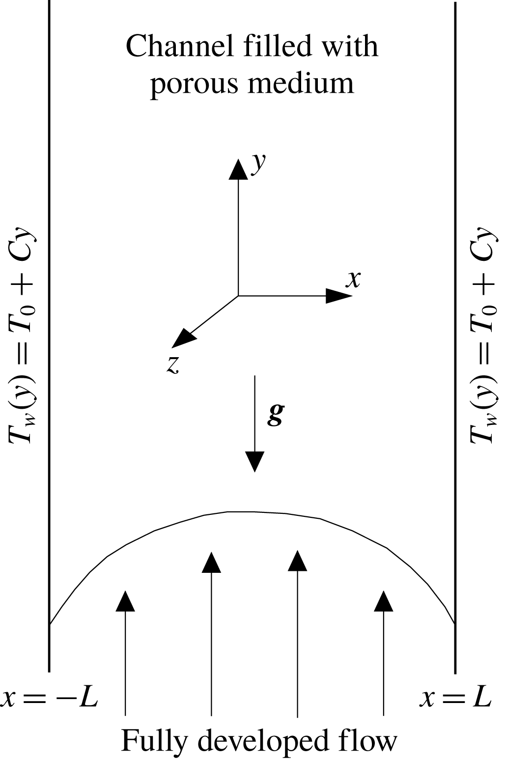
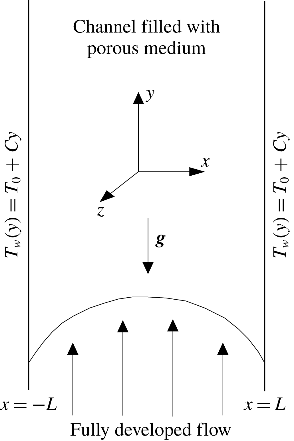
A pressure-driven non-isothermal flow in a vertical channel of width
 $2L$
filled with a porous medium is shown in figure 1. The wall temperature of the channel is assumed to vary linearly with
 $y$
as
 $T_{w}=T_{0}+Cy$
, where
 $C$
is a positive constant and
 $T_{0}$
is the upstream reference temperature. The gravitational force is aligned in the negative
 $y$
-direction. The medium is assumed to be homogeneous and isotropic in permeability. The convective flow through the porous medium is governed by a non-Darcy model. The heat transfer equation is written under the assumption of a local thermal equilibrium (LTE) state, i.e. the local temperatures of the fluid and solid phases are assumed to be identical. The thermo-physical properties of the fluid are assumed to be constant except for the density dependence of the buoyancy term in the momentum equation, which is satisfied by the Boussinesq approximation. Since the flows through the porous medium reveal inconsistencies in the usage of proper governing equations in the flow region, therefore a note on the considered model and consideration of the different terms in the momentum equation for the present problem is given in appendix A.
Schematic of the physical problem and coordinate system.
Following the discussion in above note, we consider non-Darcy volume averaged Navier–Stokes equations for the present theoretical investigation. The non-dimensionalized space coordinates
 $(x^{\ast },y^{\ast },z^{\ast })$
, dependent variables
 $(\boldsymbol{v}^{\ast },\unicode[STIX]{x1D703},P^{\ast })$
and time
 $t^{\ast }$
are calculated after scaling the dimensional variables as follows:
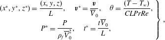 $$\begin{eqnarray}\displaystyle \left.\begin{array}{@{}c@{}}(x^{\ast },y^{\ast },z^{\ast })={\displaystyle \frac{(x,y,z)}{L}},\quad \boldsymbol{v}^{\ast }={\displaystyle \frac{\boldsymbol{v}}{\overline{V}_{0}}},\quad \unicode[STIX]{x1D703}={\displaystyle \frac{(T-T_{w})}{CLPrRe}},\\ P^{\ast }={\displaystyle \frac{P}{\unicode[STIX]{x1D70C}_{f}\overline{V}_{0}^{2}}},\quad t^{\ast }={\displaystyle \frac{t\overline{V}_{0}}{L}},\end{array}\!\right\}, & & \displaystyle\end{eqnarray}$$
where
 $\boldsymbol{v}^{\ast }=(u^{\ast },v^{\ast },w^{\ast })$
,
 $\unicode[STIX]{x1D703}$
,
 $P^{\ast }$
and
 $t^{\ast }$
are the dimensionless Darcy velocity vector, temperature, pressure and time, respectively. Furthermore,
 $\overline{V}_{0}$
is the dimensional average basic velocity and
 $\unicode[STIX]{x1D70C}_{f}$
is the fluid density. The dimensionless governing equations for continuity, momentum and energy, after dropping the asterisks, can be written as
 $$\begin{eqnarray}\displaystyle & \displaystyle \unicode[STIX]{x1D735}\boldsymbol{\cdot }\boldsymbol{v}=0, & \displaystyle\end{eqnarray}$$
 $$\begin{eqnarray}\displaystyle & \displaystyle \frac{1}{\unicode[STIX]{x1D700}}\frac{\unicode[STIX]{x2202}\boldsymbol{v}}{\unicode[STIX]{x2202}t}+\frac{1}{\unicode[STIX]{x1D700}^{2}}\boldsymbol{v}\boldsymbol{\cdot }\unicode[STIX]{x1D735}\boldsymbol{v}+F\boldsymbol{v}|\boldsymbol{v}|=-\unicode[STIX]{x1D735}P+\frac{Ra}{Re}\unicode[STIX]{x1D703}\boldsymbol{e}_{\boldsymbol{y}}+\frac{\unicode[STIX]{x1D706}}{Re}\unicode[STIX]{x1D6FB}^{2}\boldsymbol{v}-\frac{1}{DaRe}\boldsymbol{v}, & \displaystyle\end{eqnarray}$$
 $$\begin{eqnarray}\displaystyle & \displaystyle \unicode[STIX]{x1D70E}\frac{\unicode[STIX]{x2202}\unicode[STIX]{x1D703}}{\unicode[STIX]{x2202}t}+\boldsymbol{v}\boldsymbol{\cdot }\unicode[STIX]{x1D735}\unicode[STIX]{x1D703}=\frac{1}{RePr}(\unicode[STIX]{x1D6FB}^{2}\unicode[STIX]{x1D703}-v). & \displaystyle\end{eqnarray}$$
The dimensionless parameters appearing in the problem are the Rayleigh number
 $(Ra)$
, Reynolds number
 $(Re)$
, Prandtl number
 $(Pr)$
, Darcy number
 $(Da)$
, Forchheimer number
 $(F)$
and viscosity ratio (
 $\unicode[STIX]{x1D706}$
). They are defined as
 $$\begin{eqnarray}\displaystyle Ra=\frac{\text{g}\unicode[STIX]{x1D6FD}_{T}CL^{4}}{\unicode[STIX]{x1D708}k},\quad Re=\frac{\overline{V}_{0}L}{\unicode[STIX]{x1D708}},\quad Pr=\frac{\unicode[STIX]{x1D708}}{k},\quad Da=\frac{K}{L^{2}},\quad F=\frac{c_{F}L}{K^{1/2}}\quad \text{and}\quad \unicode[STIX]{x1D706}=\frac{\widetilde{\unicode[STIX]{x1D707}}}{\unicode[STIX]{x1D707}_{f}}, & & \displaystyle \nonumber\\ \displaystyle & & \displaystyle\end{eqnarray}$$
where
 $k$
is the thermal diffusivity,
 $\unicode[STIX]{x1D708}$
is the kinematic viscosity,
 $\unicode[STIX]{x1D6FD}_{T}$
is the thermal expansion coefficient,
 $\unicode[STIX]{x1D700}$
is the porosity of the medium,
 $c_{F}$
is the form drag coefficient,
 $K$
is the permeability of the porous medium,
 $g$
is gravitational acceleration,
 $\widetilde{\unicode[STIX]{x1D707}}$
is the effective viscosity,
 $\unicode[STIX]{x1D707}_{f}$
is the fluid viscosity and
 $\boldsymbol{e}_{\boldsymbol{y}}$
is the unit vector in the
 $y$
-direction. In (2.4),
 $\unicode[STIX]{x1D70E}$
denotes the ratio of the volumetric heat capacities of the medium and fluid.
3 Linear stability analysis
We assume that the flow is steady, unidirectional and fully developed, which gives rise to PMCF. Under these circumstances, the above governing equations (2.2)–(2.4) are reduced to a set of ordinary differential equations, which are defined in the operator form as
 $$\begin{eqnarray}\displaystyle & \displaystyle {\mathcal{L}}_{y}(V_{0},\unicode[STIX]{x1D6E9}_{0},Ra,Da,F^{\prime })=\unicode[STIX]{x1D706}\frac{\text{d}^{2}V_{0}}{\text{d}x^{2}}-\frac{1}{Da}V_{0}+Ra\unicode[STIX]{x1D6E9}_{0}-F^{\prime }|V_{0}|V_{0}=Re\frac{\text{d}P_{0}}{\text{d}y}, & \displaystyle\end{eqnarray}$$
 $$\begin{eqnarray}\displaystyle & \displaystyle {\mathcal{L}}(V_{0},\unicode[STIX]{x1D6E9}_{0})=\frac{\text{d}^{2}\unicode[STIX]{x1D6E9}_{0}}{\text{d}x^{2}}-V_{0}=0, & \displaystyle\end{eqnarray}$$
with boundary conditions
 $$\begin{eqnarray}\displaystyle V_{0}=\unicode[STIX]{x1D6E9}_{0}=0\quad \text{at}~x=\pm 1, & & \displaystyle\end{eqnarray}$$
where
 $V_{0}$
,
 $\unicode[STIX]{x1D6E9}_{0}$
and
 $P_{0}$
are the basic state velocity, basic state temperature and basic state pressure, respectively and
 $F^{\prime }=FRe$
. Note that the wall bounded channel is filled with a highly permeable porous medium that has a high porosity, consequently the fully developed flow has to satisfy the above no-slip condition at the walls. The quantity
 $Re(\text{d}P_{0}/\text{d}y)$
is determined by use of the global mass conservation:
 $$\begin{eqnarray}\displaystyle \int _{-1}^{1}V_{0}\,\text{d}x=2. & & \displaystyle\end{eqnarray}$$
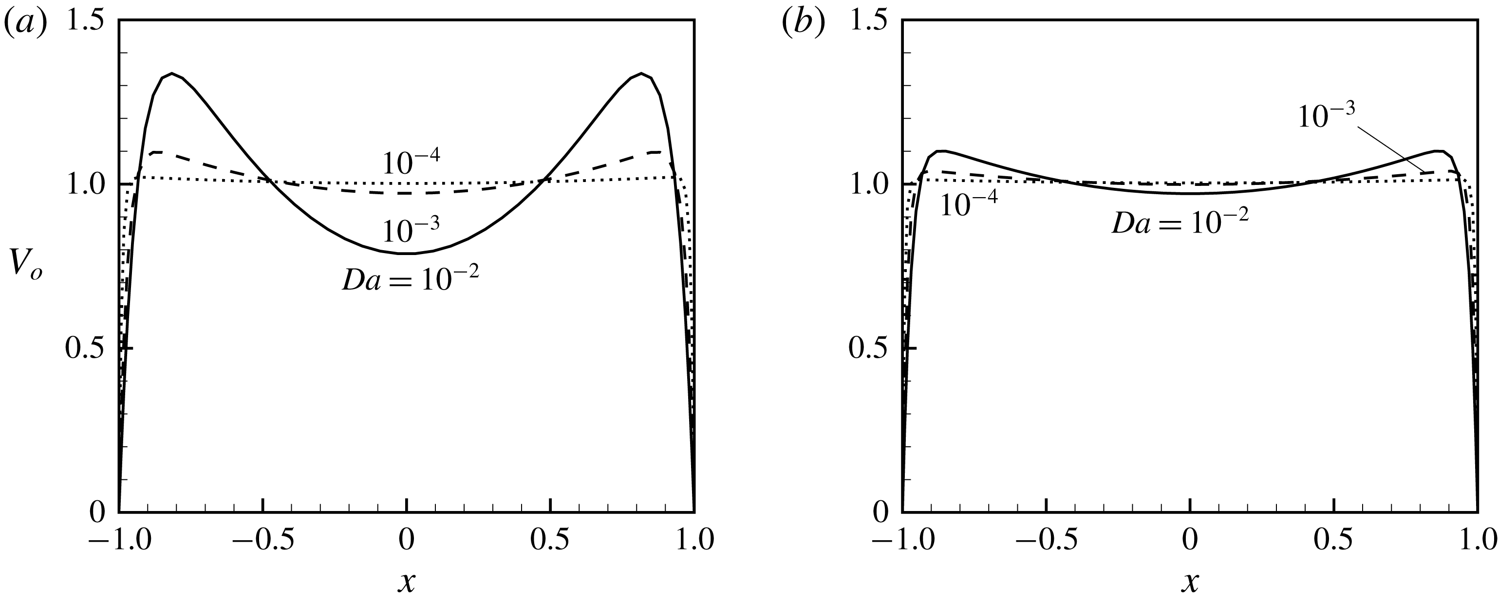
The velocity profile contains points of inflection, which suggests the potential for instability. However, these points of inflection in the velocity profile shift towards the walls on decreasing the medium’s permeability (see figure 18 in appendix B.1).
To investigate the stability of the above basic flow, the classical normal mode analysis (Drazin & Reid Reference Drazin and Reid2004) is used. The dependent variables are decomposed into a basic state and infinitesimal disturbances. The velocity vector, temperature and pressure are written as
 $$\begin{eqnarray}\displaystyle \boldsymbol{v}=V_{0}(x)\boldsymbol{e}_{\boldsymbol{y}}+\boldsymbol{v}^{\prime },\quad \unicode[STIX]{x1D703}=\unicode[STIX]{x1D6E9}_{0}(x)+\unicode[STIX]{x1D703}^{\prime },\quad P=P_{0}(y)+p^{\prime }. & & \displaystyle\end{eqnarray}$$
These infinitesimal disturbances of the corresponding field variables are separated into normal mode form as
 $$\begin{eqnarray}\displaystyle (\boldsymbol{v}^{\prime },\unicode[STIX]{x1D703}^{\prime },p^{\prime })^{\text{T}}=\text{e}^{\text{i}(\unicode[STIX]{x1D6FC}y+\unicode[STIX]{x1D6FD}z-\unicode[STIX]{x1D6FC}ct)}(\hat{\boldsymbol{v}},\hat{\unicode[STIX]{x1D703}}(x),\hat{p}(x))^{\text{T}}, & & \displaystyle\end{eqnarray}$$
where
 $\unicode[STIX]{x1D6FC}$
and
 $\unicode[STIX]{x1D6FD}$
are the wavenumbers in the streamwise (
 $y$
) and spanwise (
 $z$
) directions, respectively, and
 $c=c_{r}+\text{i}c_{i}$
is a complex wave speed. The growth or decay of the disturbance is determined from the sign of
 $c_{i}$
. The flow is stable or neutrally stable or unstable accordingly as
 $c_{i}<0$
or
 $c_{i}=0$
or
 $c_{i}>0$
, respectively. On substituting (3.5) and (3.6) into the governing equations (2.2)–(2.4), the linearized disturbance equations obtained in operator form are given in appendix C.1.
The corresponding boundary conditions for the perturbed field variables are
 $$\begin{eqnarray}\displaystyle \hat{u} =\hat{v}={\hat{w}}=\hat{\unicode[STIX]{x1D703}}=0\quad \text{at}~x=\pm 1. & & \displaystyle\end{eqnarray}$$
The linear disturbance equations (C 1)–(C 5) are solved by eliminating the pressure terms along with the no-slip and impermeability condition of velocity and zero temperature perturbation on the walls. These linear disturbance equations along with the boundary conditions form a generalized eigenvalue problem for a complex disturbance wave speed (
 $c$
), which is given as
 $$\begin{eqnarray}\displaystyle \unicode[STIX]{x1D63C}X=c\unicode[STIX]{x1D63D}X, & & \displaystyle\end{eqnarray}$$
where
 $X=[\hat{u} ,\hat{v},{\hat{w}},\hat{\unicode[STIX]{x1D703}}]^{\text{T}}$
is the representation of the eigenfunction, and
 $\unicode[STIX]{x1D63C}$
and
 $\unicode[STIX]{x1D63D}$
are square complex matrices. If
 $X$
is an eigenfunction related to the least stable eigenvalue at some critical point then
 $X\text{e}^{[\text{i}\unicode[STIX]{x1D6FC}(y-c_{r}t)+\text{i}\unicode[STIX]{x1D6FD}z]}$
is defined as the fundamental disturbance where
 $c_{r}$
is the corresponding wave speed. The fundamental disturbance will be used frequently in different parts of the weakly nonlinear analysis.
The linear stability theory is used to find the location of the bifurcation point or critical point (
 $\unicode[STIX]{x1D6FC},Ra$
) and to predict the form of the developing disturbances. It does not provide any information about the actual size of the disturbances (amplitude) away from the critical value. To analyse the amplitude of such disturbances, a weakly nonlinear stability analysis is required. The results of the linear stability analysis are also required to carry out a nonlinear analysis. Therefore, a brief review of linear stability results is presented below. It is important to mention here that, although the problem in this paper is that of heated upward flow in a vertical channel, the results may also be used for a cooled downward flow in a vertical channel and vice versa. This is because the equations governing heated (cooled) upward flow are identical to those of cooled (heated) downward flow.
3.1 Review of linear stability results
The linear stability analysis of the present problem has been studied by a number of authors (Bera & Khalili Reference Bera and Khalili2002; Chen Reference Chen2004; Kumar et al.
Reference Kumar, Bera and Khalili2010) in the literature. In these studies, the rigorous numerical study of different controlling parameters, as well as the impact of drag forces and inertia on the stability of the PMCF, was carried out. The problem contains eight important parameters such as Reynolds number
 $(Re)$
, Rayleigh number
 $(Ra)$
, Darcy number
 $(Da)$
, Prandtl number
 $(Pr)$
, Forchheimer number (
 $F$
), porosity
 $(\unicode[STIX]{x1D700})$
, viscosity ratio
 $(\unicode[STIX]{x1D706})$
and heat capacity ratio
 $(\unicode[STIX]{x1D70E})$
. The objective of the present study is to investigate the influence of the nonlinear interaction of different harmonic modes on the instability of flow through a highly permeable porous medium. For this, two fluids, air (
 $Pr=0.7$
) and water (
 $Pr=7$
), are chosen. Apart from this, to avoid too many parametric studies, we have fixed certain parameters for the present study. The porosity, viscosity ratio and heat capacity ratio are kept constant at 0.9, 1 and 1, respectively. Here, three different values (
 $10^{-2},10^{-3}$
and
 $10^{-4}$
) of
 $Da$
and three different values (0.0006, 0.006 and 0.06) of
 $c_{F}$
are taken to examine the present problem. There is a lack of experimental data on the value of
 $c_{F}$
related to a non-isothermal system, so the consideration of the above three values of
 $c_{F}$
is based on the information mentioned in Calmidi & Mahajan (Reference Calmidi and Mahajan2000) that the value of
 $c_{F}$
can be as small as or less than 0.1 (for metallic foam).
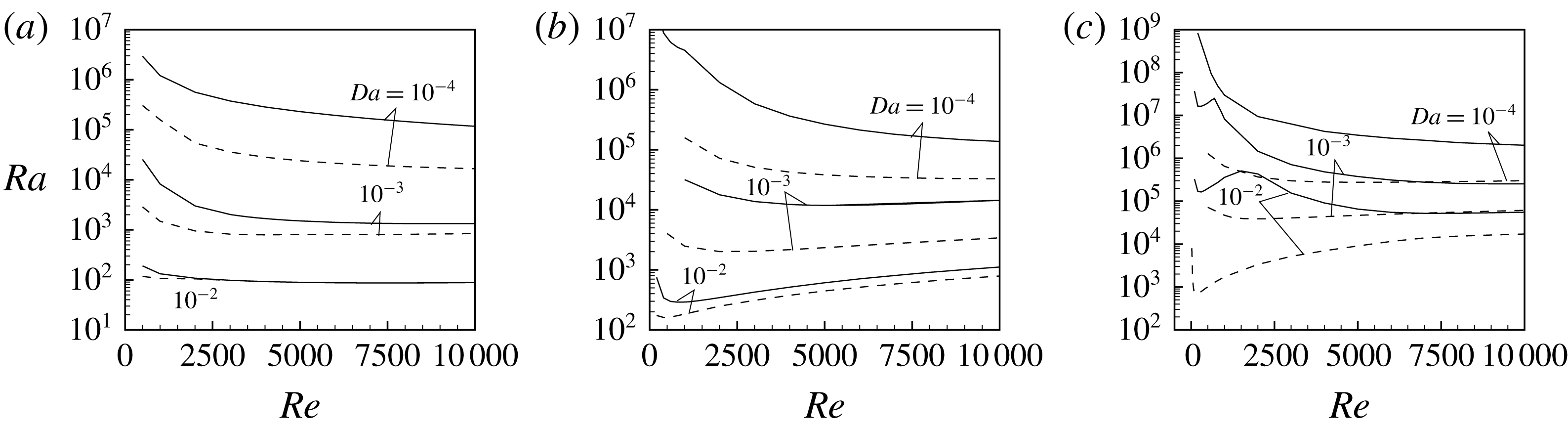
Linear stability boundaries in the (
 $Re,Ra$
)-plane: (a)
 $c_{F}=6\times 10^{-4}$
, (b)
 $c_{F}$
 $=$
 $6\times 10^{-3}$
and (c)
 $c_{F}=6\times 10^{-2}$
, where the solid line is
 $Pr=0.7$
and the dashed line is
 $Pr=7$
.
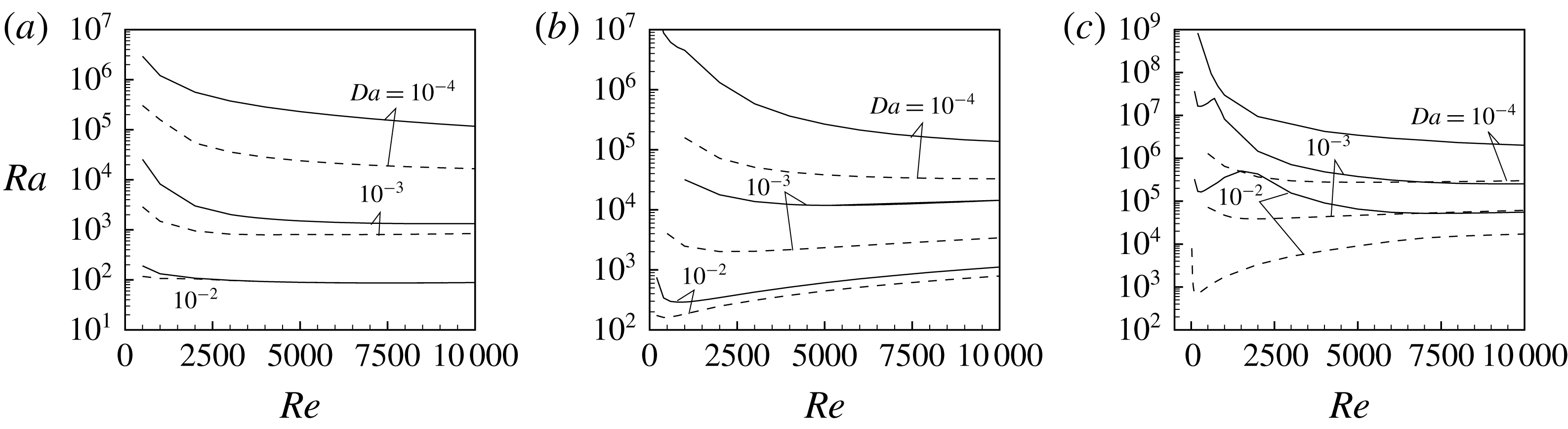
We present the linear stability results for air (
 $Pr=0.7$
) and water (
 $Pr=7$
) in the
 $(Re,Ra)$
-plane. The linear stability boundaries for three values, 0.0006, 0.006 and 0.06, of
 $c_{F}$
are plotted in figures 2(a), 2(b) and 2(c), respectively. Here, in general, based on the value of
 $c_{F}$
,
 $Pr$
and
 $Da$
the instability boundary curve first decreases on increasing the value of
 $Re$
and may reach a minimum value of
 $Re$
, above which the curve will have an increasing characteristic. This may continue further to a certain range of
 $Re$
and beyond such that it may asymptotically converge to a constant. The typical decreasing characteristic of the instability curve up to a minimum value of
 $Re$
is a consequence of the following fact. In general, the shear force induced by increasing
 $Re$
destabilizes the flow. Also, in a porous medium, increasing
 $Re$
increases the form drag induced in the flow which has a stabilizing characteristic. As mentioned in Bera & Khalili (Reference Bera and Khalili2002), under the present heating condition, a slow flow can carry denser fluid upward into the region of lighter fluid. While doing so, in addition to the energy due to the shear force existing in a viscous fluid, for a porous medium, two new disturbance energies with stabilizing characteristics, namely the one caused by surface drag associated with the Darcy term and the other caused by the form drag associated with the Forchheimer term, appear in the region of high velocity. However, the contribution of form drag may be very small for such types of flow. As a consequence, a point of inflection develops, leading to a local high shear layer. In this situation, a small enhancement of
 $Re$
makes the convection in the direction of the main flow stronger, and more dense fluid can be transported upwards to destabilize the flow, and hence the critical heating condition (i.e. critical
 $Ra$
) falls drastically. As
 $Re$
is increased further, the induced form drag may take a dominant role and this results in an increased critical heating condition.
Furthermore, when
 $c_{F}=6\times 10^{-3}$
is replaced by
 $c_{F}=6\times 10^{-2}$
, figure 2(c) shows that, in an air-saturated porous medium, based on the value of
 $Da$
, there exists a threshold value of
 $Re$
(e.g.
 $Re=2000$
for
 $Da=10^{-2}$
and
 $Re=700$
for
 $Da=10^{-3}$
) beyond which the instability curve decreases smoothly as a function of
 $Re$
. However, in the range
 $0<Re\leqslant Re$
, the (threshold) instability boundary curve first decreases up to a minimum value of
 $Re$
and then increases, which may be the consequence of the sizeable constant value of
 $c_{F}$
even in the Darcy regime. As compared to the PMCF of air, the same for water is much more unstable. The instability boundaries show a more stable flow with decreasing medium permeability. Apart from these, the induced form drag in the system delays the instability of the flow.
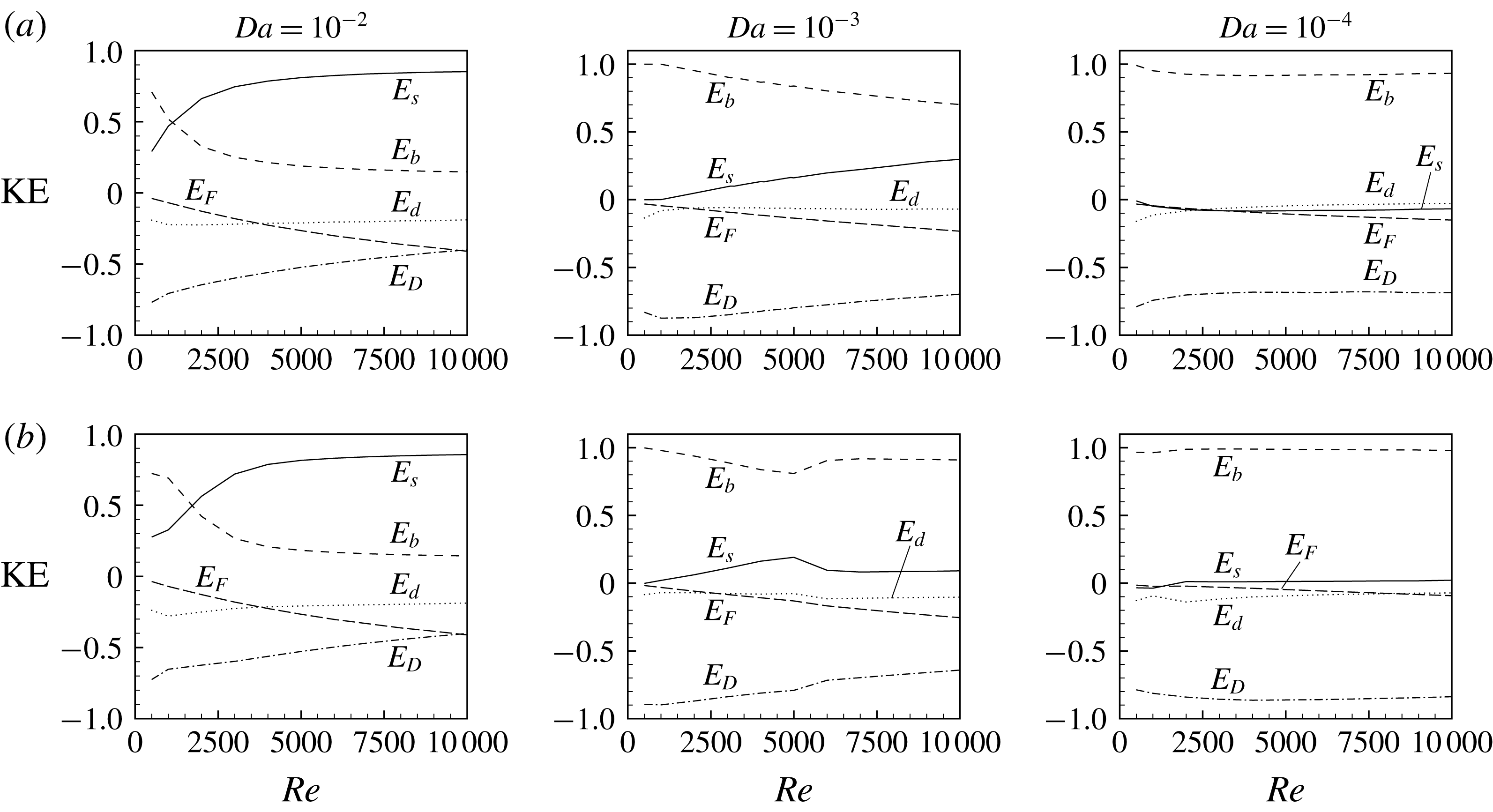
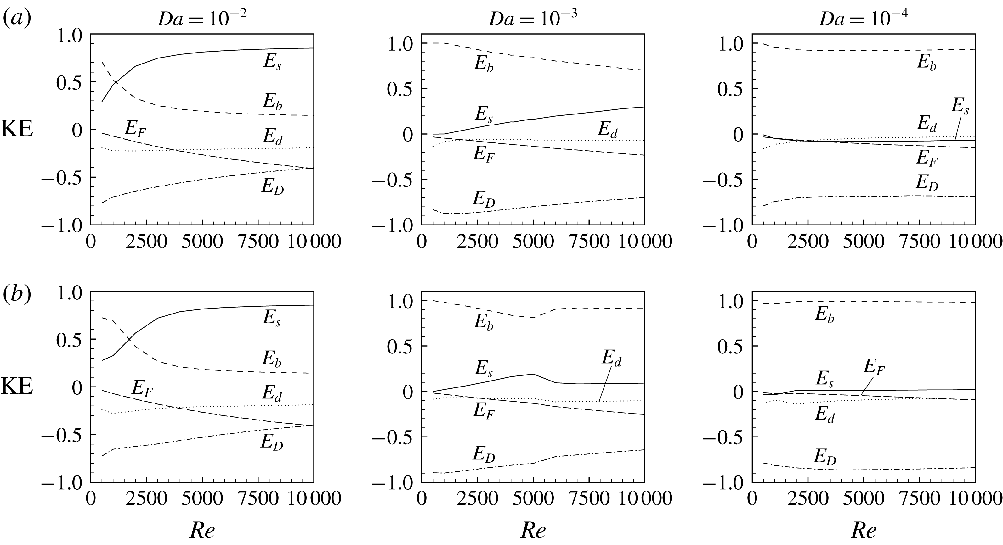
The disturbance kinetic energy (KE) balance corresponding to a neutral stability curve also provides some insight into the transport mechanisms during the flow instability. The mathematical details of the balance of KE can be seen in the paper by Bera & Khalili (Reference Bera and Khalili2006). The different energy terms of the KE balance for
 $c_{F}=6\times 10^{-4}$
are shown in figures 3(a) and 3(b) for air and water, respectively. Due to the similarity, the KE spectra for all other considered values of
 $c_{F}$
are not shown here. As can be seen from figure 3(a,b), based on the permeability of the medium considered, the type of instability may be buoyant (or thermal–buoyant), mixed (or interactive) and shear (or thermal–shear). Here, the type of instability is defined on the basis of the contribution to energy production (or, destruction) of the shear term (
 $E_{s}$
) and the buoyant term (
 $E_{b}$
). If, in the energy balance, the contribution of
 $E_{s}$
(
 $E_{b}$
) is more than or equal to 75 % then the type of instability is defined as shear (buoyant), otherwise it is defined as mixed. Thus, the mixed mode of instability is defined as 25 %–75 % contribution to the total KE production by both buoyant and convective terms. The kinetic energy production for
 $Da=10^{-2}$
, when the fluid is air (water), shows three different types of instability: buoyant for
 $Re\leqslant 500$
(
 $Re\leqslant 500$
), mixed for
 $500<Re\leqslant 3150$
(
 $500<Re\leqslant 3460$
) and shear for
 $Re>3150$
(
 $Re>3460$
). Similarly, for
 $Da=10^{-3}$
, it shows two types of instability: buoyant for
 $Re\leqslant 8000$
and mixed for
 $Re>8000$
in the case of air, whereas for water only the buoyant type occurs. For air as well as water, when
 $Da=10^{-4}$
, KE production due to the buoyant term remains prominent in the entire range of
 $Re$
considered in this study, consequently, buoyant instability is the only type of instability. Note that for
 $Da$
equal to
 $10^{-3}$
or
 $10^{-4}$
KE production or destruction is mainly balanced by dissipation of KE due to surface drag (
 $E_{D}$
). However, for
 $Da=10^{-2}$
it is different. Here, dissipation of KE is made through
 $E_{D}$
as well as
 $E_{F}$
.
Linear disturbance kinetic energy (KE) balance at the critical level: (a)
 $Pr=0.7$
and (b)
 $Pr=7$
when
 $c_{F}=6\times 10^{-4}$
.
It has been also found that when
 $c_{F}=6\times 10^{-4}$
is replaced by
 $c_{F}=6\times 10^{-3}$
, in general, whether the porous medium is saturated by air or water, the type of instability is buoyant and energy production due to the buoyant term is balanced by dissipation of KE through the surface as well as form drag (figure is not shown here). For
 $Re>1100$
,
 $Da=10^{-2}$
and
 $Pr=0.7$
the mode of instability is of mixed type, i.e. both
 $E_{s}$
and
 $E_{b}$
are positive and take active roles in the KE balance. It is also worth mentioning here that, in an air-saturated porous medium for
 $Da=10^{-3}$
or
 $Da=10^{-4}$
,
 $E_{s}$
is negative (i.e. energy is lost to basic flow, and is in favour of stabilizing the flow).
The occurrence of instability in a flow may lead to the replacement of the original laminar flow by a new laminar flow due to the superimposition of finite disturbances. This flow may be expected to persist for a certain range of Rayleigh numbers beyond the critical value and then become unstable at some new Rayleigh number against a new (second) type of disturbance. A new equilibrium flow, consisting of a mean flow with two superimposed harmonics, is then conceivable for a range of Rayleigh numbers above the second critical value. In a purely fluid domain, as the Rayleigh number is increased further, additional modes of disturbance may appear successively until turbulence is achieved. In this way, a sequence of instabilities may exist before it leads finally to turbulence (Hof et al. Reference Hof, van Doorne, Westerweel, Nieuwstadt, Faisst, Eckhardt, Wedin, Kerswell and Waleffe2004). Since turbulent flow in a wall bounded porous medium is possible (Jin & Kuznetsov Reference Jin and Kuznetsov2017), therefore, the above similar phenomena may be expected in fluid flow through highly permeable porous media. Thus, a nonlinear stability analysis is necessary to study the structure of the flow field that results from linear stability analysis.
4 Formulation of finite amplitude equations
In the present article the amplitude expansions are given based on the analysis of Stuart (Reference Stuart1960) and Yao & Rogers (Reference Yao and Rogers1992). The Fourier expansion of the
 $y$
-direction velocity component in separable form is
 $$\begin{eqnarray}\displaystyle v(x,y,z,t) & = & \displaystyle V(x,\unicode[STIX]{x1D70F})E^{0}+\hat{v}_{1}(x,\unicode[STIX]{x1D70F})E^{1}+\hat{v}_{2}(x,\unicode[STIX]{x1D70F})E^{2}+\cdots +\text{c.c.}\nonumber\\ \displaystyle & = & \displaystyle E^{0}[V_{0}(x)+c_{i}|B(\unicode[STIX]{x1D70F})|^{2}V_{1}(x)+O((c_{i})^{2})]\nonumber\\ \displaystyle & & \displaystyle +\,E^{1}[(c_{i})^{1/2}Bv_{10}+(c_{i})^{3/2}B|B|^{2}v_{11}+O((c_{i})^{5/2})]\nonumber\\ \displaystyle & & \displaystyle +\,E^{2}[c_{i}B^{2}v_{20}+O((c_{i})^{2})]+\cdots +\text{c.c.},\end{eqnarray}$$
where
 $E^{j}=\text{e}^{j[\text{i}\unicode[STIX]{x1D6FC}(y-c_{r}t)+\text{i}\unicode[STIX]{x1D6FD}z]}$
,
 $j=0,1,2$
;
 $\unicode[STIX]{x1D6FC}$
is the wavenumber corresponding to the critical
 $Ra$
, and
 $c_{r}$
is the real part of the wave speed of the most unstable disturbance wave.
 $B$
denotes an amplitude function, which will be calculated from the Landau equation, and c.c. stands for complex conjugate.
The method of multiple time scales is used to derive an evolution equation for slowly varying amplitude. Two types of time scales (a fast time scale (
 $t$
) and slow time scale
 $(\unicode[STIX]{x1D70F})$
) are used in the nonlinear stability analysis of the flow. The choice of the fast time scale is associated with the exponential development of the disturbance as in the linear stability analysis. The nonlinear terms become important when the disturbance attains a finite amplitude. In this situation, the temporal behaviour of the disturbance deviates from exponential behaviour. This is characterized by another time scale (the slow time scale). The slow time scale leads to stages when the growth/decay of the disturbances is affected by nonlinearities of different order. The slow time scale
 $\unicode[STIX]{x1D70F}=c_{i}t$
modifies the time derivative as
 $$\begin{eqnarray}\displaystyle \frac{\unicode[STIX]{x2202}}{\unicode[STIX]{x2202}t}\rightarrow \frac{\unicode[STIX]{x2202}}{\unicode[STIX]{x2202}t}+c_{i}\frac{\unicode[STIX]{x2202}}{\unicode[STIX]{x2202}\unicode[STIX]{x1D70F}}. & & \displaystyle\end{eqnarray}$$
The multiple time scale approach is valid when the amplitude dynamics changes substantially as the disturbance develops. Similarly, we can write the expansions for the other dependent variables in terms of
 $c_{i}$
and the amplitude function
 $(B)$
. The mathematical justification of the perturbation expansion is as follows.
It is well known from the linear stability analysis that
 $c_{i}$
is proportional to the difference between the actual and critical Rayleigh numbers (or Reynolds numbers)
 $\unicode[STIX]{x1D6E5}$
. Yao & Rogers (Reference Yao and Rogers1992) have shown that the square of the equilibrium amplitude (to be discussed later) is proportional to
 $\unicode[STIX]{x1D6E5}$
. Consequently, the equilibrium amplitude is proportional to
 $(c_{i})^{1/2}$
. Hence, in an
 $\unicode[STIX]{x1D6FC}$
disturbance the amplitude of
 $\hat{v}_{1}$
is of order
 $(c_{i})^{1/2}$
. Field variables that are expanded in higher wavenumbers are scaled according to the number of nonlinear interactions it takes to generate them. For example,
 $2\unicode[STIX]{x1D6FC}$
disturbances require the interaction of two
 $\unicode[STIX]{x1D6FC}$
-perturbations, thus the amplitude of
 $\hat{v}_{2}$
is of order
 $(c_{i})^{1}$
. We also assume that
 $\unicode[STIX]{x2202}/\unicode[STIX]{x2202}t$
is never of greater magnitude than
 $c_{i}$
, which is its order of magnitude according to the linear theory. The distortion of the mean flow
 $(V)$
is of order
 $c_{i}$
, which arises from part of the Reynolds stress (Stewartson & Stuart Reference Stewartson and Stuart1971).
4.1 Derivation of cubic Landau equation
On substituting equation (4.1) into the governing equations (2.2)–(2.4) and separating the harmonic components, the equations for the harmonic
 $E^{0}$
are
 $$\begin{eqnarray}\displaystyle & & \displaystyle {\mathcal{L}}_{y}(V_{0},\unicode[STIX]{x1D6E9}_{0},Ra,Da,F,Re)-Re\frac{\text{d}P_{0}}{\text{d}y}+c_{i}|B|^{2}\left\{\unicode[STIX]{x1D706}\frac{\text{d}^{2}V_{1}}{\text{d}x^{2}}-\frac{1}{Da}V_{1}+Ra\unicode[STIX]{x1D6E9}_{1}-2F^{\prime }|V_{0}|V_{1}\right.\nonumber\\ \displaystyle & & \displaystyle \quad -\left.Re\frac{\text{d}P_{1}}{\text{d}y}-\frac{Re}{\unicode[STIX]{x1D700}^{2}}\left[\frac{\text{d}}{\text{d}x}(\tilde{v}_{10}u_{10}+v_{10}\tilde{u} _{10})\right]\!\right\}=O((c_{i})^{2}),\end{eqnarray}$$
 $$\begin{eqnarray}\displaystyle {\mathcal{L}}(V_{0},\unicode[STIX]{x1D6E9}_{0})+c_{i}|B|^{2}\left\{{\mathcal{L}}(V_{1},\unicode[STIX]{x1D6E9}_{1})-RePr\left[\frac{\text{d}}{\text{d}x}(\tilde{u} _{10}\unicode[STIX]{x1D703}_{10}+u_{10}\tilde{\unicode[STIX]{x1D703}}_{10})\right]\!\right\}=O((c_{i})^{2}). & & \displaystyle\end{eqnarray}$$
Similarly, the equations for the harmonic
 $E^{1}$
are
 $$\begin{eqnarray}\displaystyle (c_{i})^{1/2}B\{\mathscr{L}_{o}(\unicode[STIX]{x1D6FC},\unicode[STIX]{x1D6FD},u_{10},v_{10},w_{10})\}+(c_{i})^{3/2}B|B|^{2}\{\mathscr{L}_{o}(\unicode[STIX]{x1D6FC},\unicode[STIX]{x1D6FD},u_{11},v_{11},w_{11})\}=O(c_{i}^{5/2}), & & \displaystyle\end{eqnarray}$$
 $$\begin{eqnarray}\displaystyle & & \displaystyle (c_{i})^{1/2}B\{\mathscr{L}_{x}(\unicode[STIX]{x1D6FC},\unicode[STIX]{x1D6FD},c,u_{10},p_{10},V_{0},Da,F,Re)\}\nonumber\\ \displaystyle & & \displaystyle \quad +\,(c_{i})^{3/2}\left\{B|B|^{2}\mathscr{L}_{x}(\unicode[STIX]{x1D6FC},\unicode[STIX]{x1D6FD},c,u_{11},p_{11},V_{0},Da,F,Re)\right.\nonumber\\ \displaystyle & & \displaystyle \quad -\left.B|B|^{2}{\mathcal{G}}_{x}+\frac{Re}{\unicode[STIX]{x1D700}}\frac{\text{d}B}{\text{d}\unicode[STIX]{x1D70F}}u_{10}-\frac{\unicode[STIX]{x1D6FC}BRe}{\unicode[STIX]{x1D700}}u_{10}\right\}=O(c_{i}^{5/2}),\end{eqnarray}$$
 $$\begin{eqnarray}\displaystyle & & \displaystyle (c_{i})^{1/2}B\{\mathscr{L}_{y}(\unicode[STIX]{x1D6FC},\unicode[STIX]{x1D6FD},c,u_{10},v_{10},p_{10},\unicode[STIX]{x1D703}_{10},V_{0},Ra,Da,F,Re)\}\nonumber\\ \displaystyle & & \displaystyle \quad +\,(c_{i})^{3/2}\left\{B|B|^{2}\mathscr{L}_{y}(\unicode[STIX]{x1D6FC},\unicode[STIX]{x1D6FD},c,u_{11},v_{11},p_{11},\unicode[STIX]{x1D703}_{11},V_{0},Ra,Da,F,Re)\right.\nonumber\\ \displaystyle & & \displaystyle \quad -\left.B|B|^{2}{\mathcal{G}}_{y}+\frac{Re}{\unicode[STIX]{x1D700}}\frac{\text{d}B}{\text{d}\unicode[STIX]{x1D70F}}v_{10}-\frac{\unicode[STIX]{x1D6FC}BRe}{\unicode[STIX]{x1D700}}v_{10}\right\}=O((c_{i})^{5/2}),\end{eqnarray}$$
 $$\begin{eqnarray}\displaystyle & & \displaystyle (c_{i})^{1/2}B\{\mathscr{L}_{z}(\unicode[STIX]{x1D6FC},\unicode[STIX]{x1D6FD},c,w_{10},p_{10},V_{0},Da,F,Re)\}\nonumber\\ \displaystyle & & \displaystyle \quad +\,(c_{i})^{3/2}\left\{B|B|^{2}\mathscr{L}_{z}(\unicode[STIX]{x1D6FC},\unicode[STIX]{x1D6FD},c,w_{11},p_{11},V_{0},Da,F,Re)\right.\nonumber\\ \displaystyle & & \displaystyle \quad -\left.B|B|^{2}{\mathcal{G}}_{z}+\frac{Re}{\unicode[STIX]{x1D700}}\frac{\text{d}B}{\text{d}\unicode[STIX]{x1D70F}}w_{10}-\frac{\unicode[STIX]{x1D6FC}BRe}{\unicode[STIX]{x1D700}}w_{10}\right\}=O((c_{i})^{5/2}),\end{eqnarray}$$
 $$\begin{eqnarray}\displaystyle & & \displaystyle (c_{i})^{1/2}B\{\mathscr{L}(\unicode[STIX]{x1D6FC},\unicode[STIX]{x1D6FD},c,u_{10},v_{10},\unicode[STIX]{x1D703}_{10},V_{0},\unicode[STIX]{x1D6E9}_{0})\}\nonumber\\ \displaystyle & & \displaystyle \quad +\,(c_{i})^{3/2}\left\{B|B|^{2}\mathscr{L}(\unicode[STIX]{x1D6FC},\unicode[STIX]{x1D6FD},c,u_{11},v_{11},\unicode[STIX]{x1D703}_{11},V_{0},\unicode[STIX]{x1D6E9}_{0})\right.\nonumber\\ \displaystyle & & \displaystyle \quad -\left.B|B|^{2}{\mathcal{G}}-RePr\left(\frac{\text{d}B}{\text{d}\unicode[STIX]{x1D70F}}\unicode[STIX]{x1D703}_{10}-\unicode[STIX]{x1D6FC}B\unicode[STIX]{x1D703}_{10}\right)\!\right\}=O((c_{i})^{5/2}),\end{eqnarray}$$
where the
 ${\mathcal{G}}$
values are defined in appendix C.2.
The equations for the harmonic
 $E^{2}$
are
 $$\begin{eqnarray}\displaystyle c_{i}B^{2}\{\mathscr{L}_{o}(2\unicode[STIX]{x1D6FC},2\unicode[STIX]{x1D6FD},u_{20},v_{20},w_{20})\}=O((c_{i})^{2}), & & \displaystyle\end{eqnarray}$$
 $$\begin{eqnarray}\displaystyle & & \displaystyle c_{i}B^{2}\left\{\!\mathscr{L}_{x}(2\unicode[STIX]{x1D6FC},2\unicode[STIX]{x1D6FD},c,u_{20},p_{20},V_{0},Da,F,Re)+\frac{Re}{\unicode[STIX]{x1D700}^{2}}\left(\text{i}\unicode[STIX]{x1D6FC}u_{10}v_{10}+u_{10}\frac{\text{d}u_{10}}{\text{d}x}+\text{i}\unicode[STIX]{x1D6FD}u_{10}w_{10}\right)\!\right\}\nonumber\\ \displaystyle & & \displaystyle \quad =O((c_{i})^{2}),\end{eqnarray}$$
 $$\begin{eqnarray}\displaystyle & & \displaystyle c_{i}B^{2}\left\{\mathscr{L}_{y}(2\unicode[STIX]{x1D6FC},2\unicode[STIX]{x1D6FD},c,u_{20},v_{20},p_{20},\unicode[STIX]{x1D703}_{20},V_{0},Ra,Da,F,Re)\right.\nonumber\\ \displaystyle & & \displaystyle \qquad +\left.\frac{Re}{\unicode[STIX]{x1D700}^{2}}\left(\text{i}\unicode[STIX]{x1D6FC}v_{10}^{2}+u_{10}\frac{\text{d}v_{10}}{\text{d}x}+\text{i}\unicode[STIX]{x1D6FD}v_{10}w_{10}\right)\!\right\}\nonumber\\ \displaystyle & & \displaystyle \quad =O((c_{i})^{2}),\end{eqnarray}$$
 $$\begin{eqnarray}\displaystyle & & \displaystyle c_{i}B^{2}\left\{\mathscr{L}_{z}(2\unicode[STIX]{x1D6FC},2\unicode[STIX]{x1D6FD},c,w_{20},p_{20},V_{0},Da,F,Re)+\frac{Re}{\unicode[STIX]{x1D700}^{2}}\left(\text{i}\unicode[STIX]{x1D6FC}v_{10}w_{10}+u_{10}\frac{\text{d}w_{10}}{\text{d}x}+\text{i}\unicode[STIX]{x1D6FD}w_{10}^{2}\right)\!\right\}\nonumber\\ \displaystyle & & \displaystyle \quad =O((c_{i})^{2}),\end{eqnarray}$$
 $$\begin{eqnarray}\displaystyle & & \displaystyle c_{i}B^{2}\left\{\mathscr{L}(2\unicode[STIX]{x1D6FC},2\unicode[STIX]{x1D6FD},c,u_{20},v_{20},\unicode[STIX]{x1D703}_{20},V_{0},\unicode[STIX]{x1D6E9}_{0})-RePr\left(\text{i}\unicode[STIX]{x1D6FC}v_{10}\unicode[STIX]{x1D703}_{10}+u_{10}\frac{\text{d}\unicode[STIX]{x1D703}_{10}}{\text{d}x}+\text{i}\unicode[STIX]{x1D6FD}w_{10}\unicode[STIX]{x1D703}_{10}\right)\!\right\}\nonumber\\ \displaystyle & & \displaystyle \quad =O((c_{i})^{2}).\end{eqnarray}$$
Here
 ${\sim}$
denotes the complex conjugate. Consideration of higher-order harmonics (
 $E^{3},E^{4}$
, etc.) in (4.1) is not necessary to obtain the first Landau coefficient. Therefore, these terms are not included in the series.
The system of harmonic equations (4.3)–(4.14) can be solved sequentially in increasing power of
 $c_{i}$
. At order
 $(c_{i})^{0}$
, the harmonic
 $E^{0}$
contains exactly the same basic state equations (3.1)–(3.2). The unknown functions
 $V_{0}$
and
 $\unicode[STIX]{x1D6E9}_{0}$
are obtained from (3.1), (3.2). At order
 $(c_{i})^{1/2}$
, the harmonic
 $E^{1}$
contains linear stability equations and the contribution of other harmonics (
 $E^{0}$
and
 $E^{2}$
) is zero. The functions
 $u_{10}$
,
 $v_{10}$
,
 $w_{10}$
and
 $\unicode[STIX]{x1D703}_{10}$
are given by the eigenfunctions of the linear stability equations at a particular wavenumber as well as
 $Ra$
. At order
 $(c_{i})^{1}$
, the harmonics
 $E^{0}$
and
 $E^{2}$
produce the non-homogeneous equations for the basic flow distortion functions
 $V_{1}$
and
 $\unicode[STIX]{x1D6E9}_{1}$
as well as for the functions
 $u_{20}$
,
 $v_{20}$
,
 $w_{20}$
and
 $\unicode[STIX]{x1D703}_{20}$
, respectively. The non-homogeneous part of these equations contains the known variables
 $u_{10}$
,
 $v_{10}$
,
 $w_{10}$
,
 $\unicode[STIX]{x1D703}_{10}$
and their derivatives, which are calculated from a lower-order analysis. At order
 $(c_{i})^{3/2}$
, the equations of harmonic
 $E^{1}$
become non-homogeneous. The left-hand sides of these equations contain linear stability operators operating on
 $u_{11}$
,
 $v_{11}$
,
 $w_{11}$
,
 $\unicode[STIX]{x1D703}_{11}$
and
 $p_{11}$
, whereas the right-hand sides of these equations contain the terms proportional to
 $\text{d}B/\text{d}\unicode[STIX]{x1D70F}$
,
 $B$
and
 $B|B|^{2}$
. The coefficients of these terms on the right-hand sides are known from the lower-order analysis. The homogeneous form of the equations of
 $E^{1}$
is the same as for the linear stability equations. For a non-trivial solution of the
 $E^{1}$
equations, the integrability condition can be used to determine the unknown amplitude function
 $B$
. In order to formulate the integrability condition, the solution of a homogeneous adjoint system corresponding to the linear stability problem (see appendix C) is required. Therefore, the right-hand sides of the non-homogeneous equations of
 $E^{1}$
at order
 $(c_{i})^{3/2}$
must be orthogonal to the adjoint field variables. In this manner, multiplying the above right-hand side terms by the adjoint field variables
 $p^{\ast }$
,
 $u^{\ast }$
,
 $v^{\ast }$
,
 $w^{\ast }$
,
 $\unicode[STIX]{x1D703}^{\ast }$
and enforcing the condition (C 18), the following Landau equation results,
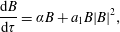 $$\begin{eqnarray}\displaystyle \frac{\text{d}B}{\text{d}\unicode[STIX]{x1D70F}}=\unicode[STIX]{x1D6FC}B+a_{1}B|B|^{2}, & & \displaystyle\end{eqnarray}$$
where
 $$\begin{eqnarray}\displaystyle a_{1}=\frac{1}{Re}\int _{-1}^{1}({\mathcal{G}}_{x}u^{\ast }+{\mathcal{G}}_{y}v^{\ast }+{\mathcal{G}}_{z}w^{\ast }+{\mathcal{G}}\unicode[STIX]{x1D703}^{\ast })\,\text{d}x, & & \displaystyle\end{eqnarray}$$
and is known as the Landau constant, which is the first correction to the linear growth rate. The Landau equation (4.15) represents a modification to the exponential growth or decay of a disturbance predicted by linear theory.
In bifurcation theory, a field within mathematics, a pitchfork bifurcation is a particular type of local bifurcation where the system moves from one fixed point to three fixed points. This is closely tied to the concept of equilibrium amplitude (i.e. the finite amplitude equilibrium solution) and the real part of the Landau coefficient, as shown below.
On substituting
 $A=c_{i}^{1/2}B$
and
 $\unicode[STIX]{x1D70F}=c_{i}t$
into the Landau equation (4.15), the form of the modified Landau equation becomes
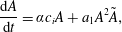 $$\begin{eqnarray}\displaystyle \frac{\text{d}A}{\text{d}t}=\unicode[STIX]{x1D6FC}c_{i}A+a_{1}A^{2}\tilde{A}, & & \displaystyle\end{eqnarray}$$
and its corresponding complex conjugate equation is
 $$\begin{eqnarray}\displaystyle \frac{\text{d}\tilde{A}}{\text{d}t}=\unicode[STIX]{x1D6FC}c_{i}\tilde{A}+\tilde{a_{1}}\tilde{A}^{2}A, & & \displaystyle\end{eqnarray}$$
where
 $\unicode[STIX]{x1D6FC}c_{i}$
is the growth rate from the linear stability analysis and
 $A$
is the physical amplitude of the wave. If we multiply (4.17) by
 $\tilde{A}$
, equation (4.18) by
 $A$
and add, we obtain
 $$\begin{eqnarray}\displaystyle \frac{\text{d}|A|^{2}}{\text{d}t}=2\unicode[STIX]{x1D6FC}c_{i}|A|^{2}+2(a_{1})_{r}|A|^{4}, & & \displaystyle\end{eqnarray}$$
where
 $(a_{1})_{r}$
is the real part of
 $a_{1}$
. The solution,
 $|A|$
, of (4.19) is said to be an equilibrium amplitude (
 $A_{e}$
) provided it satisfies the stationary condition
 $$\begin{eqnarray}\displaystyle {\displaystyle \frac{\text{d}|A|}{\text{d}t}}=0. & & \displaystyle\end{eqnarray}$$
Accordingly, there are three possible equilibrium amplitudes which are given by
 $$\begin{eqnarray}\displaystyle A_{e}=0\quad \text{and}\quad A_{e}=\pm \sqrt{-\unicode[STIX]{x1D6FC}c_{i}/(a_{1})_{r}}. & & \displaystyle\end{eqnarray}$$
Note that
 $A_{e}=0$
, which corresponds to steady basic flow, is stable for
 $Ra<Ra$
(critical) and unstable for
 $Ra>Ra$
(critical). As has been discussed in Drazin & Reid (Reference Drazin and Reid2004) and Shukla & Alam (Reference Shukla and Alam2011), when
 $\unicode[STIX]{x1D6FC}c_{i}$
and
 $(a_{1})_{r}$
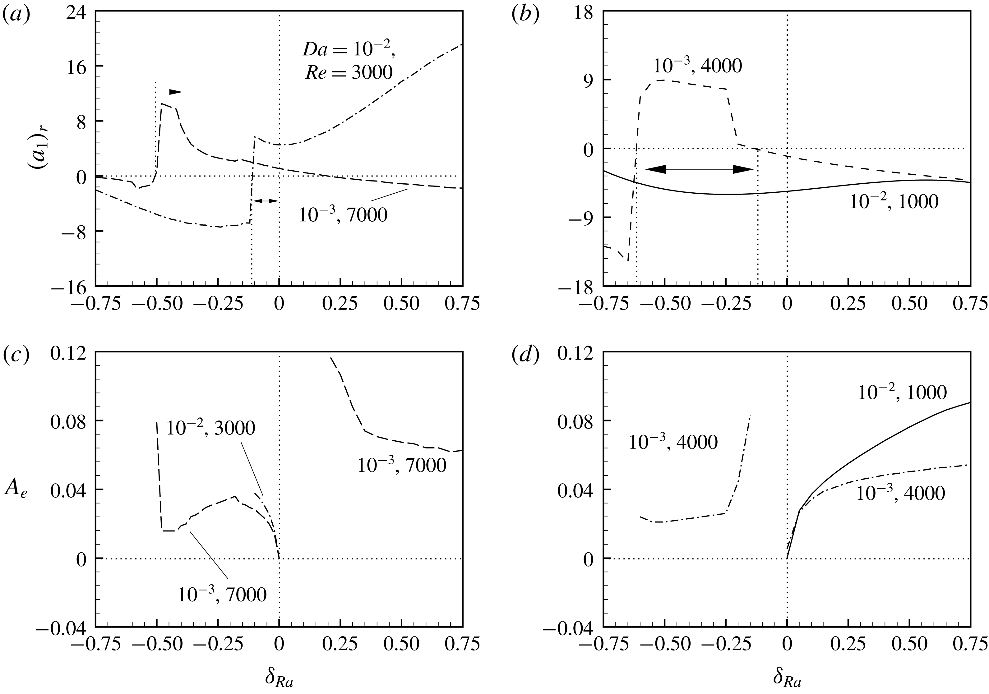
are of the opposite sign, the existence of a finite amplitude solution is guaranteed. Thus, there are two such possible situations: first, the growth rate is positive and the real part of the Landau constant is negative; second, the growth rate is negative and the real part of the Landau constant is positive. The first situation leads to a supercritical pitchfork bifurcation (hereafter, supercritical bifurcation), whereas the second one leads to a subcritical pitchfork bifurcation (hereafter, subcritical bifurcation). For positive growth rates, the nonlinear stationary solution of (4.19) is called the equilibrium amplitude. However, for negative growth rates the nonlinear stationary solution is referred to as the threshold amplitude, since the latter finite amplitude solution is in fact unstable.
4.2 Nonlinear kinetic energy spectrum
To gain further insight into the mechanism of supercritical/subcritical bifurcation, an investigation of the energy transfer in parallel mixed convective flow is made. The Reynolds stress has a significant impact on the basic flow in a weakly nonlinear stability analysis. This distortion of the basic flow modifies the rate of transfer of energy from the basic flow to the disturbance. The balance of kinetic energy for the fundamental disturbance (here onward KE) is given as (Rogers, Moulic & Yao Reference Rogers, Moulic and Yao1993; Khandelwal & Bera Reference Khandelwal and Bera2015)
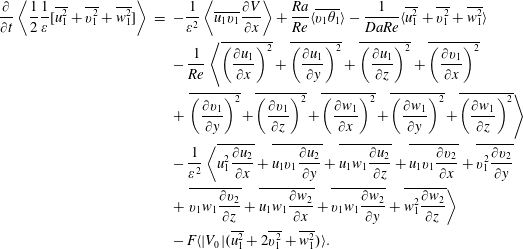 $$\begin{eqnarray}\displaystyle \frac{\unicode[STIX]{x2202}}{\unicode[STIX]{x2202}t}\left\langle \frac{1}{2}\frac{1}{\unicode[STIX]{x1D700}}[\overline{u_{1}^{2}}+\overline{v_{1}^{2}}+\overline{w_{1}^{2}}]\right\rangle & = & \displaystyle -\frac{1}{\unicode[STIX]{x1D700}^{2}}\left\langle \overline{u_{1}v_{1}}\frac{\unicode[STIX]{x2202}V}{\unicode[STIX]{x2202}x}\right\rangle +\frac{Ra}{Re}\langle \overline{v_{1}\unicode[STIX]{x1D703}_{1}}\rangle -\frac{1}{DaRe}\langle \overline{u_{1}^{2}}+\overline{v_{1}^{2}}+\overline{w_{1}^{2}}\rangle \nonumber\\ \displaystyle & & \displaystyle -\,\frac{1}{Re}\left\langle \overline{\left(\frac{\unicode[STIX]{x2202}u_{1}}{\unicode[STIX]{x2202}x}\right)^{2}}+\overline{\left(\frac{\unicode[STIX]{x2202}u_{1}}{\unicode[STIX]{x2202}y}\right)^{2}}+\overline{\left(\frac{\unicode[STIX]{x2202}u_{1}}{\unicode[STIX]{x2202}z}\right)^{2}}+\overline{\left(\frac{\unicode[STIX]{x2202}v_{1}}{\unicode[STIX]{x2202}x}\right)^{2}}\right.\nonumber\\ \displaystyle & & \displaystyle +\left.\overline{\left(\frac{\unicode[STIX]{x2202}v_{1}}{\unicode[STIX]{x2202}y}\right)^{2}}+\overline{\left(\frac{\unicode[STIX]{x2202}v_{1}}{\unicode[STIX]{x2202}z}\right)^{2}}+\overline{\left(\frac{\unicode[STIX]{x2202}w_{1}}{\unicode[STIX]{x2202}x}\right)^{2}}+\overline{\left(\frac{\unicode[STIX]{x2202}w_{1}}{\unicode[STIX]{x2202}y}\right)^{2}}+\overline{\left(\frac{\unicode[STIX]{x2202}w_{1}}{\unicode[STIX]{x2202}z}\right)^{2}}\right\rangle \nonumber\\ \displaystyle & & \displaystyle -\,\frac{1}{\unicode[STIX]{x1D700}^{2}}\left\langle \overline{u_{1}^{2}\frac{\unicode[STIX]{x2202}u_{2}}{\unicode[STIX]{x2202}x}}+\overline{u_{1}v_{1}\frac{\unicode[STIX]{x2202}u_{2}}{\unicode[STIX]{x2202}y}}+\overline{u_{1}w_{1}\frac{\unicode[STIX]{x2202}u_{2}}{\unicode[STIX]{x2202}z}}+\overline{u_{1}v_{1}\frac{\unicode[STIX]{x2202}v_{2}}{\unicode[STIX]{x2202}x}}+\overline{v_{1}^{2}\frac{\unicode[STIX]{x2202}v_{2}}{\unicode[STIX]{x2202}y}}\right.\nonumber\\ \displaystyle & & \displaystyle +\left.\overline{v_{1}w_{1}\frac{\unicode[STIX]{x2202}v_{2}}{\unicode[STIX]{x2202}z}}+\overline{u_{1}w_{1}\frac{\unicode[STIX]{x2202}w_{2}}{\unicode[STIX]{x2202}x}}+\overline{v_{1}w_{1}\frac{\unicode[STIX]{x2202}w_{2}}{\unicode[STIX]{x2202}y}}+\overline{w_{1}^{2}\frac{\unicode[STIX]{x2202}w_{2}}{\unicode[STIX]{x2202}z}}\right\rangle \nonumber\\ \displaystyle & & \displaystyle -\,F\langle |V_{0}|(\overline{u_{1}^{2}}+2\overline{v_{1}^{2}}+\overline{w_{1}^{2}})\rangle .\end{eqnarray}$$
Here, the bracket
 $\langle ~\rangle$
implies integration over the volume of the disturbance wave and
 $\overline{GH}$
for some field variables
 $G$
and
 $H$
is defined as
 $G\tilde{H}+\tilde{G}H$
. With the help of (4.15), the balance of kinetic energy leads to an amplitude equation (Rogers et al.
Reference Rogers, Moulic and Yao1993)
 $$\begin{eqnarray}\displaystyle \frac{\text{d}|B|^{2}}{\text{d}\unicode[STIX]{x1D70F}}=2\unicode[STIX]{x1D6FC}|B|^{2}+(P_{101}+E_{12}+P_{110}+T_{11}+D_{11}+K_{11}+F_{11})|B|^{4}. & & \displaystyle\end{eqnarray}$$
The comparison of (4.15) and (4.23) shows that
 $$\begin{eqnarray}\displaystyle 2(a_{1})_{r}=P_{101}+E_{12}+P_{110}+T_{11}+D_{11}+K_{11}+F_{11}, & & \displaystyle\end{eqnarray}$$
where the right-hand side quantities are defined as
 $$\begin{eqnarray}\displaystyle P_{101}=-\frac{1}{e_{0}\unicode[STIX]{x1D700}^{2}}\left\langle \overline{u_{10}v_{10}}\frac{\text{d}V_{1}}{\text{d}x}\right\rangle , & & \displaystyle\end{eqnarray}$$
 $$\begin{eqnarray}\displaystyle E_{12} & = & \displaystyle -\frac{1}{e_{0}\unicode[STIX]{x1D700}^{2}}\left\langle \overline{u_{10}^{2}\frac{\unicode[STIX]{x2202}u_{20}}{\unicode[STIX]{x2202}x}}+\overline{u_{10}v_{10}\frac{\unicode[STIX]{x2202}u_{20}}{\unicode[STIX]{x2202}y}}+\overline{u_{10}w_{10}\frac{\unicode[STIX]{x2202}u_{20}}{\unicode[STIX]{x2202}z}}\right.\nonumber\\ \displaystyle & & \displaystyle +\,\overline{u_{10}v_{10}\frac{\unicode[STIX]{x2202}v_{20}}{\unicode[STIX]{x2202}x}}+\overline{v_{10}^{2}\frac{\unicode[STIX]{x2202}v_{20}}{\unicode[STIX]{x2202}y}}+\overline{v_{10}w_{10}\frac{\unicode[STIX]{x2202}v_{20}}{\unicode[STIX]{x2202}z}}\nonumber\\ \displaystyle & & \displaystyle +\left.\overline{u_{10}w_{10}\frac{\unicode[STIX]{x2202}w_{20}}{\unicode[STIX]{x2202}x}}+\overline{v_{10}w_{10}\frac{\unicode[STIX]{x2202}w_{20}}{\unicode[STIX]{x2202}y}}+\overline{w_{10}^{2}\frac{\unicode[STIX]{x2202}w_{20}}{\unicode[STIX]{x2202}z}}\right\rangle ,\end{eqnarray}$$
 $$\begin{eqnarray}\displaystyle & \displaystyle P_{110}=-\frac{1}{e_{0}\unicode[STIX]{x1D700}^{2}}\left\langle (\overline{u_{10}v_{11}}+\overline{v_{10}u_{11}})\frac{\text{d}V_{0}}{\text{d}x}\right\rangle , & \displaystyle\end{eqnarray}$$
 $$\begin{eqnarray}\displaystyle & \displaystyle T_{11}=\frac{1}{e_{0}}\frac{Ra}{Re}\langle \overline{v_{10}\unicode[STIX]{x1D703}_{11}}+\overline{\unicode[STIX]{x1D703}_{10}v_{11}}\rangle , & \displaystyle\end{eqnarray}$$
 $$\begin{eqnarray}\displaystyle D_{11} & = & \displaystyle -\frac{1}{e_{0}}\frac{1}{Re}\left\langle \overline{\frac{\unicode[STIX]{x2202}u_{10}}{\unicode[STIX]{x2202}x}\frac{\unicode[STIX]{x2202}u_{11}}{\unicode[STIX]{x2202}x}}+\overline{\frac{\unicode[STIX]{x2202}u_{10}}{\unicode[STIX]{x2202}y}\frac{\unicode[STIX]{x2202}u_{11}}{\unicode[STIX]{x2202}y}}+\overline{\frac{\unicode[STIX]{x2202}u_{10}}{\unicode[STIX]{x2202}z}\frac{\unicode[STIX]{x2202}u_{11}}{\unicode[STIX]{x2202}z}}\right.\nonumber\\ \displaystyle & & \displaystyle +\,\overline{\frac{\unicode[STIX]{x2202}v_{10}}{\unicode[STIX]{x2202}x}\frac{\unicode[STIX]{x2202}v_{11}}{\unicode[STIX]{x2202}x}}+\overline{\frac{\unicode[STIX]{x2202}v_{10}}{\unicode[STIX]{x2202}y}\frac{\unicode[STIX]{x2202}v_{11}}{\unicode[STIX]{x2202}y}}+\overline{\frac{\unicode[STIX]{x2202}v_{10}}{\unicode[STIX]{x2202}z}\frac{\unicode[STIX]{x2202}v_{11}}{\unicode[STIX]{x2202}z}}\nonumber\\ \displaystyle & & \displaystyle +\left.\overline{\frac{\unicode[STIX]{x2202}w_{10}}{\unicode[STIX]{x2202}x}\frac{\unicode[STIX]{x2202}w_{11}}{\unicode[STIX]{x2202}x}}+\overline{\frac{\unicode[STIX]{x2202}w_{10}}{\unicode[STIX]{x2202}y}\frac{\unicode[STIX]{x2202}w_{11}}{\unicode[STIX]{x2202}y}}+\overline{\frac{\unicode[STIX]{x2202}w_{10}}{\unicode[STIX]{x2202}z}\frac{\unicode[STIX]{x2202}w_{11}}{\unicode[STIX]{x2202}z}}\right\rangle ,\end{eqnarray}$$
 $$\begin{eqnarray}\displaystyle & \displaystyle K_{11}=-\frac{2}{e_{0}DaRe}\langle \overline{u_{10}u_{11}}+\overline{v_{10}v_{11}}+\overline{w_{10}w_{11}}\rangle , & \displaystyle\end{eqnarray}$$
 $$\begin{eqnarray}\displaystyle & \displaystyle F_{11}=-\frac{2}{e_{0}}F\langle |V_{0}|(\overline{u_{10}u_{11}}+2\overline{v_{10}v_{11}}+\overline{w_{10}w_{11}})\rangle , & \displaystyle\end{eqnarray}$$
and
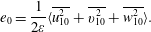 $$\begin{eqnarray}\displaystyle e_{0}=\frac{1}{2\unicode[STIX]{x1D700}}\langle \overline{u_{10}^{2}}+\overline{v_{10}^{2}}+\overline{w_{10}^{2}}\rangle . & & \displaystyle\end{eqnarray}$$
The physical interpretation of different terms in the balance of KE, given in (4.24), is as follows. The term
 $P_{101}$
, which is an integral of the product of the Reynolds stress and the mean velocity gradient, denotes the gradient production of KE due to the interaction between the fundamental mode (quantities assigned subscript 10) and the distorted mean flow strain rate. The energy needed for the distortion of the mean flow is obtained from the fundamental disturbance, consequently, this term will be negative. Hence, this term will reduce the growth rate of the disturbance. The second term
 $E_{12}$
represents the transfer of the KE from the fundamental to the second harmonic wave (quantities assigned subscript 20). The other five terms
 $P_{110}$
,
 $T_{11}$
,
 $D_{11}$
,
 $K_{11}$
and
 $F_{11}$
account for the energy exchange due to the modification of the shape of the fundamental disturbance wave. The term
 $P_{110}$
arises because of the modification to the gradient production of KE, and may have a positive or negative sign. The positive sign of
 $P_{110}$
indicates that the change in the shape of the fundamental disturbance will be more favourable for shear production. The term
 $T_{11}$
represents the modification to the buoyant production of KE. The terms
 $D_{11}$
,
 $K_{11}$
and
 $F_{11}$
represent dissipation of KE through modification to the viscous dissipation rate, modification to the surface drag and modification to the form drag, respectively.
5 Numerical procedure
In the present work a spectral Chebyshev collocation method is employed to find the solution of the basic state, linear stability and nonlinear stability equations. The equations are discretized along the
 $x$
-direction by implementing the spectral collocation method that uses Chebyshev polynomials as the basis functions. The governing equations are collocated at Gauss–Lobatto points. The Gauss–Lobatto points of an
 $N$
th-order Chebyshev polynomial are given as
 $$\begin{eqnarray}\displaystyle x_{j}=\cos \left(\frac{\unicode[STIX]{x03C0}j}{N}\right), & & \displaystyle\end{eqnarray}$$
where
 $j=0,1,2,\ldots ,N$
and
 $N$
represents the order of the base polynomial. The details of the spectral collocation technique can be found in the book by Canuto et al. (Reference Canuto, Hussaini, Quarteroni and Zang1986). The discretized linear disturbance equations (C 1)–(C 5) along with the homogeneous boundary conditions (3.7) are formulated as a generalized eigenvalue problem given by (3.8). The square complex matrices
 $\unicode[STIX]{x1D63C}$
and
 $\unicode[STIX]{x1D63D}$
are of order
 $3N+3$
(after elimination of the pressure term). The eigenvalues of the generalized eigenvalue problem (3.8) are calculated by the QZ-algorithm of the MATLAB software using the eig command. The adjoint eigenfunctions are used in the integrability condition to determine the first Landau coefficient. The set of adjoint equations of the linear stability problem are also solved by the same spectral method. For nonlinear stability analysis, we need to solve the related non-homogeneous differential equations in
 $\mathscr{A}X=b$
form, where
 $\mathscr{A}=\unicode[STIX]{x1D63C}-c\unicode[STIX]{x1D63D}$
. In the case of the
 $E^{2}$
harmonic component, the system
 $\mathscr{A}=\unicode[STIX]{x1D63C}-c\unicode[STIX]{x1D63D}$
is non-singular as
 $\unicode[STIX]{x1D6FC}$
and
 $\unicode[STIX]{x1D6FD}$
in (4.10)–(4.14) are replaced by
 $2\unicode[STIX]{x1D6FC}$
and
 $2\unicode[STIX]{x1D6FD}$
respectively, and the complex wave speed
 $(c)$
of the fundamental wave
 $(E^{1})$
is not an eigenvalue of this system. So, the eigenvalues are not identical and there is no theoretical difficulty in solving the equations of the
 $E^{2}$
harmonic component. For the calculation of
 $u_{11},v_{11},w_{11},p_{11}$
and
 $\unicode[STIX]{x1D703}_{11}$
, we encounter a singular system of equations of the form
 $\mathscr{A}X_{1}=b$
, which is solved by the singular value decomposition (SVD) method which is built into the MATLAB software. These sets of equations are also discretized by the same spectral collocation method and the integrals occurring everywhere are calculated by the Gauss–Chebyshev quadrature integration formula.
The numerical code developed in the earlier work (Khandelwal & Bera Reference Khandelwal and Bera2015) for the stability of the non-isothermal Poiseuille flow in a fluid-filled vertical channel is extended for the present problem. The accuracy and validity of the numerical scheme are checked by comparing our general results with published results (Chen & Chung Reference Chen and Chung1996; Khandelwal & Bera Reference Khandelwal and Bera2015), by taking
 $Da=10^{12}$
,
 $F^{\prime }=0$
and
 $\unicode[STIX]{x1D700}=1$
. The solution generated by the code is in excellent agreement with the published results. Apart from this, the results remain consistent when the order of the polynomial
 $(N)$
is 50 or more (table not shown), which was determined after many preliminary tests. Therefore, all of the computations are reported by taking the order of the polynomial as 50.
6 Results and discussion
To give an illustration, we carry out a finite amplitude instability analysis of a stably stratified PMCF in a vertical channel filled with a fluid-saturated porous medium. The linear stability results show that a two-dimensional disturbance with
 $\unicode[STIX]{x1D6FD}=0$
is the most unstable wave for a stably stratified flow. As a consequence, the present nonlinear stability results are carried out for
 $\unicode[STIX]{x1D6FD}=0$
. The cubic Landau equation (4.15) derived in terms of the amplitude function is used to identify the supercritical/subcritical bifurcation. In the following, we discuss the impact of nonlinear interaction of the different harmonics on the type of bifurcation, equilibrium amplitude, physical quantities (i.e. heat transfer rate and skin friction coefficient), kinetic energy spectrum, as well as pattern of secondary flow. This has been carried out in the neighbourhood of the bifurcation point as well as away from the bifurcation point. For this a new parameter,
 $\unicode[STIX]{x1D6FF}_{Ra}$
, defined by
 $\unicode[STIX]{x1D6FF}_{Ra}=Ra/Ra_{c}-1$
is introduced.
6.1 Landau constant in the neighbourhood of the bifurcation point
The Landau constant is calculated at
 $\unicode[STIX]{x1D6FF}_{Ra}=\pm 0.01$
(i.e. in the vicinity of the critical Rayleigh number) with respect to the most unstable linear wave (with critical wavenumber
 $(\unicode[STIX]{x1D6FC}_{c})$
). Note that
 $\unicode[STIX]{x1D6FF}_{Ra}=-0.01(+0.01)$
is a point from a linearly stable (unstable) region, and the corresponding growth rate is negative (positive). To identify the nature of the bifurcation of the flow, the real part of the Landau constant (
 $(a_{1})_{r}$
) as a function of
 $Re$
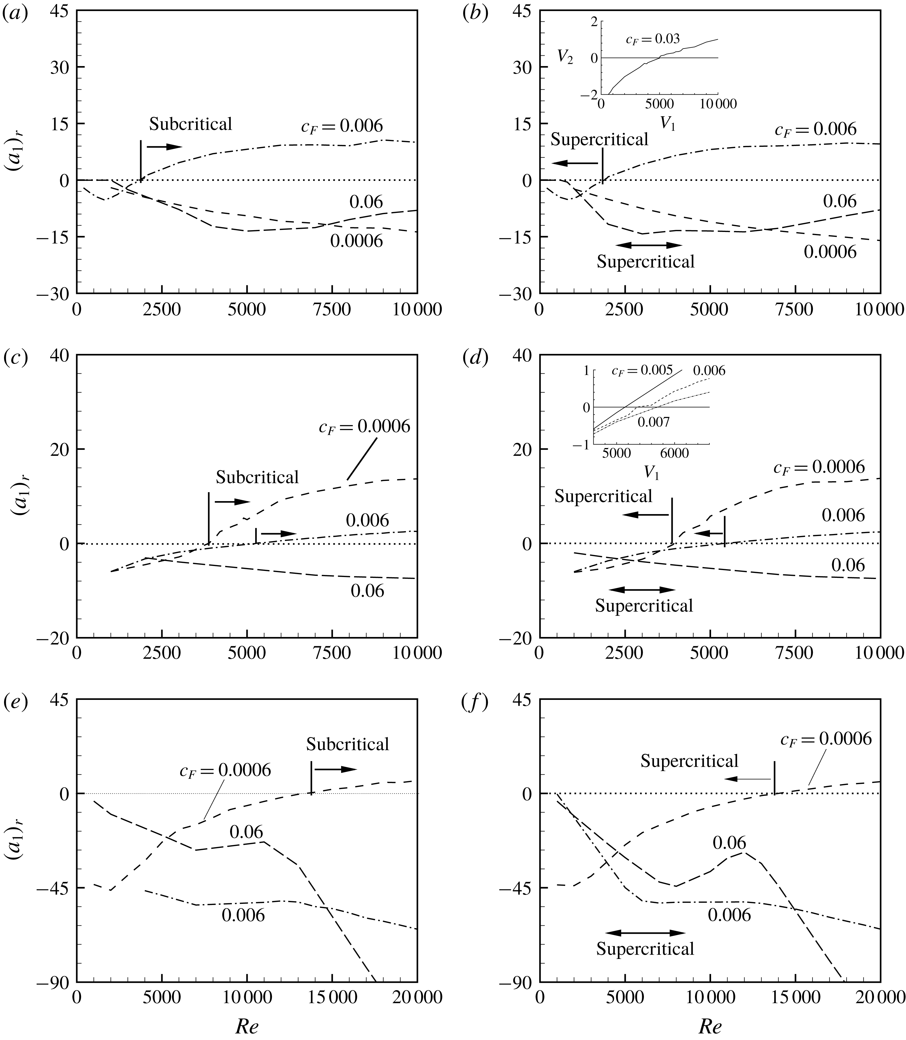
is plotted. The variation of
 $(a_{1})_{r}$
at
 $\unicode[STIX]{x1D6FF}_{Ra}=-0.01(+0.01)$
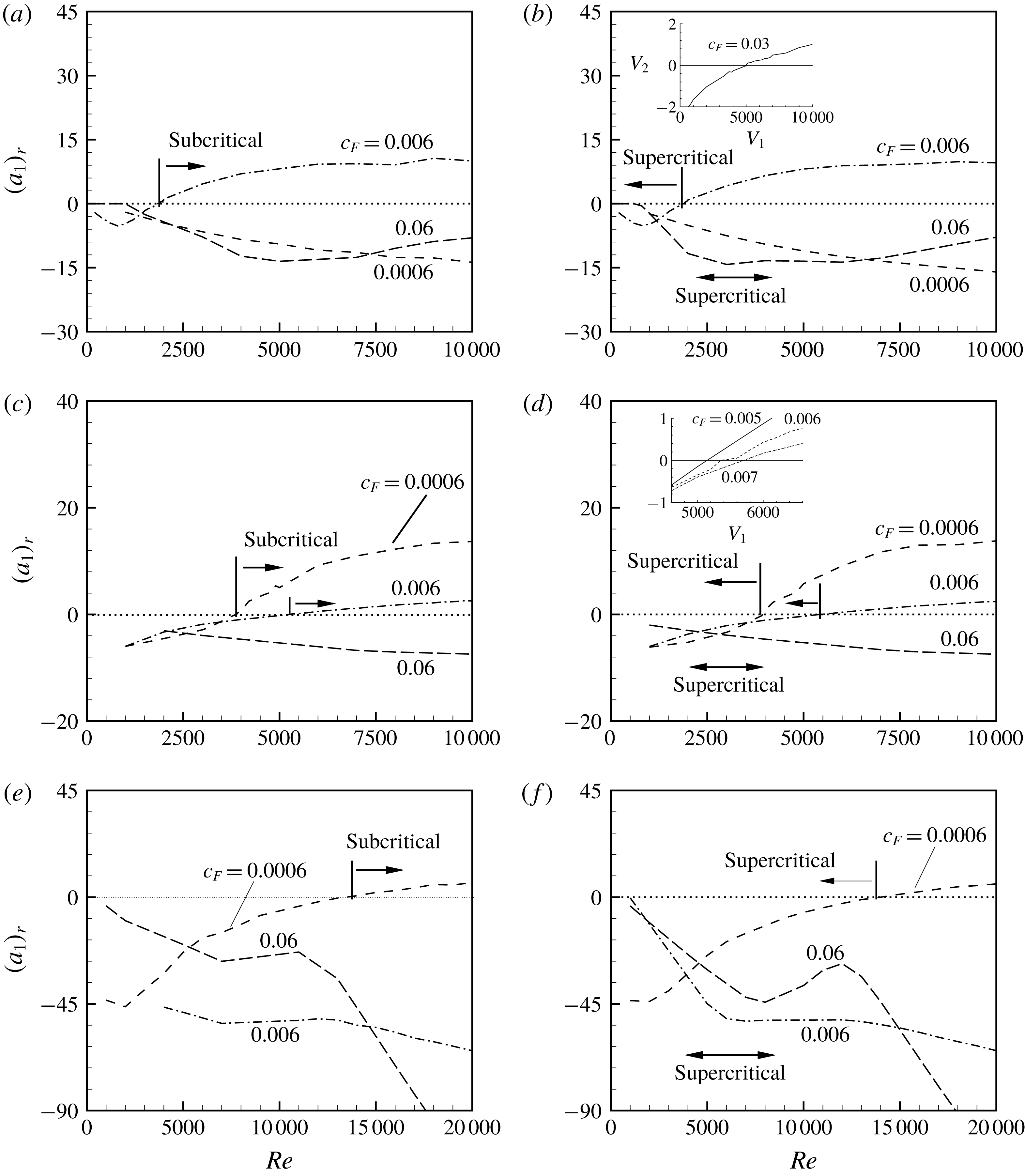
, when the porous medium is saturated by air, is shown in figures 4(a,b), 4(c,d) and 4(e,f) for
 $Da$
equal to
 $10^{-2}$
,
 $10^{-3}$
and
 $10^{-4}$
, respectively. As can be seen from figure 4(a,b), the sign of
 $(a_{1})_{r}$
is negative for
 $Da=10^{-2}$
with
 $c_{F}=0.0006$
as well as 0.06, indicating the supercritical bifurcation (see figure 4
b). However, on replacing the value 0.0006 of
 $c_{F}$
by 0.006 the same figures show supercritical bifurcation for
 $Re<1900$
and subcritical bifurcation for
 $Re>1900$
. Let
 $Re_{sb}$
denote the minimum value of
 $Re$
at which the shifting of bifurcation from supercritical to subcritical takes place. Accordingly, in this case, the value of
 $Re_{sb}$
is 1900. Note that the value of
 $(a_{1})_{r}$
is zero at
 $Re=Re_{sb}$
. In general, the value of
 $Re_{sb}$
increases on increasing the value of
 $c_{F}$
. For example, when the value 0.006 of
 $c_{F}$
is replaced by 0.03, the value of
 $Re_{sb}$
becomes 5000 (see figure 4
b). Furthermore, for each value of
 $c_{F}$
, figures 4(c) and 4(d) as well as the inset therein, show, in general, the existence of a
 $Re_{sb}$
. The values of
 $Re_{sb}$
for
 $c_{F}$
equal to 0.0006 and 0.006 are 4000 and 5340, respectively. For
 $Da=10^{-4}$
, figure 4(e,f) shows mainly a supercritical bifurcation except for
 $c_{F}=0.0006$
where the shifting of the bifurcation also takes place at
 $Re_{sb}=14\,000$
. Interestingly,
 $Re_{sb}$
increases on increasing the value of
 $c_{F}$
as well as on decreasing the value of
 $Da$
. This may be a consequence of the following fact. Since a decrease in the permeability of the medium or an increase in the form drag, in general, stabilizes the flow, therefore to achieve a change of bifurcation in PMCF in a porous medium in which the permeability is relatively low or induced form drag is relatively high, a relatively higher disturbance shear production is required.
Variation of Landau constant (
 $(a_{1})_{r}$
) with respect to
 $Re$
: (a,b)
 $Da=10^{-2}$
, (c,d)
 $Da=10^{-3}$
and (e,f)
 $Da=10^{-4}$
when
 $Pr=0.7$
; (a,c,e)
 $\unicode[STIX]{x1D6FF}_{Ra}=-0.01$
, and (b,d,f)
 $\unicode[STIX]{x1D6FF}_{Ra}=0.01$
.
Variation of threshold amplitude in the subcritical region (solid line) as well as equilibrium amplitude in the supercritical region with respect to
 $Re$
: (a)
 $Da=10^{-2}$
, (b)
 $Da=10^{-3}$
and (c)
 $Da=10^{-4}$
when
 $Pr=0.7$
.
The corresponding threshold amplitude in the subcritical region as well as the equilibrium amplitude in the supercritical region for
 $Da$
equal to
 $10^{-2}$
,
 $10^{-3}$
and
 $10^{-4}$
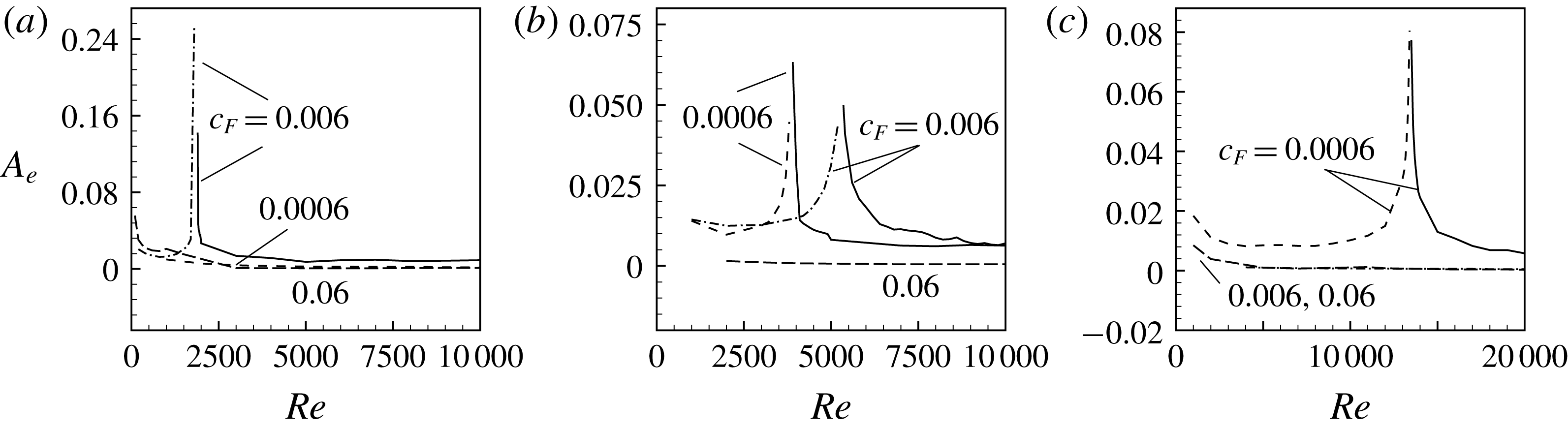
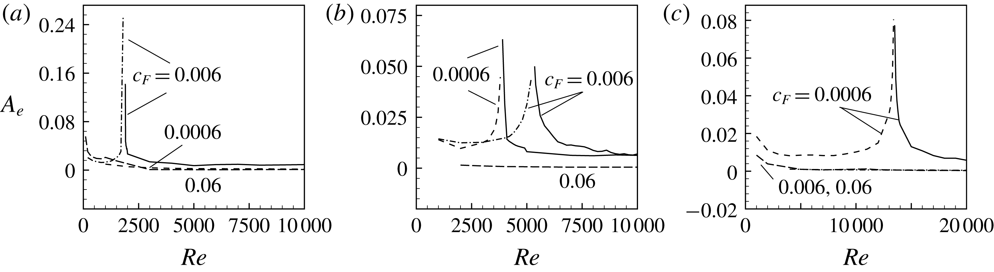
, are displayed in figures 5(a), 5(b) and 5(c), respectively. The solid line in each graph denotes the amplitude profile in the subcritical region. It is important to mention here that for
 $\unicode[STIX]{x1D6FF}_{Ra}=0.01$
(i.e. positive growth rate) if the sign of
 $(a_{1})_{r}$
is positive then
 $A_{e}$
does not exist. Similarly, for
 $\unicode[STIX]{x1D6FF}_{Ra}=-0.01$
if the sign of
 $(a_{1})_{r}$
is negative then
 $A_{e}$
does not exist. Consequently, the amplitude in the above figure is drawn in the subcritical (i.e.
 $\unicode[STIX]{x1D6FF}_{Ra}=-0.01$
) as well as in supercritical (i.e.
 $\unicode[STIX]{x1D6FF}_{Ra}=0.01$
) regimes only. Each of the above figures manifests an important feature. The notable feature is the sudden jump in the amplitude profile in the vicinity of
 $Re_{sb}$
, where the supercritical bifurcation changes to a subcritical one or vice versa. Note that at
 $Re_{sb}$
the function
 $A_{e}$
is not defined and the variation of growth rate in the vicinity of
 $Re_{sb}$
is almost constant (see figure 19
a,b in appendix B.2). Therefore, the above-mentioned sudden jump of the amplitude in the vicinity of
 $Re_{sb}$
may be a consequence of the very small value of
 $(a_{1})_{r}$
, and
 $A_{e}$
being inversely proportional to the square root of
 $(a_{1})_{r}$
. The jump in the amplitude profile is expected to lead to complex phenomena in the flow instability. More about its impact on the instability mechanism will be discussed later in this section.
To show the variation of
 $(a_{1})_{r}$
and the equilibrium amplitude as a function of
 $Re$
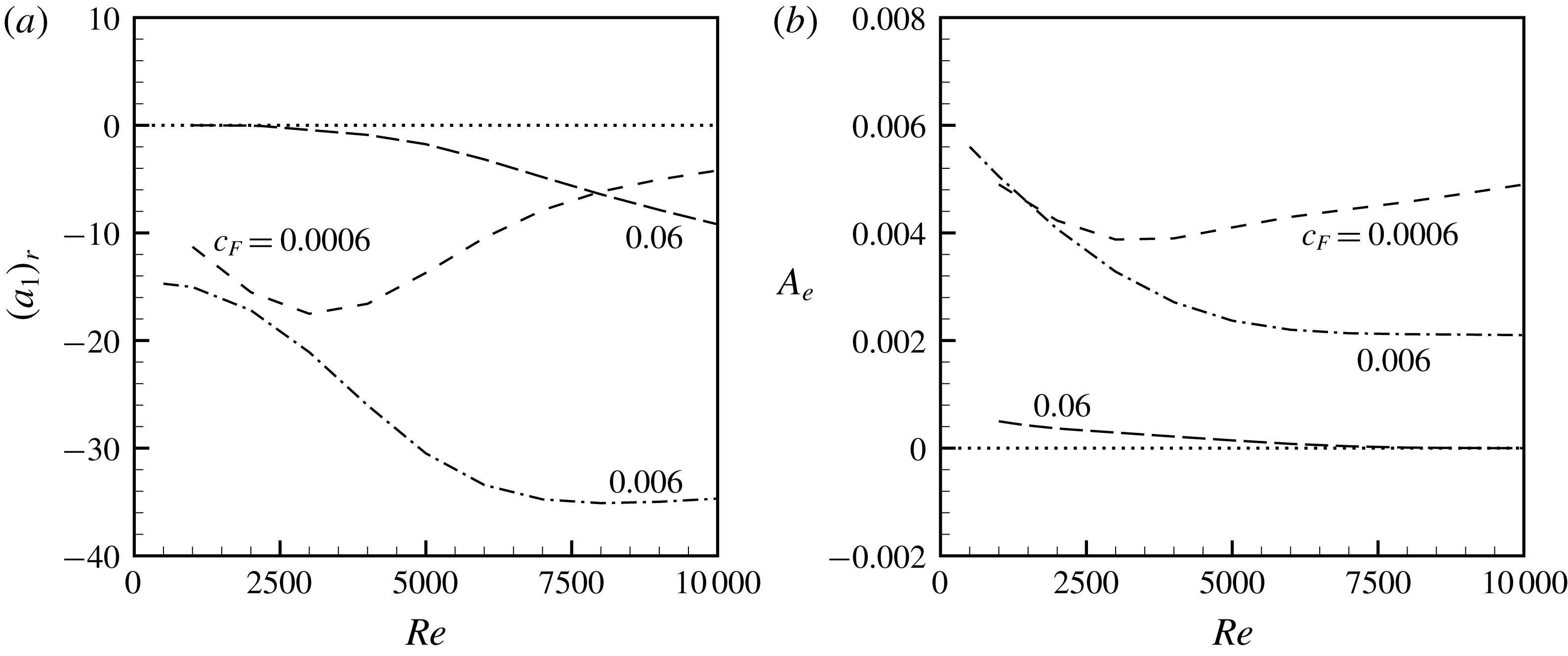
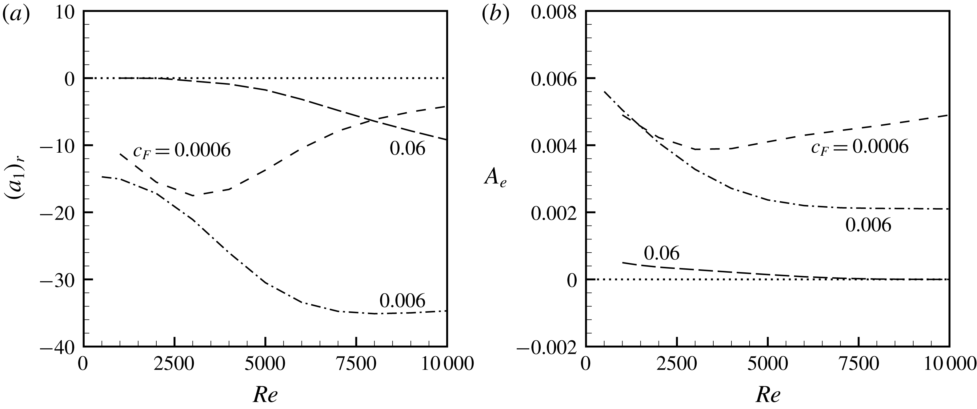
, when the porous medium is saturated by water, respectively figures 6(a) and 6(b) are drawn for
 $Da$
equal to
 $10^{-3}$
in the linearly unstable regime at
 $\unicode[STIX]{x1D6FF}_{Ra}=0.01$
. As can be seen from figure 6(a), the sign of
 $(a_{1})_{r}$
is negative, for all considered values of
 $c_{F}$
, i.e. only supercritical bifurcations exist. The corresponding amplitude profiles shown in figure 6(b) vary smoothly. Note that the calculated values of
 $(a_{1})_{r}$
for both values (0.01 and
 $-$
0.01) of
 $\unicode[STIX]{x1D6FF}_{Ra}$
are almost identical for air, which is also true for water. Therefore, variation of
 $(a_{1})_{r}$
at
 $\unicode[STIX]{x1D6FF}_{Ra}=-0.01$
is not shown here. Apart from this, it has been also checked that in a water-saturated porous medium the sign of
 $(a_{1})_{r}$
is negative for all other considered values of
 $Da$
. So, the variation of
 $(a_{1})_{r}$
for all other values of
 $Da$
is also not shown here. Since we are interested in the situation where a change of bifurcation takes place, therefore, in the rest of this subsection we shall be restricted to only an air-saturated porous medium.
Variation of Landau constant (a) and equilibrium amplitude (b) with respect to
 $Re$
when
 $Da=10^{-3}$
and
 $Pr=7$
.
The above observations make us curious to know about the variation of physical quantities such as the heat transfer rate in terms of the Nusselt number and the friction coefficient as a function of
 $Re$
, especially in the neighbourhood of the point where a change of bifurcation takes place. As we have seen, in general
 $c_{F}$
delays the shifting whereas
 $Da$
accelerates it. Therefore, in the rest of the analysis in this subsection, we have fixed the value of
 $Da$
at
 $10^{-3}$
,
 $c_{F}$
at 0.006 and
 $Pr$
at 0.7.
6.1.1 Nusselt number and friction coefficient as a function of
 $Re$

The heat transfer rate in terms of the Nusselt number is defined as
 $$\begin{eqnarray}\displaystyle Nu=-2H_{1}/H_{2}, & & \displaystyle\end{eqnarray}$$
where
 $H_{1}$
and
 $H_{2}$
are given by
 $\unicode[STIX]{x2202}\unicode[STIX]{x1D6E9}/\unicode[STIX]{x2202}x|_{x=1}$
and
 $\int _{-1}^{1}V\unicode[STIX]{x1D6E9}\,\text{d}x/\int _{-1}^{1}V\text{d}x$
, respectively. The functions
 $V$
and
 $\unicode[STIX]{x1D6E9}$
, calculated using the threshold or equilibrium amplitude, are given as
 $V_{0}+{A_{e}}^{2}V_{1}$
and
 $\unicode[STIX]{x1D6E9}_{0}+{A_{e}}^{2}\unicode[STIX]{x1D6E9}_{1}$
, respectively. The functions
 $V_{1}$
and
 $\unicode[STIX]{x1D6E9}_{1}$
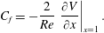
are the basic flow distortion functions. Similarly, the friction coefficient at the wall is given as (Schlichting & Gersten Reference Schlichting and Gersten2004)
 $$\begin{eqnarray}\displaystyle C_{f}=-\frac{2}{Re}\left.\frac{\unicode[STIX]{x2202}V}{\unicode[STIX]{x2202}x}\right|_{x=1}. & & \displaystyle\end{eqnarray}$$
The friction coefficient at the other wall of the channel (
 $x=-1$
) is also the same as the wall
 $x=1$
.
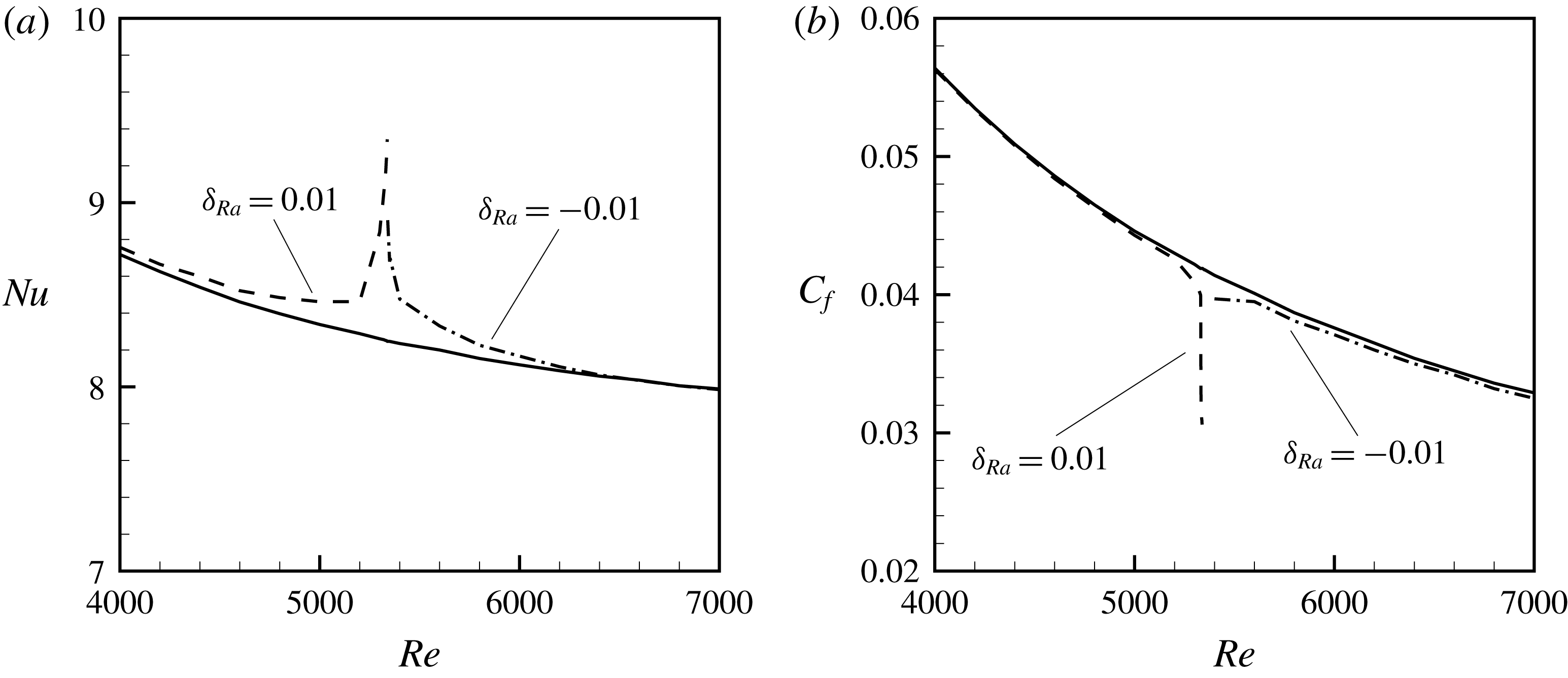
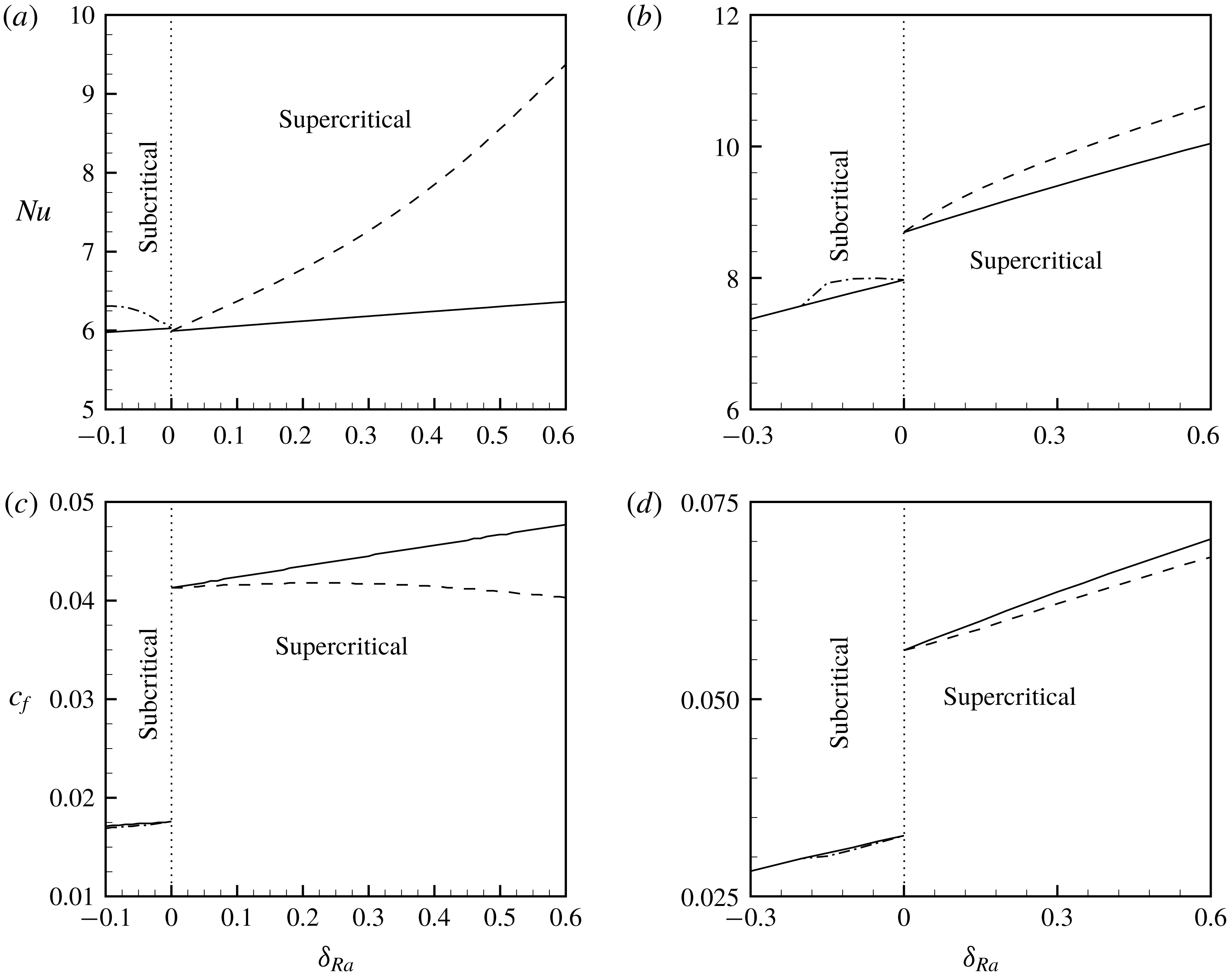
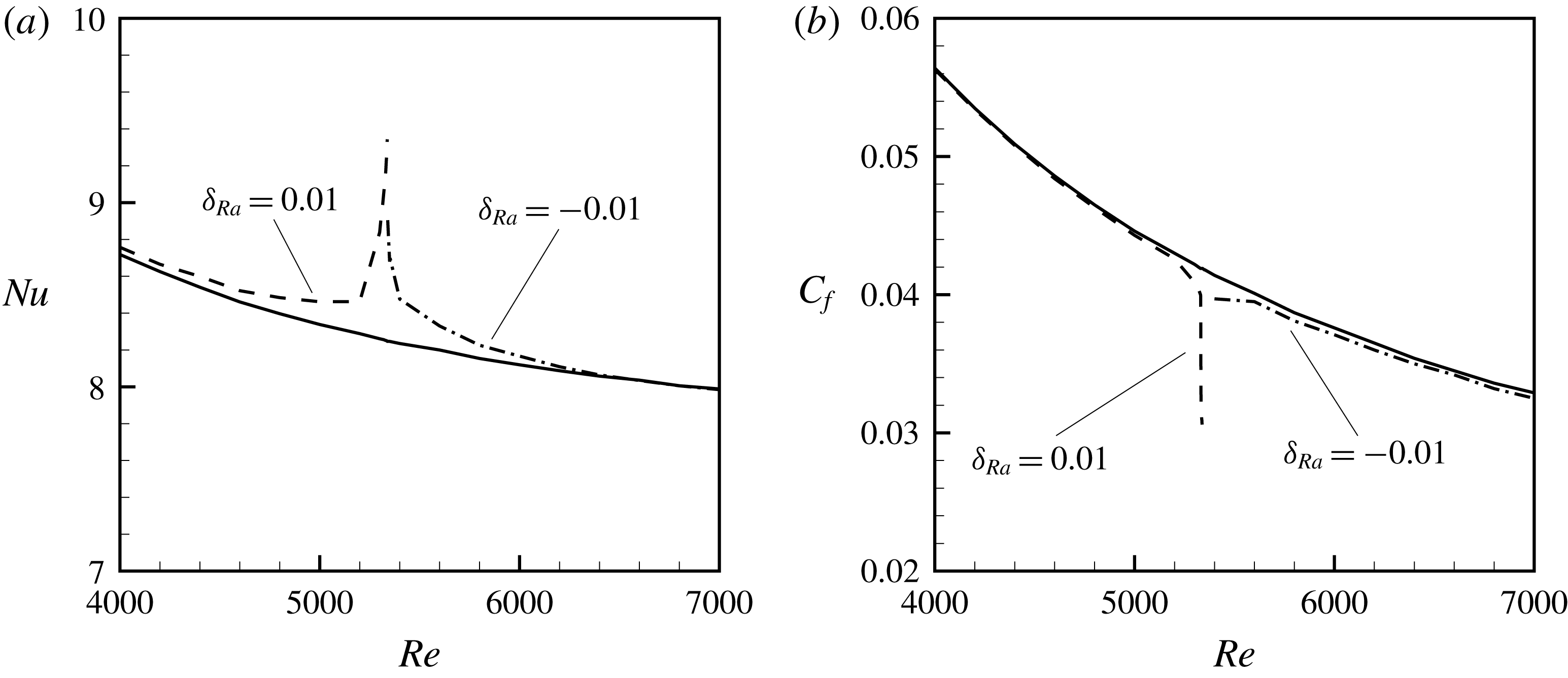
The impact of disturbance growth/decay on the heat transfer rate in the region of subcritical as well as supercritical bifurcation is examined in figure 7(a). The dash-dotted line is curved in the subcritical region. Let
 $Nu_{bs}$
and
 $Nu_{ds}$
be defined as the Nusselt numbers predicted for the basic state (solid line) and the distorted state (dashed line as well as dash-dotted line), respectively (see figure 7
a), then the results show that the Nusselt number estimated with the help of weakly nonlinear stability analysis is more or less the same as the one calculated for the basic state, except in the vicinity where the type of bifurcation changes. In this vicinity,
 $Nu_{ds}$
is not defined at
 $Re=Re_{sb}$
. The impact of nonlinear interaction between different harmonic modes on the friction coefficient is displayed in figure 7(b). Similar to
 $Nu_{ds}$
, the difference between the friction coefficient for the distorted state (
 $C_{fds}$
) and basic state (
 $C_{fbs}$
) is also negligible, but the magnitude of
 $C_{fds}$
decreases significantly in the vicinity where the change in bifurcation takes place. The distorted friction coefficient is also not defined at
 $Re=Re_{sb}$
. It should be noted that the above phenomenon (rapid change of
 $Nu_{ds}$
as well as
 $C_{fds}$
in the vicinity of
 $Re_{sb}$
) was also reported for purely fluid medium (Suslov & Paolucci Reference Suslov and Paolucci1999b
) while studying nonlinear stability of a mixed convection flow under a non-Boussinesq condition in a differentially heated channel.
Variation of Nusselt number and friction coefficient with respect to
 $Re$
when
 $Da=10^{-3}$
,
 $Pr=0.7$
and
 $c_{F}=6\times 10^{-3}$
. The solid line represents the basic state, whereas the dash-dotted and dashed lines represent the distorted state.
6.1.2 Nonlinear energy spectrum as a function of
$Re$

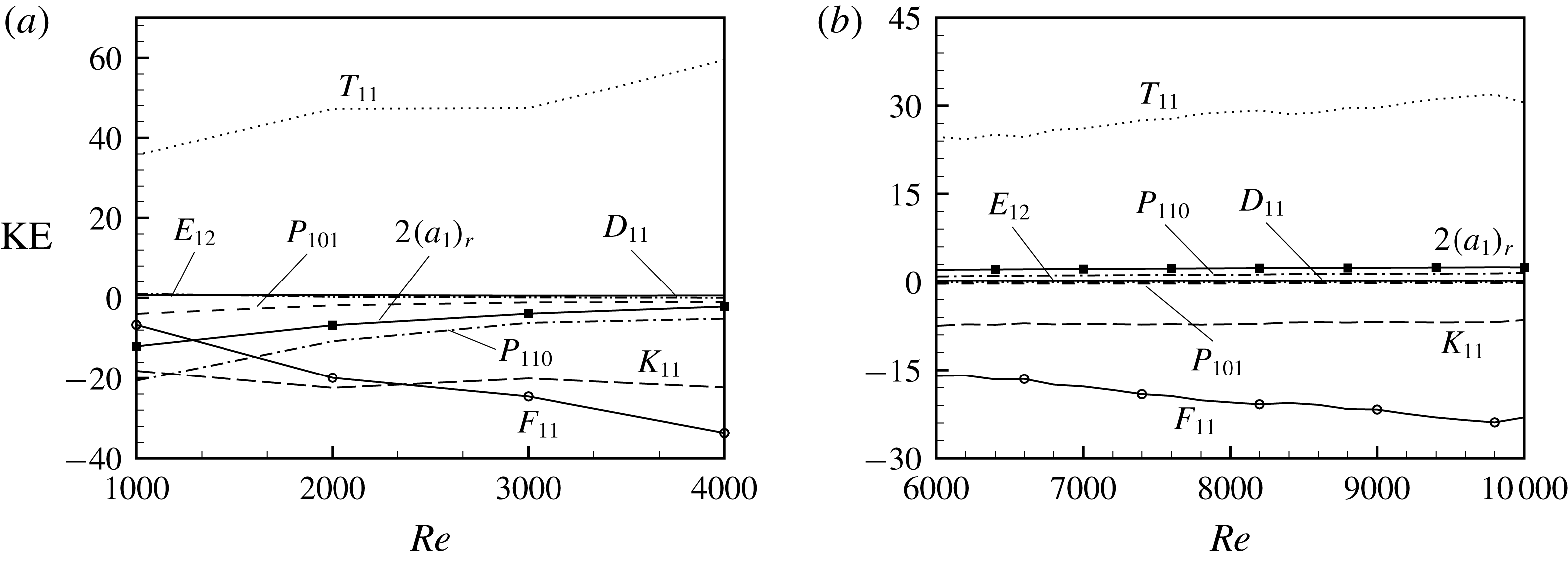
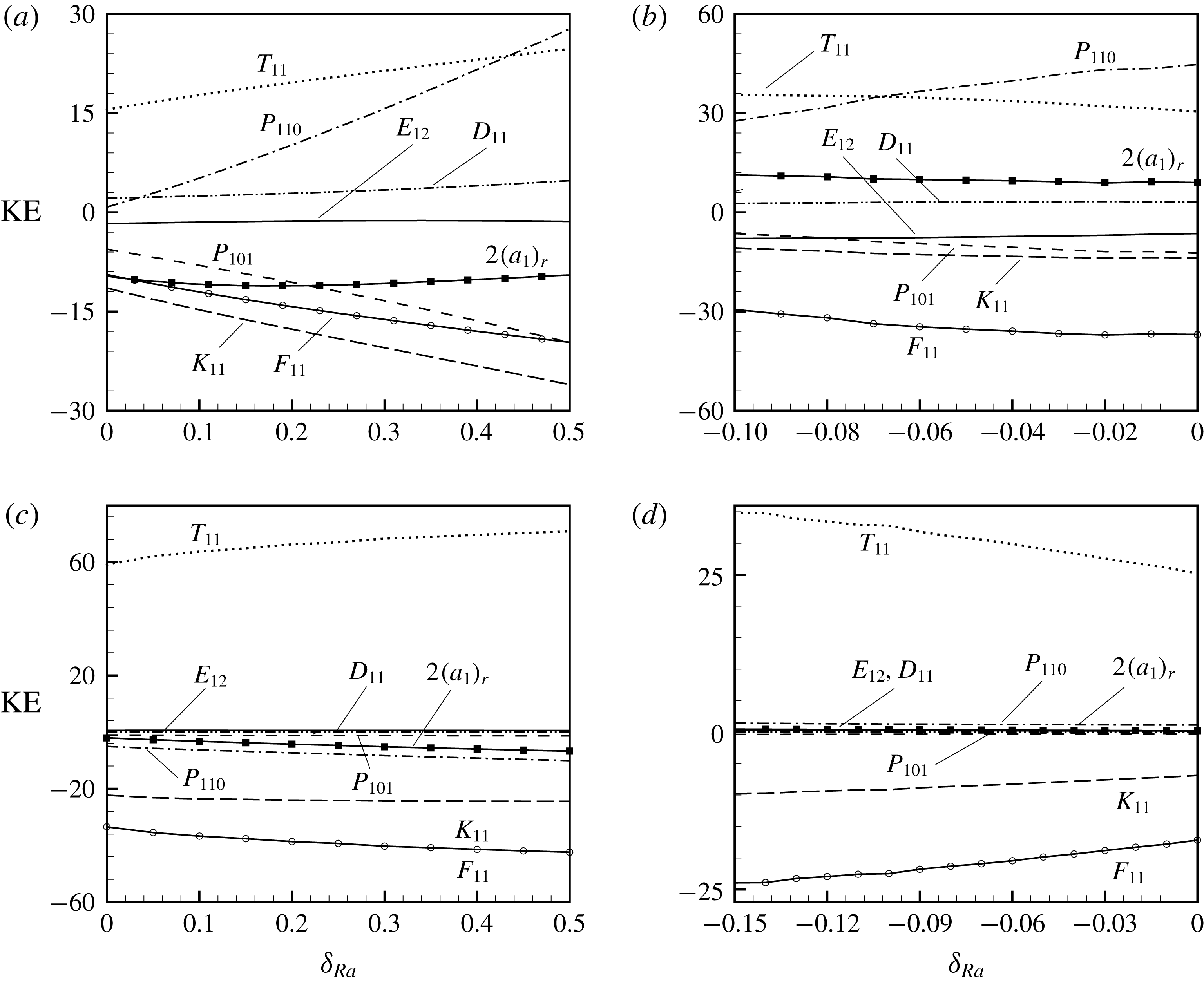
To understand the driving mechanisms of flow instability and change of bifurcation at a neighbouring point of the least linearly stable point, the spectrum of nonlinear kinetic energy balance of the fundamental disturbance (KE) in the supercritical regime (at
 $\unicode[STIX]{x1D6FF}_{Ra}=0.01$
) and the subcritical regime (at
 $\unicode[STIX]{x1D6FF}_{Ra}=-0.01$
) is shown in figures 8(a) and 8(b), respectively. Note that the mathematical analysis of the nonlinear kinetic energy spectrum shows that the sum of the different energy terms is twice the real part of the Landau constant (see (4.24)). Therefore, the type of bifurcation predicted by the Landau constant can be reconfirmed through the sum of the different energy terms. Consequently, the sum is also shown in both figures 8(a) and 8(b). The following points can be noted from figure 8(a,b). The term
 $P_{101}$
is negative in both (super- and subcritical) regimes which implies that the gradient production of the KE for supercritical flow always tends to stabilize. Its magnitude decreases on increasing
 $Re$
and the contribution to the energy spectrum becomes almost negligible. The magnitude of the term
 $E_{12}$
or
 $D_{11}$
is very small, i.e. the transfer of KE from fundamental to the harmonic waves or modification to the dissipation of KE due to a change in the disturbance shape is also negligible. In both regimes, the modified disturbance shape is favourable to buoyant production of the KE (i.e.
 $T_{11}$
is positive throughout the range of
 $Re$
) and acts as the main destabilizing factor. In the subcritical regime,
 $T_{11}$
is balanced mainly by dissipation of KE through induced surface drag (
 $K_{11}$
) and form drag (
 $F_{11}$
). However, in the supercritical regime, apart from
 $K_{11}$
,
 $F_{11}$
, another term
 $P_{110}$
also takes a significant role in the KE balance, especially for relatively low values of
 $Re$
. In the supercritical regime, the term
 $P_{110}$
is negative and its magnitude decreases on increasing
 $Re$
, i.e. the stabilizing impact decreases on increasing
 $Re$
, whereas in the subcritical regime it is positive and its contribution to the energy spectrum is almost negligible. A negative sign of
 $P_{110}$
indicates that the change in the shape of the fundamental disturbance is not favourable to shear production. It is important to mention here that for the present parametric set values of
 $Da$
and
 $c_{F}$
the contribution of the shear term,
 $E_{s}$
, in linear theory is negative and the type of instability is buoyant (see discussion § 3.1); therefore, the dominance of
 $T_{11}$
in both regimes is a consequence of the buoyant instability of the flow. We are also curious to know whether any relation between the sign of
 $E_{s}$
in linear theory and the sign of
 $P_{110}$
in weakly nonlinear analysis exists or not. This issue will be discussed further in § 6.2. Finally, figure 8(a,b) shows the negative (positive) value of the sum of all the terms (i.e.
 $(2a_{1})_{r}$
) of the KE spectrum. So, the analysis of the nonlinear kinetic energy spectrum also predicts the supercritical (subcritical) bifurcation in figure 8(a,b).
Variation of KE with respect to
 $Re$
for
 $Da=10^{-3}$
,
 $Pr=0.7$
and
 $c_{F}=6\times 10^{-3}$
: (a) supercritical regime (
 $\unicode[STIX]{x1D6FF}_{Ra}=0.01$
) of
 $Re$
, (b) subcritical regime (
 $\unicode[STIX]{x1D6FF}_{Ra}=-0.01$
) of
 $Re$
.
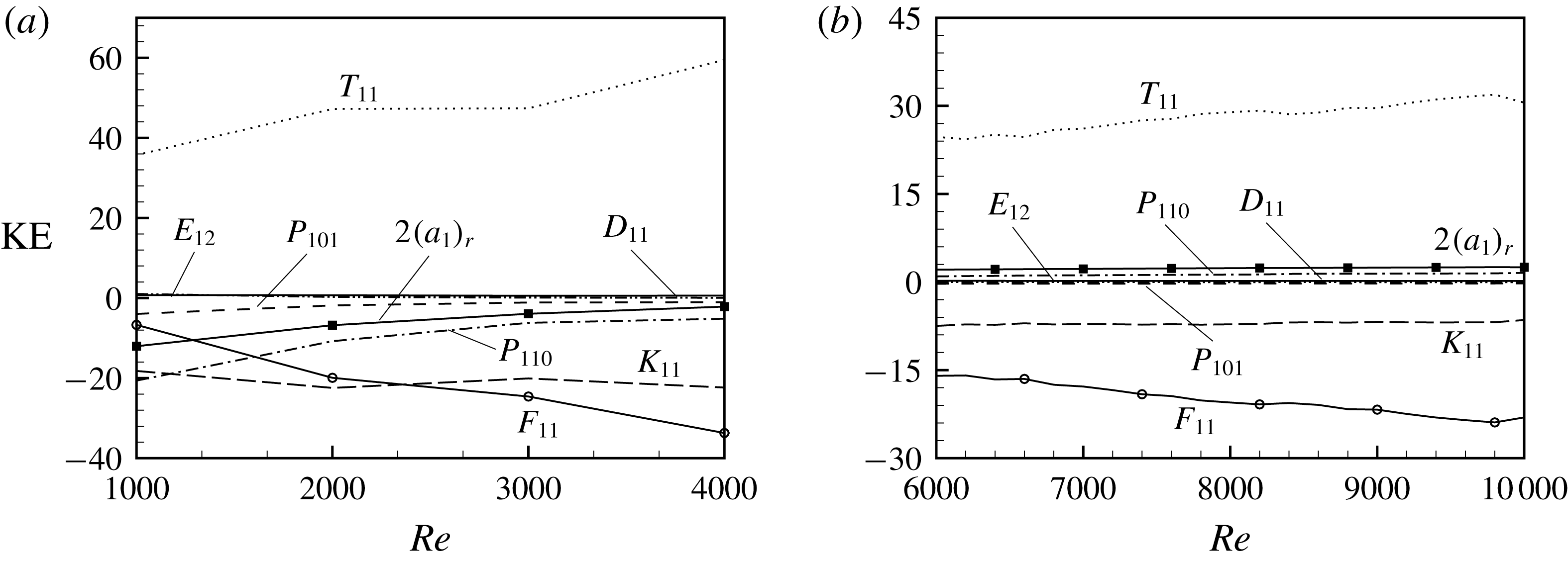
6.2 Bifurcation as a function of
$Ra$

Weakly nonlinear analysis is only valid near the linear stability boundary point (Drazin & Reid Reference Drazin and Reid2004) and it addresses the question of what happens to an unstable flow. Rogers et al. (Reference Rogers, Moulic and Yao1993) have shown, by comparison with the results from the direct numerical simulation as well as high-order weakly nonlinear results, that the cubic Landau equation gives the correct results when the magnitude of
 $c_{i}$
is small. They have also pointed out that the weakly nonlinear analysis is asymptotically correct for larger values of the Rayleigh number beyond the bifurcation point in the limit of
 $c_{i}$
approaching zero. Based on this fact, for a given
 $Re$
, we have studied the behaviour of the Landau constant as well as the equilibrium amplitude away from the critical
 $Ra$
(i.e. in the linearly stable and unstable regimes), as a function of
 $\unicode[STIX]{x1D6FF}_{Ra}$
. For this we have chosen four pairs of (
 $Da$
,
 $Re$
), two each from the supercritical and subcritical regimes. Here,
 $c_{F}$
is fixed at 0.006. Accordingly, for two values
 $10^{-2}$
and
 $10^{-3}$
of
 $Da$
, two different respective values, 1000 and 4000, of
 $Re$
from the supercritical regime and two respective values, 3000 and 7000, of
 $Re$
from the subcritical regime are chosen. The corresponding critical values of
 $Ra$
are 290, 12 269, 425, 12 366, respectively. We have checked from our numerical experiments by calculating the growth rate as a function of
 $\unicode[STIX]{x1D6FF}_{Ra}$
that the magnitude of
 $c_{i}$
for all of the above values of
 $Re$
is of the order of
 $10^{-2}$
in the considered range of
 $\unicode[STIX]{x1D6FF}_{Ra}$
(see figure 20 in appendix B.2). Therefore, we also analyse the limiting value of growth of the instabilities under nonlinear effects (i.e. nonlinear saturation) for larger (lower) values of the Rayleigh number beyond (before) the bifurcation point. However, a complete picture of nonlinear saturation can only be confirmed by use of direct numerical simulation, which is beyond the scope of the present work. Hence, the following analysis will give a qualitative characteristic of the nonlinear interaction of different harmonic modes for larger (lower) values of
 $Ra$
beyond (before) the bifurcation point.
Variation of
 $(a_{1})_{r}$
and amplitude with respect to
 $\unicode[STIX]{x1D6FF}_{Ra}$
when
 $Pr=0.7$
and
 $c_{F}=6\times 10^{-3}$
: (a,c) subcritical regime of
 $Re$
, (b,d) supercritical regime of
 $Re$
.
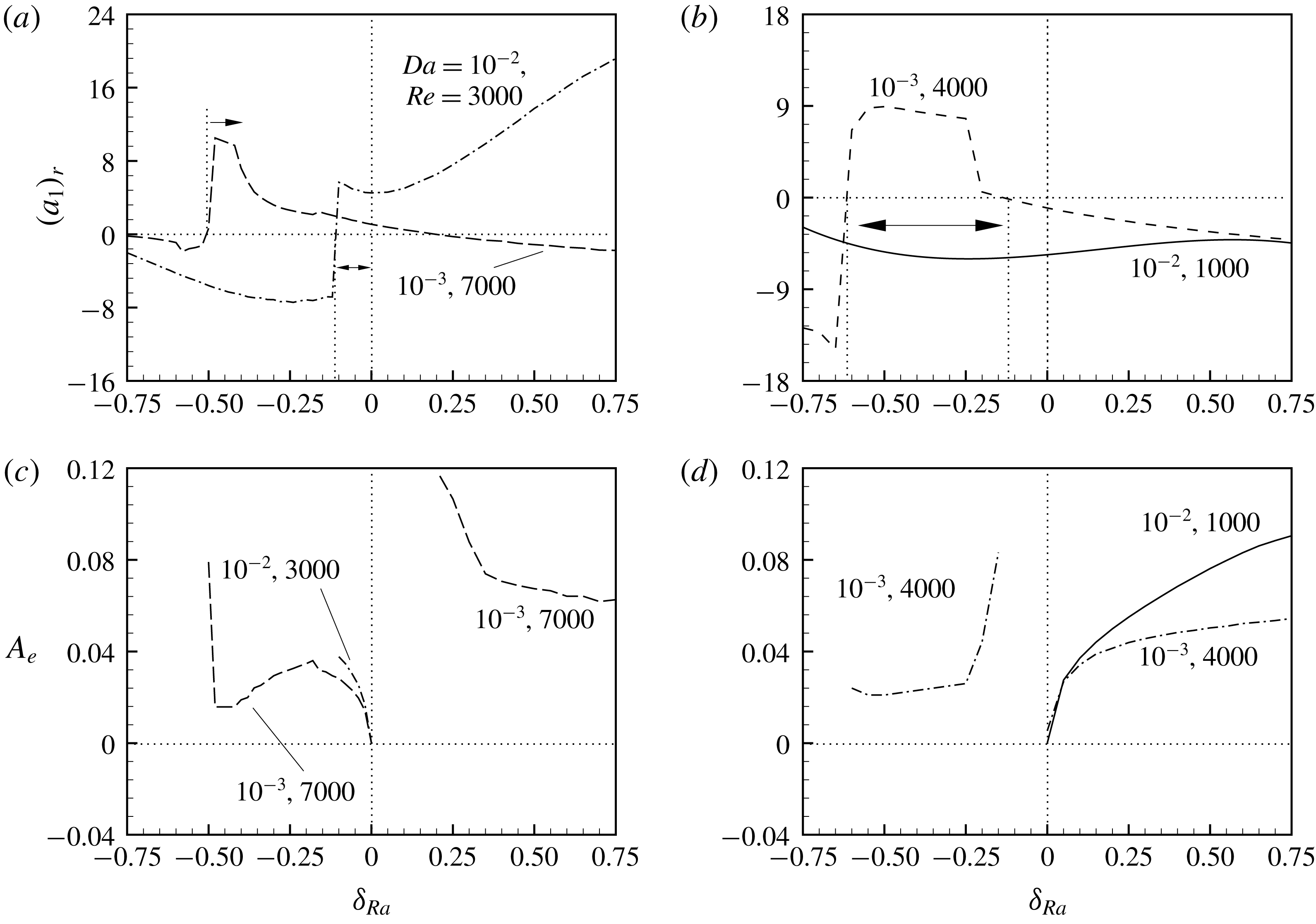
The variation of the real part of the Landau constant, for pairs of (
 $Da$
,
 $Re$
) chosen from the subcritical and supercritical regimes, as a function of
 $\unicode[STIX]{x1D6FF}_{Ra}$
is shown in figures 9(a) and 9(b), respectively. As can be seen from figure 9(a), when
 $Da=10^{-3}$
,
 $Re=7000$
and the corresponding critical value of
 $Ra$
is 12 366, the sign of
 $(a_{1})_{r}$
in the linearly stable regime (i.e.
 $\unicode[STIX]{x1D6FF}_{Ra}<0$
) remains positive for
 $\unicode[STIX]{x1D6FF}_{Ra}\geqslant -0.5$
, i.e. for
 $Ra\geqslant 6183$
. This indicates that
 $Ra=6183$
acts as a lower critical value, below which the bifurcated solution does not exist (Drazin & Reid Reference Drazin and Reid2004), and
 $-0.5\leqslant \unicode[STIX]{x1D6FF}_{Ra}\leqslant 0$
is a regime of subcritical bifurcation. Similarly, when
 $Da=10^{-2}$
,
 $Re=3000$
and the corresponding critical value of
 $Ra$
is 425, the sign of
 $(a_{1})_{r}$
in the linearly stable regime remains positive for
 $\unicode[STIX]{x1D6FF}_{Ra}\geqslant -0.1$
, i.e. for
 $Ra\geqslant 382.5$
. So, in this case,
 $Ra=382.5$
acts as a lower critical value, below which the bifurcated solution does not exist. Therefore, we can conclude that
 $6183\leqslant Ra\leqslant 12\,366$
(
 $382.5\leqslant Ra\leqslant 425$
) is a regime of subcritical bifurcation when
 $Da=10^{-3}$
and
 $Re=7000$
(
 $Da=10^{-2}$
and
 $Re=3000$
). In the linearly unstable regime, the same figure also shows the positive sign of
 $(a_{1})_{r}$
when
 $Da=10^{-2}$
,
 $Re=3000$
, However, in the case of
 $Da=10^{-3}$
,
 $Re=7000$
the sign of
 $(a_{1})_{r}$
remains positive up to
 $\unicode[STIX]{x1D6FF}_{Ra}=0.17$
, beyond which it becomes negative. This leads to supercritical bifurcation for
 $\unicode[STIX]{x1D6FF}_{Ra}>0.17$
. So, in this case the subcritical bifurcation changes to supercritical bifurcation. Note that the above-mentioned lower critical values obtained through the cubic Landau equation are only probable values. To get the exact value of
 $Ra$
in the subcritical region where the unstable threshold branch turns and becomes stable, a fifth-order Landau equation is required, which is beyond the scope of the present study.
Furthermore, the positive sign of
 $(a_{1})_{r}$
in the linearly unstable regime (i.e. positive growth rate) implies that both terms on the right-hand side of the Landau equation (4.19) are positive and therefore
 $|A|$
increases exponentially and the solution breaks down after a finite time. Of course this kind of breakdown does not occur in practice; rather, the breakdown points to the need for terms in higher powers of
 $|A|$
(Drazin & Reid Reference Drazin and Reid2004), which is beyond the scope of the present work.
For the other two pairs
 $(10^{-2},1000)$
and
 $(10^{-3},4000)$
of (
 $Da$
,
 $Re$
) chosen from the supercritical regime, figure 9(b) shows that the sign of
 $(a_{1})_{r}$
remains negative in the linearly stable as well as the unstable regime for
 $(Da,Re)=(10^{-2},1000)$
. This implies that the supercritical bifurcation of the flow remains supercritical even when
 $Ra$
is increased to 1.75 times its critical value. However, for
 $(Da,Re)=(10^{-3},4000)$
it is different. In this case, the sign of
 $(a_{1})_{r}$
in the linearly stable regime is positive for
 $-0.6\leqslant \unicode[STIX]{x1D6FF}_{Ra}\leqslant -0.15$
, consequently a regime of subcritical bifurcation appears and gives a lower critical value of
 $Ra=4907.6$
.
The variation of the amplitude as a function of
 $\unicode[STIX]{x1D6FF}_{Ra}$
for (
 $Da$
,
 $Re$
) chosen from the subcritical and supercritical regimes are shown in figures 9(c) and 9(d), respectively. As can be seen from figure 9(c), in the subcritical regime
 $A_{e}$
increases on increasing the magnitude of
 $\unicode[STIX]{x1D6FF}_{Ra}$
for
 $Re=3000$
, but for
 $Re=7000$
the same increases up to
 $\unicode[STIX]{x1D6FF}_{Ra}=-0.17$
and it decreases when
 $-0.17>\unicode[STIX]{x1D6FF}_{Ra}>-0.5$
. The increasing characteristic of
 $A_{e}$
away from the bifurcation point is a consequence of the fact that the magnitude of the growth rate increases (see figure 20 in appendix B.2) and
 $(a_{1})_{r}$
remains almost constant. In the supercritical regime, figure 9(d) shows that
 $A_{e}$
increases on increasing
 $\unicode[STIX]{x1D6FF}_{Ra}$
which is mainly due to increasing characteristic of the growth rate as a function of
 $\unicode[STIX]{x1D6FF}_{Ra}$
.
A similar study is also made when the medium is saturated with water (a figure is not shown here). However, the variation of the Landau constant as a function of
 $Ra$
predicts only the supercritical bifurcation. Therefore, in the rest of the section our analysis will be restricted to the impact of nonlinear interaction on the PMCF of air only.
To understand the impact of nonlinear effects on heat transfer rate and friction coefficient away from the bifurcation point, for the same set of
 $(Da,Ra)$
, figure 10(a,c) is drawn for
 $Da=10^{-2}$
and figure 10(b,d) is drawn for
 $Da=10^{-3}$
. As can be seen from figures 10(a) and 10(b), the Nusselt number estimated in the linearly unstable regime with the help of a weakly nonlinear stability analysis is more than the one calculated from the basic state. The substantial increase in
 $Nu_{ds}$
beyond the bifurcation point can be predicted due to the buoyant instability of the flow. Quantitatively, we have observed that the increase in
 $Nu$
due to nonlinear interaction is around 35 % for
 $(Da,Re)=(10^{-2},1000)$
(5.6 % for
 $(Da,Re)=(10^{-3},4000)$
) at
 $\unicode[STIX]{x1D6FF}_{Ra}=0.5$
. However, for
 $Re$
in the subcritical regime, the change in
 $Nu$
under the basic state and the distorted state can be seen up to
 $\unicode[STIX]{x1D6FF}_{Ra}=-0.1$
(
 $\unicode[STIX]{x1D6FF}_{Ra}=-0.17$
) for
 $Re=3000$
(
 $Re=7000$
). The friction coefficient,
 $C_{f}$
, for the above four values of
 $Re$
is shown in figure 10(c,d). The friction coefficient due to nonlinear interaction in the linearly unstable regime is less compared to the same calculated in the basic state. It decreases as a function of
 $Ra$
. Quantitatively, the decrease in friction coefficient due to nonlinear interaction at
 $\unicode[STIX]{x1D6FF}_{Ra}=0.5$
in the supercritical regime is around 12.42 % for
 $(Da,Re)=(10^{-2},1000)$
(3 % for
 $(Da,Re)=(10^{-3},4000)$
). However, it is almost zero in the linearly stable regime.
Variation of (a,b) Nusselt number and (c,d) friction coefficient with respect to
 $\unicode[STIX]{x1D6FF}_{Ra}$
in the subcritical (
 $Re=3000$
,
 $Re=7000$
) and supercritical regime (
 $Re=1000$
,
 $Re=4000$
) for
 $Pr=0.7$
and
 $c_{F}=6\times 10^{-3}$
. The solid line represents the basic state, whereas the dash-dotted as well as dashed lines represent the distorted state. Here, (a,c)
 $Da=10^{-2}$
, (b,d)
 $Da=10^{-3}$
.
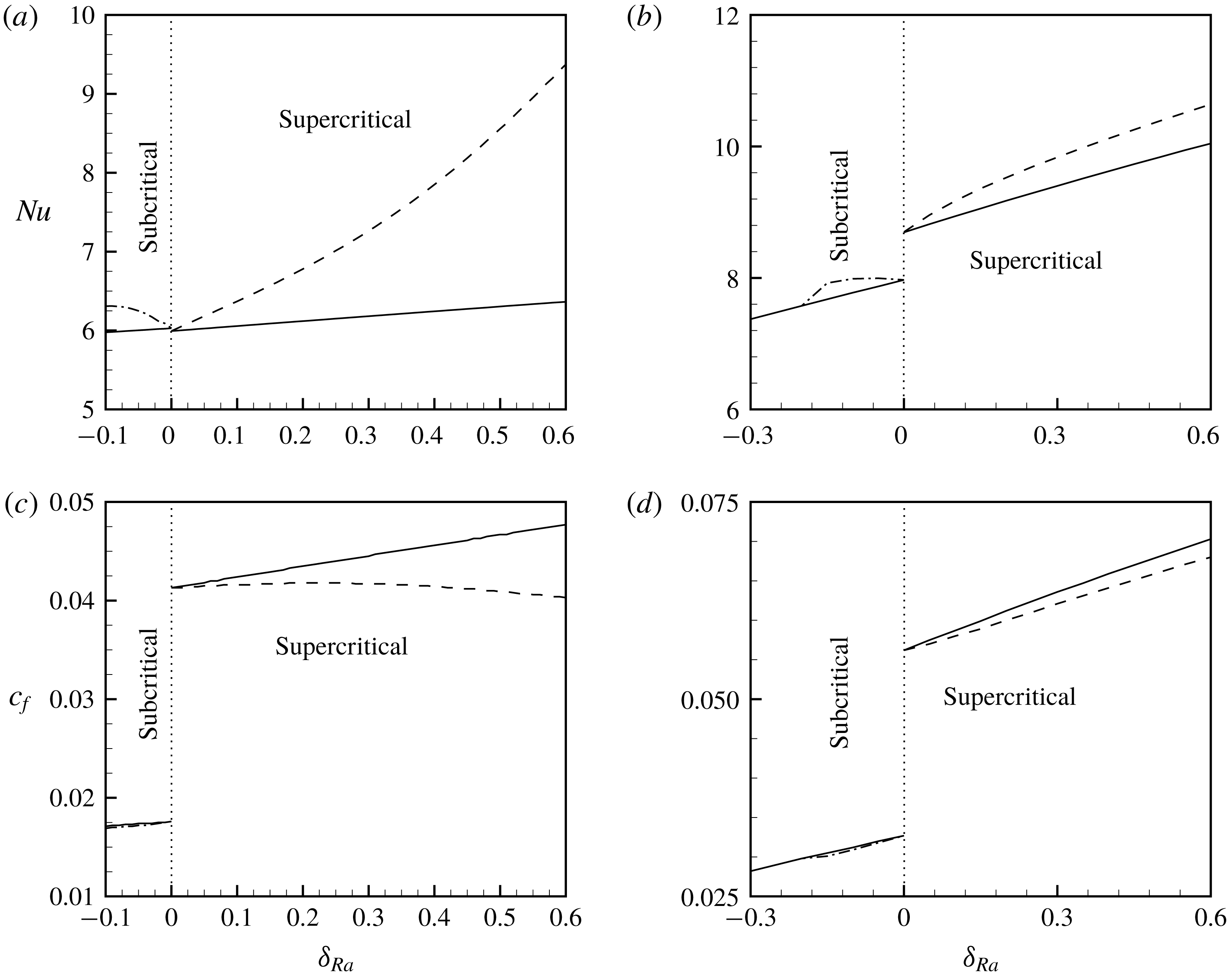
Variation of KE with respect to
 $\unicode[STIX]{x1D6FF}_{Ra}$
for
 $Pr=0.7$
and
 $c_{F}=6\times 10^{-3}$
: (a)
 $Re=1000$
,
 $Da=10^{-2}$
, (b)
 $Re=3000$
,
 $Da=10^{-2}$
, (c)
 $Re=4000$
,
 $Da=10^{-3}$
and (d)
 $Re=7000$
,
 $Da=10^{-3}$
.
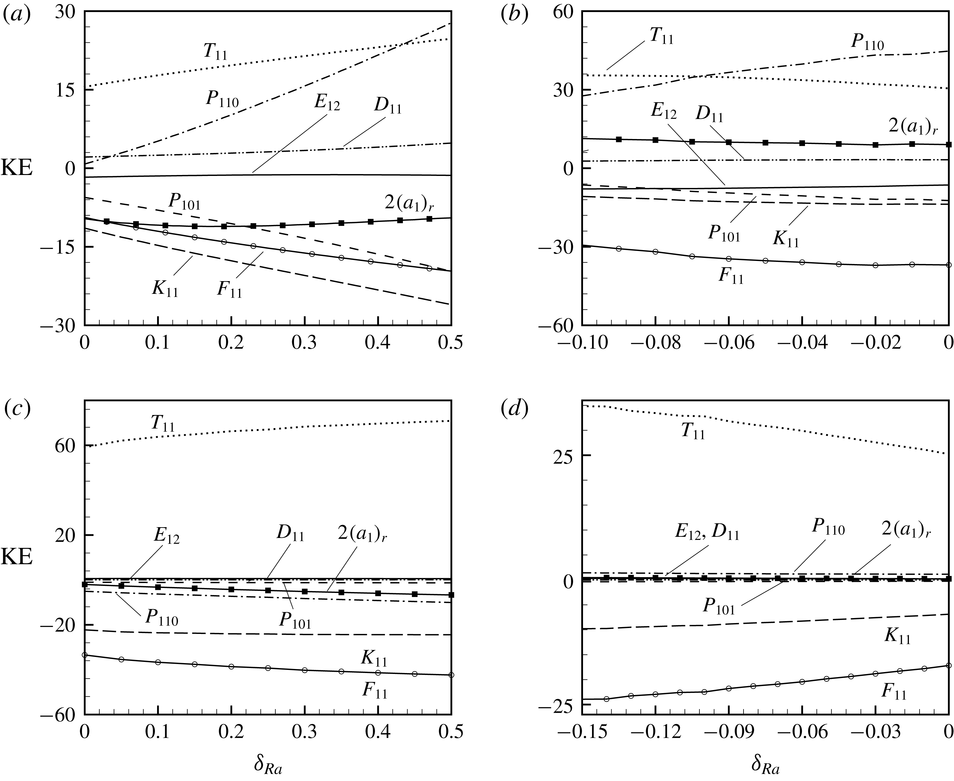
The nonlinear spectrum of KE away from the critical point for
 $Da=10^{-2}$
(
 $Da=10^{-3}$
) is shown in figure 11(a) (figure 11
c) for the supercritical regime and in figure 11(b) (figure 11
d) for the subcritical regime. The spectrum of KE in the supercritical as well as the subcritical regime for
 $Da=10^{-2}$
reveals that the three terms
 $P_{110}$
,
 $T_{11}$
and
 $D_{11}$
are positive and act as destabilizing factors. However, in the supercritical (subcritical) regime
 $T_{11}$
(
 $P_{110}$
) acts as a dominant destabilizing factor up to a certain distance from the bifurcation point. Beyond that distance,
 $P_{110}$
(
 $T_{11}$
) in the supercritical (subcritical) regime starts to play an equally important role in the KE spectrum and also becomes dominant. A notable contribution of
 $P_{110}$
in both the regimes is a consequence of the following fact. Note that in the supercritical (subcritical) regime
 $Re$
is fixed at 1000 (3000) and the basic flow has a buoyant (mixed) instability. Also, the contribution of the shear term is positive and not negligible (see discussion § 3.1). Therefore, modification to the gradient production due to a change in the shape of the fundamental wave will be more favourable for shear production. In the subcritical regime, figure 11(b) shows that the value of
 $P_{110}$
decreases as one moves down from the critical value. Since for this value of
 $Re$
the basic flow has a mixed type of instability and in the linearly stable regime the value of
 $Ra$
is less than the critical value, as a result, a relatively lower shear production is expected. Definitely the pattern of secondary flow will be influenced by this, which will be discussed in § 6.4. Furthermore, in contrast to the supercritical regime where
 $K_{11}$
,
 $F_{11}$
,
 $P_{101}$
of the disturbance KE increase on increasing
 $Ra$
, in the subcritical regime all these remain almost constant. For
 $Da=10^{-3}$
, figure 11(c,d) shows that the term
 $T_{11}$
is positive and it is the main destabilizing factor in the KE balance. The magnitude of it increases when it varies as a function of
 $Ra$
away from the critical point. Similar to figure 8(a,b) here also the term
 $P_{110}$
is negative (positive) in the supercritical (subcritical) regime. In the supercritical regime its contribution to the KE spectrum increases as it moves away from the critical point. The term
 $T_{11}$
is balanced by
 $P_{110}$
,
 $K_{11}$
and
 $F_{11}$
in the supercritical regime, whereas the same in the subcritical regime is balanced by
 $K_{11}$
and
 $F_{11}$
. Apart from these, figures 11(a,b) and 11(c,d) show that the sign of
 $2(a_{1})_{r}$
is negative (positive) in the entire supercritical regime (subcritical regime). Thus, the balance of KE supports the results obtained from the Landau constant.
6.3 Bifurcation as a function of
$\unicode[STIX]{x1D6FC}$

The variation of the neutral stability curve with wavenumber is also important because an instability that is supercritical for some wavenumber may be subcritical or supercritical at other nearby wavenumber (Rogers et al.
Reference Rogers, Moulic and Yao1993). In this situation, any of the potential unstable waves may grow and interact with other modes. Therefore, for the present problem we have chosen two different values of
 $Re$
, one from the supercritical regime and the other from the subcritical regime, for a given
 $Da$
. Accordingly, for three values
 $10^{-2}$
,
 $10^{-3}$
and
 $10^{-4}$
of
 $Da$
three different respective values 1000, 4000 and 10 000 of
 $Re$
from the supercritical regime are chosen. From the subcritical regime two values 3000 and 7000 of
 $Re$
are chosen for respectively two different values
 $10^{-2}$
and
 $10^{-3}$
of
 $Da$
.
Note that the corresponding critical points (
 $\unicode[STIX]{x1D6FC},Ra$
) for the above chosen values of
 $Re$
in the supercritical regime are (1.94, 290), (1.24, 12269) and (15.1, 137 491) and in the subcritical regime they are (1.95, 425), (1.22, 12 366), respectively. The type of instability is buoyant at all these points except for
 $Re=3000$
for
 $Da=10^{-2}$
where it is mixed or interactive. The neutral stability curves
 $(c_{i}=0)$
for different values of
 $Da$
are plotted in figure 12. Here, solid and dashed lines represent variation of
 $Ra$
with
 $\unicode[STIX]{x1D6FC}$
for a given
 $Re$
from the supercritical and subcritical regime, respectively. It can be seen from the above figure that for
 $Da=10^{-3}$
and
 $Re=7000$
(
 $Da=10^{-4}$
and
 $Re=10\,000$
), a large band of wavenumber exists in which subcritical (supercritical) bifurcation remains subcritical (supercritical). However, for
 $Da=10^{-2}$
and
 $Re=1000$
, subcritical bifurcation can be seen for
 $\unicode[STIX]{x1D6FC}<0.8$
and supercritical for
 $\unicode[STIX]{x1D6FC}>0.8$
. Similarly, for
 $Re=3000$
, supercritical bifurcation can be seen for
 $\unicode[STIX]{x1D6FC}<1.8$
and subcritical for
 $\unicode[STIX]{x1D6FC}>1.8$
. In the case of
 $Da=10^{-3}$
and
 $Re=4000$
, subcritical bifurcation can be seen for
 $\unicode[STIX]{x1D6FC}<1.12$
and supercritical for
 $\unicode[STIX]{x1D6FC}>1.12$
.
Neutral stability curve (
 $c_{i}=0$
) in the (
 $\unicode[STIX]{x1D6FC},Ra$
)-plane: (a)
 $Da=10^{-2}$
, (b)
 $Da=10^{-3}$
and (c)
 $Da=10^{-4}$
when
 $Pr=0.7$
and
 $c_{F}=6\times 10^{-3}$
.

Note that for
 $Re=4000$
the basic flow at the least linearly stable point (1.24, 12 269) is supercritically stable whereas the same at the nearby neutral point (1.1, 14 519) is subcritically unstable. Similarly, for
 $Da=10^{-2}$
the basic flow which is subcritically unstable at the least linearly stable point (1.95, 425) is supercritically stable at the nearby neutral point (1.7, 436). So, from the above analysis we can point out that with the buoyant and mixed instabilities, both subcritical and supercritical branches appear on the neutral curves.
6.4 Pattern of secondary flow
The overview of the above discussion suggests the existence of secondary flow with finite amplitude beyond the bifurcation point. We have seen that depending on the value of input parameter the bifurcation may be supercritical or subcritical. Apart from this, the balance of kinetic energy depicts a different result relative to a purely fluid domain in the supercritical regime. Therefore, the nonlinear impact on secondary flow from the linearly least stable wave is analysed in the supercritical as well as the subcritical regime. The secondary flow under linear stability analysis is obtained from the eigenfunction associated with the linearly least stable eigenvalue and the same from the weakly nonlinear analysis is calculated as a superposition of different harmonics (here,
 $E^{1}$
and
 $E^{2}$
in (4.1)). Following Khandelwal & Bera (Reference Khandelwal and Bera2015), the functions
 $\hat{u} _{1}$
,
 $\hat{u} _{2}$
, etc., for the secondary flow are calculated. The eigenfunction includes the disturbance
 $u$
and
 $v$
velocities as well as disturbance temperature (
 $\unicode[STIX]{x1D703}$
). However, to avoid numerous figures the pattern of disturbance of the
 $v$
velocity is not shown in the following. We are interested in studying the pattern of secondary flow very close to the bifurcation point as well as away from the bifurcation point under linear and weakly nonlinear analyses.
We restrict our analysis to the same four pairs (
 $10^{-2},1000$
), (
 $10^{-3},4000$
), (
 $10^{-2},3000$
) and (
 $10^{-3},7000$
) of (
 $Da,Re$
) which are also used in § 6.2. As discussed therein,
 $\unicode[STIX]{x1D6FF}_{Ra}=0.01$
and
 $\unicode[STIX]{x1D6FF}_{Ra}=0.5$
are points from the supercritical regime for the first two pairs of (
 $Da,Re$
), whereas
 $\unicode[STIX]{x1D6FF}_{Ra}=-0.01$
and
 $\unicode[STIX]{x1D6FF}_{Ra}=-0.5$
are points from the subcritical regime for the last pair of (
 $Da,Re$
) only. Since the subcritical regime of
 $(Da,Re)=(10^{-2},3000)$
is
 $0\geqslant \unicode[STIX]{x1D6FF}_{Ra}\geqslant -0.1$
, for this pair of
 $(Da,Re)$
,
 $\unicode[STIX]{x1D6FF}_{Ra}=-0.01$
and
 $\unicode[STIX]{x1D6FF}_{Ra}=-0.1$
are chosen as respective points from very close to the critical point and away from the critical point. In the following the solid and dashed lines in the contours are associated with respective positive and negative values of a field variable.
Pattern of secondary flow by (a) linear stability analysis and (b) nonlinear stability analysis when
 $Da=10^{-2}$
,
 $Pr=0.7$
,
 $Re=1000$
and
 $\unicode[STIX]{x1D6FF}_{Ra}=0.01$
as well as
 $\unicode[STIX]{x1D6FF}_{Ra}=0.5$
: (i) and (iii) disturbance
 $u$
-velocity; (ii) and (iv) disturbance temperature.
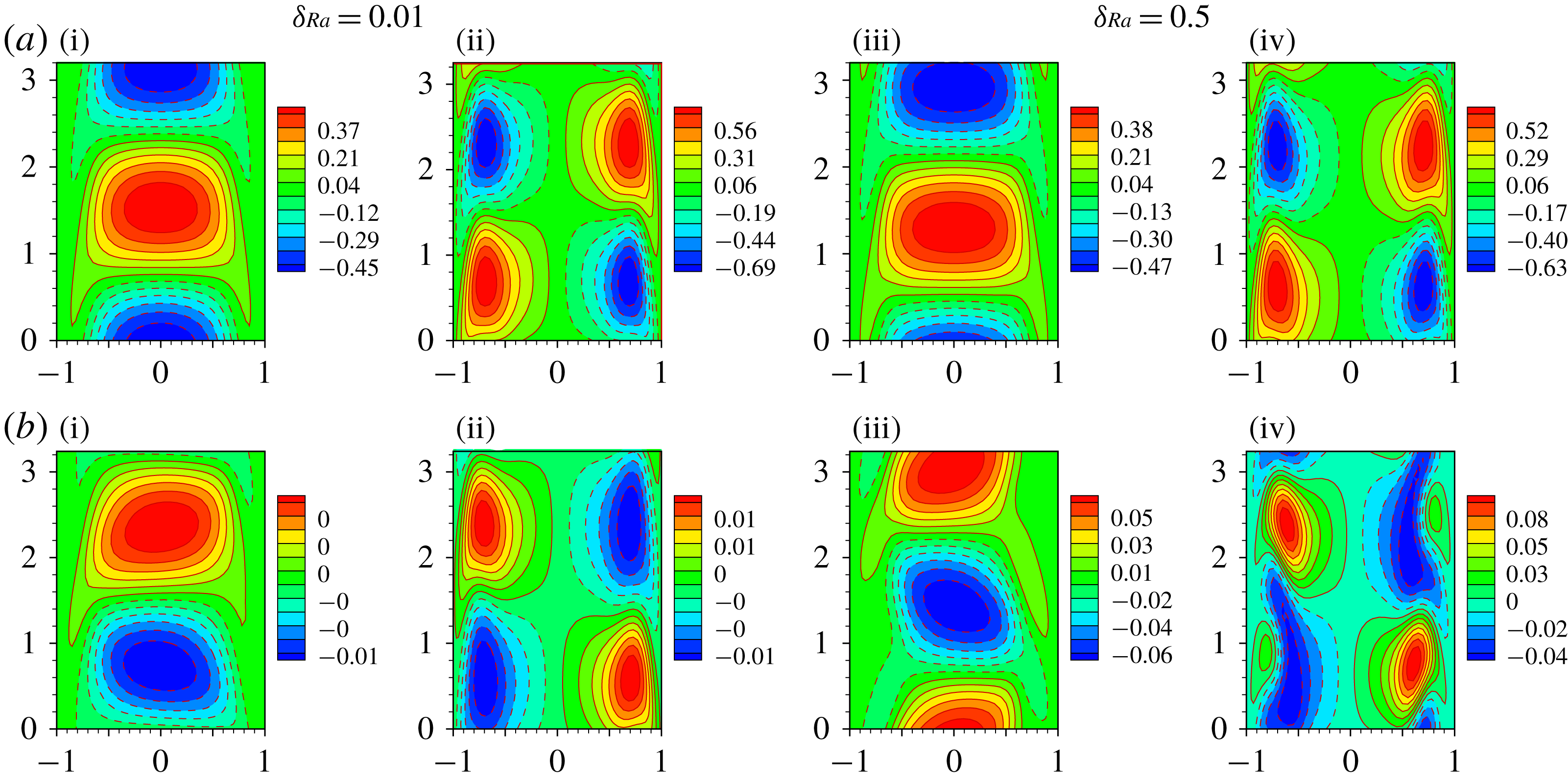
Pattern of secondary flow by (a) linear stability analysis and (b) nonlinear stability analysis when
 $Da=10^{-3}$
,
 $Pr=0.7$
,
 $Re=4000$
and
 $\unicode[STIX]{x1D6FF}_{Ra}=0.01$
as well as
 $\unicode[STIX]{x1D6FF}_{Ra}=0.5$
: (i) and (iii) disturbance
 $u$
-velocity; (ii) and (iv) disturbance temperature.
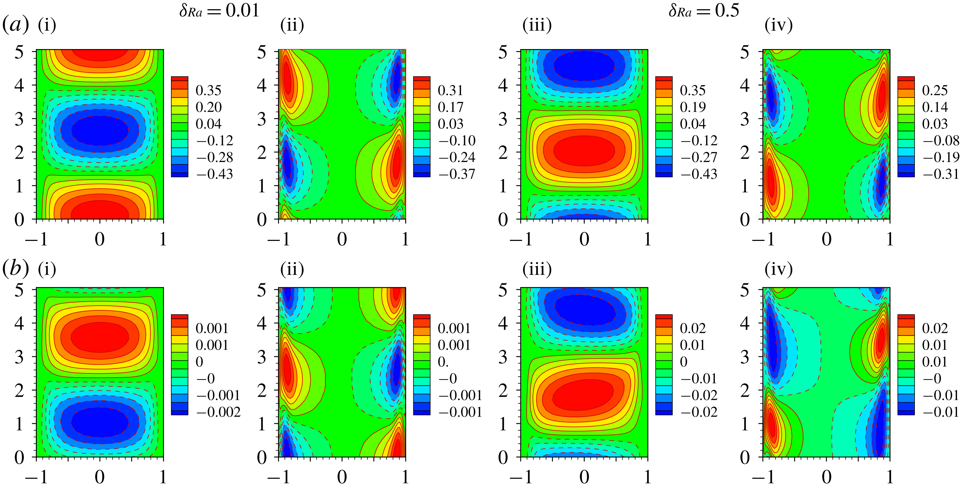
Pattern of secondary flow by (a) linear stability analysis and (b) nonlinear stability analysis when
 $Da=10^{-2}$
,
 $Pr=0.7$
,
 $Re=3000$
and
 $\unicode[STIX]{x1D6FF}_{Ra}=-0.01$
as well as
 $\unicode[STIX]{x1D6FF}_{Ra}=-0.1$
: (i) and (iii) disturbance
 $u$
-velocity; (ii) and (iv) disturbance temperature.
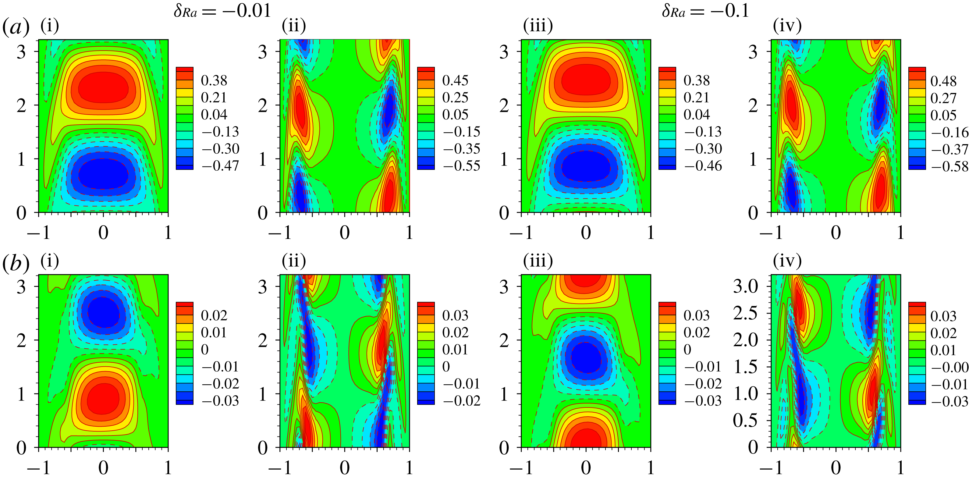
Pattern of secondary flow by (a) linear stability analysis and (b) nonlinear stability analysis when
 $Da=10^{-2}$
,
 $Pr=0.7$
,
 $Re=2000$
and
 $\unicode[STIX]{x1D6FF}_{Ra}=-0.01$
as well as
 $\unicode[STIX]{x1D6FF}_{Ra}=-0.1$
: (i) and (iii) disturbance
 $u$
-velocity; (ii) and (iv) disturbance temperature.
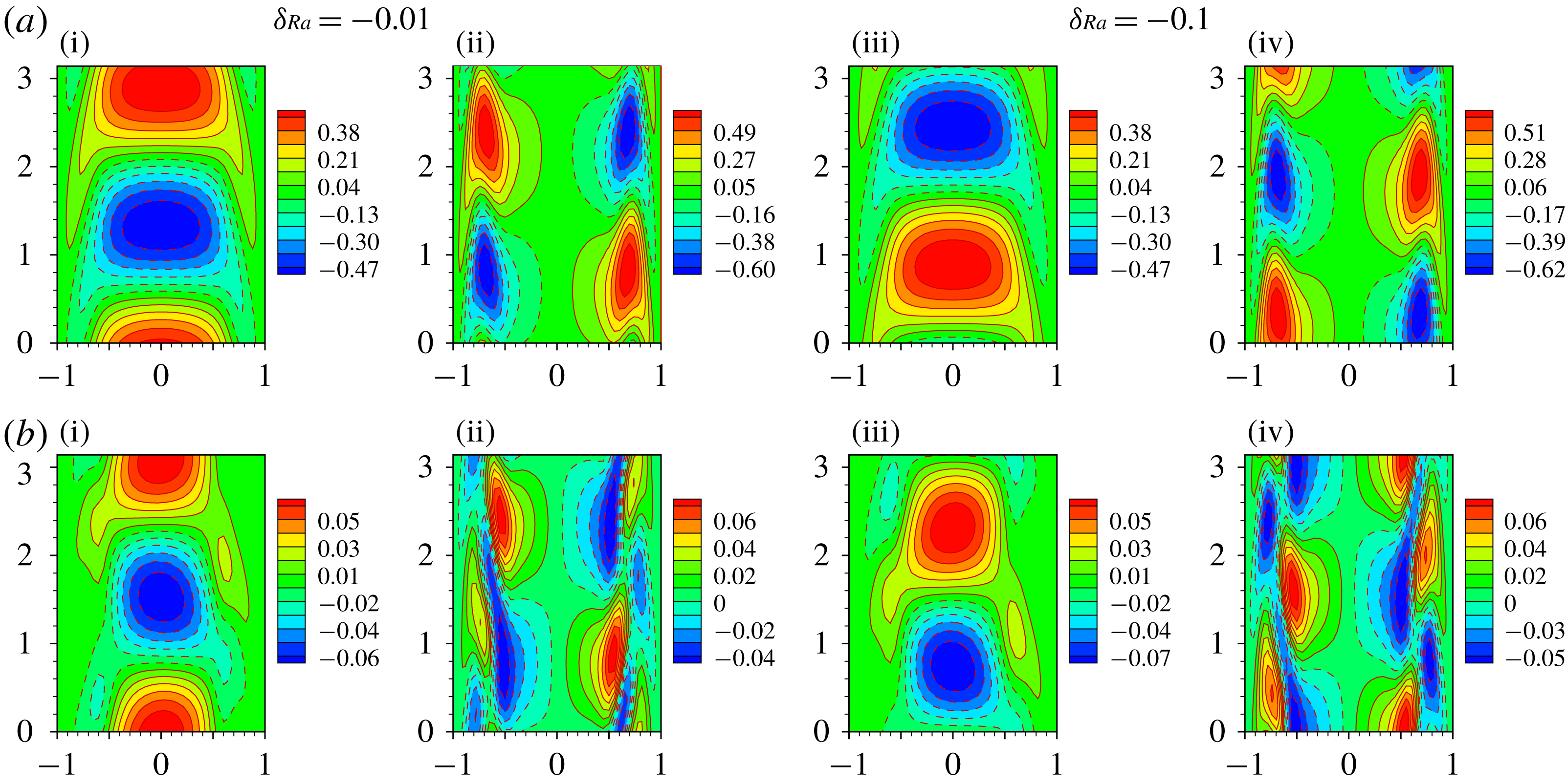
Pattern of secondary flow by (a) linear stability analysis and (b) nonlinear stability analysis when
 $Da=10^{-3}$
,
 $Pr=0.7$
,
 $Re=7000$
and
 $\unicode[STIX]{x1D6FF}_{Ra}=-0.01$
as well as
 $\unicode[STIX]{x1D6FF}_{Ra}=-0.5$
: (i) and (iii) disturbance
 $u$
-velocity; (ii) and (iv) disturbance temperature.
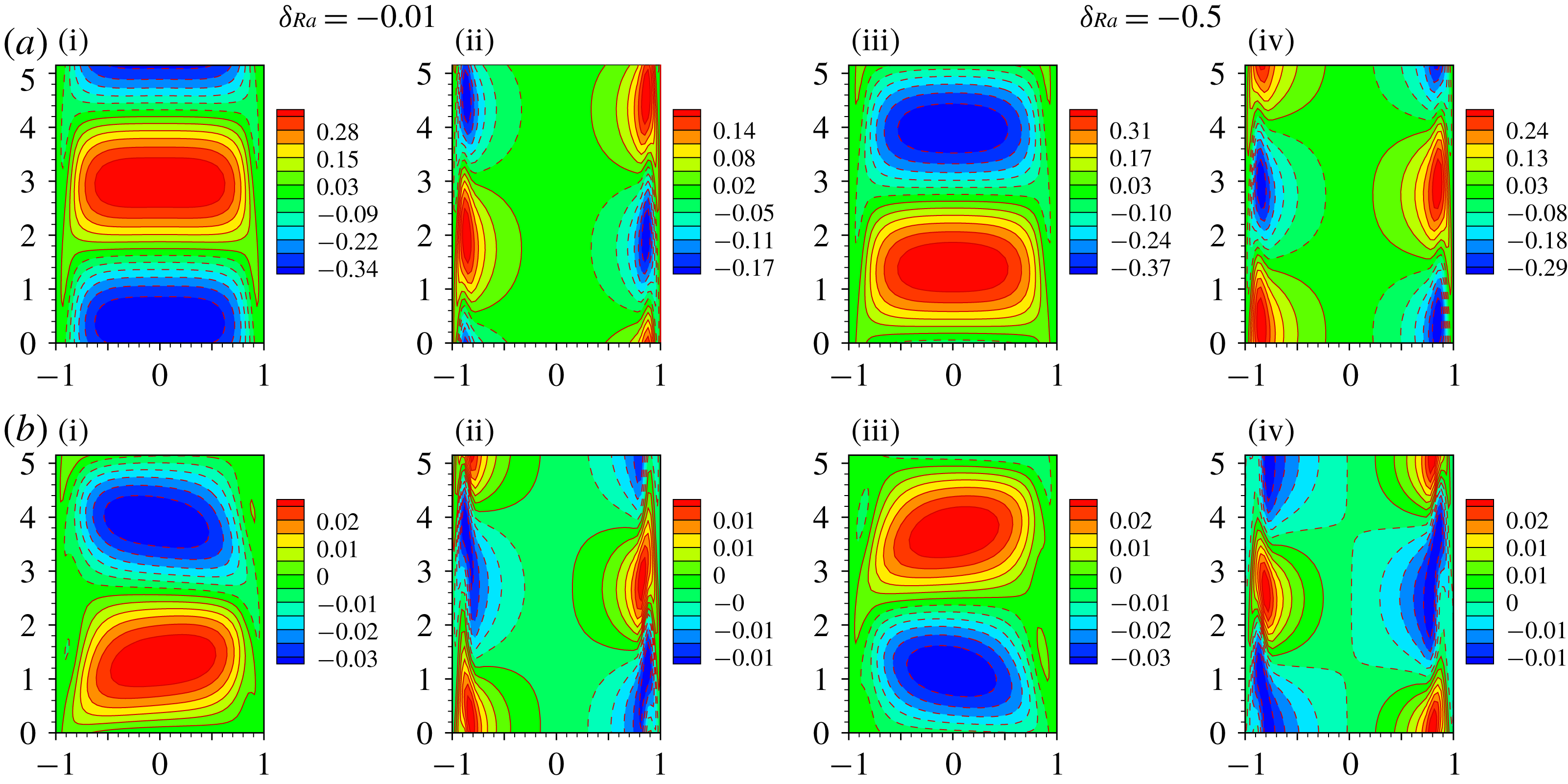
The patterns of secondary flow in the supercritical regime, when
 $Re=1000$
and
 $Da=10^{-2}$
, from linear stability theory and weakly nonlinear stability theory are shown in figures 13(a) and 13(b), respectively. As can be seen from the above figures, the difference between the patterns of secondary flow using linear and weakly nonlinear theories at
 $\unicode[STIX]{x1D6FF}_{Ra}=0.01$
is negligible as compared to the same at
 $\unicode[STIX]{x1D6FF}_{Ra}=0.5$
. However, magnitude-wise it differs significantly for both values of
 $\unicode[STIX]{x1D6FF}_{Ra}$
. Apart from these, although the shape of the contours of the disturbance temperature and the
 $u$
-velocity in the linear stability analysis are deformed significantly under the nonlinear analysis, the deformation in the disturbance temperature is much higher than the same in the disturbance velocity. It increases as one moves away from the bifurcation point. This type of modification in the fundamental disturbance is also predicted in the energy analysis in § 6.2. To check the above result for other values of
 $Da$
we have plotted the same for
 $Da=10^{-3}$
when
 $Re=4000$
in figures 14(a) and 14(b), respectively. Although these also give a similar impression, compared to
 $(Da,Re)=(10^{-2},3000)$
the change of shape in the disturbance velocity as well as the temperature under the nonlinear analysis for the considered pair of
 $(Da,Re)$
is less. Here, at
 $\unicode[STIX]{x1D6FF}_{Ra}=0.01$
the deformation of the contours is mainly in terms of shifting.
In the subcritical regime for
 $Da=10^{-2}$
, figure 15(a,b) shows that the deformation of the fundamental disturbance, in the vicinity of the bifurcation point, is much higher than the same under the supercritical regime. Here, the deformation of the cells is in the form of shifting as well as stretching. The deformation of the fundamental disturbance under nonlinear interaction in the neighbourhood of the
 $Re_{sb}$
is expected to be much more than the same far away from
 $Re_{sb}$
. Therefore, figures 16(a) and 16
b) are drawn for
 $Re=2000$
and
 $Da=10^{-2}$
. Note that for
 $Re=2000$
the calculated subcritical regime is
 $-0.12\leqslant \unicode[STIX]{x1D6FF}_{Ra}\leqslant 0$
. As can be seen from figure 16(a,b), the above expectation is correct. The shape of the uni-cellular structure of the
 $u$
velocity from linear stability theory shifts to a deformed multicellular structure for
 $\unicode[STIX]{x1D6FF}_{Ra}=-0.1$
. Deformation of the temperature cells under subcritical bifurcation is accelerated as one moves away from the bifurcation point. In order to cross-check the pattern variation of secondary flow in the subcritical regime when
 $Da$
is changed to
 $10^{-3}$
, figure 18 is drawn for
 $Re=7000$
. Here, deformation of the fundamental disturbance under nonlinear interaction is much less as compared to
 $Da=10^{-2}$
at both values
 $-0.01$
and
 $-0.5$
of
 $\unicode[STIX]{x1D6FF}_{Ra}$
, which is also expected from the nonlinear energy spectrum.
From the above analysis, we would like to mention that a jump in the amplitude profile of a physical problem, which was observed in §§ 6.1 and 6.2, leads to a transition from supercritical bifurcation to subcritical bifurcation or vice versa and deforms the pattern of secondary flow under linear stability analysis significantly (see figures 15 and 16).
7 Conclusion
This study considers the weakly nonlinear stability analysis of stably stratified PMCF of air as well as water in a vertical channel filled with a porous medium. The purpose of this study is to analyse the nature of bifurcation and the finite amplitude behaviour of unstable disturbances that occur beyond the linear instability boundary, especially when the permeability of the medium and strength of the flow are reasonably high. This is accomplished by reviewing the linear stability results, and then a weakly nonlinear analysis is undertaken to trace the evolution of the finite amplitude perturbation. We have analysed that, based on the value of
 $Da$
, for lower values of
 $Re$
the critical value of the Rayleigh number decreases with increasing Reynolds number and there may be a minimum value of
 $Re$
above which the curve will have an increasing characteristic. This may continue further up to a certain value of
 $Re$
and beyond that it may asymptotically converge to a constant.
To study the evolution of the finite amplitude perturbation, we have started by analysing the variation of the real part of the Landau constant (
 $(a_{1})_{r}$
) and the amplitude in the vicinity of the least linearly stable point as a function of
 $Re$
for air as well as water. Depending on the flow strength as well as the medium’s permeability, the weakly nonlinear analysis predicts both supercritical and subcritical bifurcations for air, and only supercritical bifurcation for water. For an air-saturated porous medium it also predicts the possibility of existence of a minimum value of
 $Re$
, which is defined as
 $Re_{sb}$
such that in its vicinity, change of sign of
 $(a_{1})_{r}$
takes place and gives an indication of a shifting of the bifurcation. Increase in the form drag coefficient or a decrease in the medium’s permeability, in general, delays the shifting of the bifurcation from supercritical to subcritical or vice versa in the (
 $(a_{1})_{r},Re$
)-plane. Compared to subcritical bifurcation, the supercritical bifurcation occurs at relatively lower values of
 $Re$
. The amplitude profile shows a jump in the vicinity of
 $Re_{sb}$
, due to a change in sign of
 $(a_{1})_{r}$
. The similar characteristic is also reflected in the physical quantities such as distorted Nusselt number and friction coefficient. Furthermore, based on very small value of
 $c_{i}$
, we have analysed the bifurcation away from the critical point for particular choices of
 $Re$
in the supercritical as well as subcritical bifurcation regime. It has been found that, depending on the value of
 $Da$
, a subcritical flow in linearly stable regime may change to a supercritical one in the linearly unstable regime and vice versa. Subcritical bifurcation in the linearly stable regime yields a lower critical value, below which the bifurcated solution does not exist. For example, when
 $Da=10^{-3}$
the critical values of
 $Ra$
for two values, 4000 and 7000, of
 $Re$
are 12 269 and 12 366, respectively, whereas the corresponding probable lower critical values are 4907.6 and 6183, respectively. In the linearly unstable regime, due to nonlinear interaction of different harmonics, the heat transfer rate (skin friction) increases (decreases) significantly, whereas the same in the linearly stable regime is almost negligible.
Through linear as well as nonlinear energy analysis it has been found that in supercritical as well as subcritical regimes, due to a change in the shape of the fundamental disturbance wave,
 $T_{11}$
is the main destabilizing factor and
 $K_{11}$
as well as
 $F_{11}$
are the main stabilizing factors when
 $Da=10^{-3}$
. Although,
 $P_{110}$
is not favourable for shear production in the linearly unstable regime for
 $Da=10^{-3}$
, for
 $Da=10^{-2}$
it is favourable for shear production in the linearly unstable as well as stable regimes. For this value of
 $Da$
, except in the vicinity of the bifurcation point, both
 $T_{11}$
and
 $P_{110}$
act as major destabilizing terms in the KE balance. It has been also seen that when the shear term in the linear KE balance is in favour of destabilizing the flow in that situation,
 $P_{110}$
, in the nonlinear KE spectrum, also acts as a destabilizing term, and the reverse is not true.
It is important to mention here that Rogers et al. (Reference Rogers, Moulic and Yao1993), while studying mixed convection flow in a vertical annulus, have found the supercritical bifurcation at all wavenumbers for thermal–shear instability flow, whereas for a flow with an interactive (mixed) instability, both subcritical and supercritical branches appear on the neutral curves. The present study reveals that both subcritical and supercritical branches may appear on the neutral curves for buoyant as well as interactive (mixed) instabilities. Finally, the pattern variation of the secondary flow is also analysed to cross-check the prediction made through nonlinear energy balance towards the possible variation of shape of the fundamental disturbance under nonlinear interaction of different harmonics. It has been found that the prediction made through energy analysis is correct.
The details of the finite amplitude stability analysis for PMCF in a vertical porous medium channel are of much interest. Although we have explored some important features including types of bifurcations, energy transfer and secondary flow, the findings can also be viewed in the broader context of the stability behaviour of the present flow with the help of a higher-order weakly nonlinear stability analysis and direct numerical simulation. These analyses are left for our future study.
Acknowledgements
This work is partially supported by the Department of Science and Technology (DST) Project grant no. SER-778-MTD of India. One of the authors A.K.S. is also grateful to MHRD India for providing financial support during the preparation of this manuscript. We are indebted to anonymous reviewers for their suggestions and remarks in light of which we could improve the article.
Appendix A. A note about model equations
Due to lack of a unified theory for transport in porous media, different models have emerged based on empirical results (i.e. experimental data) as well as different theoretical approaches (i.e. volume-averaged analysis, matched asymptotic expansion, etc.). The volume-averaged Navier–Stokes (VANS) equation derived by Whitaker (Reference Whitaker1996) for an incompressible viscous fluid flowing through a rigid, homogeneous, isotropic, porous medium is of the form
 $$\begin{eqnarray}\displaystyle \unicode[STIX]{x1D70C}_{f}\left[\frac{1}{\unicode[STIX]{x1D700}}\frac{\unicode[STIX]{x2202}\boldsymbol{v}}{\unicode[STIX]{x2202}t}+\frac{1}{\unicode[STIX]{x1D700}^{2}}\boldsymbol{v}\boldsymbol{\cdot }\unicode[STIX]{x1D735}\boldsymbol{v}+c_{F}K^{-1/2}|\boldsymbol{v}|\boldsymbol{v}\right]=-\unicode[STIX]{x1D735}P+\unicode[STIX]{x1D70C}g\boldsymbol{e}_{\boldsymbol{y}}+\widetilde{\unicode[STIX]{x1D707}}\unicode[STIX]{x1D6FB}^{2}\boldsymbol{v}-\unicode[STIX]{x1D707}_{f}\frac{\boldsymbol{v}}{K}, & & \displaystyle\end{eqnarray}$$
where
 $\boldsymbol{v}$
is the Darcy velocity,
 $P$
is the pressure,
 $\unicode[STIX]{x1D700}$
is the porosity of the medium,
 $c_{F}$
is the form drag coefficient,
 $K$
is the permeability of the porous medium,
 $\text{g}$
is gravitational acceleration,
 $\widetilde{\unicode[STIX]{x1D707}}$
is the effective viscosity,
 $\unicode[STIX]{x1D707}_{f}$
is the fluid viscosity,
 $\unicode[STIX]{x1D70C}_{f}$
is fluid density,
 $\unicode[STIX]{x1D70C}$
is fluid density given by equation of state and
 $\boldsymbol{e}_{\boldsymbol{y}}$
is a unit vector in the
 $y$
-direction. In this equation, the Darcy term (
 $\unicode[STIX]{x1D707}_{f}\boldsymbol{v}/K$
) represents a volume-averaged viscous drag, the Brinkman term (
 $\widetilde{\unicode[STIX]{x1D707}}\unicode[STIX]{x1D6FB}^{2}\boldsymbol{v}$
) represents a volume-averaged viscous diffusion, the Forchheimer term (
 $c_{F}K^{-1/2}|\boldsymbol{v}|\boldsymbol{v}$
) represents form drag due to inertial effects and the convective term (
 $\unicode[STIX]{x1D70C}_{f}\boldsymbol{v}\boldsymbol{\cdot }\unicode[STIX]{x1D735}\boldsymbol{v}/\unicode[STIX]{x1D700}^{2}$
) represents another drag which arises from inertial effects. It is important to mention that volume averaging the convective term in the Navier–Stokes equation generates the terms
 $\unicode[STIX]{x1D70C}_{f}\boldsymbol{v}\boldsymbol{\cdot }\unicode[STIX]{x1D735}\boldsymbol{v}/\unicode[STIX]{x1D700}^{2}$
and
 $c_{F}K^{-1/2}|\boldsymbol{v}|\boldsymbol{v}$
when the difference between the velocity of fluid and the volume average velocity of the fluid is negligible. Whitaker (Reference Whitaker1996) found that the contribution of the convective term
 $\unicode[STIX]{x1D70C}_{f}\boldsymbol{v}\boldsymbol{\cdot }\unicode[STIX]{x1D735}\boldsymbol{v}/\unicode[STIX]{x1D700}^{2}$
is negligible in comparison with the dominant Forchheimer term,
 $c_{F}K^{-1/2}|\boldsymbol{v}|\boldsymbol{v}$
. However, without a convective term, there is no mechanism for development of the flow field, which leads to a physically flawed and unrealistic situation (Vafai & Kim Reference Vafai and Kim1995). The literature review reveals some inconsistencies in the proper form of the equations governing the flow through porous media (Whitaker Reference Whitaker1996; Giorgi Reference Giorgi1997; Lage Reference Lage, Ingham and Pop1998) but the form of equation by the volume-averaged method is particularly useful in channel flow (Tilton & Cortelezzi Reference Tilton and Cortelezzi2008; Zhang et al.
Reference Zhang, Li and Nakayamayao2015). Note that Vafai & Tien (Reference Vafai and Tien1981) as well as Hsu & Cheng (Reference Hsu and Cheng1990) have also used the volume-averaging concept to derive porous flow equations similar to the above equation. Without diminishing the importance of their work, we also prefer the derivation of Whitaker (Reference Whitaker1996) because it is, to the best of our knowledge, the most complete and formal.
The contribution of different terms to the above equation depends mainly on (i) the type of porous medium in which fluid flow is considered and (ii) the nature and strength of the flow. The Darcy model is limited to describing the fluid flow in a porous medium when the Darcy velocity is small. It does not satisfy the no-slip condition. To investigate the dynamics of pressure-driven flow in a channel, the Brinkman term is required to satisfy the no-slip condition (Tilton & Cortelezzi Reference Tilton and Cortelezzi2008). Furthermore, if the porous medium is made of metallic foam then the Forchheimer extended Darcy law is valid for most of the metal foams (Zhang et al.
Reference Zhang, Li and Nakayamayao2015). If the permeability of the medium is high and strength of the forced flow is also reasonably high then the contribution of
 $\unicode[STIX]{x1D70C}_{f}\boldsymbol{v}\boldsymbol{\cdot }\unicode[STIX]{x1D735}\boldsymbol{v}/\unicode[STIX]{x1D700}^{2}$
is expected in evaluating the instability boundary point or critical point of a basic flow. In this context a rigorous study is already reported by Kumar et al. (Reference Kumar, Bera and Khalili2010). The authors have shown that if the permeability of the medium is not high then the results (i.e. instability boundary curve) from a model containing the Darcy and Brinkman terms and a model containing the Darcy, Brinkman and Forchheimer terms are the same. Also, in this situation, results from a model containing the Darcy, Brinkman and convective terms and a model containing Darcy, Brinkman, convective and Forchheimer terms are the same. They have also shown that all four models give almost the same result when the fluid is water. Apart from these, while studying the effect of particle size of the porous medium on forced convection from a circular cylinder without assuming local thermal equilibrium between phases, Al-Sumaily et al. (Reference Al-Sumaily, Nakayama, Sheridan and Thompson2012) have shown that the model containing all four terms mentioned above gives a very good approximation to the experimental results of Nasr, Ramadhyani & Viskanta (Reference Nasr, Ramadhyani and Viskanta1994). The appropriateness of inclusion of different terms in the momentum equation is still a matter of vital discussion in the literature.
Appendix B.
B.1 Basic flow profiles
The basic velocity profiles for different
 $Da$
at
 $c_{F}=6\times 10^{-3}$
and
 $c_{F}=6\times 10^{-2}$
are shown in figures 18(a) and 18(b), respectively. As can be seen from the figures, for each considered value of
 $Da$
as well as
 $c_{F}$
, the velocity profile contains a point of inflection for
 $Ra=500$
, which is consequence of (i) the no-slip condition on the wall, (ii) acceleration of fluid near the wall due to the buoyant term and (iii) deceleration of the colder fluid near the centre due to mass conservation. The point of inflection shifts towards the walls on decreasing the value of
 $Da$
as well as increasing the value of
 $c_{F}$
. Appearance of an inflection point indicates a potential for instability.
Basic velocity profile for different
 $Da$
: (a)
 $c_{F}=6\times 10^{-3}$
, (b)
 $c_{F}=6\times 10^{-2}$
, when
 $Ra=500$
and
 $Re=1000$
.
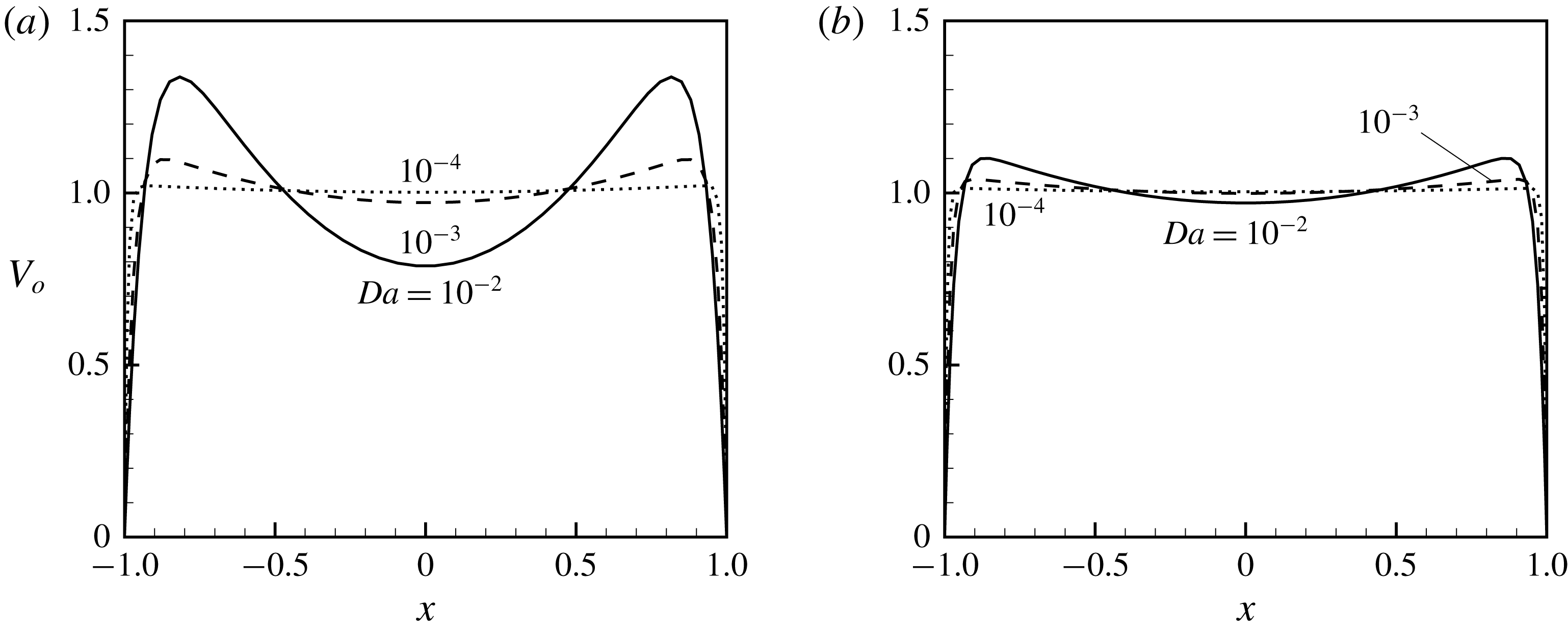
B.2 Growth rate of disturbance
The growth rate as a function of
 $Re$
for
 $c_{F}=6\times 10^{-4}$
, and
 $c_{F}=6\times 10^{-3}$
is shown in figures 19(a) and 19(b), respectively. As can be seen, based on the value of
 $c_{F}$
, the growth rate decreases up to a certain value of
 $Re$
and beyond that it increases marginally. Growth rate is positive and non-zero.
The growth rate as a function of
 $Ra$
in the supercritical and subcritical regimes of
 $Re$
is shown in figures 20(a) and 20(b), respectively. The critical points (
 $\unicode[STIX]{x1D6FC},Ra$
) for two values, 1000 and 3000, of
 $Re$
for
 $Da=10^{-2}$
are (1.94, 290) and (1.95, 425), respectively. The same for two values 4000 and 7000 of
 $Re$
for
 $Da=10^{-3}$
are (1.24, 12 269) and (1.22, 12 366), respectively. Both figures show the validity of linear variation of growth rate away from the critical point for both values of
 $10^{-2}$
and
 $10^{-3}$
of
 $Da$
.
Variation of growth rate (
 $\unicode[STIX]{x1D6FC}c_{i}$
) as a function of
 $Re$
, when
 $Da=10^{-3}$
and
 $Pr=0.7$
: (a)
 $c_{F}=6\times 10^{-4}$
, (b)
 $c_{F}=6\times 10^{-3}$
. The solid line (dashed line) represents the growth rate at
 $\unicode[STIX]{x1D6FF}_{Ra}=0.01~(-0.01)$
.
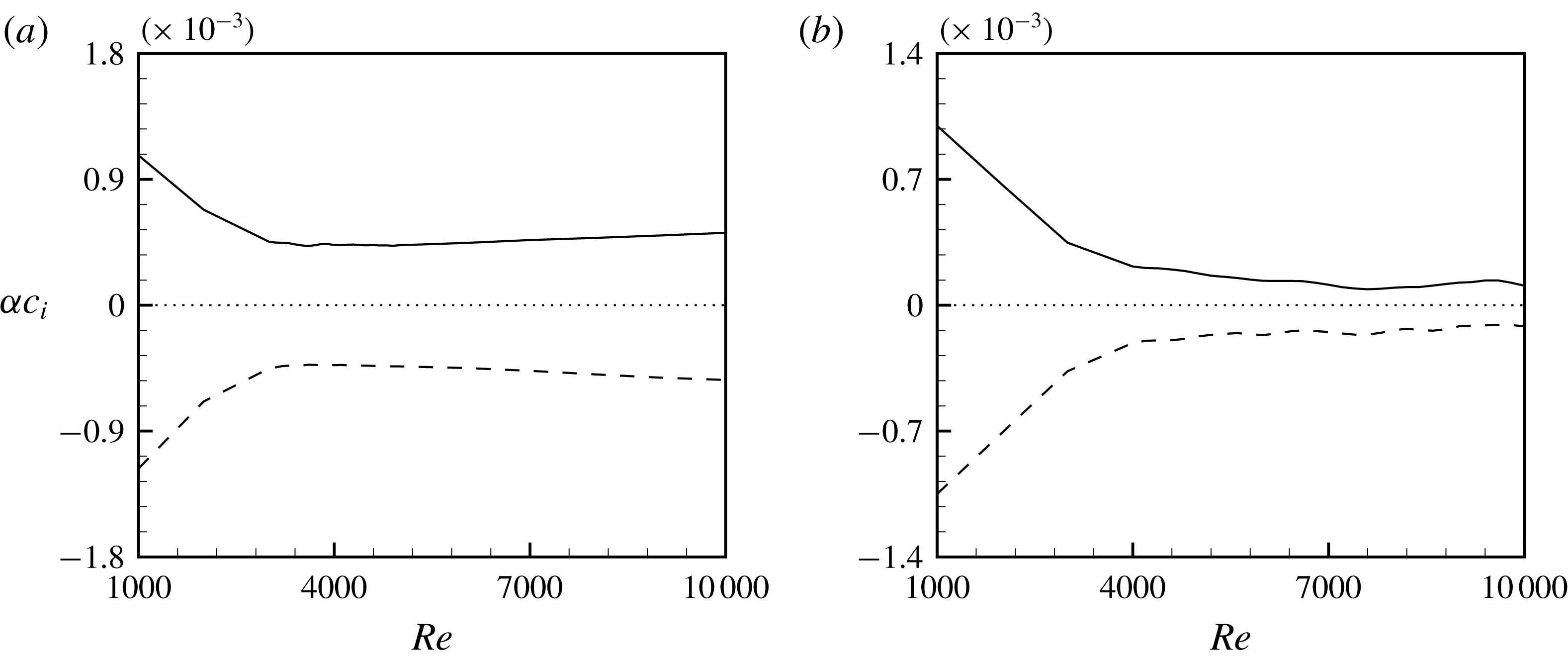
Variation of growth rate (
 $\unicode[STIX]{x1D6FC}c_{i}$
) as a function of
 $\unicode[STIX]{x1D6FF}_{Ra}$
when
 $Pr=0.7$
.
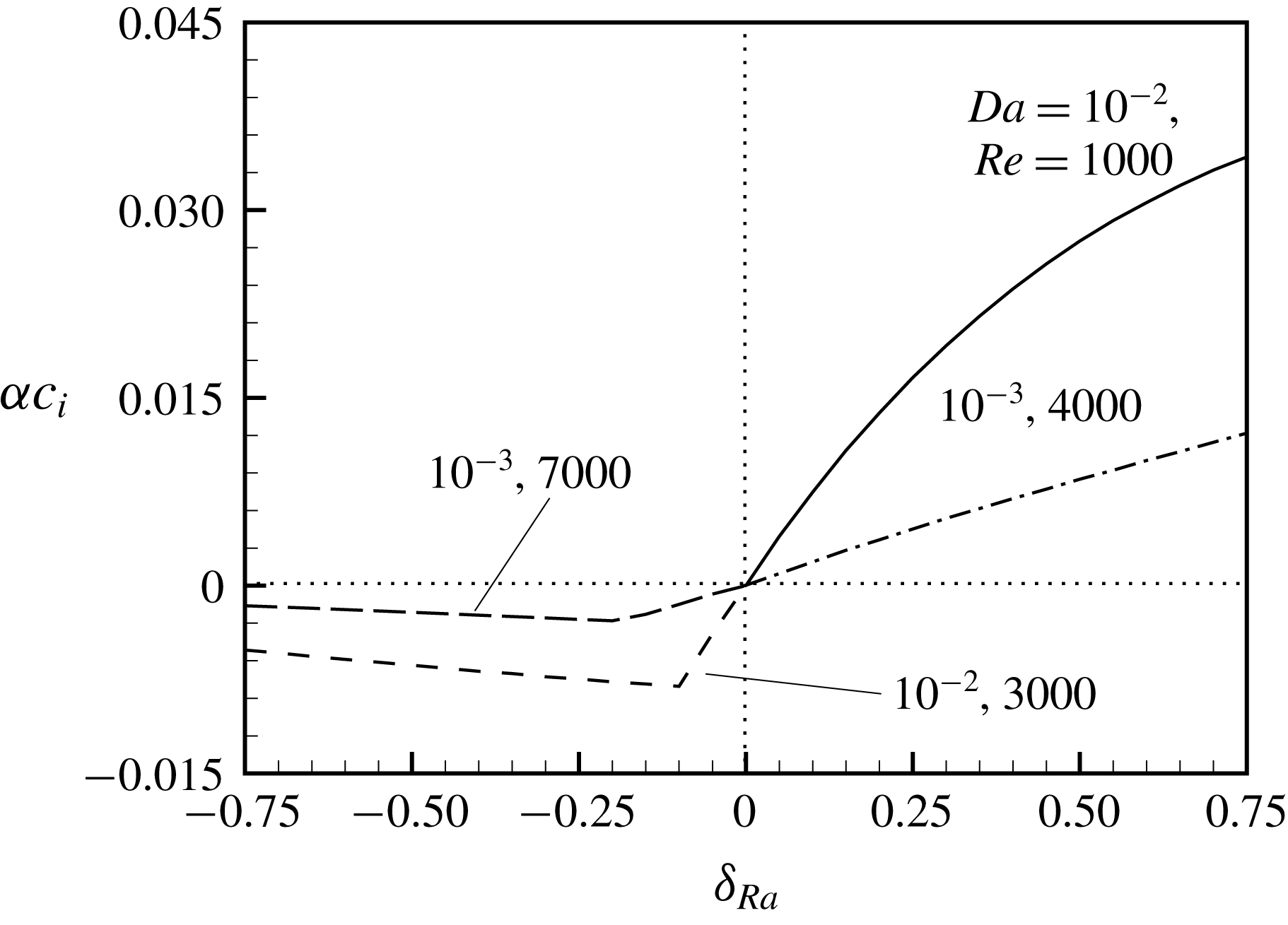
Appendix C.
C.1 Linear disturbance equations
 $$\begin{eqnarray}\displaystyle \mathscr{L}_{o}(\unicode[STIX]{x1D6FC},\unicode[STIX]{x1D6FD},\hat{u} ,\hat{v},{\hat{w}})=\frac{\text{d}\hat{u} }{\text{d}x}+\text{i}\unicode[STIX]{x1D6FC}\hat{v}+\text{i}\unicode[STIX]{x1D6FD}{\hat{w}}=0, & & \displaystyle\end{eqnarray}$$
 $$\begin{eqnarray}\displaystyle \mathscr{L}_{x}(\unicode[STIX]{x1D6FC},\unicode[STIX]{x1D6FD},c,\hat{u} ,\hat{p},V_{0},Da,F,Re) & = & \displaystyle \text{i}\unicode[STIX]{x1D6FC}Re\frac{1}{\unicode[STIX]{x1D700}}\left(\frac{1}{\unicode[STIX]{x1D700}}V_{0}-c\right)\hat{u} -\unicode[STIX]{x1D706}\left(\frac{\text{d}^{2}\hat{u} }{\text{d}x^{2}}-(\unicode[STIX]{x1D6FC}^{2}+\unicode[STIX]{x1D6FD}^{2})\hat{u} \right)\nonumber\\ \displaystyle & & \displaystyle +\,Re\frac{\text{d}\hat{p}}{\text{d}x}+\frac{1}{Da}\hat{u} +F^{\prime }|V_{0}|\hat{u} =0,\end{eqnarray}$$
 $$\begin{eqnarray}\displaystyle & & \displaystyle \mathscr{L}_{y}(\unicode[STIX]{x1D6FC},\unicode[STIX]{x1D6FD},c,\hat{u} ,\hat{v},\hat{p},\hat{\unicode[STIX]{x1D703}},V_{0},Ra,Da,F,Re)\nonumber\\ \displaystyle & & \displaystyle \quad =\text{i}\unicode[STIX]{x1D6FC}Re\frac{1}{\unicode[STIX]{x1D700}}\left(\frac{1}{\unicode[STIX]{x1D700}}V_{0}-c\right)\hat{v}-\unicode[STIX]{x1D706}\left(\frac{\text{d}^{2}\hat{v}}{\text{d}x^{2}}-(\unicode[STIX]{x1D6FC}^{2}+\unicode[STIX]{x1D6FD}^{2})\hat{v}\right)\nonumber\\ \displaystyle & & \displaystyle \qquad +\,\text{i}\unicode[STIX]{x1D6FC}Re\hat{p}+Re\frac{1}{\unicode[STIX]{x1D700}^{2}}\frac{\text{d}V_{0}}{\text{d}x}\hat{u} +\frac{1}{Da}\hat{v}+2F^{\prime }|V_{0}|\hat{v}-Ra\hat{\unicode[STIX]{x1D703}}=0,\end{eqnarray}$$
 $$\begin{eqnarray}\displaystyle \mathscr{L}_{z}(\unicode[STIX]{x1D6FC},\unicode[STIX]{x1D6FD},c,{\hat{w}},\hat{p},V_{0},Da,F,Re) & = & \displaystyle \text{i}\unicode[STIX]{x1D6FC}Re\frac{1}{\unicode[STIX]{x1D700}}\left(\frac{1}{\unicode[STIX]{x1D700}}V_{0}-c\right){\hat{w}}-\unicode[STIX]{x1D706}\left(\frac{\text{d}^{2}{\hat{w}}}{\text{d}x^{2}}-(\unicode[STIX]{x1D6FC}^{2}+\unicode[STIX]{x1D6FD}^{2}){\hat{w}}\right)\nonumber\\ \displaystyle & & \displaystyle +\,\text{i}\unicode[STIX]{x1D6FD}Re\hat{p}+\frac{1}{Da}{\hat{w}}+F^{\prime }|V_{0}|{\hat{w}}=0,\end{eqnarray}$$
 $$\begin{eqnarray}\displaystyle \mathscr{L}(\unicode[STIX]{x1D6FC},\unicode[STIX]{x1D6FD},c,\hat{u} ,\hat{v},\hat{\unicode[STIX]{x1D703}},V_{0},\unicode[STIX]{x1D6E9}_{0}) & = & \displaystyle -\text{i}\unicode[STIX]{x1D6FC}PrRe(V_{0}-\unicode[STIX]{x1D70E}c)\hat{\unicode[STIX]{x1D703}}+\left(\frac{\text{d}^{2}\hat{\unicode[STIX]{x1D703}}}{\text{d}x^{2}}-(\unicode[STIX]{x1D6FC}^{2}+\unicode[STIX]{x1D6FD}^{2})\hat{\unicode[STIX]{x1D703}}-\hat{v}\right)\nonumber\\ \displaystyle & & \displaystyle -\,PrRe\frac{\text{d}\unicode[STIX]{x1D6E9}_{0}}{\text{d}x}\hat{u} =0.\end{eqnarray}$$
C.2 Some scalar equations in the derivation of Landau equation
 $$\begin{eqnarray}\displaystyle {\mathcal{G}}_{x} & = & \displaystyle -\frac{Re}{\unicode[STIX]{x1D700}^{2}}\left\{\text{i}\unicode[STIX]{x1D6FC}V_{1}u_{10}+2\text{i}\unicode[STIX]{x1D6FC}u_{20}\tilde{v}_{10}-\text{i}\unicode[STIX]{x1D6FC}v_{20}\tilde{u} _{10}+\tilde{u} _{10}\frac{\text{d}u_{20}}{\text{d}x}\right.\nonumber\\ \displaystyle & & \displaystyle +\left.u_{20}\frac{\text{d}\tilde{u} _{10}}{\text{d}x}-\text{i}\unicode[STIX]{x1D6FD}w_{20}\tilde{u} _{10}+2\text{i}\unicode[STIX]{x1D6FD}\tilde{w}_{10}u_{20}\right\}\!,\end{eqnarray}$$
 $$\begin{eqnarray}\displaystyle {\mathcal{G}}_{y} & = & \displaystyle -\frac{Re}{\unicode[STIX]{x1D700}^{2}}\left\{\text{i}\unicode[STIX]{x1D6FC}V_{1}v_{10}+u_{10}\frac{\text{d}V_{1}}{\text{d}x}+\text{i}\unicode[STIX]{x1D6FC}v_{20}\tilde{v}_{10}+\tilde{u} _{10}\frac{\text{d}v_{20}}{\text{d}x}\right.\nonumber\\ \displaystyle & & \displaystyle +\left.u_{20}\frac{\text{d}\tilde{v}_{10}}{\text{d}x}-\text{i}\unicode[STIX]{x1D6FD}w_{20}\tilde{v}_{10}+2\text{i}\unicode[STIX]{x1D6FD}\tilde{w}_{10}v_{20}\right\}\!,\end{eqnarray}$$
 $$\begin{eqnarray}\displaystyle {\mathcal{G}}_{z} & = & \displaystyle -\frac{Re}{\unicode[STIX]{x1D700}^{2}}\left\{\text{i}\unicode[STIX]{x1D6FC}V_{1}w_{10}+2\text{i}\unicode[STIX]{x1D6FC}w_{20}\tilde{v}_{10}-\text{i}\unicode[STIX]{x1D6FC}v_{20}\tilde{w}_{10}+\tilde{u} _{10}\frac{\text{d}w_{20}}{\text{d}x}+u_{20}\frac{\text{d}\tilde{w}_{10}}{\text{d}x}\right.\nonumber\\ \displaystyle & & \displaystyle +\left.\text{i}\unicode[STIX]{x1D6FD}w_{20}\tilde{w}_{10}\right\}\!,\end{eqnarray}$$
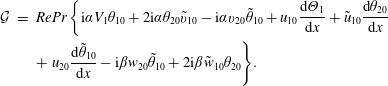 $$\begin{eqnarray}\displaystyle {\mathcal{G}} & = & \displaystyle RePr\left\{\text{i}\unicode[STIX]{x1D6FC}V_{1}\unicode[STIX]{x1D703}_{10}+2\text{i}\unicode[STIX]{x1D6FC}\unicode[STIX]{x1D703}_{20}\tilde{v}_{10}-\text{i}\unicode[STIX]{x1D6FC}v_{20}\tilde{\unicode[STIX]{x1D703}}_{10}+u_{10}\frac{\text{d}\unicode[STIX]{x1D6E9}_{1}}{\text{d}x}+\tilde{u} _{10}\frac{\text{d}\unicode[STIX]{x1D703}_{20}}{\text{d}x}\right.\nonumber\\ \displaystyle & & \displaystyle +\left.u_{20}\frac{\text{d}\tilde{\unicode[STIX]{x1D703}}_{10}}{\text{d}x}-\text{i}\unicode[STIX]{x1D6FD}w_{20}\tilde{\unicode[STIX]{x1D703}}_{10}+2\text{i}\unicode[STIX]{x1D6FD}\tilde{w}_{10}\unicode[STIX]{x1D703}_{20}\right\}\!.\end{eqnarray}$$
C.3 Linear adjoint equations
The solution of the adjoint system of linear instability equations (C 1)–(C 5) is needed to obtain the Landau constant. The definition of the adjoint operator is given as (Khandelwal & Bera Reference Khandelwal and Bera2015)
 $$\begin{eqnarray}\displaystyle \langle LX,X^{\ast }\rangle =\langle X,L^{\ast }X^{\ast }\rangle , & & \displaystyle\end{eqnarray}$$
where
 $X^{\ast }=[u^{\ast },v^{\ast },w^{\ast },\unicode[STIX]{x1D703}^{\ast },p^{\ast }]$
is the adjoint eigenfunction,
 $L=[\mathscr{L}_{o},\mathscr{L}_{x},\mathscr{L}_{y},\mathscr{L}_{z},\mathscr{L}]$
is the linear stability operator and
 $L^{\ast }=[\mathscr{L}_{o}^{\ast },\mathscr{L}_{x}^{\ast },\mathscr{L}_{y}^{\ast },\mathscr{L}_{z}^{\ast },\mathscr{L}^{\ast }]$
is the corresponding adjoint operator. The inner product in this definition is the standard inner product given as
 $$\begin{eqnarray}\displaystyle \langle Y(x),Z(x)\rangle =\int _{-1}^{1}Y^{\ast }(x)Z(x)\,\text{d}x=\int _{-1}^{1}\mathop{\sum }_{i=1}^{5}(y_{i}^{\ast }(x)z_{i}(x)\,\text{d}x, & & \displaystyle\end{eqnarray}$$
where the superscript
 $\ast$
denotes the adjoint eigenfunction. The corresponding adjoint equations of the linear stability equations (C 1)–(C 5) are given as
 $$\begin{eqnarray}\displaystyle \mathscr{L}_{o}^{\ast }(\unicode[STIX]{x1D6FC},\unicode[STIX]{x1D6FD},u^{\ast },v^{\ast },w^{\ast })=\frac{\text{d}u^{\ast }}{\text{d}x}-\text{i}\unicode[STIX]{x1D6FC}v^{\ast }-\text{i}\unicode[STIX]{x1D6FD}w^{\ast }=0, & & \displaystyle\end{eqnarray}$$
 $$\begin{eqnarray}\displaystyle & & \displaystyle \mathscr{L}_{x}^{\ast }(\unicode[STIX]{x1D6FC},\unicode[STIX]{x1D6FD},c,u^{\ast },v^{\ast },p^{\ast },\unicode[STIX]{x1D703}^{\ast },V_{0},\unicode[STIX]{x1D6E9}_{0},Da,F,Re)=\text{i}\unicode[STIX]{x1D6FC}Re\frac{1}{\unicode[STIX]{x1D700}}\left(\frac{1}{\unicode[STIX]{x1D700}}V_{0}-c\right)u^{\ast }+\frac{Re}{\unicode[STIX]{x1D700}^{2}}\frac{\text{d}V_{0}}{\text{d}x}v^{\ast }\nonumber\\ \displaystyle & & \displaystyle -\,\unicode[STIX]{x1D706}\left(\frac{\text{d}^{2}u^{\ast }}{\text{d}x^{2}}-(\unicode[STIX]{x1D6FC}^{2}+\unicode[STIX]{x1D6FD}^{2})u^{\ast }\right)-\frac{\text{d}p^{\ast }}{\text{d}x}+\frac{1}{Da}u^{\ast }+F^{\prime }|V_{0}|u^{\ast }-PrRe\frac{\text{d}\unicode[STIX]{x1D6E9}_{0}}{\text{d}x}\unicode[STIX]{x1D703}^{\ast }=0.\end{eqnarray}$$
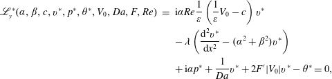 $$\begin{eqnarray}\displaystyle \mathscr{L}_{y}^{\ast }(\unicode[STIX]{x1D6FC},\unicode[STIX]{x1D6FD},c,v^{\ast },p^{\ast },\unicode[STIX]{x1D703}^{\ast },V_{0},Da,F,Re) & = & \displaystyle \text{i}\unicode[STIX]{x1D6FC}Re\frac{1}{\unicode[STIX]{x1D700}}\left(\frac{1}{\unicode[STIX]{x1D700}}V_{0}-c\right)v^{\ast }\nonumber\\ \displaystyle & & \displaystyle -\,\unicode[STIX]{x1D706}\left(\frac{\text{d}^{2}v^{\ast }}{\text{d}x^{2}}-(\unicode[STIX]{x1D6FC}^{2}+\unicode[STIX]{x1D6FD}^{2})v^{\ast }\right)\nonumber\\ \displaystyle & & \displaystyle +\,\text{i}\unicode[STIX]{x1D6FC}p^{\ast }+\frac{1}{Da}v^{\ast }+2F^{\prime }|V_{0}|v^{\ast }-\unicode[STIX]{x1D703}^{\ast }=0,\end{eqnarray}$$
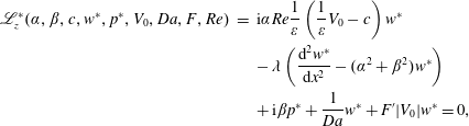 $$\begin{eqnarray}\displaystyle \mathscr{L}_{z}^{\ast }(\unicode[STIX]{x1D6FC},\unicode[STIX]{x1D6FD},c,w^{\ast },p^{\ast },V_{0},Da,F,Re) & = & \displaystyle \text{i}\unicode[STIX]{x1D6FC}Re\frac{1}{\unicode[STIX]{x1D700}}\left(\frac{1}{\unicode[STIX]{x1D700}}V_{0}-c\right)w^{\ast }\nonumber\\ \displaystyle & & \displaystyle -\,\unicode[STIX]{x1D706}\left(\frac{\text{d}^{2}w^{\ast }}{\text{d}x^{2}}-(\unicode[STIX]{x1D6FC}^{2}+\unicode[STIX]{x1D6FD}^{2})w^{\ast }\right)\nonumber\\ \displaystyle & & \displaystyle +\,\text{i}\unicode[STIX]{x1D6FD}p^{\ast }+\frac{1}{Da}w^{\ast }+F^{\prime }|V_{0}|w^{\ast }=0,\end{eqnarray}$$
 $$\begin{eqnarray}\displaystyle \mathscr{L}^{\ast }(\unicode[STIX]{x1D6FC},\unicode[STIX]{x1D6FD},c,v^{\ast },\unicode[STIX]{x1D703}^{\ast },V_{0},Ra) & = & \displaystyle -\text{i}\unicode[STIX]{x1D6FC}PrRe(V_{0}-\unicode[STIX]{x1D70E}c)\unicode[STIX]{x1D703}^{\ast }+\left(\frac{\text{d}^{2}\unicode[STIX]{x1D703}^{\ast }}{\text{d}x^{2}}-(\unicode[STIX]{x1D6FC}^{2}+\unicode[STIX]{x1D6FD}^{2})\unicode[STIX]{x1D703}^{\ast }\right)\nonumber\\ \displaystyle & & \displaystyle -\,Ra\,v^{\ast }=0.\end{eqnarray}$$
The above equations are solved by eliminating the pressure terms along with the no-slip and impermeability conditions of the velocity and zero temperature perturbation on the walls. The corresponding boundary conditions for adjoint system are
 $$\begin{eqnarray}\displaystyle u^{\ast }=v^{\ast }=w^{\ast }=\unicode[STIX]{x1D703}^{\ast }=0\quad \text{at}~x=\pm 1. & & \displaystyle\end{eqnarray}$$
These adjoint eigenfunctions are also normalized to satisfy the equation
 $$\begin{eqnarray}\displaystyle \int _{-1}^{1}\left[\frac{1}{\unicode[STIX]{x1D700}}(\hat{u} u^{\ast }+\hat{v}v^{\ast }+{\hat{w}}w^{\ast })-Pr\hat{\unicode[STIX]{x1D703}}\unicode[STIX]{x1D703}^{\ast }\right]\text{d}x=1. & & \displaystyle\end{eqnarray}$$