4.1. Vary ${{Le_\tau }}$; other parameters are fixed

The steady-state profiles for a shallow chamber are dependent on ${{Le_\tau }}$, ${{H_\tau }}$ and ${{S_\tau }}$; however, in Hillesdon & Pedley (Reference Hillesdon and Pedley1996), these profiles are independent of $\delta _\textrm {HP}$ and vary only with $\gamma _\textrm {HP}\beta _\textrm {HP}$. It is also important to recall that they considered the vertical axis of the shallow chamber as $z=1$ at bottom and $z=0$ at the top, whereas we have taken the axis to be the vertical direction opposite to it, i.e. $z=0$ at the bottom and $z=1$ at the top boundary. We have changed the axes orientation of the model of Hillesdon & Pedley (Reference Hillesdon and Pedley1996) and presented their results in comparison with ours in figure 2. Since the steady-state solutions of cell and oxygen concentrations in Hillesdon & Pedley (Reference Hillesdon and Pedley1996) are independent of $\delta _\textrm {HP}$, we have compared our steady-state results for ${{Le_\tau }}=1$ and also varied the value of ${{Le_\tau }}=5$ to study the impact of the diffusivity variations. The results for a variety of shallow chamber examples have been presented, in which they covered the whole steady-state density profiles ranging from ${{S_\tau }}{{H_\tau }}/{{Le_\tau }}\sim \gamma _\textrm {HP}\beta _\textrm {HP}=0.8$ (nearly uniform) to ${{S_\tau }}{{H_\tau }}/{{Le_\tau }}\sim \gamma _\textrm {HP}\beta _\textrm {HP}=300$ (highly dense at the top). It can be observed from the comparison that the concentration levels of both cells and oxygen are equally distributed. However, the variation of ${{Le_\tau }}$ shows that the movement of the cells becomes much faster as the diffusivity of oxygen increases. Figures 2(a) and 2(b) show the steady-state cell and oxygen concentration profiles, respectively, at the uniform stage, and figures 2(c) and 2(d) show the profiles at the top of the shallow chamber, where the cell concentration starts getting denser (i.e. at the top boundary). Cell mobility in the present study is comparatively rapid but in a less non-scattered manner compared with that in the study by Hillesdon & Pedley (Reference Hillesdon and Pedley1996). In fact, the cell concentration profile is found to be quite close to the oxygen distribution profile. It should be noted that the impact of the surface tension will be seen in the perturbed cell and oxygen concentration profiles in the linear stability analysis since the surface tension is non-zero at the free surface.

Figure 2.

Steady-state cell and oxygen concentration profiles of Hillesdon & Pedley (Reference Hillesdon and Pedley1996) are plotted to make a comparison with those of the present study. The parameter values of $\gamma _\textrm {HP}\sim {{S_\tau }}=1$ and $\beta _\textrm {HP}\sim {{H_\tau }}=0.8$ in (a,b); and $\gamma _\textrm {HP}\sim {{S_\tau }}=5$ and $\beta _\textrm {HP}\sim {{H_\tau }}=60$ in (c,d), are taken into account.

In § 2, we have mentioned that the five dimensionless parameters ${{Le_\tau }}$, ${{H_\tau }}$, ${{S_\tau }}$, ${{Pr_\tau }}$ and ${{Ra_\tau }}$ are slightly different from those Hillesdon & Pedley (Reference Hillesdon and Pedley1996) referred to. A few estimated parametric values from the linear stability analysis conducted in the present study are compared with the published results of Hillesdon & Pedley (Reference Hillesdon and Pedley1996) in table 1. The differences are apparent because the present study involves the values of ${{Fr_\tau }}$ and ${{Ca_\tau }}$. Among the ten sets of results, only six have been compared with the results of Hillesdon & Pedley (Reference Hillesdon and Pedley1996), which can be seen in table 1; the neutral stability curves ${{Ra_\tau }}(k)$ are plotted in figure 4 and figure 7 shows the variation of other parameters. The estimated results of ${{Ra_\tau }}_c$ and the corresponding values of $k_c$ vs ${{S_\tau }}{{H_\tau }}$ with the varying values of other parameters are visualized in figure 3. Some interesting points can be observed in these computed results of ${{Ra_\tau }}_c$ and $k_c$. Firstly, we can see in figure 7(c) that the neutral curves for the different values of ${{Le_\tau }}$ (fixed ${{S_\tau }}{{H_\tau }}=1$) diverge initially and then gradually converge as the wavenumber increases. Conversely, in the study by Hillesdon & Pedley (Reference Hillesdon and Pedley1996), neutral curves diverged for different values of $\delta _{HP}$ as the wavenumber increased (see figure 5 in Hillesdon & Pedley Reference Hillesdon and Pedley1996). Secondly, the computed value of ${{Ra_\tau }}$ for a given $k$ is larger for ${{Le_\tau }}=10$ than for ${{Le_\tau }}=1$, i.e. as ${{Le_\tau }}$ increases, the system stabilizes. The same trend can be seen in the work of Hillesdon & Pedley (Reference Hillesdon and Pedley1996). Interestingly, the computed values of ${{Ra_\tau }}_c$ and $k_c$ for the present study in case sets 2 and 8 are the same. The interpretation of these results is not straightforward. The increment in the value of ${{Le_\tau }}$ can be expressed either as an increase in $D_O$ with fixed $D_b$ or as a decrease in $D_b$ with fixed $D_O$, and the decreasing value of ${{Le_\tau }}$ can be expressed vice versa. A difference can be seen between the present study and that of Hillesdon & Pedley (Reference Hillesdon and Pedley1996) for the case sets in table 1 and figure 4. In our study, the neutral stability curve for ${{Le_\tau }}=1$, ${{S_\tau }}=1$ and ${{H_\tau }}=1$ slowly diverges initially and then gradually stabilizes as $k$ increases, whereas for Hillesdon & Pedley (Reference Hillesdon and Pedley1996), it diverged for any given $k$.

Figure 3.

(a) Critical values of Rayleigh number, ${{Ra_\tau }}_c$, and (b) the corresponding values of the critical wavenumber are computed for varying ${{Le_\tau }}$; (c) the variation of $\varepsilon$ and (d) Froude numbers ${{Fr_\tau }}$ are shown for fixed values of ${{Le_\tau }}=1$ and ${{Pr_\tau }}=7700$. The minimum value in the curve is ${{{S_\tau }}{{H_\tau }}}/{{{Le_\tau }}}\approx 1.936$.

Figure 4.

Comparison of the neutral stability curve of the present study (a) with the result of Hillesdon & Pedley (Reference Hillesdon and Pedley1996) (b) for shallow chamber.

Table 1.

The estimated values of ${{Ra_\tau }}_c$ and $k_c$ for the shallow chamber case are presented where -HP and -Present represent the values of Hillesdon & Pedley (Reference Hillesdon and Pedley1996) and the present work, respectively.

It can be visualized from the table 1 that, with the increasing value of ${{Le_\tau }}$, a plane free surface density gradient occurs for larger values of ${{S_\tau }}{{H_\tau }}$. However, the value of ${{Ra_\tau }}_c$ first drops as ${{S_\tau }}{{H_\tau }}$ is increased and then rises again. Besides, $k_c$ has a maximum value, although the minimum values of $k_c$ and ${{Ra_\tau }}_c$ are not obtained at the same value as ${{S_\tau }}{{H_\tau }}$. This behaviour is exhibited in figures 3(a) and 3(b), which show the critical Rayleigh number, ${{Ra_\tau }}_c$, and the corresponding value of $k_c$ being plotted against ${{S_\tau }}{{H_\tau }}$ for varying values of ${{Le_\tau }}$. From the figure, we can see that, for each value of ${{Le_\tau }}$, the minimum value of ${{Ra_\tau }}_c$ is found when ${{S_\tau }}{{H_\tau }}/{{Le_\tau }}\approx 1.936$. From this detection, it is now clear that ${{Ra_\tau }}$ might not be suitable for measuring the ratio between the buoyancy force that leads to bioconvection and the viscous force that intercepts it.

The frequency of oscillation vs ${{S_\tau }}{{H_\tau }}$ is plotted with the variation of ${{Le_\tau }}$ in figure 8(a). It can be observed from the figure that the growth rate is not affected by the variation of ${{Le_\tau }}$. However, in the growth rate, the curve shift towards higher ${{S_\tau }}{{H_\tau }}$ becomes noticeable as the value of the Lewis number increases. This behavioural change is due to the increasing value of ${{Le_\tau }}$. Hence, the cell diffusivity is extremely less than oxygen, i.e. a smaller cell concentration at the interface leads to greater discontinuity (the system becomes unstable). Besides, the presence of ${{Fr_\tau }}$ aids in increasing the cell concentration with increasing ${{Le_\tau }}$.

The characteristics of the perturbed cell and oxygen concentrations and velocity profiles are illustrated in figures 10(a), 11(a) and 12(a), respectively, corresponding to the values of ${{Ra_\tau }}_c$ and $k_c$ for a shallow chamber with the variation of ${{Le_\tau }}$. It is clear from figure 10(a) that, as the value of ${{Le_\tau }}$ increases, the concentration of cells decreases at the air–water interface, and their movement towards the free surface is steady. With decreasing ${{Le_\tau }}$, the cells get denser, and the cells’ movement towards the free surface is more rapid. The aggregation of cells is mostly found just below the layer of free surface. This result justifies that, when the oxygen diffusion is higher, then the cell diffusivity is small or constant, and so are the critical values of ${{Ra_\tau }}_c$ and $k_c$, which start to fall with the increase of ${{Le_\tau }}$. As ${{Le_\tau }}$ increases, the diffusivity of oxygen also increases, and this statement is supported by the oxygen concentration profiles presented in figure 11(a) for the variation of ${{Le_\tau }}=0.5, 1, 5$. Figure 12(a) shows the characteristics of the perturbed fluid velocity profiles for a shallow chamber corresponding to the values of ${{Ra_\tau }}_c$ and $k_c$. The intensity of the wave profile for ${{Le_\tau }}=0.5$ is much higher than that for the case with the increasing value of ${{Le_\tau }}$. Eventually, an increase in the diffusivity of oxygen makes the system unstable, and vice versa, as ${{Le_\tau }}$ decreases. The flow motion in the chemotaxis system is interrupted at the onset of convection, however, it stabilizes after reaching the free surface.

Thus far, the results have been compared when there is variation in ${{Le_\tau }}$ and the other physical parameters are fixed at $\varepsilon =0.1$, ${{S_\tau }}{{H_\tau }}=1$, ${{Pr_\tau }}=7700$, ${{Fr_\tau }}=0.001$ and ${{Ca_\tau }}=0.01$. In the next stage, the impact of the Froude number is discussed by varying the ${{Fr_\tau }}$ values to $0.001, 0.003$ and $0.006$ and fixing the other parameters at ${{Le_\tau }}=1$, $\varepsilon =0.1$, ${{S_\tau }}{{H_\tau }}=1$, ${{Pr_\tau }}=7700$ and ${{Ca_\tau }}=0.01$. It is noteworthy that the results of figures 10, 11 and 12, are plotted from the eigenvalue problem.

4.2. Vary ${{Fr_\tau }}$; other parameters are fixed

The values of ${{Ra_\tau }}_c$ and $k_c$ have been computed by varying the Froude number and presented in table 1. It can be observed from the parameter sets two, nine and ten that for ${{Fr_\tau }}=0.001$, $0.003$ and $0.006$, the computed ${{Ra_\tau }}_c$ values are $811.183$, $1028.42$ and $1761.58$, respectively, whereas $k_c$ gives the same value of $34.4$ for different ${{Fr_\tau }}$ (here, ${{S_\tau }}{{H_\tau }}=1$ and ${{Le_\tau }}=1$). This situation is also illustrated in figure 3(d), where $k_c$ vs ${{S_\tau }}{{H_\tau }}$ is plotted for the varying values of ${{Fr_\tau }}$. Notably, under the variation of ${{Fr_\tau }}$, $k_c$ shows the same critical value at the minimum value of ${{S_\tau }}{{H_\tau }}$. This implies that the wavenumber is not influenced by the change in ${{S_\tau }}{{H_\tau }}$ though the initial jump found is due to the change in ${{Fr_\tau }}$. As the value of the Froude number increases, the wavenumber reaches its maximum value in the uniform stage of the system. Otherwise, the wavenumber is constant throughout the system. In figure 7(d), neutral stability curves are shown under the variation of ${{Fr_\tau }}$. Due to the presence of ${{Fr_\tau }}$, the flow at the free surface accelerates under the action of gravity. As the value of ${{Fr_\tau }}$ increases, the flow accelerates even further for ${{Fr_\tau }}=0.006$ compared with those at other values of Froude number. Therefore, initially, the system seems to be destabilized, however, it stabilizes as the wavenumber increases. However, if we look at the result of the oscillation of frequency curves in figure 8(c), it shows a minute deflation in the growth rate as ${{Fr_\tau }}$ increases. However, quite a big shift is noticed in the growth rate. The frequency of oscillations vs ${{S_\tau }}{{H_\tau }}$ is illustrated in figure 8(c) for the variation of ${{Fr_\tau }}$. In other words, a decrease in the frequency of oscillations causes the system to become stabilized.

The real parts of the perturbed cell and oxygen concentrations and velocity profiles are plotted by varying ${{Fr_\tau }}=0.001$, $0.003,$ and $0.006$ in figures 10(f), 11(f) and 12(e), respectively, corresponding to the values of ${{Ra_\tau }}_c$ and $k_c$. Both the cell and oxygen concentration profiles show a subtle effect on the upper surface rather than the bottom surface of the chemotaxis system. Although the differences are very small, the cell concentration profile decreases as ${{Fr_\tau }}$ increases with a steady motion and gradually reaches towards the free surface. The same situation is also seen for the perturbed oxygen concentration profiles. The significant effect of ${{Fr_\tau }}$ is visible at the perturbed fluid velocity profiles, where on increasing the value of ${{Fr_\tau }}$, the velocity of the fluid becomes steady at the free surface. It stabilizes the motion of the fluid close to the free surface, where the concentrations of both cells and oxygen are balanced. Whereas the comparison between the profiles of $N_r$, $C_r$ and $W_r$ slightly differs for the higher value of ${{Fr_\tau }}$.

4.3. Vary ${{Ca_\tau }}$; other parameters are fixed

The frequency of oscillations vs ${{S_\tau }}{{H_\tau }}$ is illustrated in figure 8(b) for the variation of ${{Ca_\tau }}$. The increasing value of ${{Ca_\tau }}$ shows an inflation in the growth rate along with a small shift, leading the system to be stable. The curves widen due to the increasing value of ${{S_\tau }}{{H_\tau }}$ as ${{Ca_\tau }}$ increases, and the peak value falls, giving stability to the system at the free surface in the shallow chamber case. The frequency of oscillation, $\omega$, vs $k$ is plotted in figure 9(b) for the variation of ${{Ca_\tau }}$. The same scenario can be seen here for the frequency of oscillations where the curves get wider and the peaks rise with the increasing wavenumber, however, this occurs for the decreasing value of ${{Ca_\tau }}$. A slight tilt in the front of the curves can be seen for the decreasing value of ${{Ca_\tau }}$. This explains that the surface tension is tenacious enough to hold the exalted wave profile.

The real parts of the perturbed cell and oxygen concentrations, and velocity profiles are plotted by varying ${{Ca_\tau }}=0.005$, $0.01,$ and $0.05$ in figures 10(e), 11(e) and 12(d), respectively, which are corresponding to the values of ${{Ra_\tau }}_c$ and $k_c$. A similar scenario can be seen in figures 10(f) and 11(f) for the variation of ${{Fr_\tau }}$. Note that in figures 10(e) and 11(e) we mentioned the perturbed cell and oxygen concentrations for varying values of ${{Ca_\tau }}$. Figure 12(d) shows the different characteristics of the perturbed fluid velocity profile $W_r$ in a shallow chamber with the variation of ${{Ca_\tau }}$. It is clear from the figure that the velocity profile $W_r$ increases with an increasing value of ${{Ca_\tau }}$. The comparison between the profiles of $W_r$ (the perturbed fluid velocity), $N_r$ (the perturbed cell concentration) and $C_r$ (the perturbed oxygen concentration) detects a random movement of cells in the system as lack in oxygen makes the system unstable. The chemotaxis system stabilizes as the surface tension increases at the free surface. However, at the onset of convection, the system shows a destabilizing effect. The concentrations of cells and oxygen increase near the free surface, and almost all cells are accumulated near the stable free surface.

4.4. Vary ${{S_\tau }}{{H_\tau }}$; other parameters are fixed

In table 1, the estimated values of ${{Ra_\tau }}_c$ and $k_c$ for shallow chamber are given for the variation of ${{S_\tau }}{{H_\tau }}$ and ${{Le_\tau }}$. These values of ${{Ra_\tau }}_c$ and $k_c$ are compared with those of Hillesdon & Pedley (Reference Hillesdon and Pedley1996) though the comparison by varying ${{Le_\tau }}$ has been discussed in the previous section. In linear stability analysis, we have fixed the value of ${{Le_\tau }}$, and independently varied the values of ${{S_\tau }}$ and ${{H_\tau }}$. These variations can be seen in figures 5 and 6 are discussed in detail later in this section. In table 1, data sets 1–7, we have fixed the values of ${{Le_\tau }}=1$ and ${{S_\tau }}=1$, and varied ${{H_\tau }}$ from $0.05$ to $100$. It can be observed that, in the uniform stage of the system (${{H_\tau }}=0.05$), the critical Rayleigh number is estimated to take the highest value and similarly for the critical wavenumber. It can be seen that, as the value of ${{H_\tau }}$ increases, the value of the critical Rayleigh number drops. The minimum value of the critical Rayleigh number is found when ${{H_\tau }}=10$. Then, the value of critical Rayleigh number starts to rise again as the value of ${{H_\tau }}$ starts increasing. When $k\to 0$, the analytical approximation is ${{Ra_\tau }}\to {1440{{Le_\tau }}}/{7{{S_\tau }}{{H_\tau }}}=4114.29$. The critical values of the Rayleigh number and wavenumber are ${{Ra_\tau }}_c=15234.24$ and $k_c=154.4$. It can be anticipated that our numerically predicted first pattern would be experimentally seen when ${{Ra_\tau }}$ is slowly reduced to ${{Ra_\tau }}_c$. In general, the most unstable disturbance occurred for ${{Ra_\tau }}>{{Ra_\tau }}_c$, which has a different wavelength. The approximate value of a dimensionless wavelength $\lambda _c=2{\rm \pi} /k_c$ can be calculated from the value of the critical wavenumber $k_c$. It would be interesting to conduct an experiment using the present model to verify these estimated results and predictions.

Figure 5.

(a) The curves ${{Ra_\tau }}$ and (b) $\omega _i$ corresponding to varying values of ${{S_\tau }}$ at fixed values of ${{Le_\tau }}=1$, $\varepsilon =0.1$, ${{H_\tau }}=10$, ${{Pr_\tau }}=7700$, ${{Fr_\tau }}=0.001$ and ${{Ca_\tau }}=0.01$.

Figure 6.

The curves ${{Ra_\tau }}$ and (b) $\omega _i$ corresponding to varying values of ${{H_\tau }}$ at fixed values of ${{Le_\tau }}=1$, $\varepsilon =0.1$, ${{S_\tau }}=5$, ${{Pr_\tau }}=7700$, ${{Fr_\tau }}=0.001$ and ${{Ca_\tau }}=0.01$.

In figures 5 and 6, the neutral stability and growth rate, respectively, are plotted with the variations of ${{S_\tau }}$ and ${{H_\tau }}$ separately. In figure 5, ${{S_\tau }}$ is varied from $1$ to $5$, and ${{H_\tau }}$ is varied from $10$ to $50$ in figure 6. Interestingly, all the neutral stability curves in figures 5(a) and 6(a) for the variation of ${{S_\tau }}$ and ${{H_\tau }}$, respectively, intersect at a point when ${{Ra_\tau }}=205.71$. Further, all the curves of the growth rate in figures 5(b) and 6(b) for the variation of ${{S_\tau }}$ and ${{H_\tau }}$, respectively, have the cutoff wavenumber $k=12.8$. In figures 5(a) and 6(a), all the neutral stability curves for different values ${{S_\tau }}$ and ${{H_\tau }}$ converge as the wavenumber increases. In fact, the value of ${{Ra_\tau }}$, for a given $k$, is larger, for ${{S_\tau }}=5$ and ${{H_\tau }}=10$, than for the other lower varying values of ${{S_\tau }}$ and ${{H_\tau }}$. It is implied that an increase in the values of ${{S_\tau }}$ and ${{H_\tau }}$ is evidently stabilizing. The qualitative behaviour in each case is the same, as the wavenumber $k$ increases, the Rayleigh number ${{Ra_\tau }}$ decreases steadily to its minimum value. The variation in ${{H_\tau }}$ shows that the motion of fluid at the critical Rayleigh number consists of convective cells. Thus, the cells initiated in the upper unstable layer penetrate through the stable layer and reach towards the bottom layer. The convection starts in this situation, and soon, the whole chamber becomes involved in this motion. This initial motion, observed experimentally, has a wavenumber, and this wavenumber is presumed to be equal to the most unstable wavenumber corresponding to the value of ${{Ra_\tau }}$. Similarly, the growth rates in figures 5(b) and 6(b) show higher inflation for large values of ${{S_\tau }}$ and ${{H_\tau }}$, i.e. increase in ${{S_\tau }}$ and ${{H_\tau }}$ is apparently stabilizing. The growth rate corresponding to a particular wavenumber is greatest in ${{S_\tau }}=5$ and ${{H_\tau }}=50$, for $k>4$.

In figures 10(d) and 10(c), 11(d) and 11(c) and 12(c), the characteristics of the perturbed cell and oxygen concentrations, and the fluid velocity profiles, respectively, are presented with respect to the length of the shallow chamber corresponding to the values of ${{Ra_\tau }}_c$ and $k_c$. In figures 10(d) and 10(c), ${{H_\tau }}$ is varied from $1$ to $5$, respectively, whereas ${{S_\tau }}$ is fixed at $1$. The concentration of cells for ${{H_\tau }}=1$ is less at the bottom of the chamber and increases near the free surface (see figure 10d). Moreover, in figure 10(c), the concentration of cells for ${{H_\tau }}=5$ is even lower than that for ${{H_\tau }}=1$, and, similarly, it increases near the free surface. In figures 10(d) and 10(c), the concentration of oxygen gradually increases for ${{H_\tau }}=1$ as moving towards the free surface. Moreover, as expected, the most apparent difference is seen in the $C_r$ distribution profile for ${{H_\tau }}=5$. Although, both cell and oxygen zero-flux conditions are satisfied at $z=0$. The distribution of $C$ is mostly interrupted within the system due to the excessive consumption of the oxygen. The fluid velocity profile $W_r$ increases with the increasing value of ${{H_\tau }}$ (see in figure 12c). The difference in the velocity profiles becomes more noticeable as the value of ${{H_\tau }}$ increases.

4.5. Variation of $\varepsilon$ and ${{Pr_\tau }}$

The length of the shallow chamber has also been varied to investigate the nature of the stability and the impact of $\varepsilon$ on the present system. The variation of $\varepsilon$ presented in table 1 shows that the estimated values of ${{Ra_\tau }}_c$ remained unchanged for different $\varepsilon$ although the estimated values of $k_c$ increased with decreasing $\varepsilon$. It can be said that the number of waves increases as the length of the chamber increases. These results are illustrated in figure 3(c) where one can clearly visualize that the critical wavenumber increases with the decreasing value of $\varepsilon$ and is not influenced by the change in ${{S_\tau }}{{H_\tau }}$. This statement can also be verified through figure 7(b), in which the neutral stability curves show a stabilizing effect in the increasing cutoff wavenumber when the length of the chamber increases although ${{Ra_\tau }}$ is not influenced by the change. The impact of the chamber length can also be seen in the frequency of oscillations, where the growth rate is illustrated against the wavenumber in figure 9(a).

Figure 7.

Neutral stability curves presented with the variation of ${{H_\tau }}, {{S_\tau }}$ in (a) (fixed ${{Le_\tau }}=1$, $\varepsilon =0.1$, ${{Pr_\tau }}=7700$, ${{Ca_\tau }}=0.01$, ${{Fr_\tau }}=0.001$), $\varepsilon$ in (b) (fixed ${{Le_\tau }}=1$, ${{S_\tau }},{{H_\tau }}=1$, ${{Pr_\tau }}=7700$, ${{Ca_\tau }}=0.01$, ${{Fr_\tau }}=0.001$), ${{Le_\tau }}$ in (c) (fixed $\varepsilon =0.1$, ${{S_\tau }},{{H_\tau }}=1$, ${{Pr_\tau }}=7700$, ${{Ca_\tau }}=0.01$, ${{Fr_\tau }}=0.001$), ${{Fr_\tau }}$ in (d) (fixed ${{Le_\tau }}=1$, $\varepsilon =0.1$, ${{S_\tau }},{{H_\tau }}=1$, ${{Pr_\tau }}=7700$, ${{Ca_\tau }}=0.01$) and ${{Pr_\tau }}$ in (e) (fixed ${{Le_\tau }}=1$, $\varepsilon =0.1$, ${{S_\tau }},{{H_\tau }}=1$, ${{Ca_\tau }}=0.01$, ${{Fr_\tau }}=0.001$).

Figure 8.

The curves of $\omega$ are presented at the critical ${{Ra_\tau }}$ with the variation of ${{Le_\tau }}$ in (a) (fixed ${{Ca_\tau }}=0.01$, ${{Fr_\tau }}=0.001$), ${{Ca_\tau }}$ in (fixed ${{Le_\tau }}=1$, ${{Fr_\tau }}=0.001$) (b) and ${{Fr_\tau }}$ in (fixed ${{Le_\tau }}=1$, ${{Ca_\tau }}=0.01$) (c).

Figure 9.

The curves of $\omega$ are presented at the critical ${{Ra_\tau }}$ with the variation of $\varepsilon$ in (a) (fixed ${{Ca_\tau }}=0.01$) and ${{Ca_\tau }}$ in (b) (fixed $\varepsilon =0.1$). Other parameters are fixed at ${{Le_\tau }}=1$, ${{S_\tau }}=1$, ${{H_\tau }}=1$, ${{Fr_\tau }}=0.001$ and ${{Pr_\tau }}=7700$.

In figures 10(b), 11(b) and 12(b), the characteristics of the perturbed cell and oxygen concentrations, and fluid velocity profiles, respectively, are presented with the variation in the length of the shallow chamber corresponding to the values of ${{Ra_\tau }}_c$ and $k_c$. It can be observed in figure 10(b) that the cell concentrations at the free surface for a small chamber are lower than in the long chamber in comparison with those at the bottom of the shallow chamber. Therefore, it can be stated that the cell concentration will increase with an increasing length of the chamber. However, the oxygen concentration profiles in figure 11(b) show that the oxygen concentration level will be identical at the free surface for differently sized chambers although at the bottom of the chamber, the oxygen concentration level will increase/decrease as the length of the chamber decreases/increases. Figure 12(b) shows that the variation in the length of the chamber has a significant impact on the velocity of the wave profiles. As the length of the chamber increases, we can observe steady velocity profiles, whereas the velocity of the wave profile increases as the length of the chamber decreases.

Figure 10.

Different characteristics of the perturbed cell concentration profiles $N_r$ are presented corresponding to the values of ${{Ra_\tau }}_c$ and $k_c$ for shallow chamber with the variation of ${{Le_\tau }}$ in (a) (fixed $\varepsilon =0.1$, ${{S_\tau }}, {{H_\tau }}=1$, ${{Pr_\tau }}=7700$, ${{Ca_\tau }}=0.01$ and ${{Fr_\tau }}=0.001$); $\varepsilon$ in (b) (fixed ${{Le_\tau }}=1$, ${{S_\tau }},{{H_\tau }}=1$, ${{Pr_\tau }}=7700$, ${{Ca_\tau }}=0.01$ and ${{Fr_\tau }}=0.001$); ${{Ca_\tau }}$ in (e) (fixed $\varepsilon =0.1$, ${{Le_\tau }}=1$, ${{S_\tau }},{{H_\tau }}=1$, ${{Pr_\tau }}=7700$ and ${{Fr_\tau }}=0.001$); ${{Fr_\tau }}$ in (f) (fixed $\varepsilon =0.1$, ${{Le_\tau }}=1$, ${{S_\tau }},{{H_\tau }}=1$, ${{Pr_\tau }}=7700$ and ${{Ca_\tau }}=0.01$). Panels (c,d) show the profiles for ${{S_\tau }},{{H_\tau }}=1$ and ${{S_\tau }},{{H_\tau }}=5$ and other parameters are fixed at $\varepsilon =0.1$, ${{Le_\tau }}=1$, ${{Pr_\tau }}=7700$, ${{Ca_\tau }}=0.01$ and ${{Fr_\tau }}=0.001$.

Figure 11.

Different characteristics of the perturbed oxygen concentration profiles $C_r$ are presented corresponding to the values of ${{Ra_\tau }}_c$ and $k_c$ for shallow chamber with the variation of ${{Le_\tau }}$ in (a) (fixed $\varepsilon =0.1$, ${{S_\tau }},{{H_\tau }}=1$, ${{Pr_\tau }}=7700$, ${{Ca_\tau }}=0.01$ and ${{Fr_\tau }}=0.001$); $\varepsilon$ in (b) (fixed ${{Le_\tau }}=1$, ${{S_\tau }},{{H_\tau }}=1$, ${{Pr_\tau }}=7700$, ${{Ca_\tau }}=0.01$ and ${{Fr_\tau }}=0.001$); ${{Ca_\tau }}$ in (e) (fixed $\varepsilon =0.1$, ${{Le_\tau }}=1$, ${{S_\tau }},{{H_\tau }}=1$, ${{Pr_\tau }}=7700$ and ${{Fr_\tau }}=0.001$); ${{Fr_\tau }}$ in (f) (fixed $\varepsilon =0.1$, ${{Le_\tau }}=1$, ${{S_\tau }},{{H_\tau }}=1$, ${{Pr_\tau }}=7700$ and ${{Ca_\tau }}=0.01$). Panels (c,d) show the profiles for ${{S_\tau }},{{H_\tau }}=1$ and ${{S_\tau }},{{H_\tau }}=5$ and other parameters are fixed at $\varepsilon =0.1$, ${{Le_\tau }}=1$, ${{Pr_\tau }}=7700$, ${{Ca_\tau }}=0.01$ and ${{Fr_\tau }}=0.001$.

Figure 12.

Different characteristics of the perturbed fluid velocity profiles $W_r$ are presented corresponding to the values of ${{Ra_\tau }}_c$ and $k_c$ for shallow chamber with the variation of ${{Le_\tau }}$ in (a) (fixed $\varepsilon =0.1$, ${{S_\tau }}, {{H_\tau }}=1$, ${{Pr_\tau }}=7700$, ${{Ca_\tau }}=0.01$ and ${{Fr_\tau }}=0.001$); $\varepsilon$ in (b) (fixed ${{Le_\tau }}=1$, ${{S_\tau }},{{H_\tau }}=1$, ${{Pr_\tau }}=7700$, ${{Ca_\tau }}=0.01$ and ${{Fr_\tau }}=0.001$); ${{S_\tau }},{{H_\tau }}$ in (c) (fixed $\varepsilon =0.1$, ${{Le_\tau }}=1$, ${{Pr_\tau }}=7700$, ${{Ca_\tau }}=0.01$ and ${{Fr_\tau }}=0.001$); ${{Ca_\tau }}$ in (d) (fixed $\varepsilon =0.1$, ${{Le_\tau }}=1$, ${{S_\tau }},{{H_\tau }}=1$, ${{Pr_\tau }}=7700$ and ${{Fr_\tau }}=0.001$); ${{Fr_\tau }}$ in (e) (fixed $\varepsilon =0.1$, ${{Le_\tau }}=1$, ${{S_\tau }},{{H_\tau }}=1$, ${{Pr_\tau }}=7700$ and ${{Ca_\tau }}=0.01$).

We have varied ${{Pr_\tau }}$ from $500\sim 7700$ to investigate the impact of the Prandtl number on the chemotaxis system, and this is shown in figure 7(e). It can be observed from the figure that the trend of the curves is similar for the variation of ${{Pr_\tau }}$. As ${{Pr_\tau }}$ increases, the value of ${{Ra_\tau }}$ increases along with the value of wavenumber. Here, ${{Pr_\tau }}$ is defined as the ratio of the fluid diffusivity to cell diffusivity, and the values are varied for $500\leqslant {{Pr_\tau }}\leqslant 7700$, i.e. the viscosity of the fluid is higher than the cell diffusivity, and this brings instability to the chemotaxis system. Since all the curves show a similar nature in the figure, so the highest value of ${{Pr_\tau }}({=}7700)$ is considered for the parametric study.

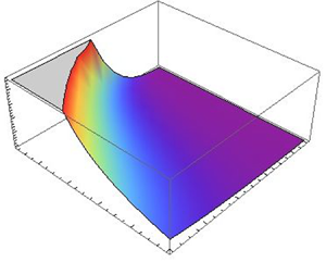
Since ${{Fr_\tau }}$ and ${{Ca_\tau }}$ are two important physical parameters in this system, we have varied both the parameters together as well as the other parameters such as ${{Le_\tau }}$ and $\varepsilon$ to study their influence on the stability of the chemotaxis system. The frequency of oscillations, $\omega$, vs ${{Fr_\tau }}$ and ${{Ca_\tau }}$ is plotted in figure 13. The figure shows that the peak of the frequency of the oscillation curve increases with a decreasing value of ${{Ca_\tau }}$, and the increase in the peak of the curve is also influenced by an increasing value of ${{Fr_\tau }}$. The curve exponentially increases with the increasing value of ${{Fr_\tau }}$. Based on the results in the figure, we can say that the surface tension force is strong enough to hold the peak of the wave, although increasing the value of ${{Fr_\tau }}$ enables the curve to take its peak value. Then, at a much lower value of ${{Ca_\tau }}$ and higher value of ${{Fr_\tau }}$, the frequency of the oscillation curve converges indicating the stabilization of the chemotaxis system.

Figure 13.

Frequency of oscillation, $\omega$, is plotted for the variations of ${{Ca_\tau }}$ and ${{Fr_\tau }}$ corresponding to the values of ${{Ra_\tau }}_c$ and $k_c$ for shallow chamber, and other parameters are fixed at $\varepsilon =0.1$, ${{Le_\tau }}=1$, ${{S_\tau }}=1$, ${{H_\tau }}=10$ and ${{Pr_\tau }}=7700$.

The critical Rayleigh number, ${{Ra_\tau }}_c$, vs ${{Le_\tau }}$ and ${{Fr_\tau }}$ is plotted in figure 14(a), and in figure 14(b), plotted against $\varepsilon$ and ${{Fr_\tau }}$. It can be seen in figure 14(a) that the value of ${{Ra_\tau }}$ drops initially when the value of ${{Le_\tau }}$ is smaller, however, then it diverges as the value of ${{Le_\tau }}$ increases. Here, it is worth mentioning that ${{Ra_\tau }}_c$ also depends on the parameters ${{S_\tau }}$ and ${{H_\tau }}$. The values of ${{S_\tau }}$ and ${{H_\tau }}$ are fixed to one here. Moreover, we have already seen in figure 3(a) how the neutral stability curve initially diverges at a small value of ${{S_\tau }}{{H_\tau }}$ for the lower value of ${{Le_\tau }}$ although, with an increasing value of ${{Fr_\tau }}$, the neutral stability curve exponentially increases, showing the destabilizing nature of the system. However, after reaching a certain value of ${{Fr_\tau }}$, the neutral stability curve converges. This effectively explains that the presence of ${{Fr_\tau }}$ in the system accelerates the fluid motions, however, an increase/decrease in the diffusivities of oxygen and cells would not affect the fluid motion. The fluid motion is affected due to the change in ${{Fr_\tau }}$ and ${{S_\tau }}{{H_\tau }}$. For the variations in ${{Fr_\tau }}$, the impact on the neutral stability curve can easily be seen in figure 14(b). Although change in the value of $\varepsilon$ does not have any impact on ${{Ra_\tau }}_c$, the fluid motion is influenced due to the change in the length of the shallow chamber. It has been seen that the fluid accelerates even faster as the length of the chamber decreases. The number of waves that will occur in the system depends on the value of $\varepsilon$, as $\varepsilon$ increases/decreases, the number of waves decreases/increases.

Figure 14.

Critical Rayleigh number, ${{Ra_\tau }}_c$, is plotted for the variations of ${{Le_\tau }}$ and ${{Fr_\tau }}$ ($\varepsilon =0.1$ fixed) in (a), and for the variations of $\varepsilon$ and ${{Fr_\tau }}$ (${{Le_\tau }}=1$) in (b). Other parameters are fixed at ${{S_\tau }}=1$, ${{H_\tau }}=1$, ${{Ca_\tau }}=0.01$ and ${{Pr_\tau }}=7700$.