I. INTRODUCTION
Formability describes the capability of a sheet metal to undergo plastic deformation to get desired shape without defects. Keeler Reference Keeler1 and Goodwin Reference Goodwin2 suggested the forming limit curve (FLC) where the critical major strain (ε1) is plotted against the corresponding minor strain (ε2). The corresponding diagram is called forming limit diagram (FLD). The FLC provides the forming limit strains (FLSs) for all possible combinations of major/minor strains. If a major/minor strain pair lies below the FLC, local necking or fracture is supposed not to occur. The FLD is also used in stamping or die tryout and serves to analyze the origin of forming errors and to handle forming difficulties. For instance, it indicates that fracture probability becomes higher when the strain mode approaches plane strain. For a material in plane strain, the forming process may be changed to drawing or stretching by varying die shape or lubrication, thereby increasing formability. By comparing the FLS with major/minor strains occurring in a forming process, we can predict the regions of possible fracture or instability.
Recently, finite element (FE) analysis and theoretical models have been combined to predict FLSs. Reference Arrieux, Bedrin and Boivin3–Reference Zhang and Wang15 If accurate FLCs can be obtained by numerical analysis, costs for die tryout to find the optimum shape can be reduced. Since the strain-based FLC is sensitive to prestrain path, Reference Graf and Hosford16 formability prediction is difficult with an FLC obtained by single deformation path. If path-independence of the forming limit stress curve (FLSC) can be established, then the formability will be predicted accurately using a combination of the FLSC and FE analysis. Reference Stoughton and Zhu17 However, there has been no experimental validation for the FLSC, because it is difficult to determine the exact stress state in a sheet material experimentally. Therefore, despite the usefulness, FLSC is not widespread. In spite of limitations in its application, the strain-based FLC of simple deformation has been mainly applied because strains can be easily measured. Although FLC acquisition methods have been studied for numerous metals, studies on the deformability of zirconium alloys such as zircaloy-4 and zirlo are limited. These materials feature a hexagonal close packed (HCP) structure and yield conditions of such materials have not been examined sufficiently. For example, yield conditions for face-centered cubic (FCC) or body-centered cubic (BCC) metals cannot be applied to predict the FLC for the HCP material magnesium. For zirconium alloys, Seo et al. Reference Seo, Hyun, Lee and Kim18 investigated theoretical FLCs, namely those by Hill, Reference Hill19 Swift, Reference Swift20 Marciniak–Kuczynski Reference Marciniak and Kuczynski21 and Stören–Rice Reference Stören and Rice22 and selected the theoretical FLCs which match experimental FLCs best. However, these methods are limited to materials with stress–strain curves obeying power-law hardening.
This study involves the experimental, theoretical, and numerical FLSs of zircaloy-4 sheet. First, we obtain material properties and FLSs from tensile tests and limit dome height (LDH) tests. To find the theoretical FLCs, we first regress the stress–strain behaviors of materials to piece-wise power law (PPL) functions and obtain the strain hardening exponent of zircaloy-4, which is necessary for the establishment of theoretical FLCs. However, since there are various methods for expressing n, which makes it difficult to find an accurate expression for the material's FLC, we introduce a method for obtaining FLCs by FE analysis, which are to replace the theoretical ones. For the region of negative minor strain, we obtain corresponding load–displacement (P–δ) curves by simulating LDH tests using the regressed stress–strain curves. We then investigate the variation of minor-to-major strain ratio with deformation, and present a numerical method for FLS acquisition. For the region of positive minor strain, where theoretically no local necking occurs, we contrive a biaxial tension model and determine limit strains for diverse strain ratios.
II. EVALUATION OF MATERIAL PROPERTIES AND FLS
A. Tensile test
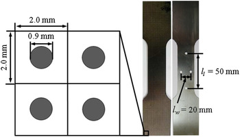
Owing to their crystal structure all metals exhibit some directionality; in particular rolled sheets exhibit direction-dependent material behavior. To determine material anisotropy for zircaloy-4 by tensile tests, we print a grid of circles of diameter 0.9 and 2 mm distance between circles on the tensile specimen (Fig. 1). Grids on metal specimens are usually printed by electro-chemical etching, but due to high corrosion resistance of zircaloy-4, silk-screen printing is used instead. The anisotropy ratio is then calculated from the residual deformation of the grid. To measure strains, marks are printed on the specimen (Fig. 1); the (initial) distances between marks are l l = 50 mm in length direction and l w = 20 mm in width direction. From the corresponding strains (εl and εw, respectively), we calculate the anisotropic ratio r (=εw/εt), where εt is the strain in thickness direction. Assuming incompressibility of plastic deformation, the plastic strain components are related to each other through εl + εw + εt = 0. The relative elongation up to necking is evaluated to 8% for zircaloy-4. Anisotropy is decomposed into normal and planar anisotropy. The normal anisotropy ratio r n is calculated by averaging the anisotropic ratios r 0, r 45, and r 90 where the subscript denotes the angle with respect to the rolling direction (angle to rolling direction, ARD)
 $${r_{\rm{n}}} = {{{r_0} + 2{r_{45}} + {r_{90}}} \over 4}\quad ,$$
henceforth, r n is taken to be the material's anisotropy ratio. We obtain r n = 2.67 for zircaloy-4.
Schematic of grid and tensile test specimen for anisotropic coefficient.

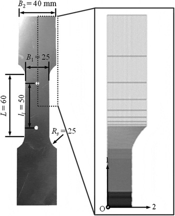
Material properties for zircaloy-4 (Young's modulus E, yield strength σo, fracture strain εf, definition of which will come below, and Poisson's ratio ν) are further obtained by tensile tests. Tensile specimens are manufactured according to KS B0801–5 (Korean Standards Association, Seoul, Korea) with l l = 50 mm and three different ARD (Fig. 2). Tests are conducted on an Instron 5882 tensile testing machine (Instron, Norwood, Massachusetts) with elongation rate of 4.8 mm/min. Displacements are measured via a contactless advanced video extensometer. Young's modulus and yield strength are extracted from the load–displacement curve. Due to the sudden change of the cross sectional area, it is difficult to acquire uniaxial true stress–strain data beyond the necking point. For round specimens, Bridgman Reference Bridgman23 suggested a method to transform the triaxial stress state in the necking region into an equivalent uniaxial stress state, yet, measurement of necessary parameters (radius of curvature and necking cross-section) is problematic. To correct stress–strain curves obtained with flat specimens, Ling Reference Ling24 extrapolated true stress–strain (σt–εt) data after diffuse necking assuming a weighted power law function. The final σt–εt curve is established by varying the weight coefficient w (0 ≤ w ≤ 1) until the analytical engineering stress–strain (σe–εe) curve is in agreement with experimental data. This method has the advantage that a Bridgman-like transformation from a triaxial to a uniaxial stress state is not necessary. Denoting the true stress at diffuse necking by σd and the corresponding true strain by εd, Ling Reference Ling24 proposed the following post-diffuse necking σt–εt relation
 $${\sigma _{\rm{t}}} = {\sigma _{\rm{d}}}\left[ {w\left( {1 + {\varepsilon _{\rm{t}}} - {\varepsilon _{\rm{d}}}} \right) + \left( {1 - w} \right)\left( {{{\varepsilon _{\rm{t}}^{{\varepsilon _{\rm{d}}}}} \over {{\varepsilon _{\rm{d}}}^{{\varepsilon _{\rm{d}}}}}}} \right)} \right]\quad ,$$
if w = 1, the material behavior follows a linear hardening, and if w = 0 it follows a power law function. Linear and power law hardening functions can thus be regarded as upper and lower limits of σt–εt curves. In this study, we refer to Eq. (2) as the weighted-average method (WAM).
Specimen for tensile test and FE model.

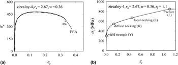
For numerical analysis the commercial software Abaqus 25 is used. The tensile specimen is modeled according to above standard. Considering symmetry, a quarter model is sufficient; it consists of approximately 32,000 8-node brick elements (C3D8 in Abaqus) (Fig. 2). Assuming ARD θ = 0°, the numerical σe–εe curve from Abaqus output is fit to experimental data by varying w in Eq. (2) [Fig. 3(a)] which is Abaqus input. We take the onset of local necking as follows Reference Hyun, Kim, Bang and Lee26
 $$\left| {{\rho _{{\rm{local}}}}} \right| = \left| {{\rho _{P{\rm{max}}}}} \right|\left( {1 - 0.1{{\left. {{\varepsilon _1}} \right|}_{P\max }}} \right)\quad ,$$
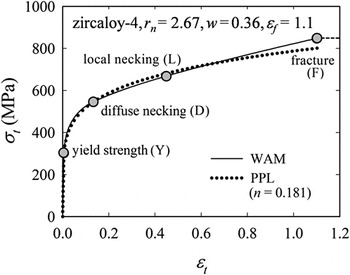
where ρ is the strain ratio (ρ ≡ ε2/ε1). The fracture strain εf is the true major strain corresponding to the fracture displacement in P–δ curve. Reference Hyun, Kim, Bang and Lee26 We obtain εf = 1.1 and w = 0.36 for zircaloy-4. Here w = 0.36 means the material does not follow the pure power law function. Corresponding σt–εt curves are shown in Fig. 3(b), where nonhardening is assumed after εf = 1.1; values for E, σo, and εf obtained from these curves are listed in Table I. Poisson's ratio is usually given in the literature as ν = 0.37 for zircaloy-4.
(a) σe–εe curves and (b) σt–εt curves for zircaloy-4.

Material properties for zircaloy-4.

B. LDH test
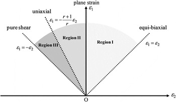
The FLD can be decomposed into three regions (Fig. 4). In Region I, the material is subject to biaxial tension. Diffuse necking occurs at maximum load and the whole sheet becomes uniformly thinner; shortly afterward the material fractures. In Region II, diffuse necking is followed by local necking, i.e., the thickness drops locally; fracture occurs soon afterward. Lastly, when ε2 = −ε1, the sheet is in pure shear. Theoretically, local necking does not occur and the forming limit is predicted with a ductile fracture criterion.
Schematic figure of forming limit diagram.

Experimental FLD's are usually obtained as follows: for positive ε2 (Region I, Fig. 4), the hemispherical punch test proposed by Hecker Reference Hecker27 is applied, while for negative ε2 (Regions II and III, Fig. 4), the flat-headed punch test proposed by Marciniak Reference Marciniak28 is used. However, a disadvantage is that each region of the FLD needs a different test. This problem can be mitigated by using the LDH test proposed by Nakajima workgroup. Reference Hotz29 This test produces the strain states from uniaxial tension [ε1/ε2 = –(r + 1)/r] to biaxial tension (ε1 = ε2) by varying specimen width and lubrication between punch and sheet. Here r is one of r 0, r 45, and r 90.
The limit dome stretch test was originally contrived by Ghosh Reference Ghosh30 and Ayres et al. Reference Ayres, Brazier and Sajewski31 as a test to determine formability. Ghosh subjected rectangular specimens with width of 117–138 mm to displacements. Realizing deformation modes from drawing to stretching, the LDH was expressed by a function of specimen width or minor strain around fracture. Ayres et al. proposed a LDH test-based method to evaluate formability in a relatively simple manner. They noticed that approximately 85–90% of failures occur close to plane strain mode and suggested to use the minimum failure height (LDHo), which is obtained in plane strain, as a stamping formability criterion. Higher dome height means better formability. The Nakajima workgroup Reference Hotz29 of the International Deep Drawing Research Group provided a method that is similar to that of Bragard et al. Reference Bragard, Baret and Bonnarens32 A guideline for the determination of FLC with this method is presented in the other research work. Reference Liebertz, Duwel, Illig, Hotz, Keller, Koehler, Kroeff, Merklein, Rauer, Staubwasser, Steinbeck and Vegter33 It describes in detail the geometry and the number of the specimens, the geometry of the tool and testing conditions such as punch speed, binder force, and lubricant. Major/minor strain pairs are obtained from the grid deformation in the vicinity of local necking. Based on the 3D measurement, some systems have been developed by the commercial company to determine the FLC automatically. Among them, GOM Company has developed the software called ARGUS™ (optical forming analysis) for the determination of FLC. The methodology follows the recommendation of Nakajima workgroup. After the LDH test, the specimen is scanned by ATOS™ (3D digitizing and full-field scanning equipment) and then ARGUS™ calculates the major/minor strains from the image of deformed grids. The strains near crack are then plotted along the 5 path-lines normal to the crack. This approach of using both ATOS™ and ARGUS™ is robust, and shows high repeatability.
C. Experimental FLS determination
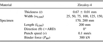
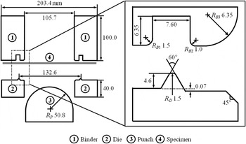
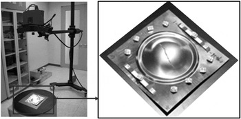
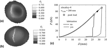
Despite the drawbacks raised by the Nakajima workgroup—namely sensitivity of LDH test to not only specimen shape and ARD but also to grid size and pattern and to the strain measurement method—we follow the ISO 12004-2 (Ref. 34) procedure here. Test conditions are listed in Table II; equipment and notation regarding the LDH test are shown in Fig. 5. To measure the fracture limit for several deformation modes, the specimen length is fixed at l LDH = 200 mm while specimen widths are set to w LDH = 25, 50, 75, 100, 125, 150, 170, 200 mm. ARD is θ = 0° and thickness is t = 0.67 ± 0.01 mm. For the FLD sector of positive minor strain (in biaxial tension), the variation in major/minor strains with specimen width is too small and therefore it is hard to vary the degree of biaxiality by only changing the specimen width. To establish the state of (equi-) biaxial tension and to make the fracture occur close to the dome apex of full-width (square) specimens, lubrication is thus added. For (nearly) full-width specimens as w LDH = 150, 200 mm, we tallow the specimen surface and put a polyethylene foil between dome punch and the tallowed specimen surface to minimize the friction. The same grid as above in Fig. 1 is printed on the specimen. After test, the specimen is scanned by ATOS™ and major/minor strains are calculated from the deformed grid imaged by ARGUS™ (Fig. 6). Figure 7 shows the major strain distributions of zircaloy-4 specimens with width w LDH = 200 mm, from ATOS™, for (i) nonlubrication (ii) lubrication. Also shown in Fig. 7(c) are corresponding LDH test P–δ curves. We state that low friction makes fracture occur near the dome pole while the limiting dome height and the corresponding peak load increase.
Experimental conditions for LDH test.

Schematic figure of LDH test for test tool and drawbead detail.

Strain measuring equipment (ARGUS).

Major strain distributions of zircaloy-4 specimens with w LDH = 200 mm for (a) non-lubrication (b) lubrication and (c) P–δ curves for LDH test depending on lubrication; peak load increases with lubrication.

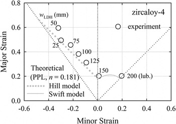
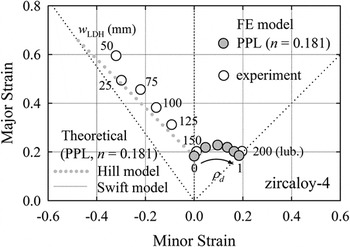
Figure 8 shows the experimental FLS for various specimen widths; theoretical FLC will be explained in detail in Sec. III. The experimental FLS moves in upper left direction with decreasing w. Here, the FLS for w LDH = 25 mm is lower than the one for w LDH = 50 mm, but which seems to be a material characteristic. From Fig. 8 we find that the specimen with w LDH = 150 mm produces a plane-strain state (ε2 = 0) and the lubricated square specimen with w LDH = 200 mm produces an equi-biaxial state (ε1 = ε2). The minor strain increases with specimen width. When using specimens with w LDH > 150 mm, the FLS obtained are nearly the same with the FLS of w LDH = 150 mm. The variation of major/minor strains with the variation of specimen width and lubrication state is very small. Hence, it is hard to obtain experimental data between plane strain and biaxial tension. One method was proposed by Hasek, Reference Hasek35 who introduced arced cutouts into circular LDH test specimens. The arced cutouts cause fracture to occur closer to the center of the specimen and thus closer to the desired combination of principal strains.
Comparison of theoretical FLCs with experimental data.

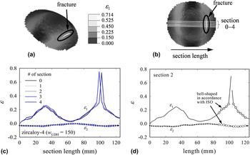
According to ISO 12004-2, FLSs are obtained as follows. After major strains have been determined [Fig. 9(a)], minor and major strains are plotted against the section length measured along the 5 paths [0–4, Fig. 9(b)] passing through the crack [Fig. 9(c)]. The corresponding 5 curve pairs obtained by Gaussian regression are compared, and the curve with the smallest major strain peak from path no. 2 is considered as FLS [Fig. 9(d)]. If there are multiple smallest peaks of major strain, the one with the smallest minor strain value is taken as the critical FLS. When ISO 12004-2 is applied, the evaluated FLS is rather small compared with other methods, for example the one suggested by American Society for Testing and Materials (ASTM). The ISO method has the advantage that results are relatively unaffected by micro necking or fracture length. However, the FLS obtained by ISO 12004-2 is a presumed strain lying somewhere between local necking and ductile fracture and is obtained by Gaussian regression of the strains measured on the fractured specimen. To determine a more appropriate FLS, we will develop a method based on strains measured at the onset of local necking between local thinning and fracture.
Procedure of obtaining FLS (e.g., w LDH = 150 mm) (a) major strain distribution (b) selection for 5 lines in the vicinity of fracture line (c) distribution of major and minor strain with different sections and (d) bell-shaped curve fitting sectional strain.

III. ACQUISITION OF THEORETICAL FLCS
Based on material properties, various theoretical models have been developed for the calculation of FLC. The first ones were proposed by Hill Reference Hill19 (localized necking model) and Swift Reference Swift20 (diffuse necking model) assuming homogeneous sheet metal. Marciniak and Kuczynski (M–K model) Reference Marciniak and Kuczynski21 proposed a model taking into account that sheet metals are nonhomogeneous from both the geometrical and the microstructural point of view. Stören and Rice Reference Stören and Rice22 contrived a model based on the bifurcation theory. In this section, we determine theoretical FLCs for Regions I and II applying Swift's and Hill's models and compare them to the FLSs obtained by LDH tests.
When expressing material behavior by a power law function, the theoretical FLC can be written as Reference Seo, Hyun, Lee and Kim18,Reference Hill19
 $${\varepsilon _1} = \left( {\matrix{ {{n \over {1 + \rho }}} & { \cdots {\rm{ }}{\varepsilon _2} \;\lt \;0} \cr {{{2n\left( {1 + \rho + {\rho ^2}} \right)} \over {\left( {1 + \rho } \right)\left( {2{\rho ^2} - \rho + 2} \right)}}} & { \cdots {\rm{ }}{\varepsilon _2} \;\ge\; 0} \cr} \quad ,} \right.$$
where n is the strain hardening exponent and ρ ≡ ε2/ε1. However, since n does not appear in Eq. (2), the theoretical FLC cannot be obtained from Eq. (4) in combination with Eq. (2). The material data is thus regressed to the following PPL function, which clearly distinguishes between the purely-elastic and elastic–plastic regimes
 $${{{\sigma _{\rm{t}}}} \over {{\sigma _{\rm{o}}}}} = \left( {\matrix{ \,\,{{{{\varepsilon _{\rm{t}}}} \over {{\varepsilon _{\rm{o}}}}}} \hfill & {{\sigma _{\rm{t}}} \;\le\; {\sigma _{\rm{o}}}} \hfill \cr {{{\left( {{{{\varepsilon _{\rm{t}}}} \over {{\varepsilon _{\rm{o}}}}}} \right)}^n}} \hfill & {{\sigma _{\rm{t}}} > {\sigma _{\rm{o}}};\;n\;{\rm{ = 0}}{\rm{.181}}\;{\rm{for}}\;{\rm{zircaloy - 4}}} \hfill \cr} } \right.\quad ,$$
here n, εt , and εo (≡σo/E) are strain hardening exponent, total true strain and yield strain, respectively. σo and E denote initial yield stress and elastic modulus. Figure 10 shows that zircaloy-4 almost obeys the PPL of Eq. (5); we obtain n zircaloy-4 = 0.181. Theoretical FLCs are obtained by inserting n in Eq. (4) (Fig. 8). The theoretical FLC lies somewhat below the experimental curve; however, considering the inevitable errors in experiment, we may state that the theoretical FLC describes the forming limit quite accurately.
Comparison of the σt–εt curves.

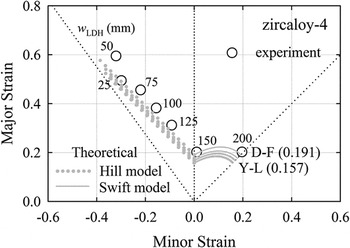
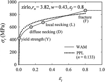
As the parameters in the stress–strain expression are closely related to the formability, the adoption of a suitable stress–strain equation is crucial in the theoretical prediction of FLCs. Figure 11 shows the effect of n on the calculated FLCs for zircaloy-4. When fitting plastic stress–strain data to Eq. (5), we find that n is sensitive to the regression range of strain. To analyze the change of n with the regression range, we select the following six regression ranges: (i) from yield point to diffuse necking (Y–D), (ii) yield point to local necking (Y–L), (iii) yield point to fracture (Y–F), (iv) diffuse necking to local necking (D–L), (v) diffuse necking to fracture (D–F), and (vi) from local necking to fracture (L–F). For each regression range, the values of n are 0.167 (Y–D), 0.157 (Y–L), 0.181 (Y–F), 0.160 (D–L), 0.191 (D–F) and 0.169 (L–F), respectively. There is a large 18% difference between the maximum and minimum values of n that is nonnegligible. Higher n value results in an upward shift of the FLC. More importantly, it is hard to obtain theoretical FLCs for a material not obeying a general power law such as zirlo (Fig. 12). Acquiring theoretical FLCs for non-PPL materials merits a future work.
Comparison of theoretical FLSs with various values of strain hardening exponent.

Comparison of the σt–εt curves for zirlo.

IV. ACQUISITION OF NUMERICAL FLSS
A. Negative minor strain sector (ε2 < 0; between uniaxial tension and plane strain)
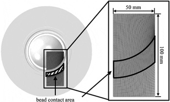
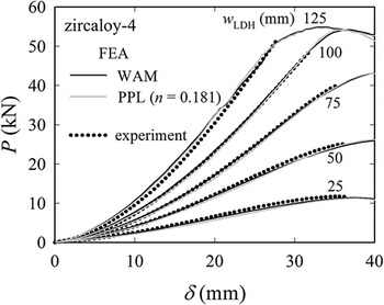
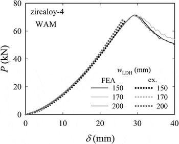
After determining the strain hardening exponent n by regression of stress–strain data to the PPL [Eq. (5)], the theoretical FLC is established. For direct comparison with the FLSs from LDH tests, we obtain in this section numerical FLSs by FE analysis of the LDH test according to ISO 12004-2. Punch, die, and blank holder are fixed; for sheet width w LDH = 100 mm, the FE model of the specimen consists of 15,750 C3D8 elements (Fig. 13). Draw bead is used to hold the sheet, and the punch head is moved toward the upper side. The friction coefficient between the sheet and tools (punch, die and blank holder) is considered with Coulomb friction coefficient of µ = 0.2. Note again that Eq. (2) for zircaloy-4 can also be approximated with Eq. (5) as depicted in Fig. 10. Since the numerical P–δ curves from LDH test simulation using both WAM of Eq. (2) and PPL of Eq. (5) show a good agreement with experimental data (maximum deviation of 3%), we judge Eq. (5) also to be appropriate for zircaloy-4 (Fig. 14).
FE mesh for LDH test (e.g., w LDH = 100 mm).

Comparison of P–δ curves for two different regressed σt–εt curves.

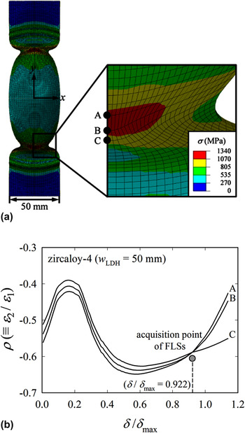
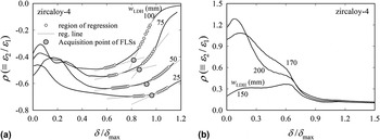
Figure 15(a) shows the Mises stress distribution in the vicinity of the fracture region for w LDH = 50 mm, for example. Point A is the point where fracture occurs. Point B and C are the neighboring nodes below A in y-direction. Figure 15(b) shows the ρ–(δ/δmax) curves from nodes in the vicinity of the fracture region; again ρ ≡ ε2/ε1, and δmax denotes the punch displacement at maximum load. The gray symbol is the loading-point where curve C departs from curves A and B. We may take this loading-point as the initiation of local-necking. The ρ–(δ/δmax) curves at the point A are further plotted for different values of w LDH [Fig. 16(b)]. Following the punch's movement, ρ increases, decreases and increases again; the length of the increasing or decreasing section varies with w LDH. When we observe the region where ρ increases again (after its decrease), the slope first increases gently and then changes abruptly. The intersection of two regression curves for the region of gentle increase and the region of abrupt change may be taken as a numerical FLS acquisition point. Note that the gray symbols for w LDH = 50 mm in Figs. 15(b) and 16(a) provide the same δ/δmax = 0.922. The numerical FLS point can be regarded as the starting point of local thinning. Denoting the displacement at the point of intersection by δc, the ε1 corresponding to δc is taken as FLS. However, the ρ–(δ/δmax) curves for biaxial tension (i.e., for specimens of w LDH = 150, 170, 200 mm) shows no such sudden change in ρ [Fig. 16(b)]. Here, the LDH test P–δ curves overlap (Fig. 17) and experimental FLSs are difficult to determine. We therefore need to find an alternative to obtain FLSs for the sector of ε2 ≥ 0.
(a) Distribution of σ1 at δmax and (b) ρ versus (δ/δmax) curves for w LDH = 50 mm.

ρ versus (δ/δmax) curves for (a) ε2 < 0 and (b) ε2 ≥ 0.

P–δ curves for LDH with w LDH = 150, 170, 200 mm.

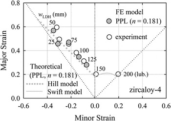
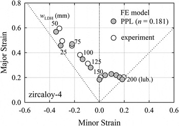
Both numerical and experimental FLSs for ε2 < 0 are depicted in Fig. 18. The numerical ε1 values are somewhat smaller than the experimental ones, but in general, the numerical FLSs are in a good agreement with experimental data. Numerical values are smaller because the experimental critical major strain is a presumed strain (obtained between local necking and ductile fracture), while the numerical critical major strain is obtained at the onset of local thinning.
Comparison of numerical FLSs with experimental FLSs (ε2 < 0).

B. Positive minor strain sector (ε2 ≥ 0; between plane strain and equi-biaxial tension)
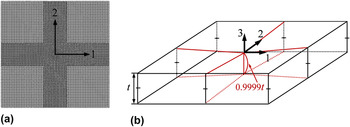
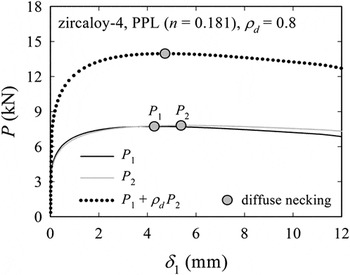
Theoretically, local necking does not occur in the region where ε2 ≥ 0. Therefore, to obtain the FLSs for the biaxial region, we propose a biaxial tensile model and apply diverse displacement ratios ρd (≡δ2/δ1). The FE model of the flat specimen for biaxial tension consists of 35,536 C3D8 elements [Fig. 19(a)]. Length and width of the specimen are 200 mm; thickness is 0.67 mm. To realize necking, we taper the specimen in its center by 0.01% the specimen's thickness [Fig. 19(b)]. Maximum load values obtained using the models with/without taper differ by less than 0.1%, and major and minor strains are equal at maximum load. If the thickness-to-length ratio is sufficiently large, the taper ratio does not affect the P–δ curve or the strain results. For biaxial tension, ρd is set to values between 0 and 1.0 with the interval of 0.2. Invoking that at diffuse necking dP = 0, for uniaxial tension, work W and load P are related by Reference Hill19
 $${{\partial P} \over {\partial \delta }} = {{{\partial ^2}W} \over {\partial {\delta ^2}}} = 0\quad .$$
(a) Biaxial FE mesh for obtaining a FLS [region I (ε2 ≥ 0), Fig. 4] and (b) Schematic diagram of biaxial FE model.

Since ρd = constant, for biaxial tension Eq. (6) can be written as
 $${{\partial W} \over {\partial {\delta _1}}} = {P_1} + {\partial \over {\partial {\delta _1}}}\left[ {\int_{{\rm{ }}0}^{{\rm{ }}{\rho _d}{\delta _1}} {{P_2}\,{\rm{d}}\left( {{\rho _{\rm{d}}}{\delta _1}} \right)} } \right] = {P_1} + {\rho _{\rm{d}}}{P_2}\quad ,$$
where P
1 is a transverse (major) load and P
2 is a longitudinal (minor) load [see Fig. 19(a)]. For ρd ≠ 1, loads and corresponding displacements in major and minor directions are different (Fig. 20). To apply the diffuse necking model, we introduce the relation between work and load, and determine the diffuse necking point. The (effective) load P is then
 $P \,\equiv\, {P_1} + {\rho _{\rm{d}}}{P_2}$
. Consequently, diffuse necking occurs when the following equation is satisfied
 $${{{\partial ^2}W} \over {\partial \delta _1^2}} = {{\partial {P_1}} \over {\partial {\delta _1}}} + {\rho _{\rm{d}}}{{\partial {P_2}} \over {\partial {\delta _1}}} = 0 \leftrightarrow P = {P_{\max }}\quad .$$
P–δ curves with definition of P (e.g., ρd = 0.8).

The numerical FLSs are the major/minor strain pairs satisfying Eq. (8). The gap between the FLSs and the theoretical FLCs are below 5% (Fig. 21).
Comparison of numerical FLSs with experimental FLSs (ε2 ≥ 0).

Figure 22 reveals a good agreement between the numerical and experimental FLSs for the whole range of ε2. Note that as stated in Sec. II. C, it is hard to obtain the distributed data of experimental FLSs in biaxial tension mode (ε2 > 0). Applying our numerical approach to the materials obeying the power law, we further confirmed that our FE approach is valid for general materials. However, those data are omitted here, as this paper focuses only on zirconium alloys. In the near future, the matter will be reported in detail. Therefore, our FE approach can both substitute and supplement experimental LDH tests which are the expensive and time-demanding.
Comparison of numerical FLSs with experimental FLSs for all regions of ε2.

V. CONCLUSION
We studied the FLSs and FLCs for zircaloy-4 sheets. First, material properties and anisotropic ratio were evaluated by tensile tests. LDH tests were performed to produce experimental FLSs. The material stress–strain curves were regressed to power–law functions for determination of theoretical FLC, and it was shown that hardening exponent n varies largely with the regression range of strain. On this base, a numerical method to determine FLSs was proposed to obviate the problem related with theoretical FLSs. We obtained numerical FLSs for ε2 < 0 sector by simulating the LDH test and for ε2 ≥ 0 sector with the biaxial tension model. The procedures of finding numerical FLS point are elaborated in Figs. 16(a) and 20. The numerical FLSs were in a good agreement with experimental data for both sectors. We note again that numerical FLSs are the strains at the point of local thinning, while experimental FLSs are the strains presumed between local thinning and fracture. In conclusion, our FE approach can substitute the experimental LDH tests, which are expensive and time-demanding and not applicable to the ε2 ≥ 0 sector.
ACKNOWLEDGMENTS
This work was supported by the Nuclear Power Core Technology Development Program of the Korea Institute of Energy Technology Evaluation and Planning (KETEP), granted financial resource from the Ministry of Trade, Industry and Energy, Republic of Korea. (No. KETEP-2013 85400 40010)