1 Introduction
Free-electron lasers (FELs) are devices that efficiently convert the kinetic energy from a relativistic electron beam into energy in the form of electromagnetic radiation. They are known to produce radiation in a wide region of the spectrum (Marshall Reference Marshall1985; Bonifacio et al. Reference Bonifacio, Casagrande, Cerchoni, de Salvo Souza, Pierini and Piovella1990; Brau Reference Brau1990; Freund & Antonsen Reference Freund and Antonsen1996).
In a FEL, a relativistic electron beam co-propagates with a very small initial signal electromagnetic wave (EMW), called laser or radiation. The electrons pass within a spatially periodic magnetic field produced by a wiggler. The electrons of the beam interact with the external magnetic field, with the EMW and with themselves. The superposition of the laser and wiggler fields forms what is known as the ponderomotive potential. If the initial conditions (energy of the beam, wavelengths of the fields and wiggler field amplitude) are correct, as the electrons are entrapped by the ponderomotive potential, they lose energy and deliver this energy to the laser field. The process makes the radiation grow exponentially until nonlinear effects, such as the space-charge, begin to dominate the system dynamics (Sprangle, Tang & Manheimer Reference Sprangle, Tang and Manheimer1980; Bonifacio et al. Reference Bonifacio, Casagrande, Cerchoni, de Salvo Souza, Pierini and Piovella1990; Seo & Choi Reference Seo and Choi1997; Wang, Xiao & Liang Reference Wang, Xiao and Liang2006; Monteiro et al. Reference Monteiro, Serbeto, Tsui, Mendonça and Galvão2013; Peter et al. Reference Peter, Endler, Rizzato and Serbeto2013; Peter, Endler & Rizzato Reference Peter, Endler and Rizzato2014).
Much work has been done in order to estimate analytically the growth rate of the laser field either in the (hypothetical) case of an initially monoenergetic electron beam (Sprangle et al. Reference Sprangle, Tang and Manheimer1980; Murphy, Pellegrini & Bonifacio Reference Murphy, Pellegrini and Bonifacio1985; Seo & Choi Reference Seo and Choi1997; Peter et al. Reference Peter, Endler, Rizzato and Serbeto2013) or in the case of an initial energy distribution (Ibanez & Johnston Reference Ibanez and Johnston1983; Freund, Davidson & Kirkpatrick Reference Freund, Davidson and Kirkpatrick1991; Babaei & Maraghechi Reference Babaei and Maraghechi2008; Chakhmachi & Maraghechi Reference Chakhmachi and Maraghechi2009; Peter et al. Reference Peter, Endler and Rizzato2014). In a recent work, we linearized the wave–particle set of equations for a one-dimensional (1D) FEL including the space-charge effects, and then we added a pressure term ad hoc, related to the half-width of the initial water-bag velocity distribution in the linear system. Through the Vlasov equation and its moments, it was possible to connect the pressure of the beam and the fluctuations of the energy of the particles. The pressure of non-relativistic water-bag distribution is well known in the literature (Coffey Reference Coffey1971) and has been proved to work well in the hydrodynamical regime, i.e. for very small initial spreads (Peter et al. Reference Peter, Endler and Rizzato2014).
This work is an extension of a recent one (Peter et al. Reference Peter, Endler and Rizzato2014). Here we generalize the results for different and symmetrical initial distributions for the longitudinal velocity of the particles. The generalization is made through the definition of the equivalent initial spread. The equivalent spread is obtained by considering the beam as a warm fluid composed of different fluids with different densities with water-bag initial distributions. Thus, the initial distribution could be composed of a sum of water bags, as a layered model. As an example we make use of the Gaussian distribution. We show that via linear analysis it is possible to estimate the detuning to maximize the growth rate of the laser field and also the evolution of the laser field during the linear regime. A comparison is made between the results given by the wave–particle equations and the linear analysis. We point out that this kind of approach is much less complicated than the traditional kinetic one.
The paper is organized as follows: in § 2, we present the physical model with the wave–particle equations to describe the 1D FEL; in § 3, we introduce the concept of equivalent initial spread; in § 4, we apply this concept to the linearized set of equations; in § 5, we compare the results given by the wave–particle equations and the linear analysis; finally, in § 6, we draw our conclusions.
2 Physical model
The physical model presented here was developed in a recent paper (Peter et al. Reference Peter, Endler, Rizzato and Serbeto2013). The notation and the normalization differ from Bonifacio et al. (Reference Bonifacio, Casagrande, Cerchoni, de Salvo Souza, Pierini and Piovella1990). However, the set of equations presented in this work reproduces the results and the physics of 1D FELs. Thus, only the final expressions for the equations are shown.
The wiggler
 $(\boldsymbol{A}_{w})$
and the laser
 $(\boldsymbol{A})$
fields are described by their vector potential fields, respectively
 $$\begin{eqnarray}\displaystyle & \displaystyle \frac{e\boldsymbol{A}_{w}}{mc^{2}}=a_{w}(z)\hat{\boldsymbol{e}}\exp [\text{i}(\boldsymbol{k}_{w}z)]+\text{c.c.}, & \displaystyle\end{eqnarray}$$
 $$\begin{eqnarray}\displaystyle & \displaystyle \frac{e\boldsymbol{A}}{mc^{2}}=a(z)\hat{\boldsymbol{e}}\exp [\text{i}(\boldsymbol{k}z-{\it\omega}t)]+\text{c.c.}, & \displaystyle\end{eqnarray}$$
 $\boldsymbol{k}_{w}$
and
 $\boldsymbol{k}$
are the wavevector of the wiggler and the laser;
 ${\it\omega}$
is the frequency of the radiation;
 $a=a(z)$
is the slowly varying dimensionless amplitude of the laser and
 $a_{w}$
is the dimensionless undulator parameter; and
 $\hat{\boldsymbol{e}}$
is the circular polarization versor.
An energy,
 ${\it\gamma}$
, and a phase,
 ${\it\theta}$
, equation are necessary to describe the evolution of the particles. The energy is a function of the amplitude of the laser and wiggler fields and of the longitudinal velocity of the electrons, while the phase is the phase of the particles inside the ponderomotive potential. According to the phase of the particle, the particle can be accelerated or decelerated by the ponderomotive potential. If the particle is accelerated (decelerated), then energy is drained (delivered) from (to) the laser field. To describe the evolution of the radiation field,
 $a(z)$
, a wave equation is obtained. The final expressions for the wave–particle set of equations of the FEL are written as (
 $t={\it\omega}t$
,
 $v=v/c$
and
 $z=v_{p}t=\boldsymbol{k}/(\boldsymbol{k}+\boldsymbol{k}_{w})t$
)
 $$\begin{eqnarray}\displaystyle & \displaystyle \frac{\text{d}}{\text{d}z}{\it\gamma}_{j}=-\frac{a_{w}}{2{\it\gamma}_{j}}[a\text{e}^{\text{i}{\it\theta}_{j}}+\text{c.c.}]+{\it\eta}^{2}v_{p}v_{z,j}\left\langle -({\it\theta}_{k}-{\it\theta}_{j})+{\rm\pi}\frac{({\it\theta}_{k}-{\it\theta}_{j})}{|{\it\theta}_{k}-{\it\theta}_{j}|}\right\rangle , & \displaystyle\end{eqnarray}$$
 $$\begin{eqnarray}\displaystyle & \displaystyle \frac{\text{d}}{\text{d}z}{\it\theta}_{j}=\frac{v_{z,j}}{v_{p}(1-{\it\nu})}-1, & \displaystyle\end{eqnarray}$$
 $$\begin{eqnarray}\displaystyle & \displaystyle \frac{\text{d}}{\text{d}z}a={\it\eta}^{2}v_{p}a_{w}\left\langle \frac{\text{e}^{-\text{i}{\it\theta}}}{2{\it\gamma}}\right\rangle -\text{i}{\it\eta}^{2}v_{p}\left\langle \frac{1}{2{\it\gamma}}\right\rangle a. & \displaystyle\end{eqnarray}$$
In these equations, the quantity
 ${\it\eta}$
is the space-charge factor arising from the beam charge
 ${\it\eta}^{2}={{\it\omega}_{p}}^{2}/{\it\omega}^{2}$
, with
 ${\it\omega}_{p}=\sqrt{4{\rm\pi}n\text{e}^{2}/m}$
being the plasma frequency and
 $n$
being the average density of particles;
 ${\it\nu}$
is the detuning, which is a dimensionless parameter that measures somehow the difference between the ponderomotive potential velocity and the mean beam velocity; the velocity of the ponderomotive potential is represented by
 $v_{p}=\boldsymbol{k}/(\boldsymbol{k}_{w}+\boldsymbol{k})=\boldsymbol{k}/\boldsymbol{k}_{p}<1$
; the brackets indicate an average over the particle distribution; and the longitudinal particle velocity is given through the relativistic Lorentz factor definition:
 $v_{z}=[1-(1-|a_{tot}|^{2})/{{\it\gamma}_{j}}^{2}]^{1/2}$
, with
 $|a_{tot}|^{2}=|a_{w}(\exp [\text{i}(\boldsymbol{k}_{w}z)]+\text{c.c.})+(a\exp [\text{i}(\boldsymbol{k}z-{\it\omega}t)]+\text{c.c.})|^{2}$
. Moreover, using the Poynting vector, it is possible to find a relation in which the normalized density of energy,
 ${\it\epsilon}$
, is conserved. This relation is given by:
 ${\it\eta}^{2}\langle {\it\gamma}\rangle +|a|^{2}={\it\epsilon}$
(or, in the original variables of the problem:
 $n\langle {\it\gamma}\rangle mc^{2}+|E|^{2}/4{\rm\pi}={\it\epsilon}^{\ast }$
) (Bonifacio et al.
Reference Bonifacio, Casagrande, Cerchoni, de Salvo Souza, Pierini and Piovella1990).
This set of equations, (2.3)–(2.5), describe the evolution of the particles and the laser field of 1D FEL dynamics. The different longitudinal velocity distributions are introduced in these equations through the initial conditions. In the next section, we introduce the concept of equivalent initial spread and provide the theoretical ground to support the analysis.
3 Equivalent initial spread
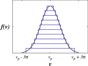
In the hydrodynamical regime, we assume the initial distributions could be composed of a sum of water-bag distributions, with different half-widths (
 ${\rm\Delta}v_{0}$
), as shown in figure 1 (it is important to notice that each water-bag distribution has an area in the
 $f(v)\times v$
space). The sum of water bags imposes that the initial distribution must be symmetrical, because each water-bag distribution must be centred in a specific longitudinal velocity. The sum of water bags is analogous to considering that the warm beam is composed of different fluids, where each fluid has constant density over the occupied phase space. Moreover, we assume that the dynamics of each fluid is laminar in the phase space (
 ${\it\gamma}\times {\it\theta}$
or
 $v_{z}\times {\it\theta}$
) until the nonlinearities begin to dominate the system dynamics. Then, they are exactly represented by adiabatic fluid equations, (Coffey Reference Coffey1971) as long as the laminar regime persists: more than that, the system evolutes as each fluid is separated from the others. The superposition of fluids, which could be thought of as a layered model, sounds like a reasonable simplification of the physical model.
The equivalent initial spread (or, equally, the equivalent temperature),
 ${{\rm\Delta}v_{0}}_{eq}$
, is a sum of the contributions of each of these fluids. The contribution given by each fluid depends on the density of particles of the fluids. This implies that if we look at the normalized distribution function,
 $f(v)$
, the contribution of each fluid is given by the half-width of the fluid and the area that the fluid occupies. Thus, we write
 $$\begin{eqnarray}{{\rm\Delta}v_{0}}_{eq}=\mathop{\sum }_{1}^{N}{\rm\Delta}v_{0,i}A_{i},\end{eqnarray}$$
where
 $A_{i}$
is the area of the
 $i$
th water-bag distribution and
 $N$
is the number of layers (water-bag distributions composing the original distribution) with the normalization condition that
 $A=\sum _{1}^{N}A_{i}=1$
, where
 $A$
is the total area below the distribution curve.
On the other hand, the
 $i$
th area is a function of
 ${\rm\Delta}v_{0,i}$
and is limited by the thickness considered for
 $f(v)$
, which is expressed by
 $s=f_{max}/N$
, where
 $s$
is the thickness considered for
 $f(v)$
;
 $f_{max}$
is the maximum value of
 $f(v)$
; and
 $N$
is the number of water-bag distributions used to compose the original distribution.
The vertical axis represents the distribution function
 $f(v)$
, while the horizontal axis shows the velocity. The distribution function (a Gaussian distribution, in this case) is divided into water-bag distributions, which are delimited by the blue solid lines.

As an example of distribution, we take a Gaussian distribution. Typically, the Gaussian distribution function,
 $f_{g}(v)$
, is expressed as
 $$\begin{eqnarray}f_{g}(v)=C\text{e}^{-(v-\bar{v})^{2}/2{\it\sigma}^{2}},\end{eqnarray}$$
where
 ${\it\sigma}$
is the standard deviation,
 $C$
is a normalization constant,
 $C=1/\int \text{e}^{-(v-\bar{v})^{2}/2{\it\sigma}^{2}}\text{d}v$
, and
 $\bar{v}$
is the mean velocity. Gaussian distributions for the initial velocities are symmetrical in relation to the mean velocity, as can be seen in (3.2). Due to numerical limitations, we considered a distribution between
 $\bar{v}-3{\it\sigma}$
and
 $\bar{v}+3{\it\sigma}$
.
On the other hand, the water-bag distribution
 $f_{wb}$
is a uniform distribution over the velocity spread:
 $f_{wb}(v)=(2{\rm\Delta}v_{0})^{-1}$
, where
 ${\rm\Delta}v_{0}$
is the half-width of the distribution.
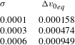
In table 1 we show the variance of the Gaussian distribution
 ${\it\sigma}$
and its equivalent spread
 ${{\rm\Delta}v_{0}}_{eq}$
.
Variance of the Gaussian distribution
 ${\it\sigma}$
and its equivalent spread
 ${{\rm\Delta}v_{0}}_{eq}$
.

4 Linear analysis
The electron beam is injected with a co-propagating radiation field, in such a way that the initial amplitude of the laser is very small in comparison with the wiggler field. Then, the radiation field is considered a perturbation of the wiggler one. The radiation and the wiggler fields cause perturbations in the other physical quantities (phase and energy) around the equilibrium values (the equilibrium values are obtained from the zeroth-order solutions of the equations).
In this section, we present a linear analysis based on those perturbations, which implies a linearization of the complete set of equations (Bonifacio et al. Reference Bonifacio, Casagrande, Cerchoni, de Salvo Souza, Pierini and Piovella1990; Peter et al. Reference Peter, Endler, Rizzato and Serbeto2013, Reference Peter, Endler and Rizzato2014). The linear analysis provides the growth rate of the laser field during the linear regime. Instead of using the original physical quantities, we made use of the collective variables. The collective variables represent the fluctuations of the phase and the energy.
Thus, the linear evolution of the radiation field is obtained through the integration of the following set of equations
 $$\begin{eqnarray}\displaystyle & \displaystyle {\dot{X}}=\text{i}\left[\frac{a_{w}}{2{v_{p}}^{2}(1-{\it\nu}){{\it\gamma}_{r}}^{2}}\right]\tilde{a}+\left[\frac{1+{a_{w}}^{2}}{{v_{p}}^{2}(1-{\it\nu}){{\it\gamma}_{r}}^{3}}\right]Y, & \displaystyle\end{eqnarray}$$
 $$\begin{eqnarray}\displaystyle & \displaystyle \dot{\tilde{a}}=-\left[v_{p}\frac{a_{w}{\it\eta}^{2}}{2{\it\gamma}_{r}}\right]\left(\text{i}X+\frac{Y}{{\it\gamma}_{r}}\right)-\text{i}\left(v_{p}\frac{{\it\eta}^{2}}{2{\it\gamma}_{r}}-{\it\nu}\right)\tilde{a}, & \displaystyle\end{eqnarray}$$
 $$\begin{eqnarray}\displaystyle & \displaystyle {\dot{Y}}=-\frac{a_{w}}{2{\it\gamma}_{r}}\tilde{a}-{v_{p}}^{2}{\it\eta}^{2}X+{\dot{Y}}|_{warm}, & \displaystyle\end{eqnarray}$$
 $X$
represents the fluctuations in the phase (
 $X=\langle \text{e}^{-\text{i}\tilde{{\it\theta}}_{0}}{\it\delta}\tilde{{\it\theta}}\rangle$
); the collective complex variable
 $Y$
represents the fluctuations in the energy (
 $Y=\langle \text{e}^{-\text{i}\tilde{{\it\theta}}_{0}}{\it\delta}{\it\gamma}\rangle$
);
 $\tilde{a}$
is the transformed complex laser amplitude (
 $\tilde{a}\text{e}^{\text{i}\tilde{{\it\theta}}}=a\text{e}^{\text{i}{\it\theta}}$
);
 $\tilde{{\it\theta}}$
is the transformed phase
 $({\it\theta}=\tilde{{\it\theta}}-{\it\nu}z)$
;
 ${\it\gamma}_{r}=[(1+|a_{tot}(z=0)|^{2})/(1-{v_{p}}^{2})]^{1/2}$
is the resonant energy; and
 ${\dot{Y}}|_{warm}$
is the ad hoc pressure term due to thermal effects.
With these coupled equations it is possible to generate a third-order polynomial equation to determine the parameters that lead to the maximum growth rate. The linear set of equations also provides the linear growth of the laser amplitude.
The ad hoc pressure term is obtained through the Vlasov equation and its moments for each fluid exactly as in Peter et al. (Reference Peter, Endler and Rizzato2014). It reads
 $$\begin{eqnarray}{\dot{Y}}|_{warm}=-\frac{{{\rm\Delta}{v_{0}}_{eq}}^{2}}{2D_{{\it\gamma}^{2}}{\it\gamma}_{0}}X,\end{eqnarray}$$
where
 $D_{{\it\gamma}^{2}}=\partial ^{2}v/\partial {\it\gamma}^{2}$
evaluated at the injection.
5 Results
5.1 Detuning to maximize the growth rate
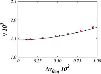
As already mentioned, linear analysis provides the linear growth rate of the laser field. Then, it is possible to determine the detuning which maximizes the growth rate. This detuning is obtained through either the integration of the linear system of equations or the cubic polynomial, assuming solutions of the laser amplitude as
 $a(z)\propto \text{e}^{\text{i}{\it\tau}z}$
. The imaginary part of the complex roots of
 ${\it\tau}$
corresponds to the slope of the
 $\text{log}|a|$
evolution along
 $z$
.
Detuning
 ${\it\nu}$
to maximize the laser growth rate versus the equivalent initial velocity spread. The solid line is from the linear analysis. Black (red) filled circles are the results of the wave–particle simulations for the water-bag (Gaussian) distribution.

The detuning that maximizes the radiation growth rate is shown versus the equivalent spread in figure 2 for
 $a_{w}=0.4$
;
 $a(z=0)=\text{i}a_{w}10^{-5}$
;
 $v_{p}=0.99$
; and
 ${\it\eta}=0.03$
(these values are kept constant during this paper – the role of the space-charge effect was already discussed in Peter et al. (Reference Peter, Endler and Rizzato2014)). The solid line is the result obtained through the linear analysis, while the black filled circles are obtained via the integration of the wave–particle equations for a water-bag distribution, using 20 000 particles. The red filled circles are from the integration of the wave–particle equations for a Gaussian distribution, with its corresponding equivalent spread, using 40 000 particles. The results show a reasonable agreement between the different distributions.
A small discrepancy is seen for values of
 ${\rm\Delta}v_{0}$
bigger than
 $0.0007$
. This point forward, the deviation,
 ${\it\sigma}$
, of the Gaussian distribution is big enough that an increasing fraction of particles ceases to deliver energy to the laser field. It occurs because these particles have velocities very different to the ponderomotive potential one (remembering that the Gaussian distribution is distributed over a larger velocity range in comparison to the water-bag distribution), therefore the ponderomotive potential is not able to trap them.
5.2 Slope of the linear growth rate
Although the detuning which maximizes the radiation growth rate is similar between the distributions, the effective value of the laser growth rate must be compared. The radiation growth is almost linear until the breakdown of the laminar regime. Thus the logarithm of the modulus of the laser field amplitude (
 $\text{log}|a|$
) could be fitted to a straight line, where
 ${\it\tau}$
is the slope – corresponding to the growth of the laser field.
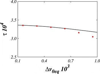
In figure 3, the growth rate
 ${\it\tau}$
of the laser field is compared for the different distributions, over the curve of maximum growth rate shown in figure 2. The solid black line was obtained through wave–particle simulations of water-bag distributions, while the red filled circles were obtained from the wave–particle simulations of Gaussian distributions.
The linear coefficient of the growth rate,
 ${\it\tau}$
, is plotted versus the equivalent initial spread
 ${\rm\Delta}v_{0}$
. The solid line is from water-bag distributions and the filled circles are from Gaussian distributions. The results were performed through wave–particle simulations. The detuning
 ${\it\nu}$
is the detuning that maximizes the growth rate.

The results agree well until
 ${\rm\Delta}v_{0}\approx 0.0007$
. The reason is similar to the one presented in the discussion about the detuning to maximize the growth rate.
5.3 Evolution of the phase space
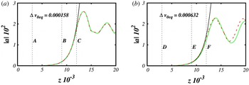
In the laminar regime, the radiation field grows exponentially and the beam could be thought of as a sum of fluids with different densities. In this regime, we saw linear analysis provide the laser growth rate in a reasonable fashion. In figure 4, we show the evolution of the amplitude of the laser field for two different values of
 ${\rm\Delta}v_{0}$
: in (a),
 ${\rm\Delta}{v_{0}}_{eq}=0.000158$
, while in (b),
 ${\rm\Delta}{v_{0}}_{eq}=0.000632$
. The green solid (red dashed) line is the wave–particle simulation evolution of the laser field for the Gaussian (water-bag) initial distribution, while the black solid line is the solution of the linear set of equations. In these figures is possible to see that the linear analysis represents quite well the evolution of the laser field in the beginning of the system dynamics. The curves start to split, approximately, in the
 $z$
corresponding to the breakdown of the laminar regime.
The evolution of the radiation field versus
 $z$
. The green solid (red dashed) line represents the wave–particle solution for the Gaussian (water-bag) initial distribution. The black solid line is the solution of the linear set of equations. (a) Was built for
 ${\rm\Delta}{v_{0}}_{eq}=0.000158$
, while (b) was built for
 ${\rm\Delta}{v_{0}}_{eq}=0.000632$
. The indexed vertical dashed lines denote snapshots of the system for the corresponding
 $z$
in figure 5.

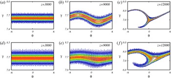
Snapshots of the phase space at different
 $z$
’s. (a) and (d) were built for
 $z=3000$
, (b) and (e) were built for
 $z=9000$
and (c) and (f) are for
 $z=12\,000$
. Moreover, (a–c) were made for
 ${\rm\Delta}{v_{0}}_{eq}=0.000158$
, while (d–f) were made for
 ${\rm\Delta}{v_{0}}_{eq}=0.000632$
. The colours indicate the density of particles, varying from blue (smaller densities) to red (bigger densities).

With a view to confirming that the evolution of the system is well described in the laminar regime, in figure 5 we show the evolution of the phase-space configuration along
 $z$
for different initial spreads and different initial distributions. The colours indicate the local density, varying from blue (smaller) to red (bigger) values of density. The density was measured through the discretization of the phase space in a mesh of
 $150\times 150$
pixels. Then, the number of particles in each pixel represent somehow the local density of particles. (a–c) correspond to
 ${\rm\Delta}{v_{0}}_{eq}=0.000158$
, while (d–f) correspond to
 ${\rm\Delta}{v_{0}}_{eq}=0.000632$
. Moreover, (a) and (d) were built for
 $z=3000$
, (b) and (e) were built for
 $z=9000$
and, finally, (c) and (f) were built for
 $z=12\,000$
.
In panels (a–e), the system is in the linear regime. Thus, the superposition of the fluids and linear theory is valid. We can see from the colours that the flow of particles is laminar. Moreover, the panels suggest the sum of fluids is possible because the density of each fluid is constant as long as the laminar regime persists in the phase space. It gives the model proposed in this work a physical meaning.
On the other hand, after the breakdown of the laminar regime – which occurs when the lower border of the distribution starts to twist around itself in the phase space (Peter et al. Reference Peter, Endler and Rizzato2014) – the beam cannot be thought of as a sum of fluids and the density of each fluid is not constant any more.
6 Conclusions
In this work, we estimate the linear growth rate of the laser field in FELs, including space-charge and thermal effects through the linearization of the wave–particle set of equations. In a recent paper (Peter et al. Reference Peter, Endler and Rizzato2014), the linear growth rate was reasonable predicted for a water-bag initial distribution for the longitudinal velocity of the particles in the hydrodynamical regime. In this regime, the warm electron beam would be thought of as a fluid. Furthermore, in the case of a very small initial spread, it was possible via the Vlasov equation to identify the pressure term of the fluid and to add an ad hoc term in the linear set of equations related to the initial distribution. The main advantage of this approach in relation to the kinetic one is that the first one is much less complicated in terms of calculations.
Here, we extended the results for different symmetrical initial distributions (we took the Gaussian distribution function as an example), assuming that, in the hydrodynamical regime, the distributions could be represented by a sum of water-bag distributions. This is equivalent to assuming a superposition of different fluids with different densities to represent the beam. A relation between the pressures and the densities of the fluids was obtained, suggesting an equivalent initial spread between the distributions.
We compared the results given by the linear analysis and the wave–particle simulations, for a fixed value of
 ${\it\eta}$
. The linear growth rate and the detuning to maximize the growth rate agree well in the limit of very small spreads (
 ${\rm\Delta}{v_{0}}_{eq}<{\it\nu}$
). Moreover, the evolution of the phase space at different
 $z$
from wave–particle simulations shows that the superposition of the fluids reasonably reproduces the physics of the system until the breakdown of the laminar regime.
Although this linear analysis provided good results, given its simplicity, the analysis is limited to very small initial spreads – which is, in fact, realistic for FELs (Chakhmachi & Maraghechi Reference Chakhmachi and Maraghechi2009). To completely include the thermal effects in the analysis, a more sophisticated approach must be used. One of the ways to do that is to make a kinetic description. This issue and others shall be further studied in coming works.
Acknowledgements
This work was supported by CNPq and FAPERGS, Brazil, and by the Air Force Office of Scientific Research (AFOSR), USA, under the grant FA9550-12-1-0438. The authors wish to thank R. Pakter, S. Marini and A. Serbeto for useful discussions.