1. Introduction
The concept of ageing is attracting the attention of an increasing number of lifetime researchers (see, e.g., [Reference Bhattacharjee, Nanda and Misra4, Reference Deshpande, Kochar and Singh11, Reference Jiang, Ji and Xiao12, Reference Szymkowiak26]). Properties of a random lifetime are usually described by means of the respective absolutely continuous distribution function F with density  $f(x){\kern 1pt} = {\kern 1pt} {{dF(x)} \over {dx}}$ supported on the positive half-axis. A classical tool of lifetime analysis is the failure rate
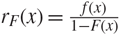 ${r_F}(x) = {{f(x)} \over {1 - F(x)}}$, x > 0, also known as the hazard rate function. Related notions are the cumulative failure rate (often called the hazard function)
 ${R_F}(x) = \int_0^x {r_F}(t){\kern 1pt} dt$ and the average failure rate
 ${H_F}(x) = {1 \over x}\int_0^x {r_F}(t){\kern 1pt} dt$
.
The tool that was especially designed for gauging the ageing tendency is the ageing intensity function
 $${L_F}(x) = {{{r_F}(x)} \over {{H_F}(x)}} = {{ - xf(x)} \over {(1 - F(x))\ln (1 - F(x))}}\quad \quad for\;x \in (0, + \infty ),$$
proposed in [Reference Jiang, Ji and Xiao12]. The ageing intensity is defined as the ratio of the instantaneous failure rate rF to the average failure rate HF, and expresses the relation between the actual inclination of an item for dying and its average ageing tendency in the past. It describes the ageing property quantitatively: the larger the ageing intensity, the stronger the ageing tendency. Reference [Reference Szymkowiak26] proved that the ageing intensity (1) characterizes a scale family of lifetime distributions.
It was noted in [Reference Szymkowiak27] that the ageing intensity 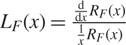 ${L_F}(x) = {{{d \over {dx}}{R_F}(x)} \over {{1 \over x}{R_F}(x)}}$ can be treated as the elasticity ERF (x) of the non-decreasing positive cumulative failure rate function. Elasticity is an important economic notion, and a thorough discussion of it can be found in [Reference Sydsæter and Hammond25]. The ageing intensity LF measures the percentage by which the cumulative failure rate function RF increases when the time x increases by a small amount.
It is sometimes assumed that lifetime random variables have distributions with supports bounded above. In some applications, although in few practical situations, one needs to assume that an item under investigation survives a given initial time interval for certain, and then dies (fails) at some random time afterwards. Therefore in this paper we consider general absolutely continuous lifetime distribution functions, say F, with respective positive density functions f on an interval support (lF, uF) such that 0 ≤ lF < uF ≤+∞. Then the ageing intensity function of F can be written as
 $${L_F}(x) = \left\{ {\matrix{
0 \hfill & {for} \hfill & {x \lt {l_F},} \hfill & {} \hfill \cr
{{{{r_F}(x)} \over {{H_F}(x)}}} \hfill & {for} \hfill & {{l_F} \le x \le {u_F},} \hfill & {} \hfill \cr
{ + \infty } \hfill & {for} \hfill & {x > {u_F}} \hfill & {} \hfill \cr
} } \right.$$
(see [Reference Bhattacharjee, Nanda and Misra4]). Reference [Reference Szymkowiak27] introduced the notion of the G-generalized ageing intensity function for the distribution function F supported on the whole of (0, +∞) defined by the formula
 $${L_{G,F}}(x) = {{x\;{r_{G,F}}(x)} \over {{R_{G,F}}(x)}},\quad \quad 0 \lt x \lt + \infty ,$$
where G is another strictly increasing absolutely continuous lifetime distribution function. The functions RG,F = (G −1 ∘ F)(x) and  ${r_{G,F}}(x) = {{\rm{d}} \over {{\rm{d}}x}}{R_{G,F}}(x)$ are called the G-generalized cumulative failure rate and the G-generalized failure rate, respectively. They were defined and studied in [Reference Barlow and Van Zwet1, Reference Barlow and Van Zwet2, Reference Barlow and Van Zwet3] (see also [Reference Chang7, Reference Cheng8, Reference Shaked23] for further developments). Observe that formulae (1) and (3) are equivalent for G(x) = 1 − exp (−x), x ∊ (0, +∞), the standard exponential distribution (see [Reference Marshall and Olkin17]).
Here we assume that F, G are absolutely continuous lifetime distribution functions supported on intervals (lF, uF) ⊂ (0, +∞) and (lG, uG) ⊂ (0, +∞), respectively. Then the G-generalized failure rate of F can be defined as
 $${r_{G,F}}(x) = {{\rm{d}} \over {{\rm{d}}x}}({G^{ - 1}} \circ F)(x) = {{f(x)} \over {(g \circ {G^{ - 1}} \circ F)(x)}},\quad \quad {l_F} \lt x \lt {u_F},$$
where f and g stand for the density functions of F and G, respectively. The corresponding G-generalized cumulative hazard function of F is the strictly increasing transformation RG,F :(lF, uF) ↦ (lG, uG) defined by RG,F = G −1 ∘ F. Another useful notion in lifetime analysis is the G-generalized average failure rate,
 $${H_{G,F}}(x) = {{{R_{G,F}}(x)} \over x} = {{({G^{ - 1}} \circ F)(x)} \over x},\quad \quad {l_F} \lt x \lt {u_F}.$$
Ultimately, we introduce the G-generalized ageing intensity of F as follows:
 $${L_{G,F}}(x) = {{{r_{G,F}}(x)} \over {{H_{G,F}}(x)}} = {x \over {({G^{ - 1}} \circ F)(x)}}{\kern 1pt} {{f(x)} \over {(g \circ {G^{ - 1}} \circ F)(x)}},\quad \quad {l_F} \le x \le {u_F}.$$
This takes on values in (0, +∞), and for various choices of G it measures various aspects of the ageing tendency of a lifetime random variable with distribution function F at time x: the greater the value of LG,F at x, the greater the susceptibility of an item with lifetime distribution F to die at x rather than at some other time. A natural extension of ageing intensity functions onto the whole positive half-axis is the following: L(x) = 0 for 0 < x < lF and +∞ for uF < x < +∞ (cf. (2)), because there is no possibility of failing before lF, and the item is certainly not alive after uF. In particular, we cannot claim that a unit with lifetime distribution F 1 has a greater inclination for failing than one with distribution function F 2 at any moment if either lF 1 < lF 2 or uF 1 > uF 2, and this does not depend on the particular choices of G 1 and G 2 used for constructing the ageing intensity measures. When we do not compare the distributions with different support, for simplicity we restrict ourselves to analysis of generalized ageing intensities just on (lF, uF). We also note that the G-generalized ageing intensity (4) may have an interpretation as the elasticity function  ${L_{G,F}}(x) = {E_{{R_{G,F}}}}(x)$ of the G-generalized cumulative failure rate function RG,F. This measures the percentage by which the G-generalized cumulative failure rate function increases when the time x increases by a small amount.
It is easy to verify that the G-generalized failure rate, cumulative hazard, average hazard, and ageing intensity functions coincide with their classical counterparts if we take G(x) = 1 − exp (−x), x > 0, the standard exponential distribution function. The exponential distributions are the most important and popular elements of the lifetime distribution family. Beacuse of the memoryless property, their ageing characteristics do not change in time. It is natural to compare the ageing properties of other lifetime distributions with those of the most stable member of the family. Such comparisons allow us to describe the ageing features of the studied random lifetimes from one specific point of view. Often a more profound analysis is necessary. This is provided by comparing the ageing properties of the observed lifetime phenomena with other distributions appearing in lifetime analysis, e.g. with those of the Pareto distributions or the half-normal distribution, which have heavier and lighter tails, respectively, than the exponential one. We can also take into account lifetime distributions with bounded supports. This allows us to examine features of observed random variables from different angles, and enables us to reveal more elaborate conclusions. This was the motivation in [Reference Barlow and Van Zwet1, Reference Barlow and Van Zwet2, Reference Barlow and Van Zwet3] for defining and studying the generalized failure rates. We aim to extend these investigations to the notion of generalized ageing intensities and to show their usefulness in stochastic lifetime analysis.
In Section 2 some basic properties of G-generalized ageing intensities are presented. A more detailed analysis is performed in the case of the ageing intensity functions generated by the generalized Pareto distributions. The G-generalized ageing intensities are used for characterizing lifetime distributions in Section 3. Some of these characterizations are unique, but others determine scale families of distributions. It is shown that the latter occur if and only if the support of G coincides with the whole positive half-line. We further conclude in Section 4 that the elasticity functions of various transformations of distributions that appear in lifetime analysis and reliability theory uniquely characterize the parent distribution. In particular, elasticity functions of reliability system lifetimes allow us to recover the lifetime distributions of their components. Example characterizations are presented in Section 5. Finally, in Section 6 an application of the G-generalized ageing intensity functions in identifying various compound parametric models is proposed.
2. Special cases and basic properties
In [27], special attention was paid to cases when G belongs to the family of generalized Pareto distribution functions
 $${W_\alpha }(x) = \left\{ {\begin{array}{*{20}{l}}
{1 - {{(1 - \alpha x)}^{\frac{1}{\alpha }}},}&{0 < x < + \infty ,}&{\alpha < 0,}\\
{1 - \exp ( - x),}&{0 < x < + \infty ,}&{\alpha = 0,}\\
{1 - {{(1 - \alpha x)}^{\frac{1}{\alpha }}},}&{0 < x < \frac{1}{\alpha },}&{\alpha > 0,}
\end{array}} \right.$$
(see [Reference Pickands21]). For negative α, the distribution functions represent Pareto II (Lomax) random variables (see [Reference Johnson, Kotz and Balakrishnan13]). The case α = 0 corresponds to the standard exponential distribution. For positive α, we get the distribution functions of linear transformations of standard power random variables (see [Reference Pickands21]). These distributions generate nice and intuitive forms of Wα-generalized failure rates,
 $${r_{{W_\alpha },F}}(x) = [1 - F(x)]^{\alpha - 1}f(x).$$
The respective Wα-generalized ageing intensity functions are defined as (see [Reference Szymkowiak27])
 $${L_{{W_\alpha },F}}(x) = \left\{ {\matrix{
{{{\alpha x{{[1 - F(x)]}^{\alpha - 1}}f(x)} \over {1 - {{[1 - F(x)]}^\alpha }}},} \hfill & {\alpha \ne 0,} \hfill \cr
{{{xF(x)} \over {[1 - F(x)]\ln [1 - F(x)]}},} \hfill & {\alpha = 0.} \hfill \cr
} } \right.$$
The above definitions hold true if we assume that F has a restricted support (lF, uF), and then the respective formulae are valid for lF < x < uF. Generalized Pareto ageing intensity functions for other generalized Pareto distributions have interesting properties, as proven in [27, Propositions 2 and 3]. The function LWα,Wβ is increasing, (constant, decreasing) and greater than (equal to, smaller than) 1 when α < β (α = β, α > β), respectively.
Some relations between two different generalized ageing intensity functions of the same distribution function are described below.
Proposition 1. Let G 1, G 2 be two absolutely continuous lifetime distribution functions with some interval supports. The following conditions are equivalent:
(i)
 ${L_{{G_1},{F_0}}}(x) \ge {L_{{G_2},{F_0}}}(x)$, ${l_{{F_0}}} \lt x \lt {u_{{F_0}}}$, for some absolutely continuous lifetime distribution function F 0.
(ii)
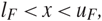
${L_{{G_1},F}}(x) \ge {L_{{G_2},F}}(x)$, ${l_F} \lt x \lt {u_F}$, for all absolutely continuous lifetime distribution functions F.(iii) The function
${{G_1^{ - 1}(u)} \over {G_2^{ - 1}(u)}}$, 0 < u < 1, is non-decreasing.




Moreover, a strict increase of the ratio in point (iii) is equivalent to the strict inequalities in (i) and (ii).
We also note that a (strict) increase of  ${{G_1^{ - 1}(u)} \over {G_2^{ - 1}(u)}}$ is equivalent to a (strict) decrease of its reciprocal.
Proof. (i) ⇒ (iii) The assumption asserts that
 $${{x{\kern 1pt} {f_0}(x)} \over {(G_1^{ - 1} \circ {F_0})(x)({g_1} \circ G_1^{ - 1} \circ {F_0})(x)}} \ge {{x{\kern 1pt} {f_0}(x)} \over {(G_2^{ - 1} \circ {F_0})(x)({g_2} \circ G_2^{ - 1} \circ {F_0})(x)}},\quad {l_{{F_0}}} \lt x \lt {u_{{F_0}}},$$
and is equivalent to
 $${1 \over {(G_1^{ - 1} \circ {F_0})(x)({g_1} \circ G_1^{ - 1} \circ {F_0})(x)}} \ge {1 \over {(G_2^{ - 1} \circ {F_0})(x)({g_2} \circ G_2^{ - 1} \circ {F_0})(x)}},\quad {l_{{F_0}}} \lt x \lt {u_{{F_0}}}.$$
Since F 0(x) takes on all the values in (0, 1) as x runs over  $({l_{{F_0}}},{u_{{F_0}}})$, we can also write
 $${1 \over {G_1^{ - 1}(u)({g_1} \circ G_1^{ - 1})(u)}} \ge {1 \over {G_2^{ - 1}(u)({g_2} \circ G_2^{ - 1})(u)}},\quad \quad 0 \lt u \lt 1,$$
which means that
 $${{\rm{d}} \over {{\rm{d}}u}}\ln G_1^{ - 1}(u) - {{\rm{d}} \over {{\rm{d}}u}}\ln G_2^{ - 1}(u) = {{\rm{d}} \over {{\rm{d}}u}}\ln {{G_1^{ - 1}(u)} \over {G_2^{ - 1}(u)}} \ge 0,\quad \quad 0 \lt u \lt 1.$$
This implies that the ratio  ${{G_1^{ - 1}(u)} \over {G_2^{ - 1}(u)}}$ is non-decreasing in (0, 1).
(iii) ⇒ (ii) The assumption implies (5). Plugging in F(x) = u and multiplying both fractions by xf (x), we get the desired claim.
The implication (ii) ⇒ (i) is obvious.
Careful analysis of the above reasoning allows us to conclude that a strict increase of  ${{G_1^{ - 1}(u)} \over {G_2^{ - 1}(u)}}$ is equivalent to the strict inequalities among the generalized ageing intensity functions in points (i) and (ii).
The following assertion was proven in [Reference Szymkowiak27, Proposition 1] under the restriction (lF, uF) = (0, +∞).
Proposition 2. For any absolutely continuous lifetime distribution function F, and for every lF < zx < uF,  ${L_{{W_\alpha },F}}(x)$ decreases in α ∊ ℝ.
Furthermore, the following lemma generalizes Lemma 1 of [27].
Lemma 1. For any lifetime distribution functions F, G, and H with positive density functions on their interval supports, we have
 $${L_{H,F}}(x) = {L_{H,G}}(({G^{ - 1}} \circ F)(x)){\kern 1pt} {L_{G,F}}(x).$$
Proof. Representing (H −1 ∘ F)(x) as (H −1 ∘ G ∘ G −1 ∘ F)(x), we get
 $$\matrix{
{{{d({H^{ - 1}} \circ F)(x)} \over {dx}} = {{d({H^{ - 1}} \circ G)(({G^{ - 1}} \circ F)(x))} \over {dx}}{{d({G^{ - 1}} \circ F)(x)} \over {dx}},} \cr
{{{({H^{ - 1}} \circ F)(x)} \over x} = {{({H^{ - 1}} \circ G)(({G^{ - 1}} \circ F)(x))} \over {({G^{ - 1}} \circ F)(x)}}{{({G^{ - 1}} \circ F)(x)} \over x}.} \cr } $$
Combining these formulae, we obtain
 $$\matrix{
{{L_{H,F}}\left( x \right)} & = & {{x \over {\left( {{H^{ - 1}}oF} \right)\left( x \right)}}{{{\rm{d}}\left( {{H^{ - 1}}oF} \right)\left( x \right)} \over {\left( {{H^{ - 1}}oF} \right)\left( x \right)}}} \cr
{} & = & {{{({G^{ - 1}}oF)(x){{\rm{d}} \over {{\rm{d}}x}}({H^{ - 1}}oG)(({G^{ - 1}}oF)(x))} \over {({H^{ - 1}}oG)(({G^{ - 1}}oF)(x)}}{{x{{{\rm{d}}({G^{ - 1}}oF)(x)} \over {({G^{ - 1}}oF)(x)}}} \over {}}} \cr
{} & = & {{L_{H,G}}(({G^{ - 1}}oF)(x)){L_{G,F}}(x).} \cr
} $$
Proposition 3. (i) If LG,F(x) ≤ a, lF < x < u F, and LH,G (x) ≤ b, lG < x < uG, then LH,F(x) ≤ ab, lF < x < uF.
(ii) If LG,F(x) ≤ a, lF < x < uF, then  ${L_{F,G}}(x) \ge {1 \over a}$, lG < x < uG.
Moreover, reversed inequalities in the assumptions of (i) and (ii) imply reversed inequalities in the respective conclusions.
Proof. (i) For every lF < x < uF we have (G −1 ∘ F)(x) ∊ (lG, uG), and therefore LH, G((G −1 ∘ F)(x)) ≤ b. Applying (6), we immediately get the claim.
(ii) We first note that LF,F(x) = 1 for arbitrary F and lF < x < uF. By (6) and the assumption, for every lG < y = (G −1 ∘ F)(x) < uG with lF < x < uF, we have
 $${L_{F,G}}(y) = {{{L_{F,F}}(x)} \over {{L_{G,F}}(x)}} \ge {1 \over a}.$$
The proofs of the reversed inequalities are analogous.
3. Characterization results
It is easy to show that for a fixed absolutely continuous lifetime distribution function G supported on an interval (lG, uG), a positive function r defined on (l, u) ⊂ (0, +∞)isthe G-generalized failure rate of a unique distribution function
 $$F(x) = G({l_G} + \int_l^x r(t){\kern 1pt} {\rm{d}}t)$$
with support (l, u). The necessary and sufficient condition for this representation is that
 $$\int_l^u r(t){\kern 1pt} {\rm{d}}t = {u_G} - {l_G}.$$
A continuous function R acting as an increasing transformation (l, u) onto (lG, uG)isthe G-generalized cumulative hazard function of a unique
 $$F(x) = (G \circ R)(x),\quad \quad l \lt x \lt u.$$
Obviously, there is also a unique characterization of F having the G-generalized average hazard rate H satisfying the conditions lH(l ) = lG, uH(u) = uG with an increasing function x ↦ xH(x) on (l, u). Reference [Reference Szymkowiak27] proved that for some α the Wα-generalized ageing intensity functions characterize single distributions, whereas for others parametric families of distributions are characterized. In the theorem presented below we show that this distinction appears for general G, and depends merely on the properties of the support of G. We also specify the conditions on functions L which enable them to be the G-generalized ageing intensity functions of some lifetime distributions for various types of supports of G.
Theorem 1. Let G denote here a distribution function with a positive density on its interval support (lG, uG) ⊂ (0, +∞). Assume that the function L :(l, u) ↦ (0, +∞), where 0 ≤ l < u ≤+∞, is locally integrable.
(i) In the case
(7)$$\int_a^b {{L(t)} \over t}{\kern 1pt} {\rm{d}}t \lt + \infty = \int_l^a {{L(t)} \over t}{\kern 1pt} {\rm{d}}t = \int_a^u {{L(t)} \over t}{\kern 1pt} {\rm{d}}t,\quad \quad l \lt a \lt b \lt u,$$
for every fixed distribution function G with the support (lG, uG) = (0, +∞), the function L is the G-generalized ageing intensity function for a family of absolutely continuous distribution functions supported on (l, u) and defined by the formula
(8)$${F_{G,L,k}}(x) = G(k\exp (\int_a^x {{L(t)} \over t}{\kern 1pt} {\rm{d}}t)),\quad \quad l \lt x \lt u,$$
with arbitrarily fixed l < a < u and every 0 < k < +∞.
(ii) In the case
(9)$$\int_l^a {{L(t)} \over t}{\kern 1pt} {\rm{d}}t \lt + \infty = \int_a^u {{L(t)} \over t}{\kern 1pt} {\rm{d}}t,\quad \quad l \lt a \lt u,$$
for every G supported on (lG, +∞) with some positive lG, the function L is the G-generalized ageing intensity function for a unique absolutely continuous distribution function supported on (l, u) defined as
(10)$${F_{G,L}}(x) = G({l_G}\exp (\int_l^x {{L(t)} \over t}{\kern 1pt} {\rm{d}}t)),\quad \quad l \lt x \lt u.$$
(iii) When
(11)$$\int_a^u {{L(t)} \over t}{\kern 1pt} {\rm{d}}t \lt + \infty = \int_l^a {{L(t)} \over t}{\kern 1pt} {\rm{d}}t,\quad \quad l \lt a \lt u,$$
and the support of G is (0, uG) for some 0 < uG < +∞, the function L is the G-generalized ageing intensity function for a unique absolutely continuous distribution function supported on (l, u) defined as
(12)$${F_{G,L}}(x) = G({u_G}\exp ( - \int_x^u {{L(t)} \over t}{\kern 1pt} {\rm{d}}t)),\quad \quad l \lt x \lt u.$$
(iv) Finally, in the case
(13)$$\int_l^u {{L(t)} \over t}{\kern 1pt} {\rm{d}}t \lt + \infty $$
the function L is the G-generalized ageing intensity function for a unique absolutely continuous distribution function supported on (l, u) which is defined by either of (10) and (12) for any G with support of the form
$$({l_G},{l_G}\exp (\int_l^u {{L(t)} \over t}{\rm{d}}t))$$
for some lG > 0.


Observe that under the assumption on the support of G in Theorem 1(iv),
 $${u_G}\exp ( - \int_x^u {{L(t)} \over t}{\kern 1pt} {\rm{d}}t) = {l_G}\exp (\int_l^x {{L(t)} \over t}{\kern 1pt} {\rm{d}}t),$$
and so (10) and (12) coincide.
Proof of Theorem 1. Suppose that L : (u, l) ↦ (0, +∞)is the G-generalized ageing intensity function of some absolutely continuous distribution function F with support (l, u). This means that the equation
 $${{L(x)} \over x} = {{{{\rm{d}} \over {{\rm{d}}x}}({G^{ - 1}} \circ F)(x)} \over {({G^{ - 1}} \circ F)(x)}}$$
holds for all l < x < u. For every a, x ∈ (l, u) we also have
 $$\int_a^x {{L(t)} \over t}{\kern 1pt} {\rm{d}}t = \int_a^x {{\rm{d}} \over {{\rm{d}}t}}[\ln ({G^{ - 1}} \circ F)(t)]{\rm{d}}t = \ln ({{({G^{ - 1}} \circ F)(x)} \over {({G^{ - 1}} \circ F)(a)}}).$$
Accordingly, we further obtain
 $$({G^{ - 1}} \circ F)(x) = ({G^{ - 1}} \circ F)(a)\exp (\int_a^x {{L(t)} \over t}{\kern 1pt} {\rm{d}}t),$$
and finally
 $$F(x) = G(({G^{ - 1}} \circ F)(a)\exp (\int_a^x {{L(t)} \over t}{\kern 1pt} {\rm{d}}t)).$$
Since 0 ≤ lG < (G −1 ∘ F)(a) < uG for each l < a < u, we have, for l < x < u,
 $$\matrix{
{{{\rm{d}} \over {{\rm{d}}x}}F(x){\kern 1pt} = {\kern 1pt} G(({G^{ - 1}} \circ F)(a)\exp (\int_a^x {{L(t)} \over t}{\kern 1pt} {\rm{d}}t))} \cr
{ \times ({G^{ - 1}} \circ F)(a)\exp (\int_a^x {{L(t)} \over t}{\kern 1pt} {\rm{d}}t){{L(x)} \over x} > 0.} \cr
} $$
We need to impose boundary conditions on (G −1 ∘ F)(a) so as to obtain F(l ) = 0 and F(u) = 1, which guarantee that F is absolutely continuous and supported on (l, u). The conditions depend on lG, uG, and accompanying assumptions on L.
(i) Suppose first that lG = 0 and uG =+∞. Then, by (14),
(16)$$\matrix{
{({G^{ - 1}} \circ F)(l) = {l_G} = 0 = ({G^{ - 1}} \circ F)(a){\kern 1pt} \exp ( - \int_l^a {{L(t)} \over t}{\kern 1pt} {\rm{d}}t),} \cr
{({G^{ - 1}} \circ F)(u) = {u_G} = + \infty = ({G^{ - 1}} \circ F)(a){\kern 1pt} \exp (\int_a^u {{L(t)} \over t}{\kern 1pt} {\rm{d}}t)} \cr
} $$
if L satisfies (7), independently of the particular value of (G −1 ∘ F)(a). It suffices then to notice that (G −1 ∘ F)(a)for l < a < u may take on any positive value k by the assumption on the supports of F and G, and the continuity of G −1 ∘ F. Then (15) with arbitrary 0 < k = (G −1 ∘ F)(a) < +∞ determines a distribution function F obeying the desired assumptions.
(ii) If lG > 0, then the relation
(17)$$({G^{ - 1}} \circ F)(l) = {l_G} = ({G^{ - 1}} \circ F)(a)\exp ( - \int_l^a {{L(t)} \over t}{\kern 1pt} {\rm{d}}t)$$
forces the finiteness of
$\int_l^a {{L(t)} \over t}{\kern 1pt} {\rm{d}}t$ for any l < a < u, and allows us to determine(18)$$({G^{ - 1}} \circ F)(a) = {l_G}\exp (\int_l^a {{L(t)} \over t}{\kern 1pt} {\rm{d}}t).$$
Similarly, for uG < +∞ we conclude that
$\int_a^u {{L(t)} \over t} {\rm{d}}t < + \infty $ for all l < a < u, and determine$$({G^{ - 1}} \circ F)(a) = {u_G}\exp ( - \int_a^u {{L(t)} \over t}{\kern 1pt} {\rm{d}}t).$$
Assume now that lG > 0 and uG =+∞. Equations (16) and (17) imply the necessity of assumptions (9). Moreover, plugging (18)into(15) we obtain (10).
(iii) For lG = 0 and uG < +∞, in much the same way we deduce that assumptions (11) are necessary, and the unique F with G-generalized ageing intensity L has the representation (12).
(iv) If 0 < lG < uG < +∞, both representations (10) and (10) are valid. They are identical for all l < x < u if assumption (7) is satisfied.


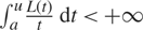

The integral conditions (7), (9), (11), and (13) combined with respective restrictions on the support end-points lG and uG are also necessary for the G-generalized ageing intensity functions of any distribution function F.
Corollary 1. Let F and G be distribution functions with positive density functions on respective support intervals (lF, uF) and (lG, uG), both contained in (0, +∞). Then LG,F is a positive function on (lF, uF) and satisfies (7), (9), (11), and (13) when lG = 0 < uG =+∞, 0 < lG < uG =+∞,lG = 0 < uG < +∞, and 0 < lG < uG < +∞, respectively.
Proof. The conclusions follow from the equations
 $$\matrix{
{{l_G} = ({G^{ - 1}} \circ F)(a)\exp ( - \int_{{l_F}}^a {{{L_{G,F}}(t)} \over t}{\kern 1pt} {\rm{d}}t),} \cr
{{u_G} = ({G^{ - 1}} \circ F)(a)\exp (\int_a^{{u_F}} {{{L_{G,F}}(t)} \over t}{\kern 1pt} {\rm{d}}t),} \cr
} $$
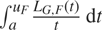
where 0 < (G −1 ∘ F)(a) < +∞ for arbitrarily chosen lF < a < uF, established in the proof of Theorem 1. The relations lG = 0 and lG > 0 imply that 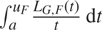 $\int_{{l_F}}^a {{{L_{G,F}}(t)} \over t}{\kern 1pt} {\rm{d}}t$ is respectively equal to and less than +∞. Similarly, uG < +∞ and uG =+∞ are equivalent to the respective finiteness and infiniteness of
 $\int_a^{{u_F}} {{{L_{G,F}}(t)} \over t}{\kern 1pt} {\rm{d}}t.$$
Suppose that LG,F is the G-generalized ageing intensity of some F, and we are interested in determining all the other distribution functions which have the same G-generalized ageing intensity. If lG = 0 and uG =+∞ then we can write
 $$\int_a^x {{{L_{G,F}}(t)} \over t}{\kern 1pt} {\rm{d}}t = \ln ({G^{ - 1}} \circ F)(x) - \ln ({G^{ - 1}} \circ F)(a).$$
This takes on the simplest form when the dependence on a is hidden, i.e. for a = (F −1 ∘ G)(1), for which the last terms on the right-hand side of the above equation vanish. Then we obtain
 $${F_{G,{L_{G,F}},k}}(x) = G(k{\kern 1pt} ({G^{ - 1}} \circ F)(x))\quad {\rm{for}}\;\;{l_F} \lt x \lt {u_F}\;\;{\rm{and}}\;\;k > 0.$$
Observe that if k = 1 in formula (19), we recover the baseline distribution function. If we take G = F, we have
 $${{F}_{F,{{L}_{F,F}},k}}(x)=F(kx)\quad \text{for}\ \ {{l}_{F}}\text{ }x\text{ }{{u}_{F}}\ \ \text{and}\ \ k>0,$$
which means that all the distribution functions sharing the F-generalized ageing intensity with F are scale transformations of the original F. If either lG > 0 or uG < +∞, and LG,F satisfies the respective integrability conditions of Theorem 1 (ii)–(iv), then the only distribution function with G-generalized ageing intensity LG,F is F itself.
It is clear that for given absolutely continuous life distribution functions F and G we can uniquely determine the G-generalized ageing intensity LG, F of F. Theorem 1 describes possible distribution functions F which have G-generalized ageing intensity L for fixed G. A natural question is for which G a given function L is the G-generalized ageing intensity of a fixed F. It happens that such a G is uniquely characterized up to the scale parameter.
Proposition 4. Let F be a lifetime distribution function with a positive density function on an interval (lF, uF) ⊂ (0, +∞). Let L : (lF, uF) ↦ (0, +∞) satisfy 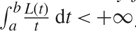 $\int_a^b {{L(t)} \over t}{\kern 1pt} {\rm{d}}t \lt + \infty $ for all lF < a < b < uF. The function L is the G-generalized ageing intensity function of F for some G if and only if L is the Gk-generalized ageing intensity function of F for
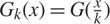 ${G_k}(x) = G({x \over k})$ with arbitrary 0 < k < +∞.
Proof. Note that 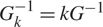 $G_k^{ - 1} = k{G^{ - 1}}$$. Therefore
 $${L_{{G_k},F}}(x) = {{kx{\kern 1pt} {{\rm{d}} \over {{\rm{d}}x}}({G^{ - 1}} \circ F)(x)} \over {(k{\kern 1pt} {G^{ - 1}} \circ F)(x)}} = {L_{G,F}}(x) = L(x),\quad \quad {l_F} \lt x \lt {u_F}.$$
Suppose now that some L is both the G- and H-generalized ageing intensity of F, i.e.
 $${{\rm{d}} \over {{\rm{d}}x}}[\ln ({G^{ - 1}} \circ F)(x) - \ln ({H^{ - 1}} \circ F)(x)] = 0,\quad \quad {l_F} \lt x \lt {u_F}.$$
This implies that (G −1 ∘ F)(x) = (kH −1 ∘ F)(x) for some positive k and all lF < x < uF. As x varies over (lF, uF), F(x) takes on all the values in (0, 1). We have G −1(u) = kH −1(u), 0 < u < 1, and 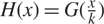 $H(x) = G({x \over k})$ in consequence.
Clearly, if one of conditions (9), (11), and (13) holds, then the support of G is a proper subset of (0, +∞), and the supports of the various Gk differ. The above considerations imply that Fi have identical Gi-generalized ageing intensity functions, i = 1, 2, if and only if the compositions  $G_1^{ - 1} \circ {F_1}$ and
 $G_2^{ - 1} \circ {F_2}$ are proportional.
It is also possible to determine various pairs Gi, Li, i = 1, 2, which uniquely characterize a fixed F in Theorem 1 (ii)–(iv). Suppose, e.g., that Gi are supported on (li, +∞), li > 0, whereas Li are positive on (l, u) ⊂ (0, +∞) and satisfy (9). Suppose that
 $$F(x) = {G_1}({l_1}\exp (\int_l^x {{{L_1}(t)} \over t}{\kern 1pt} {\rm{d}}t)) = {G_2}({l_2}\exp (\int_l^x {{{L_2}(t)} \over t}{\kern 1pt} {\rm{d}}t)),\quad \quad l \lt x \lt u.$$
The functions  ${\xi _i}(x) = \exp (\int_l^x {{{L_i}(t)} \over t}{\kern 1pt} {\rm{d}}t)$, i = 1, 2, provide increasing transformations of (l, u) onto (1, +∞). The relations (21) imply that
 $$(G_1^{ - 1} \circ {G_2})(x) = ({l_1}{\kern 1pt} {\xi _1} \circ \xi _2^{ - 1})({x \over {{l_2}}}).$$
This formula looks especially nice when l 1 = l 2 = 1. Conditions that different pairs Gi, Li, i = 1, 2, characterize the same family of distribution functions {Fk :0 < k < +∞} of Theorem 1(i) are more restrictive.
Proposition 5. For i = 1 and i = 2 the function Li : (l, u) ↦ (0 +∞) is the Gi-generalized ageing intensity for the family of distribution functions {Fk, 0 < k < +∞} if and only if there exist a, b > 0 such that
 $${L_2}(x) = {1 \over a}{\kern 1pt} {L_1}(x),\quad \quad \;l \lt x \lt u,$$
 $${G_2}(x) = {G_1}(b{x^a}),\quad \quad 0 \lt x \lt + \infty .$$
Proof. (⇒) Under the assumptions, Gi, i = 1, 2, have positive density functions on (0, +∞). Moreover, we have
 $${F_k}(x) = {G_1}((k{\kern 1pt} G_1^{ - 1} \circ F)(x)) = {G_2}((\eta (k){\kern 1pt} G_2^{ - 1} \circ F)(x))$$
(cf. (19)) for all l < x < u and 0 < k < +∞, where F is a fixed representative of the family {Fk:0 < k < +∞}, and η :(0, +∞) ↦ (0, +∞) is a bijection. The function η is introduced here because we cannot guarantee that using different pairs Li and Gi provides a common parametrization of {Fk:0 < k < +∞}. At the moment, we cannot be assured that η is either continuous or monotonic.
Denote  $G_1^{ - 1} \circ {G_2}$ as ζ. This is a continuous increasing function acting from (0, +∞) onto (0, +∞). We obviously have G 2(x) = (G 1 ∘ ζ )(x) and
 $G_2^{ - 1}(u) = ({\zeta ^{ - 1}} \circ G_1^{ - 1})(u)$. Using (24) and the above notation, we can write
 $${G_1}((k{\kern 1pt} G_1^{ - 1} \circ F)(x)) = {G_1}(\zeta ((\eta (k){\kern 1pt} {\zeta ^{ - 1}} \circ G_1^{ - 1} \circ F)(x)))$$
for all l < x < u and 0 < k <+∞. All possible values of 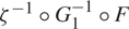 ${\zeta ^{ - 1}} \circ G_1^{ - 1} \circ F$ constitute the positive half-axis (0, +∞). The inverse function η −1 transforms (0, +∞) onto (0, +∞). Relation (25) forces that
 $${\eta ^{ - 1}}(y)\zeta (z) = \zeta (yz)$$
for all  $0 \lt y = \eta (k) \lt + \infty $,
 $z = ({\zeta ^{ - 1}} \circ G_1^{ - 1} \circ F)(x) \lt + \infty $. This in particular means that η −1( y)ζ (z) = η −1(z)ζ ( y) for any 0 < y, z < +∞. Writing
 $${{\zeta (y)} \over {{\eta ^{ - 1}}(y)}} = {{\zeta (z)} \over {{\eta ^{ - 1}}(z)}},$$
fixing z, and letting y vary, we deduce that 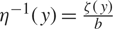 ${\eta ^{ - 1}}(y) = {{\zeta (y)} \over b}$ for some constant b which is positive by the positiveness of both η −1 and ζ. Plugging it into (26) we obtain
 $$\zeta (y)\zeta (z) = b{\kern 1pt} \zeta (yz),\quad \quad y,z > 0.$$
The function  ${\zeta _b}(y) = {{\zeta (y)} \over b}$ satisfies the multiplicative Cauchy equation
 $${\zeta _b}(y){\zeta _b}(z) = {\zeta _b}(yz),\quad \quad y,z > 0,$$
and is continuous by definition. Therefore ζb( y) = ya for some a > 0, because ζb is increasing as well. This implies that  $\zeta (x) = (G_1^{ - 1} \circ {G_2})(x) = b{x^a}$, which proves (23), whereas
 $\eta (k) = {k^{{1 \over a}}}$. Since, moreover,
 $$(G_2^{ - 1} \circ F)(x) = [({1 \over b}G_1^{ - 1} \circ F)(x{)]^{{1 \over a}}}$$, we immediately get (22).
(⇐) The implication here is obvious.
4. Characterizations by elasticity functions
We say that φ : [0, 1] ↦ [0, 1] is a distortion function if it is non-decreasing and φ(0) = 0, φ(1) = 1. The notion was primarily introduced in [Reference Denneberg10] in risk theory (see, e.g., [24] for further developments). The usefulness of the distortion function in reliability theory was presented in [Reference Navarro, Del Aguila, Sordo and Suárez-Llorens18, Reference Navarro, Del Aguila, Sordo and Suárez-Llorens19]. For a given differentiable function ξ :(lξ, uξ) ↦ (0, +∞) with (lξ, uξ ) ⊂ (0, +∞), we define the elasticity of ξ as
 $${E_\xi }(x) = {{x{\kern 1pt} {{\rm{d}} \over {{\rm{d}}x}}\xi (x)} \over {\xi (x)}},\quad \quad {l_\xi } \lt x \lt {u_\xi }.$$
Elasticity is one of the most important economic concepts (see, e.g., [Reference Case and Fair6, Reference Chiang and Wainwright9, Reference Marshall16, Reference Navarro, Del Aguila, Sordo and Suárez-Llorens18, Reference Veres-Ferrer and Pavía29]). It measures how one economic variable (demand, say) reacts on the change of another one (supply, say). If ξ(x) is a demand function of supply x, and |Eξ (x)| > 1, we claim that the demand is elastic, which means that a small change in supply implies a significant change in demand. On the contrary, for |Eξ (x)| < 1 the demand is inelastic, i.e. a significant change of supply does not affect the demand much.
Proposition 6. Let φ be a fixed distortion function with a positive derivative on (0, 1). The function E :(l, u) ↦ (0, +∞) satisfying the conditions
 $$\int_a^u {{E(t)} \over t}{\kern 1pt} {\rm{d}}t \lt + \infty = \int_l^a {{E(t)} \over t}{\kern 1pt} {\rm{d}}t$$
for all l < a < u is the elasticity of the composition φ ∘ F for a unique absolutely continuous distribution function F supported on (l, u) and defined by the formula
 $$F(x) = {\varphi ^{ - 1}}(\exp ( - \int_x^u {{E(t)} \over t}{\kern 1pt} {\rm{d}}t)),\quad \quad l \lt x \lt u.$$
Proof. The inverse φ −1 of φ is an absolutely continuous distribution function on  $({l_{{\varphi ^{ - 1}}}},{u_{{\varphi ^{ - 1}}}}) = (0,1)$ with a positive density there. The function E satisfies the assumptions of Theorem 1(iii). This implies that this is the φ −1-generalized ageing intensity function
 $$E(x) = {{x{\kern 1pt} {{\rm{d}} \over {{\rm{d}}x}}(\varphi \circ F)(x)} \over {(\varphi \circ F)(x)}} = {L_{{\varphi ^{ - 1}},F}}(x)$$
of a unique distribution function satisfying (28).
Although the above proposition was formulated for elasticity functions defined on general intervals (lξ, uξ ), it is natural to assume in practice that lξ = 0. In particular, we do so in the applications presented below. Under the assumption, the equality in (28) is attained when E is separated from zero for small arguments. This means, for instance, that the demand does not vanish as the supply decreases to zero. This is a natural prerequisite in practice. If, moreover, uξ < +∞ (the supply has a natural upper bound) then every bounded demand elasticity function of supply with a positive infimum satisfies both the relations in (28). For uξ = + ∞,(28)implies that E decreases to 0 at a sufficiently fast rate. This happens in practice as well, because in the case of great supply, small supply variations do not visibly affect the demand. A simple and natural elasticity function satisfying (28)on (0, +∞) is a decreasing exponential function.
Reference [Reference Szymkowiak27] proved that the elasticity of the distribution of the minimum of n independent and identically distributed (i.i.d.) random variables uniquely characterizes the parent distribution function. Taking  $\varphi = {\varphi _{k:n}}(x) = \sum\nolimits_{i = k}^n n\matrix{
{} \cr
i \cr
} {x^i}{(1 - x)^{n - i}}$ and applying Proposition 1, we generalize the statement to arbitrary-order statistics. Moreover, every function E satisfying (27) may represent the elasticity
 $$E(x) = {{x{{[1 - F(x)]}^{k - 1}}{{{{[ - k\ln (1 - F(x))]}^{n - 1}}} \over {(n - 1)!}}} \over {1 - {{[1 - F(x)]}^k}\sum\limits_{i = 0}^{n - 1} {{{{[ - k\ln (1 - F(x))]}^i}} \over {i!}}}}$$
of the distribution function of the nth value of the kth record, which uniquely determines the parent distribution function F for any positive integer n and k. More generally, the elasticity of the distribution function of the rth generalized-order statistics for arbitrarily fixed parameters λ 1,...,λr > 0 characterizes the baseline distribution (we do not recall the distortion function formula which is just the distribution function of the respective generalized order statistics in the uniform case, due to its complexity).
On the other hand, if we take a system with a given structure, and given the resulting Samaniego signatures = (s 1,..., sn) composed of n items with i.i.d. lifetimes, then knowledge of the system lifetime distribution elasticity
 $${E_{\bf{s}}}(x) = {{nx\sum\limits_{i = 1}^n {s_i}n - 1\matrix{
{} \cr
{i - 1} \cr
} {F^{i - 1}}(x)[1 - F(x{{)]}^{n - i}}} \over {\sum\limits_{i = 1}^n (\sum\limits_{j = i}^n {s_j})n\matrix{
{} \cr
i \cr
} {F^i}(x)[1 - F(x{{)]}^{n - i}}}}$$
allows us to recover the component lifetime distribution function F. The same conclusion can be drawn if we assume that the components operate in the failure-dependent proportional hazard regime, which implies that the component lifetimes are exchangeable, and their order statistics follow the assumptions of the generalized-order statistics model.
The problem is, though, that quite often the method of construction presented in Proposition 6 does not provide an analytic representation of F. One reason is that the indefinite integral 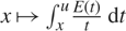 $x \mapsto \int_x^u {{E(t)} \over t}{\kern 1pt} {\rm{d}}t$ does not have an analytic form. The other is that the inverse φ −1 of the distortion function cannot be represented by a closed formula. Among the examples mentioned above, only the distortions φ 1:n and φn :n representing the sample extremes have tractable inverses
 $\varphi _{1:n}^{ - 1}(x) = 1 - {(1 - x)^{{1 \over n}}}$ and
 $\varphi _{n:n}^{ - 1}(x) = {x^{{1 \over n}}}$, 0 < x < 1, respectively. Elasticity functions E satisfying Proposition 6 of the compositions φi :n ∘ F, i = 1 and n, uniquely characterize the distribution functions
 $${F_{1:n,E}}(x) = 1 - {[1 - \exp ( - \int_x^u {{E(t)} \over t}{\kern 1pt} {\rm{d}}t)]^{{1 \over n}}},$$
 $${F_{n:n,E}}(x) = \exp ( - {1 \over n}\int_x^u {{E(t)} \over t}{\kern 1pt} {\rm{d}}t),\quad \quad \quad \quad \quad \quad l \lt x \lt u,$$
respectively. In particular, if E(x) = bx −a,0 < x < +∞,for some a, b > 0, then
 $$\matrix{
{{F_{1:n,E}}(x) = 1 - {{[1 - \exp ( - {b \over a}{\kern 1pt} {x^{ - a}})]}^{{1 \over n}}},} \cr
{{F_{n:n,E}}(x) = \exp ( - {b \over {na}}{\kern 1pt} {x^{ - a}}),\quad \quad \quad \quad \quad \quad \quad \quad 0 \lt x \lt + \infty ,} \cr
}$$
respectively. Much more complicated but still possible is characterization by the median of sample of size 3 for which φ 2:3(x) = 3x 2 − 2x 3,0 < x < 1. The problem consists in finding solutions to the cubic parametric equations
 $$2{y^3} - 3{y^2} + x = 0,\quad \quad 0 \lt x \lt 1,$$
belonging to the interval (0, 1). We easily conclude that each equation has three real solutions, and using the classical Viète method we determine solutions contained in (0, 1) which define the inverse function
 $$\varphi _{2:3}^{ - 1}(x) = {1 \over 2} - \cos ({1 \over 3}[\pi + \arccos (1 - 2x)]),\quad \quad 0 \lt x \lt 1,$$
and in consequence
 $${F_{2:3,E}}(x) = \varphi _{2:3}^{ - 1}(\exp ( - \int_x^u {{E(t)} \over t}{\kern 1pt} {\rm{d}}t)),\quad \quad l \lt x \lt u.$$
Formulae (29) and (30) with n = 3 and (32) with (31) represent characterizations by distortions of k-out-of-3 systems with k = 1, 3, and 2, respectively. There are only two other coherent systems with three components with structure functions
 $${\phi _1}({x_1},{x_2},{x_3}) = \max \{ {x_1},\min \{ {x_2},{x_3}\} \} ,$$
 $${\phi _2}({x_1},{x_2},{x_3}) = \min \{ {x_1},\max \{ {x_2},{x_3}\} \} ,$$
and respective signatures 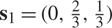 ${{\bf{s}}_1} = (0,{2 \over 3},{1 \over 3})$ and
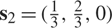 ${{\bf{s}}_2} = ({1 \over 3},{2 \over 3},0)$. The first one generates the distortion function φ 1(x) = 2x 2 − x 3, which has inverse
 $$\varphi _1^{ - 1}(x) = {2 \over 3} - {4 \over 3}\cos ({1 \over 3}[\pi + \arccos {{16 - 27x} \over {16}}]),\quad \quad 0 \lt x \lt 1.$$
Since φ 2(x) = 1 − φ 1 (1 − x), we also have  $\varphi _2^{ - 1}(x) = 1 - \varphi _1^{ - 1}(1 - x)$, 0 < x < 1. The distortion functions of systems (33) and (34) together with the elasticity function E satisfying the assumptions of Proposition 6 characterize the distribution functions
 $$\begin{align}
& {{F}_{1,E}}(x)=\frac{2}{3}-\frac{4}{3}\cos \,\left( \frac{1}{3}[\pi +\arccos \,\,\left( 1-\frac{27}{16}\operatorname{ex} \right.p \right.\left. \left. (-\int_{x}^{u}{\frac{E(t)}{t}}\text{ d}t \right) \right)]), \\
& {{F}_{2,E}}(x)=\frac{2}{3}-\frac{4}{3}\cos \,\left. \left( \frac{1}{3}[\pi +\arccos \,\left( \frac{27}{16}\operatorname{e} \right.x \right.\left. p\left( -\int_{x}^{u}{\frac{E(t)}{t}}\text{ d}t) \right.-\frac{11}{16} \right] \right), \\
\end{align}\$$
respectively, for all arguments from the domain of E.
5. Examples of characterization through G-generalized ageing intensity
We assume that absolutely continuous lifetime distribution functions F and G have positive density functions f and g, respectively, on some interval supports (lF, uF) and (lG, uG), respectively, contained in (0, +∞). We will determine distribution functions which have G-generalized ageing intensities LG,F identical with those of the selected lifetime distribution function F for various G.
Example 1. Let F(x) = Fλ(x) = 1 − exp(−λx)for x ∊ (0, +∞) be the exponential distribution function with fixed scale parameter λ> 0.
1. Suppose that G(x) = Gβ,λ (x) = 1 − exp(−βxλ) for x ∊ (0, +∞) is the two-parameter Weibull distribution function (see [Reference Marshall and Olkin17]) with given shape parameter λ > 0 and scale parameter
${\beta ^{{1 \over \gamma }}} > 0$. Then lG = 0 and uG =+∞ for any λ and β. Obviously, for λ = 1 it is the exponential distribution with scale parameter β > 0.For general λ and β we have
$$(G{{_{\beta ,\gamma }^{-1}}^{{}^\circ }}{{F}_{\lambda }})(x)={{(\frac{\lambda }{\beta }x)}^{\frac{1}{\gamma }}}$$ and the respective ageing intensity$${L_{{G_{\beta ,\gamma }},{F_\lambda }}}(x) = {1 \over \gamma }\;\;for\;\;x \in (0, + \infty ).$$
The indefinite integral
$\int {{L(x)} \over x}{\kern 1pt} {\rm{d}}x = {1 \over \gamma }\ln x + C$, which implies that L satisfies (7), and by (8) it characterizes the scale family of exponential distribution functions(35)$${F_{k'}}(x) = 1 - \exp ( - k'x),\quad \quad 0 \lt x \lt + \infty ,$$
for k ′ = kλ λ ∊ (0, +∞) (cf.(20)).
This illustrates the results of Proposition 4 asserting that L does not depend on the scale parameter of distribution G.The G-generalized ageing intensities
${L_{{G_{\beta ,\gamma }},{F_\lambda }}}$ and ${L_{{G_{\beta ,1}},{F_\lambda }}}$ for Gβ,λ and Gβ, 1, being respectively Weibull and the exponential distributions, characterize the same scaled exponential family (35). This illustrates the results of Proposition 5.2. Assume now that G(x) = Gβ,λ,θ (x) = 1 − exp (−β(x − θ)λ) for x ∊ (θ, +∞) is the three-parameter Weibull distribution function (see [Reference Weibull30]) with shape parameter λ > 0, parameter β > 0, and location parameter θ > 0. This differs from the previous case by translating the distribution support from (0, +∞) to (θ, +∞). We have
$$(G_{\beta ,\gamma ,\theta }^{ - 1}t^\circ {F_\lambda })(x) = {({\lambda \over \beta }x)^{{1 \over \gamma }}} + \theta $$ and ultimately(36)$${L_{{G_{\beta ,\gamma ,\theta }},{F_\lambda }}}(x) = {{{1 \over \gamma }{{({\lambda \over \beta }x)}^{{1 \over \gamma }}}} \over {{{({\lambda \over \beta }x)}^{{1 \over \gamma }}} + \theta }}\quad for\;x \in (0, + \infty ).$$
The indefinite integral
$\int {{L(x)} \over x}{\kern 1pt} {\rm{d}}x = \ln (({\lambda \over \beta }x{)^{{1 \over \gamma }}} + \theta ) + C$ is finite at 0 and has the limit +∞ at +∞. Therefore conditions (9) of Theorem 1(ii) are satisfied.Due to (10), the only distribution function with Gβ,λ,θ -generalized ageing intensity (36) is
$${F_{{G_{\beta ,\gamma ,\theta }},{L_{{G_{\beta ,\gamma ,\theta }},{F_\lambda }}}}}(x) = {G_{\beta ,\gamma ,\theta }}(({\lambda \over \beta }{\kern 1pt} x{)^{{1 \over \gamma }}} + \theta ) = {F_\lambda }(x).$$
We notice that shifting the original distribution function Gβ,λ starting from 0 by an arbitrary amount θ to the right radically changes the characterization results.
3. For positive scale parameter β and shape parameters λ and α, let the distribution
$${G_{\alpha ,\beta ,\gamma }}(x) = 1 - {(1 + \beta {x^\alpha })^{ - \gamma }},\quad \quad 0 \lt x \lt + \infty ,$$
be a member of the power Lomax family (see [Reference Rady, Hassanein and Elhaddad22]). Note that for α = 1 we get the standard Lomax distribution (see [Reference Johnson, Kotz and Balakrishnan13]). We can easily check that
$$(G_{\alpha ,\beta ,\gamma }^{ - 1} \circ {F_\lambda })(x) = ({1 \over \beta }(\exp ({\lambda \over \gamma }x) - {1))^{{1 \over \alpha }}}.$$
The respective ageing intensity
(37)$${L_{{G_{\alpha ,\beta ,\gamma }},{F_\lambda }}}(x) = {1 \over \alpha }{\lambda \over \gamma }x{\kern 1pt} {{\exp ({\lambda \over \gamma }x)} \over {\exp ({\lambda \over \gamma }x) - 1}},\quad \quad 0 \lt x \lt + \infty ,$$
does not depend on the scale parameter, as claimed in Proposition 4. The indefinite integral
$$\int {{{L_{{G_{\alpha ,\beta ,\gamma }},{F_\lambda }}}(x)} \over x}{\kern 1pt} {\rm{d}}x = {1 \over \alpha }\ln (\exp ({\lambda \over \gamma }x) - 1) + C$$
tends to −∞ and +∞ as x approaches 0 and +∞, respectively. Accordingly, (37) satisfies (7).
Applying (8), we check that (37) characterizes the family of distribution functions
$${F_{k',\gamma ,\lambda }} = 1 - {[k'\exp ({\lambda \over \gamma }x) - k' + 1]^{ - \gamma }},\quad \quad 0 \lt x \lt + \infty ,\;0 \lt k \lt + \infty ,$$
for k ′ = kα ∊ (0, +∞).
4. Take now the Pareto I distribution function (see [Reference Johnson, Kotz and Balakrishnan13])
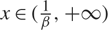
$G(x) = {\tilde G_{\beta ,\gamma }}(x) = 1 - {(\beta {\kern 1pt} x)^{ - \gamma }}$ for $x \in ({1 \over \beta }, + \infty )$ with shape parameter λ > 0 and scale parameter β > 0. Then ${l_{\tilde G}} = {1 \over \beta } > 0$ and ${u_{\tilde G}} = + \infty $.By simple calculation we obtain
$(\tilde G_{\beta ,\gamma }^{ - 1} \circ {F_\lambda })(x) = {1 \over \beta }\exp ({\lambda \over \gamma }x)$. We also check that the respective generalized ageing intensity(38)$${L_{{{\tilde G}_{\beta ,\gamma }},{F_\lambda }}}(x) = {\lambda \over \gamma }{\kern 1pt} x\quad for\;x \in (0, + \infty )$$
does not depend on β, and the indefinite integral
$\int {{L(x)} \over x}{\kern 1pt} {\rm{d}}x = {\lambda \over \gamma }x + C$ satisfies (9).By Theorem 1(ii) the only distribution function with
${\tilde G_{\beta ,\gamma }}$-generalized ageing intensity function (38) is the original exponential distribution function Fλ itself. Note that ${\tilde G_{\beta ,\gamma }}$ is just the G 1, β, λ of the previous point and the translation modified argument $x - {1 \over \beta }$. This explains the differences between the results of points 1 and 2 and those of 3 and 4.5. Suppose further that
$G(x) = {G_{\beta ,\gamma ,\theta ,\vartheta }}(x) = 1 - \exp [ - \beta {({{x - \theta } \over {\vartheta - x}})^\gamma }]$ with x ∊ (θ, ϑ) is an arbitrary member of the four-parameter class of distribution functions that arises from the five-parameter family of Weibull distribution functions (see [Reference Phani20]) by equating two shape parameters, λ = γ > 0. The location parameters satisfy 0 < lG = θ < uG = ϑ < + ∞, and β is positive.We get
(39)$$(G_{\beta ,\gamma ,\theta ,\vartheta }^{ - 1} \circ {F_\lambda })(x) = {{\vartheta {{({\lambda \over \beta }x)}^{{1 \over \gamma }}} + \theta } \over {{{({\lambda \over \beta }x)}^{{1 \over \gamma }}} + 1}}.$$
The respective ageing intensity
(40)$${L_{{G_{\beta ,\gamma ,\theta ,\vartheta }},{F_\lambda }}}(x) = {{{1 \over \gamma }{{({\lambda \over \beta }x)}^{{1 \over \gamma }}}(\vartheta - \theta )} \over {(\vartheta {{({\lambda \over \beta }x)}^{{1 \over \gamma }}} + \theta )(1 + {{({\lambda \over \beta }x)}^{{1 \over \gamma }}})}}\quad for\;x \in (0, + \infty ),$$
and the indefinite integral
(41)$$\int {{L(x)} \over x}{\kern 1pt} {\rm{d}}x = \ln \left( {{{\vartheta {\kern 1pt} {{({\lambda \over \beta }x)}^{{1 \over \gamma }}} + \theta } \over {{{({\lambda \over \beta }x)}^{{1 \over \gamma }}} + 1}}} \right) + C.$$
It follows that
$$\int_0^{ + \infty } {{{L_{{G_{\beta ,\gamma ,\theta ,\vartheta }},{F_\lambda }}}(x)} \over x}{\kern 1pt} {\rm{d}}x = \ln \vartheta - \ln \theta ,$$
and condition (13) is satisfied. Then (10) and (12) have the identical representation
(42)$$\matrix{
{{G_{\beta ,\gamma ,\theta ,\vartheta }}(\theta \exp (\int_0^x {{{L_{{G_{\beta ,\gamma ,\theta ,\vartheta }},{F_\lambda }}}(x)} \over x}{\kern 1pt} {\rm{d}}x))} \cr
{\quad = {G_{\beta ,\gamma ,\theta ,\vartheta }}(\vartheta \exp ( - \int_x^{ + \infty } {{{L_{{G_{\beta ,\gamma ,\theta ,\vartheta }},{F_\lambda }}}(x)} \over x}{\kern 1pt} {\rm{d}}x))} \cr
{\quad = {G_{\beta ,\gamma ,\theta ,\vartheta }}\left( {{{\vartheta {\kern 1pt} {{({\lambda \over \beta }x)}^{{1 \over \gamma }}} + \theta } \over {{{({\lambda \over \beta }x)}^{{1 \over \gamma }}} + 1}}} \right),} \cr
} $$
which ultimately simplifies to Fλ(x), as claimed in Theorem 1(iv). Observe that for θ = 0wehave
$$\int_a^{ + \infty } {{{L_{{G_{\beta ,\gamma ,\theta ,\vartheta }},{F_\lambda }}}(t)} \over t}{\kern 1pt} {\rm{d}}t = \ln \vartheta - \ln {\kern 1pt} {{\vartheta {\kern 1pt} {{({\lambda \over \beta }x)}^{{1 \over \gamma }}}} \over {{{({\lambda \over \beta }x)}^{{1 \over \gamma }}} + 1}} \lt + \infty = \int_0^a {{{L_{{G_{\beta ,\gamma ,\theta ,\vartheta }},{F_\lambda }}}(t)} \over t}{\kern 1pt} {\rm{d}}t,$$
i.e. (9) holds. Then all of (39)–(41), and the latter equality in (42) with θ = 0, are still valid (the first expression does not make sense then), and a single Fλ is characterized again by Theorem 1(iii).
6. Finally, suppose that
$G(x) = {G_{\alpha ,\beta ,\gamma ,\theta }}(x) = 1 - {[1 + {(\beta (x - \theta ))^{{1 \over \alpha }}}]^{ - \gamma }}$ for x ∊ (θ, +∞) is the Pareto IV distribution function (see [Reference Johnson, Kotz and Balakrishnan13]) with shape parameters α, λ > 0, parameter β> 0, and location parameter θ. Then lG = θ > 0 and uG =+∞.Moreover, we have that
$$(G_{\alpha ,\beta ,\gamma ,\theta }^{-1}{}^\circ {{F}_{\lambda }})(x)=\frac{1}{\beta }{{(\exp (\frac{\lambda }{\gamma }x)-1)}^{\alpha }}+\theta $$. The respective ageing intensity is(43)$${L_{{G_{\alpha ,\beta ,\gamma ,\theta }},{F_\lambda }}}(x) = {{{\alpha \over \beta }{\lambda \over \gamma }{\kern 1pt} x\exp ({\lambda \over \gamma }{\kern 1pt} x)} \over {{1 \over \beta }{{(\exp ({\lambda \over \gamma }{\kern 1pt} x) - 1)}^\alpha } + \theta }}\quad for\;x \in (0, + \infty ),$$
and the indefinite integral
$\int {{L(x)} \over x}{\kern 1pt} {\rm{d}}x = \ln ({1 \over \beta }{(\exp ({\lambda \over \gamma }{\kern 1pt} x) - 1)^\alpha } + \theta ) + C$ satisfies (9).By Theorem 1(ii), the only distribution function with Gα,β,λ,θ -generalized ageing intensity function (43) is the exponential distribution function itself.
















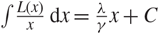









 $$L(x) = \sum\limits_{i = j}^k {b_i}{x^{{a_i}}},\quad l \lt x \lt u,$$
for l = 0, u = + ∞, some ordered aj < ⋯ < a 0 = 0 < ⋯ < ak, j ≤ 0 < k, and bi
= 0 for all i = j,..., k except for possibly b 0. Suppose that it satisfies the assumptions of Theorem 1(i). Taking all the bi positive we assert that so is L on the whole (0, +∞), but by no means is this a necessary condition. The assumption  $\int_0^a {{L(t)} \over t}{\kern 1pt} {\rm{d}}t = + \infty for\,\, some\,\, a > 0$ implies that bj > 0. Similarly,
 $\int_a^{ + \infty } {{L(t)} \over t}{\kern 1pt} {\rm{d}}t = + \infty $ forces bk > 0.
1. We aim to determine all the distribution functions F supported on (l, u) = (0, +∞) such that (44) is the G-generalized ageing intensity function for a given G with the same support. For brevity of notation set I 0 ={ j,..., k}\{0}. Then for some 0 < a < +∞,
$$\int_a^x {{L(t)} \over t}{\kern 1pt} {\rm{d}}t = {b_0}\ln x + \sum\limits_{i \in {I_0}} {{{b_i}} \over {{a_i}}}{\kern 1pt} {x^{{a_i}}} - C(a),$$
and by Theorem 1(i) F is a member of the parametric family
(45)$${F_{G,L,k}}(x) = G(k{\kern 1pt} {x^{{b_0}}}\exp (\sum\limits_{i \in {I_0}} {{{b_i}} \over {{a_i}}}{\kern 1pt} {x^{{a_i}}})),\quad 0 \lt x \lt + \infty ,\;0 \lt k \lt + \infty ,$$
where C(a) is a constant dependent on a, and this is absorbed by the parameter k in the last formula.
2. Suppose now that (44) is truncated on the left at some level l > 0. It then satisfies the assumptions of Theorem 1(ii), Take a distribution function G with a positive density on (lG, +∞) for some positive lG, possibly different from l. By Theorem 1(ii), the only distribution function that has G-generalized ageing intensity function (44) is then
(46)$${F_{G,L}}(x) = G({l_G}{({x \over l})^{{b_0}}}\exp (\sum\limits_{i \in {I_0}} {{{b_i}} \over {{a_i}}}{\kern 1pt} ({x^{{a_i}}} - {l^{{a_i}}}))),\quad \quad l \lt x \lt + \infty .$$
3. Similarly, (44) truncated on the right at some u < +∞ is the G-generalized ageing intensity function for a unique
(47)$${F_{G,L}}(x) = G({u_G}{({x \over u})^{{b_0}}}\exp (\sum\limits_{i \in {I_0}} {{{b_i}} \over {{a_i}}}{\kern 1pt} ({x^{{a_i}}} - {u^{{a_i}}}))),\quad \quad 0 \lt x \lt u,$$
under the condition that G has bounded support (0, uG) forsome uG < +∞.
4. Assume finally that (44) is truncated on the left and right at l > 0 and l < u < +∞, respectively. Due to Theorem 1(iv) the only F with a positive density function on (l, u) and G-generalized ageing intensity (44) is defined by both (46) and (47). Note that G has support (lG, uG) with 0 < lG < uG < +∞, but the support end-points cannot be chosen freely. If we select l, u, and lG, say, then uG has to satisfy
$${u_G} = {l_G}\exp (\int_l^u {{L(t)} \over t}{\kern 1pt} {\rm{d}}t) = {l_G}{({u \over l})^{{b_0}}}\exp (\sum\limits_{i \in {I_0}} {{{b_i}} \over {{a_i}}}{\kern 1pt} ({u^{{a_i}}} - {l^{{a_i}}})).$$
Note that truncating the domain of (44) means we may relax the requirements on the coefficients bi, because we demand positivity of the function on a smaller interval.
5. In particular, if L(x) = b 0 is a positive constant, and l = lG = 0, u = uG =+∞, then (45) simplifies to
$${F_{G,L,k}}(x) = G(k{x^{{b_0}}}),\quad \quad 0 \lt x \lt + \infty ,\;0 \lt k \lt + \infty .$$
This means that a constant standard ageing intensity (with G a standard exponential) characterizes the family of two-parameter Weibull distributions (cf. [Reference Szymkowiak26]). If we take the Lomax distribution function with shape parameter λ > 0 (or equivalently a
${W_{ - {1 \over \gamma }}}$ generalized Pareto one) as G, then the family with a constant G-generalized ageing intensity is just the family of power Lomax (i.e. Pareto IV with location μ = 0) distributions. When l and lG are positive, then the unique distribution function with a constant G-generalized ageing intensity has the form$${F_{G,L}}(x) = G({l_G}{({x \over l})^{{b_0}}}),\quad \quad l \lt x \lt + \infty .$$
If u and uG are finite, then a constant G-generalized ageing intensity function is a property of
$${F_{G,L}}(x) = G({u_G}{({x \over u})^{{b_0}}}),\quad \quad 0 \lt x \lt u.$$
If eventually 0 < l < u < +∞ and 0 < lG < uG < +∞, then both the formulae are valid, but the support end-points have to be connected by the relation
$ {\kern 1pt} {l^{{b_0}}} = {l_G}{\kern 1pt} {u^{{b_0}}}$.6. Consider now another classic subcase of linear ageing intensity L(x) = b 0 + b 1x for b 0, b 1 > 0. For every G supported on the whole positive half-axis, the family of distribution functions with a linear G-generalized ageing intensity is described by the formula
$${F_{G,L,k}}(x) = G(k{x^{{b_0}}}\exp ({b_1}x)),\quad \quad 0 \lt x \lt + \infty ,\;0 \lt k \lt + \infty .$$
In particular, when G(x) = 1 − exp(λx) is exponential this is the class of modified Weibull distribution functions
${F_{G,L,k}}(x) = 1 - \exp (\lambda k{x^{{b_0}}}\exp ({b_1}x))$; see [Reference Marshall and Olkin17].However, if G(x) = (ln x) is the standard lognormal distribution LN(0, 1) (where
$\Phi (x) = {1 \over {\sqrt {2\pi } }}\int_{ - \infty }^x \exp ( - {{{t^2}} \over 2}){\rm{d}}t$ for x ∊ (−∞, +∞) denotes the distribution function of the standard normal distribution; see [Reference Marshall and Olkin17]), this is the class of modified standard lognormal distributions FG,L,k(x) = Φ(b 1x + b 0 ln x + ln k).Restricting linear L to an interval (l, +∞) ⊋ (0, +∞), and taking G with lG > 0 and uG = +∞, we generate a single distribution function
$${F_{G,L}}(x) = G({l_G}{({x \over l})^{{b_0}}}\exp ({b_1}(x - l))),\quad \quad l \lt x \lt + \infty .$$
Analogously, for u, uG < +∞ and l = lG = 0, we obtain
$${F_{G,L}}(x) = G({u_G}{({x \over u})^{{b_0}}}\exp ({b_1}(x - u))),\quad \quad 0 \lt x \lt u.$$
Both equations hold true if we take positive and finite l, u, lG, and uG, but then they need to satisfy
$${u_G}{\kern 1pt} {l^{{b_0}}}{\kern 1pt} \exp ({b_1}l) = {l_G}{\kern 1pt} {u^{{b_0}}}{\kern 1pt} \exp ({b_1}u).$$






6. Application of G-generalized ageing intensity in data analysis
In two numerical examples below, we apply G-generalized ageing intensity functions for verifying hypotheses that random lifetime data come from some parametric families of distributions. The approach is particularly useful when the density function f and distribution function F are hard to recognize, but the G-generalized ageing intensity has a relatively easy form for a properly chosen absolutely continuous distribution function G with density g and quantile function G −1. By(4), a natural estimate of G-generalized ageing intensity is
 $${\hat L_{G,\hat F}}(x) = {{x \hat f(x)} \over {{G^{ - 1}}(\hat F(x)) g({G^{ - 1}}(\hat F(x)))}},\quad \quad x \in ({l_F},{u_F}),$$
 $\hat f$ denotes a non-parametric density estimate, whereas
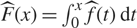 $\hat F(x) = \int_0^x {\kern 1pt} \hat f(t){\kern 1pt} {\rm{d}}t$ represents the respective estimator of the distribution function.
Example 3. Our task is here to verify whether the modified lognormal lifetime distribution is the parent distribution of a random sample X 1,..., XN. Without loss of generality, we may assume that this follows the modified standard lognormal distribution MLN(0, 1,λ,λ,γ) with distribution function given by
 $${F_{\gamma ,\lambda ,\delta }}(x) = \Phi (\ln ((\lambda x{)^\gamma }\exp (\delta x))) = \Phi (\delta x + \gamma \ln x + \gamma \ln \lambda ),\quad \quad x > 0,$$
for some unknown positive λ , λ, and γ, where denotes the standard normal distribution function. Indeed, every modified lognormal distribution function
 $${F_{\gamma ',\lambda ',\delta ',\mu ,\sigma }}(x) = \Phi ({{\delta '} \over \sigma }{\kern 1pt} x + {{\gamma '} \over \sigma }\ln x + {{\gamma '\ln \lambda ' - \mu } \over \sigma })$$
for any μ ∊ ℝ and σ > 0 may be represented as (49) with  $\delta = {{\delta '} \over \sigma }$,
 $\gamma = {{\gamma '} \over \sigma }$, and λ = λ ′ exp
 $( - {\mu \over \sigma })$. Example 2(6) shows that the standard lognormal G-generalized ageing intensity function with G(x) = Φ (ln x) of the distribution function (49) is equal to
 ${L_{G,{F_{\gamma ,\lambda ,\delta }}}}(x) = \gamma + \delta x$, x > 0. We check whether the respective ageing intensity estimator (48) is an accurate approximation of a linear function.
To illustrate the idea we perform the following simulation study. We generate N independent random variables X 1,..., XN with an MLN(0, 1,λ,λ,γ) distribution by means of the two- step procedure. First, using the function lognrnd of MATLAB® with μ = 0 and σ = 1 we generate standard lognormal random variables Y 1,..., YN. Then we obtain modified log- normal MLN(0, 1,λ,λ,γ) random variables by solving numerically (with use of MATLAB) the Lambert equations (λ Xi)λ exp (γ Xi) = Yi with respect to Xi. In order to calculate G-generalized ageing intensity function estimate, we adapt a kernel density estimator (see [Reference Bowman and Azzalini5]) using the ksdensity function available in MATLAB,
 $$\hat f(x) = {1 \over {N{\kern 1pt} h}}\sum\limits_{j = 1}^N K({{x - {X_j}} \over h}),$$
where K is a chosen kernel smoothing function and h is a bandwidth. Then the kernel estimator of the distribution function is equal to
 $$\hat F(x) = {1 \over N}\sum\limits_{j = 1}^N I({{x - {X_j}} \over h}),$$
where  $I(x) = \int_{ - \infty }^x K(t){\kern 1pt} {\rm{d}}t$. The resulting G-generalized ageing intensity function estimate has the form
 $${\hat L_{G,\hat F}}(x) = {{x{\kern 1pt} {1 \over {N{\kern 1pt} h}}\sum\limits_{j = 1}^N K({{x - {X_j}} \over h})} \over {{G^{ - 1}}({1 \over N}\sum\limits_{j = 1}^N I({{x - {X_j}} \over h})){\kern 1pt} g({G^{ - 1}}({1 \over N}\sum\limits_{j = 1}^N I({{x - {X_j}} \over h})))}},$$
where G −1(x) = exp (Φ−1(x)) and 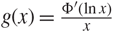 $g(x) = {{\Phi '(\ln x)} \over x}$ are the quantile function and the density function of the standard lognormal distribution LN(0, 1) respectively (calculated in MATLAB using the functions logninv and lognpdf).
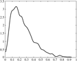
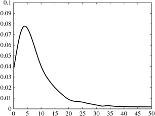
Density estimator  $\hat f$ for the data from Example 3.

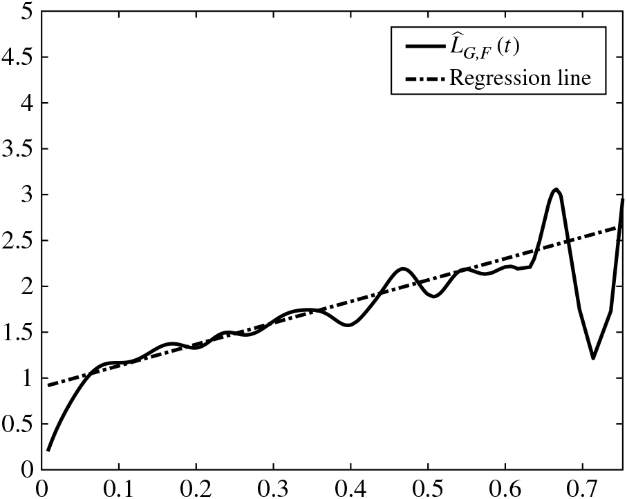
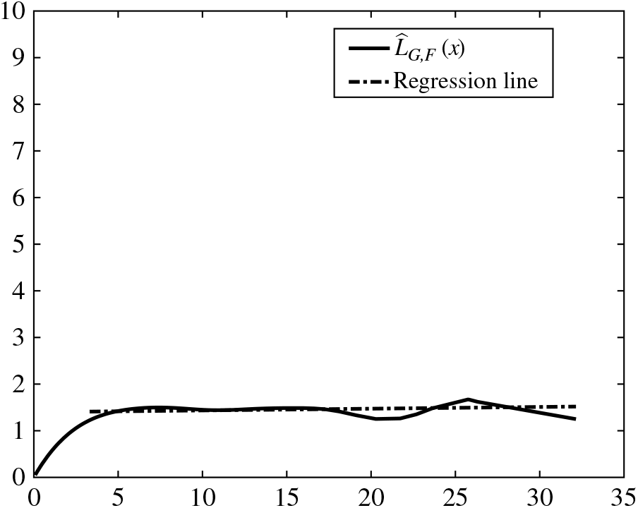
Lognormal ageing intensity estimator  ${\hat L_{G,F}}$ and adjusted regression line for the data from Example 3.

In our experiment we generate N = 1000 independent modified lognormal random variables with parameters λ = 1, λ = 3, and γ = 2. For estimation purposes we choose the normal kernel function and the bandwidth h = 0.02. The plot of the density estimator is presented in Figure 1.
A visual analysis of the graph does not enable us to decide whether the density function belongs to the modified lognormal family. However, looking at the graph of the respective standard lognormal generalized ageing intensity  ${\hat L_{G,\hat F}}$ we immediately notice that it does not depart much from a linear function, especially after removing a few outlying values at the right-hand end (see Figure 2). This gives a reasonable premise for accepting our hypothesis.
A more formal justification is provided by the following statistical procedure. First, we calculate the least squares estimates of the slope and the intercept. For our data they amount to  $\hat \delta = 2.3369$ and
 $\hat \gamma = 0.9002$, respectively.
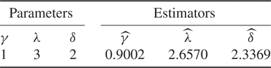
Parameters of MLN(0, 1,γ,λ,δ).

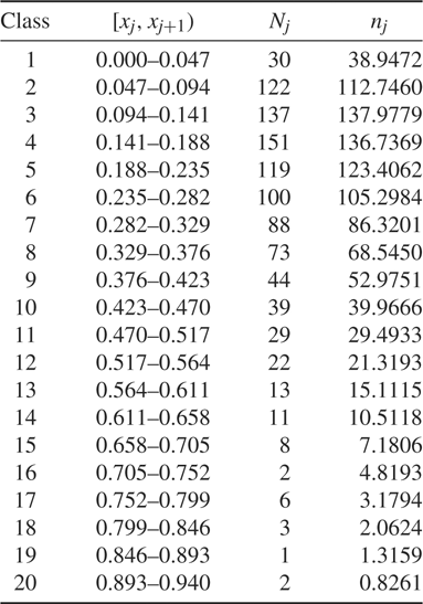
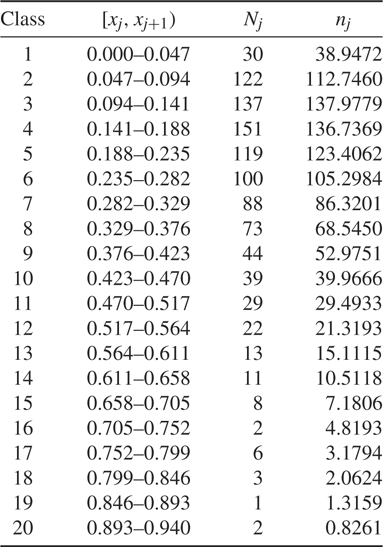
Grouped data and respective values of empirical and theoretical frequency.
Then we determine
 $$\hat \lambda = \exp ( - {1 \over {N{\kern 1pt} \gamma }}\sum\limits_{i = 1}^N (\gamma {\kern 1pt} \ln {X_i} + \delta {\kern 1pt} {X_i})),$$
which maximizes the likelihood function with the parameters γ and λ replaced by their linear regression estimates. Here we obtain  $\hat \lambda = 2.6570$. The theoretical parameters of MLN(0, 1,λ,λ,γ) and their estimators are compared in Table 1. We note that the estimators based on the empirical generalized ageing intensity are quite accurate.
Finally, to check whether our data actually fit the modified lognormal lifetime distribution we use the chi-square goodness-of-fit test for compound parametric hypotheses.
Using the function histogram we group the data into k = 20 classes of observations falling into intervals [xj, x j+1) = [xj, xj + δ x), j = 1,..., k, of length x = 0.047. The empirical frequency of the jth class is denoted by Nj = Nj(X 1,..., XN). The theoretical frequencies are based on the modified lognormal distribution with the parameters replaced by the estimators, and are equal to  ${n_j} = N[{F_{\hat \gamma ,\hat \lambda ,\hat \delta }}({x_{j + 1}}) - {F_{\hat \gamma ,\hat \lambda ,\hat \delta }}({x_j})]$. The classes, together with their empirical and theoretical frequencies, are presented in Table 2.
Kernel density estimator  $\hat f$ for the data from Example 4.

The function chi2gof of MATLAB automatically glues together the last five classes with low frequencies, calculates the value of the chi-square statistics χ 2 = 7.3056 with ν = 12 degrees of freedom, and determines the respective p-value, p = 0.8368. It follows that the hypothesis that the considered data follow the modified lognormal distribution should not be rejected at all the significance levels α < 0.8368.
Example 4. Now we consider a real dataset corresponding to remission times (in months) of a random sample of 128 bladder cancer patients presented in [15]. The data are: 0.08, 2.09, 3.48, 4.87, 6.94, 8.66, 13.11, 23.63, 0.20, 2.23, 3.52, 4.98, 6.97, 9.02, 13.29, 0.40, 2.26, 3.57, 5.06, 7.09, 9.22, 13.80, 25.74, 0.50, 2.46, 3.64, 5.09, 7.26, 9.47, 14.24, 25.82, 0.51, 2.54, 3.70, 5.17, 7.28, 9.74, 14.76, 26.31, 0.81, 2.62, 3.82, 5.32, 7.32, 10.06, 14.77, 32.15, 2.64, 3.88, 5.32, 7.39, 10.34, 14.83, 34.26, 0.90, 2.69, 4.18, 5.34, 7.59, 10.66, 15.96, 36.66, 1.05, 2.69, 4.23, 5.41, 7.62, 10.75, 16.62, 43.01, 1.19, 2.75, 4.26, 5.41, 7.63, 17.12, 46.12, 1.26, 2.83, 4.33, 5.49, 7.66, 11.25, 17.14, 79.05, 1.35, 2.87, 5.62, 7.87, 11.64, 17.36, 1.40, 3.02, 4.34, 5.71, 7.93, 11.79, 18.10, 1.46, 4.40, 5.85, 8.26, 11.98, 19.13, 1.76, 3.25, 4.50, 6.25, 8.37, 12.02, 2.02, 3.31, 4.51, 6.54, 8.53, 12.03, 20.28, 2.02, 3.36, 6.76, 12.07, 21.73, 2.07, 3.36, 6.93, 8.65, 12.63, 22.69.
For the given data, the plot of the normal kernel density estimator (see [Reference Bowman and Azzalini5]) obtained by the ksdensity function available in MATLAB is presented in Figure 3.
Reference [Reference Rady, Hassanein and Elhaddad22] defined the power Lomax distribution function POLO(α, β, λ)as
 $${F_{\alpha ,\beta ,\lambda }}(x) = 1 - {1 \over {{{({1 \over \lambda }{x^\beta } + 1)}^\alpha }}},\quad \quad x \in (0, + \infty ),\;\alpha ,\beta ,\lambda > 0,$$
and claimed that it provides the best fit to the data with estimates of parameters  $\tilde \alpha = 2.0701$,
 $\tilde \beta = 1.4276$, and
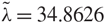 $\tilde \lambda = 34.8626$ determined by the maximum likelihood method. They were calculated by solving numerically three complicated equations with respect to the parameters.
Based on the findings of [Reference Rady, Hassanein and Elhaddad22], we use the generalized ageing intensity approach to get a simpler and more precise data fitting procedure. First we assume that α = 2. We adopt the presumption that natural phenomena and processes are well described and more easily comprehended using simple models. The other prerequisite is that numerical procedures of calculating multivariate maximum likelihood estimators are often unstable and inaccurate.
Estimator  ${\hat L_{G,\hat F}}$ and adjusted regression line for the data from Example 4.

We admit that β and λ may take on arbitrary positive values, because they represent the location and scale parameters when we express the remission times in the logarithmic scale. Indeed,
 $${F_{\alpha ,\beta ,\lambda }}(\exp (x)) = 1 - {1 \over {{{[\exp (\beta x - \ln \lambda ) + 1]}^\alpha }}},\quad \quad \ln \lambda \in ,\quad \mathbb R \beta > 0.$$
In order to verify that POLO(2,β,λ) fits the bladder cancer data with high accuracy, we use the notion of a G-generalized ageing intensity function with
 $$G(x) = 1 - {(1 + x)^{ - 2}},\quad \quad x \in (0, + \infty ),$$
the standard Lomax distribution function with the frailty parameter 2. It has the density function
 $$g(x) = 2(1 + x{)^{ - 3}}$$
and quantile function
 $${G^{ - 1}}(x) = (1 - x{)^{ - {1 \over 2}}} - 1.$$
If F 2,β,λ is actually the POLO(2,β,λ) distribution function, then
 $${L_{G,{F_{2,\beta ,\lambda }}}}(x) = \beta ,\quad \quad x \in (0, + \infty ).$$
We check whether the G-generalized ageing intensity estimator (48) taking the form
 $${\hat L_{G,\hat F}}(x) = {{x{\kern 1pt} \hat f(x)} \over {2[1 - \hat F(x)](1 - {{[1 - \hat F(x)]}^{{1 \over 2}}})}}$$
for G presented above and the normal kernel estimates of the density and distribution functions  $\hat f$ and
 $\hat F$, respectively, is an accurate approximation of a constant function. The function with the graph presented in Figure 4, especially after ignoring several extreme observations, approximates a constant function well, and strongly justifies the belief that the data are well modeled by the POLO(2, β, λ) random variables.
The following statistical procedure allows us to substantiate the statement more rigorously. First we evaluate the least squares estimate 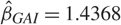 ${\hat \beta _{GAI}} = 1.4368$ of the constant value of
 ${\hat L_{G,\hat F}}$ Plugging it into the log-likelihood function
 $$l(2,\beta ,\lambda ,{x_1} \ldots ,{x_n}) = n\ln 2 + n\ln \beta + 2n\ln \lambda + (\beta - 1)\sum\limits_{i = 1}^n \ln {x_i} - 3\sum\limits_{i = 1}^n \ln (\lambda + x_i^\beta )$$
and maximizing it with respect to λ, which consists in determining the solution to the equation
 $$\sum\limits_{i = 1}^n {1 \over {{1 \over \lambda }x_i^{{{\hat \beta }_{GAI}}} + 1}} = {{2n} \over 3},$$
we obtain  ${\hat \lambda _{GAI}} = 33.9551$
Reference [22] used the Kolmogorov test (and some of its modifications) for checking whether the bladder cancer data match the 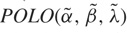 $POLO(\tilde \alpha ,\tilde \beta ,\tilde \lambda )$ distribution with the parameters estimated by the maximum likelihood method. They obtained the test statistic Dn = 0.0351, and a resulting high p-value of p = 0.9960. Repeating their approach on our hypothesis
 $POLO(2,{\hat \beta _{GAI}},{\hat \lambda _{GAI}})$, we obtain a smaller value of the Kolmogorov test statistic Dn = 0.0347, and consequently an even higher p-value of p = 0.9966.
Moreover, we compare [Reference Rady, Hassanein and Elhaddad22] and our hypotheses using the chi-square test, which has a much better theoretical background for verifying the goodness of fit of compound hypotheses. First, using the function histogram we group the data into k = 30 classes of observations falling into equally sized partition subintervals of the interval containing the data. Since the data are mostly concentrated close to 0, some intervals with large observations contain few values; they are glued together by the program, resulting in a reduction of the number of classes to k = 7. Under the POLO(α, β, λ) hypothesis, the distribution of the chi-square test statistic based on the maximum likelihood estimators proposed by [Reference Rady, Hassanein and Elhaddad22] is asymptotically approximated by a chi- square distribution with three degrees of freedom. The value of the test statistic is 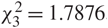 $\chi _3^2 = 1.7876$, which gives a p-value for the test of p = 0.6176. Verifying our hypothesis with the parameter estimates based on the generalized ageing intensity function, we determine the value
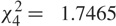 $\chi _4^2 = 1.7465$ for the chi-square statistic with four degrees of freedom, which implies a substantially greater p-value amounting to p = 0.7822. This shows that our hypothesis essentially better fits the bladder cancer remission time data of [Reference Lee and Wang15] than that proposed in [Reference Rady, Hassanein and Elhaddad22].
Acknowledgements
The author is grateful to two anonymous referees and the associate editor for a number of valuable comments which enabled her to correct mistakes and improve the presentation of the results.