1. INTRODUCTION
Due to the limited energy supply and narrow range of observations of a single Autonomous Underwater Vehicle (AUV), many practical underwater exploration missions have gone beyond the ability of a single AUV. The multi-AUV system is a new research area, concentrating on the aspects of applicability, robustness and scalability. For the multi-AUV system (Luo et al., Reference Luo, Chakraborty and Sycara2014; Javier et al., Reference Javier, Dario and Yadira2015; Cao and Zhu, Reference Cao and Zhu2015; Sahar et al., Reference Sahar, Anis, Omar, Habib, Hachemi, Mohamed-Foued and Yasir2014; Jaillet and Porta, Reference Jaillet and Porta2013), it is important to improve the efficiency of the underwater work with reasonable task assignment and path planning under the prevailing conditions. Task assignment and path planning is a technique to control a set of AUVs to access a target point with an optimal path based on algorithms (Huang et al., Reference Huang, Zhu and Sun2016). There has been some research on task assignment and path planning of multi-AUV systems. Kulkarni and Pompili (Reference Kulkarni and Pompili2013) developed a task allocation framework for networked AUVs that work as a team to accomplish critical missions. Ren and Mei (Reference Ren and Mei2013) applied an ant colony algorithm to solve the task allocation problem so that an underwater glider deals with multiple tasks according to the tasks’ situations. The above algorithms can be used to assign different tasks, but they do not have the ability to self-regulate. The efficiency is low because of limited collaboration between AUVs.
In recent years, self-organising neural networks have been widely used in the task assignment and path planning of multi-AUV systems because of their competitive characteristics and self-learning abilities. A self-organising neural network was first proposed by Kohonen (Reference Kohonen1998) and it was mainly used for dynamic regional classification of the input vector. When it is applied to task assignment of multiple robots, the targets will be included, divided and assigned automatically to the most suitable robot. Zhu and Yang (Reference Zhu and Yang2006; Reference Zhu and Yang2012) applied a self-organising neural network to the task assignment and path planning of a multi-robot system. The algorithm they proposed can make each robot reach the target along the shortest path under the premise that the multi-robot system covers all the targets with minimal total energy consumption and can effectively solve the situation that the number of robots and the number of targets are unknown. Aluizio and Santana (Reference Aluizio and Santana2015) proposed a Self-Organising Map-State Trajectory Generator (SOM-STG) to plan and control legged robot locomotion. The SOM-STG can construct one or more gaits for a simulated robot with six legs and control the robot with any of the gaits learned, and can smoothly swap gaits. In addition, the SOM-STG can learn to construct a state trajectory from observing an animal in locomotion. All of the methods above are for ground mobile robots, and the research of task assignment and path planning for a multi-AUV system is rare.
Inspired by the applications of the SOM algorithm in multi-agent systems, Huang et al. (Reference Huang, Zhu and Yuan2012), Zhu et al. (Reference Zhu, Huang and Yang2013) and Huang et al. (Reference Huang, Zhu and Ding2014) proposed an integrated multi-AUV dynamic task assignment and path planning algorithm by combining the Self-Organising Map (SOM) neural network and a novel velocity synthesis approach. Task assignment and path planning of a multi-AUV system for static and dynamic objects is discussed within a Three-Dimensional (3D) time-varying ocean environment. This algorithm achieves path planning and navigation through the optimisation and equalisation of each AUV's workload and weight updates by SOM. Although the algorithm in the literature (Huang et al., Reference Huang, Zhu and Yuan2012; Zhu et al., Reference Zhu, Huang and Yang2013; Huang et al., Reference Huang, Zhu and Ding2014) can solve task assignment and path planning of a multi-AUV system, it does not consider obstacles in real environments. Additionally, each AUV speed is based on the weight function of the SOM and is unlimited, allowing the AUVs’ control constraints to be exceeded. This is often referred to as the speed jump problem. When the target is far from the AUV, the SOM solution proposes that the AUV travels a few kilometres or even several tens of kilometres in each navigation step, which also exceeds the AUV's speed or range capability.
Aiming at the problem of speed jump and the absence of an obstacle avoidance capability in the SOM algorithm, a Glasius Bio-inspired Self-Organising Map (GBSOM) (Glasius et al., Reference Glasius, Komoda and Gielen1995) algorithm combined with a Glasius Bio-inspired Neural Network (GBNN) (Luo et al., Reference Luo, Gao, Li, Mo and Jiang2014a; Reference Luo, Gao, Murphey and Jan2014b) and SOM is proposed in this paper. The implementation steps are: (1) 3D GBNN model is established to represent the grid of the 3D underwater working environment. The magnitude of the neural activity at each node of the GBNN is calculated. (2) SOM is used to assign the targets to a set of AUVs and determine the order of the AUVs accessing the target point. (3) The AUVs’ next navigation point can be planned autonomously according to the distribution of the neuron activity in the GBNN. (4) GBNN is updated. By repeating steps (2), (3) and (4), access to all target points can be completed. The GBSOM algorithm is not only able to prioritise the task assignment, but can also effectively plan a collision-free shortest path for the AUV.
The organisation of the paper is as follows. Section 2 defines the multi-AUV system problem to be solved. The traditional SOM algorithm is introduced in Section 3 and an improved GBSOM algorithm based on SOM is then introduced in Section 4. Section 5 provides simulation results and evaluation of the proposed GBSOM algorithm and Section 6 gives the concluding remarks.
2. THE MULTI-AUV SYSTEM PROBLEM
The core issue of a multi-AUV system is to minimise its energy cost. There are two main aspects of the energy loss in the multi-AUV system: task allocation, and AUV path planning. Figure 1 is a schematic diagram of a 3D underwater environment with obstacles, AUVs and targets. In this paper, we assume that the locations of obstacles, targets and AUV are known.
3-D underwater workspace.

To minimise the energy cost of the multi-AUV system, a reasonable task allocation is first given. For each AUV the need to reach the target and the order of arrival is determined and then the optimal path is planned. The path of each AUV must be collision-free, and the distance and speed of each AUV must meet the kinematics requirements.
The subject of this paper is the task allocation and path planning of a multi-AUV system. The task allocation problem includes one-to-one and one-to-many. The path planning problem includes obstacle avoidance and speed hopping. In this paper, the initial positions of AUVs and targets are required to meet the following principles: The initial location of the AUVs and targets needs to contain all the situations mentioned in this article (one-to-one and one-to-many task assignment and obstacle avoidance). Therefore, in the design of the simulation environment, the initial position of the AUV and the target is not randomly assigned: the locations of AUVs and the targets are chosen to model different task assignment and obstacle avoidance problems. For example, for the task assignment in Figure 1, R2 and R3 might have two corresponding targets and R1, R4 and R6 might be considered to have only one corresponding target. All task assignments are presented in the simulation environment. For path planning, there is no linear path between each target and its corresponding AUV in the designed simulation environment to meet the collision-free requirement. In this way the design of the initial environment can test the performance of the proposed GBSOM algorithm in this paper.
3. TRADITIONAL SOM TASK ASSIGNMENT ALGORITHM
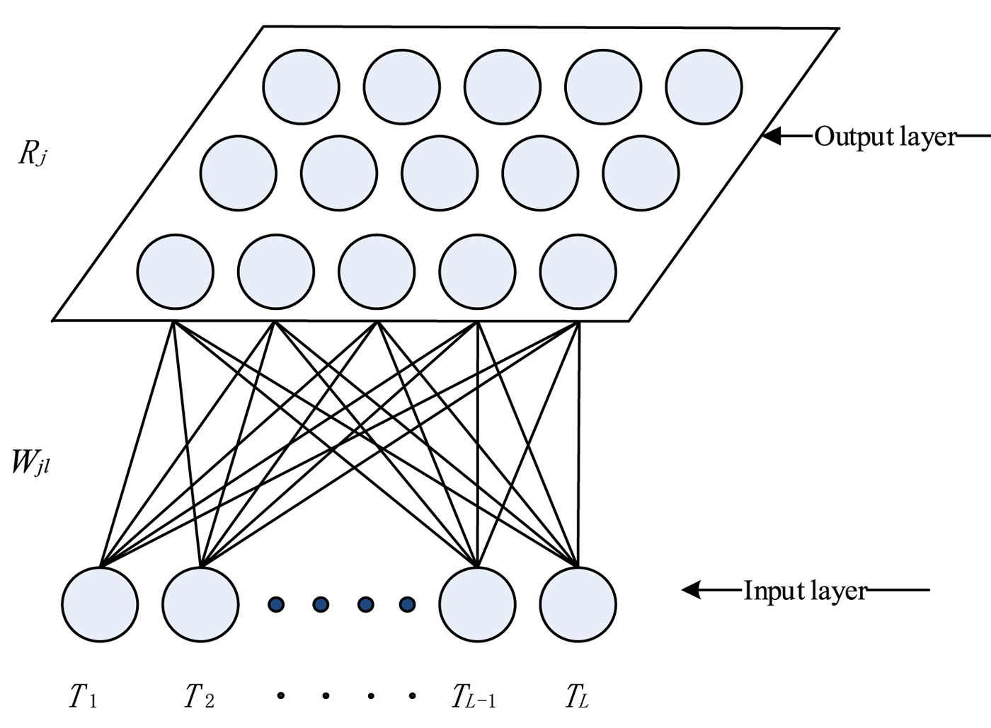
A SOM algorithm is an unsupervised clustering algorithm, which does not need to be trained in advance. It can automatically cluster data according to a certain type of attribute. The distance between an AUV and the target can be used as a clustering attribute in multi-AUV task assignment. The traditional SOM algorithm is composed of two layers of neurons, which are the input and output layers. In the input layer, the external information is collected at each neuron of the output layer through a weight vector. The competitive layer (i.e. the output layer) is responsible for the comparison and analysis of input patterns, finding the rules and classifying them.
In multi-AUV task assignment, the coordinates of the target are selected as the input layer, and the coordinates of the current AUV is selected as the output layer. The network structure of SOM is shown in Figure 2. The SOM algorithm can be divided into the following parts: (1) the selection of the winning neuron; (2) the determination of the neighbourhood function; (3) the update of the weight.
The network structures of SOM.

3.1. The selection of the winning neuron
The principle of the winning neuron selection is the most similar to the clustering attribute. The Euclidean distance of the attribute is usually used to represent the degree of approximation of the attribute; the smaller the Euclidean distance the more similar the attribute. The winner selection rule is obtained by the following expression:
 $$[P_j]\Leftarrow \min (D_{jl}, j=1,2,3,\ldots,J; l=1,2,3,\ldots,L)$$
where [P j ] denotes that the j-th neuron is the selected winner to the l-th input neuron. D jl represents the Euclidean distance between the j-th output node and the l-th input neuron. The Euclidean distance calculation between two neurons is defined as:
 $$|T_l-R_j| = \sqrt{\lpar x_{l}-w_{jx}\rpar ^2 + \lpar y_{l}-w_{jy}\rpar ^2 + \lpar z_{l}-w_{jz}\rpar ^2}$$
Tl = (xl , yl , zl ) represents the coordinates of the l-th input neural node which represents the target location. Rj = (wjx , wjy , wjz ) are the coordinates of output neurons which represent one specific AUV location.
3.2. The determination of the neighbourhood function
When the winning neuron of the SOM network is selected, the next step is to determine the neighbourhood function. The neighbourhood function determines the degree of attraction of the input neurons to the winning neuron and its neighbourhood. The Gauss function is generally selected as the neighbourhood function, which is described as follows:
 $$f(d_m, G) = \left\{ \matrix{ e^{-d_m^2/G^2(t)}, & d_m \leq \lambda \cr 0, \hfill& d_m \gt \lambda \hfill} \right.$$
 $$G(t) = (1-\beta)^t G_0$$
where
 $d_{m} = |N_{m} - N_{j}|$
represents the distance between the m-th output neuron and the winning neuron j. λ is the neighbourhood radius and β is the decay rate. The convergence time of the SOM neural network is determined by the value of β and is proportional to its magnitude. The AUV navigation step size in the neighbourhood can be controlled by setting the value of β and G
0, which can control the accuracy of AUV navigation.
The neighbourhood function is determined according to the actual situation. When one task requires only one AUV, λ should be selected to be 0 to use the AUV efficiently. When one task requires multiple AUVs at the same time, the value of λ should be selected as a suitable constant.
3.3. The update of the weight
In this paper, the weight of the SOM equals the position of the AUV. When the neighbourhood function is determined, the last step of the SOM algorithm is to update the weights. The purpose of the weight updating is to make the SOM algorithm converge, which is to make the AUV close the target point in the multi-AUV system task assignment.
 $$R_j(t+1) = \left\{\matrix{ R_j(t) + \alpha \times f(d_m, G) \times (T_l-R_j(t)), & D_{jl} \gt D_{\min} \cr T_l, \hfill& D_{jl} \leq D_{\min} \hfill} \right.$$
Rj = (wjx , wjy , wjz ) represents the position coordinates of the j-th AUV. Tl = (xl , yl , zl ) represents the position coordinates of the l-th target. α is the learning rate and the range of α is 0 < α ≤ 1. D min represents the minimum distance from the AUV to the target. When the distance between the AUV and the target is less than or equal to D min, the AUV has arrived at the target. D jl is a relevant Euclidean distance value between the winning AUV and the corresponding target position.
From the above description, the traditional SOM algorithm has been found to have the following shortcomings. First, the path planned by the SOM algorithm is a straight line, so the SOM algorithm cannot avoid obstacles effectively. Second, since the weight update function of the SOM corresponds to the navigational distance between the AUV and the target from using Equation (5), in practical applications there is a problem of speed jumps: the initial update may be so large as to generate a speed requirement beyond that of the AUV. In reality, during the early iterations of the SOM algorithm, the AUV might be asked to sail many kilometres in a very short period of time; far exceeding the AUV's speed and range capability.
4. THE GLASIUS BIO-INSPIRED SELF-ORGANISING MAP (GBSOM)
In order to avoid these two problems of traditional SOM algorithms, a 3D GBNN model is established to represent the grid of the 3D underwater working environment. The corresponding dynamic neural network is built on the grid map. Each point in the grid map corresponds to the neural activity of the neurons in the GBNN. The GBNN model is applied to regulate the weights of SOM. The process can be described as follows: select the maximum neural activity point in the AUV's neighbourhood as Pn, and then put Pn into Equation (12) to update the weight of SOM. An integrated GBSOM method is proposed in this section. This section can be divided into two parts. The GBNN algorithm is introduced in Section 4.1, and the combination of GBNN and SOM is introduced in Section 4.2.
4.1. GBNN model
The GBNN algorithm in this paper is a kind of discrete Hopfield-type neural network (Hopfield and Tank, Reference Hopfield and Tank1985). Its kinetic model is as follows:
 $$x_i(t+1) = g\left(\sum^{J}_{j=1}\omega_{ij}\times x_j(t)+I_i\right)$$
 $$\omega_{ij} = \left\{\matrix{ e^{-\gamma|i-j|^2}, & |i-j|\leq r \cr 0, \hfill & |i-j| \gt r } \right.$$
 $$g(x) = \left\{\matrix{ 0, \hfill& x \lt 0 \hfill\cr \beta x, \hfill& x\in [0,1] \hfill\cr 1, \hfill& x \gt 1\hfill} \right.$$
In Equation (6), x
i
(t+1) represents the neural activity of the i-th neuron in the neural network at time instance t+1, x
j
(t) is the neural activity of the neuron j which side-connects with the neuron i with time instance t. In Equation (7), ω
ij
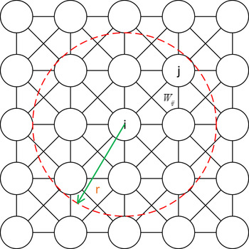
is a symmetric connection coefficient matrix, which is a connection weight coefficient between neuron i and neuron j. |i−j| is the Euclidean distance between neuron i and neuron j. r is a constant value that is more than zero, and the value of r is set as
 $\sqrt{3}$
for the 3D neural network in this paper. The 2D distribution of ω
ij
is shown in Figure 3. In Figure 3, r is a regional radius. Each neuron in the neural network has a right angle or a diagonal connection to the neurons in the region of r. Figure 3 also illustrates the winning point selected from the eight neighbourhoods around the AUV which is seen as a temporary target for the 2D neural network. In the same way, the number of neighbourhoods is 26 for the 3D neural network.
Two-dimensional neural network.

Equation (8) is the transfer function, which limits the output range of the kinetic model, ensuring that the neural activity of the neuron is guaranteed between 0 and 1 and makes the system in a stable state. I i represents the additional input of the i-th neuron. When the neuron is the target, I i is E(E> = 1). When the neuron is an obstacle, I i is −E. Otherwise, I i is 0.
 $$I_i = \left\{\matrix{ E, \hfill& \hbox{if it is a target} \hfill\cr -E, & \hbox{if it is an obstacle} \cr 0, \hfill& \hbox{otherwise}\hfill} \right.$$
For the AUV's current position in the GBNN denoted as P i , P k is the coordinate of the points in k-th P i ’s neighbourhood, and the next moving position P n of AUV can be obtained by
 $$P_n = \arg {\mkern 1mu} \max \{ x_{P_k},P_k \in \mathop U\limits^{\rm o} (P_i,r)\}$$
Since the neural activity of target positions are positive in the GBNN and the neural activity of obstacle positions are negative, the target positions attract the AUV globally while the obstacle areas just push the AUV away to avoid local collisions. For more detail, the reader can refer to Luo et al. (Reference Luo, Gao, Li, Mo and Jiang2014a; Reference Luo, Gao, Murphey and Jan2014b).
4.2. The combination of GBNN and SOM
On the one hand, the distance between the target point and AUV is seen as the competitive attribute in traditional SOM algorithms. The path planned by the SOM algorithm is a straight line, so the traditional SOM algorithm cannot avoid obstacles in practice. On the other hand, the update strategy of the SOM algorithm is successive approximation, and the step length of each update is gradually reduced. In practice, the step size updated is very large at the initial time, which causes the speed jump problem.
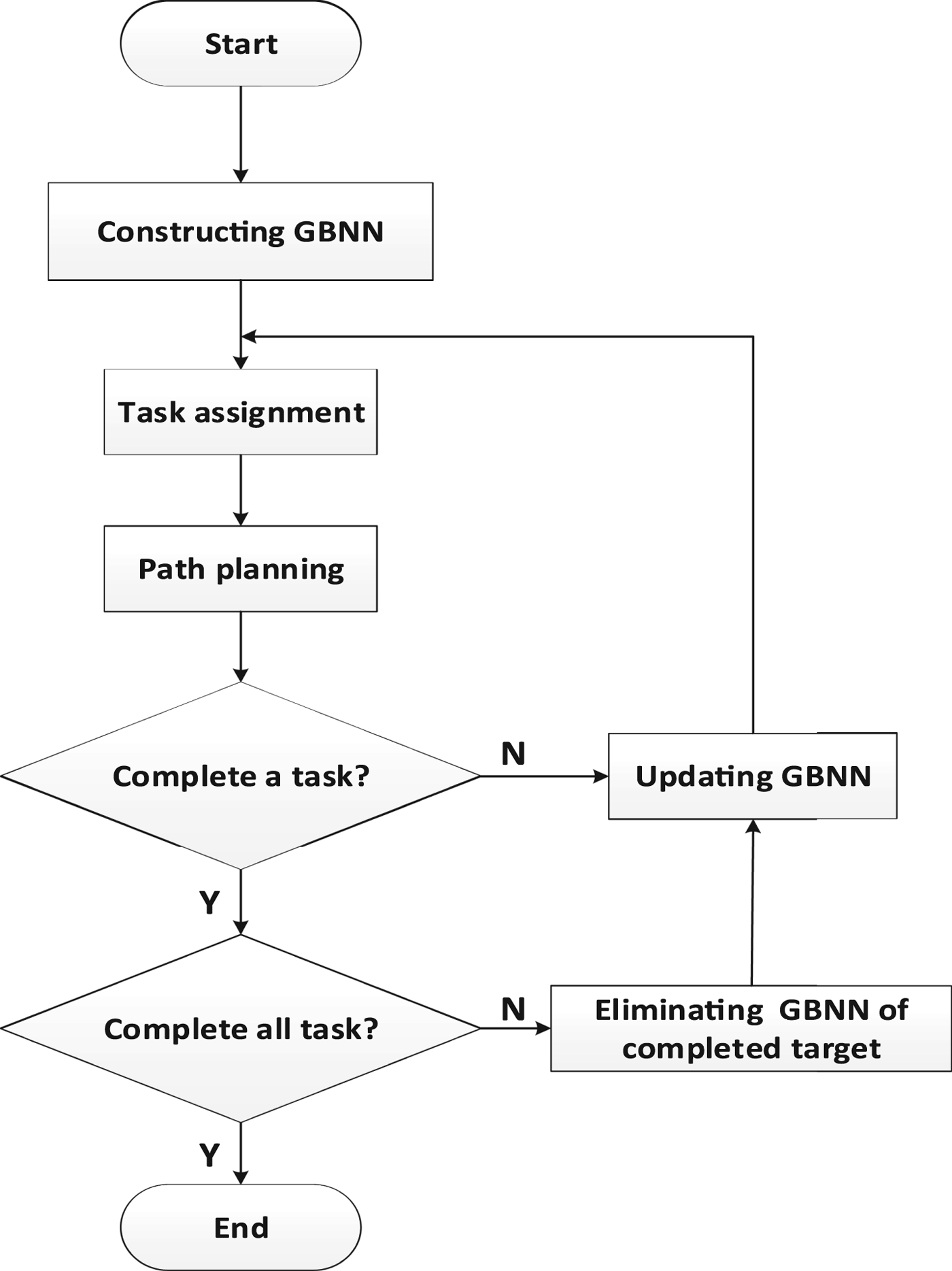
Task assignment and path planning are continuously implemented in the GBSOM algorithm, until the corresponding AUV reaches the corresponding target. The flow chart of the GBSOM algorithm is shown in Figure 4.
Flow chart of the GBSOM algorithm.

The specific steps of the GBSOM algorithm are as follows:
-
(1) A corresponding GBNN is constructed for each target point.
-
(2) Task assignment is implemented.
AUV Task assignment can be divided into two categories. The first is one AUV corresponding to only one target. The second is one AUV corresponding to multiple targets. The first case is relatively simple and only needs to match one AUV with one target. For the second case, due to one AUV corresponding to multiple targets, the order of the corresponding targets should be determined based on the shortest total distance after the magnitude of the neural activity for each AUV/target pair has been assessed and the relevant AUV/target combination chosen; that is, task assignment has been conducted. Equation (11) is used to complete the task assignment.
 $V(P_{T_{l}}, P_{R_{j}})$
represents the neural activity of the j-th AUV in the GBNN of l-th target, where R
j
represents the final winning AUV corresponding to the target T
l
.
 $$(T_l, R_j) \Leftarrow \arg\,\max\,\max(V(P_{T_l}, P_{R_j}))\quad l=1,2,3,\ldots,L;\quad j = 1,2,3,\ldots,J$$
-
(3) Path planning is performed on the basis of the completion of task assignment.
After the AUV's next motion direction location P n is obtained by Equations (6) and (10), to avoid the sharp speed jumps of AUV in SOM path planning, the weight of the SOM is updated:
 $$R_j(t+1) = \left\{\matrix{ R_j(t) + \alpha \times f(d_m, G) \times (P_n-R_j(t)), & D_{jl} \gt D_{\min} \cr P_n, \hfill& D_{jl} \leq D_{\min}} \right.$$
Pn = (xn , yn , zn ) are the coordinates of the AUV in the next moving direction and Rj = (wjx , wjy , wjz ) is the SOM output neuron which represents the AUV position. R j (t) represents the coordinates of the AUV at the present time, R j (t+1) represents the coordinates of the AUV at the next time marker. Compared with the update rule for the winning AUV in Equation (5), as the distance between neighbouring grids is short in the grid map, and AUVs always move toward a neighbouring grid of their current location based on Equation (12), Pn – Rj (t) must be the appropriate value and meet the AUV's speed control constraint (unit speed one). Therefore, AUVs do not experience sharp speed jumps. In addition, due to the GBNN inhibiting the AUV from hitting obstacles, the path planning method based on GBNN can avoid either static or dynamic obstacles. Thus, the proposed GBSOM multi-AUV task assignment and path planning algorithm is valid in an underwater environment with random motion of target location and obstacles.
-
(4) Determine whether the task is completed.
If the task is completed, then the mission is over. Otherwise, the GBNN is updated and the second and third steps are repeated.
5. SIMULATION STUDIES
The simulation of the underwater environment takes place in a 25 metre 3D grid map with the length of each grid cube set to 1 metre. A corresponding neural network structure is built for each target on the grid map and the neural activities of all neurons are initialised to 0. In addition, the shape and size of the AUV are not considered in the simulation, which means it is simplified as a particle. All the chosen parameters of the GBSOM algorithm in the simulation experiments are listed in Table 1.
Control parameters.

In order to test the effectiveness of the algorithm, the simulation results of the task assignment and path planning of a multi-AUV system are shown below.
5.1 The task assignment and path planning in a 3D static environment
5.1.1. One AUV corresponds to one target
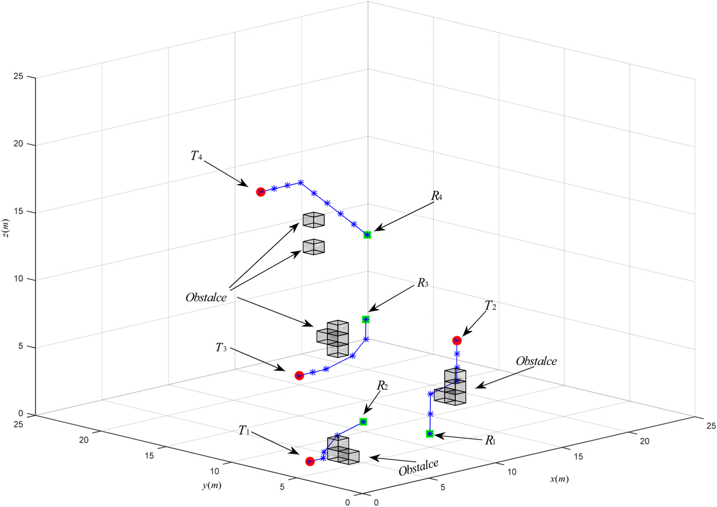
The amount of AUVs is equal to the number of targets, which means one AUV is assigned to one target. The simulation results of the task assignment and path planning of multi-AUV in a 3D static environment are shown in Figure 5. The initial positions of the AUVs are: R 1(10,5,1), R 2(5,5,3), R 3(15,15,6), R 4(20,20,10). The initial positions of targets are: T 1(1,5,1), T 2(13,6,7), T 3(10,15,3), T 4(12,20,15).
The simulation diagram of one AUV corresponding to one target in 3D.

One AUV corresponds to one target, which is the simplest and most basic case. Only one SOM competition is needed to complete the AUV task assignment. The initial task assignment is completed by selecting the AUV with the highest neural activity in the GBNN of each target.
Table 2 shows the neural activity of each AUV in the GBNN of each target at the initial state in task assignment, and the red region is the maximum activity for each T
l
. The initial task assignment is accomplished by selecting the AUV whose neural activity is maximal in the GBNN of each target. The following briefly takes T
1 as an example to analyse the task assignment. From Table 2, the neural activities of four AUVs in the GBNN of T
1 are:
 $V(P_{R_{1}}, P_{T_{1}}) = 2{\cdot}04E\hbox{-}14, V(P_{R_{2}}, P_{T_{1}}) = 5{\cdot}95E\hbox{-}7, V(P_{R_{3}}, P_{T_{1}}) = 4{\cdot}03E\hbox{-}42, V(P_{R_{4}}, P_{T_{1}}) = 1{\cdot}03E\hbox{-}28$
.
The neural activity of each AUV in the GBNN of each target at initial state.

Since the neural activity of
 $V(P_{R_{2}}, P_{T_{1}})$
is maximal, T
1 is assigned to R
2. Similarly, the results of the initial assignment for the remaining target points are T
2-R
1, T
3-R
3, and T
4-R
4. After the completion of task assignment, the specific path of the AUV needs to be planned. The following briefly takes T
1-R
2 as an example to analyse the path planning.
Table 3 shows the GBNN neural activity in the 26 neighbourhoods of R 2, and the red region is the maximum activity in the 26 neighbourhoods of R 2. The P n point whose neural activity is maximal among the 26 neighbourhoods of R 2’s current position is selected as the next point in path planning. Firstly, P n is (4, 6, 2) computed by Equation (10). Secondly, P n is taken into Equation (12), which means the specific path panning of P n-R 2 is completed. Repeat these two steps until R 2 reaches the corresponding T 1.
The GBNN neural activity in the 26 neighbourhoods of R 2.

5.1.2. One AUV corresponds to multiple targets
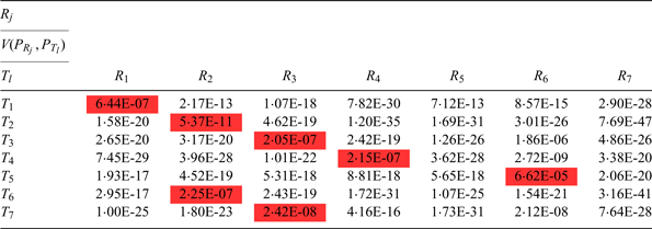
The simulation results of the task assignment and path planning of one AUV corresponding to multiple targets in a 3D static environment are shown in Figure 6. The initial positions of the AUVs are: R 1(16,4,1), R 2(8,4,2), R 3(4,16,3), R 4(7,18,18), R 5(20,5,6), R 6(10,15,10), R 7(20,20,16). The initial positions of targets are: T 1(14,10,3), T 2(1,4,2), T 3(8,16,6), T 4(9,14,16), T 5(12,12,10), T 6(4,4,5), T 7(5,17,8). For the second case in AUV task assignment, one competition can only determine to which targets each AUV corresponds, but cannot determine the order of AUVs in reaching the target points. The order of arrival should be determined in order to complete the task assignment, so it can be determined by adopting the second competition which is shown in Equation (11).
3D simulation diagram of one AUV corresponding to multiple targets.

The following takes R 2 as an example to briefly analyse. First, the AUV whose neural activity is maximal in its GBNN is chosen for each target, the results of the selection are shown in the red region of Table 4. From Table 4, it can be seen that R 2 corresponds to T 2 and T 6, and the neural activity of R 2 in the GBNN of T 2 and T 6 are V(R 2, T 2) = 5·37E-11, V(R 2, T 6) = 2·25E-7. Inputting the above information into Equation (11), it is found that R 2 reaches T 6 first and then reaches T 2. Similarly, the results of the initial assignment for the remaining target points are R 1-T 1, R 2-T 6-T 2, R 3-T 7-T 3, R 4-T 4, R 6-T 5; R 5 and R 7 do not perform a task. After the completion of task assignment, the specific path of the AUV needs to be planned. The following briefly takes T 7-R 3 as an example to analyse the path planning. Table 5 shows the GBNN neural activity in the 26 neighbourhoods of R 3, and the red region is maximum activity in the 26 neighbourhoods of R 3. The point P n whose neural activity is maximal among the 26 neighbourhoods of R 3 of the current position is selected as the next point in path planning. Firstly, P n is (4, 17, 4) computed by Equation (10). Secondly, P n is taken into Equation (12), which means the specific path panning of P n −R 3 is completed. Repeat these two steps until R 3 reaches the corresponding T 7.
The neural activity of each AUV in the GBNN of each target at the initial state.

The GBNN neural activity in the 26 neighbourhoods of R 3

Comparison in terms of AUV speed for R 3 between SOM and GBSOM algorithm is shown in Table 6 and Figure 7 (blue lines show the GBSOM algorithm and the red lines show the SOM algorithm). The comparison shows that R 3 stops after only five iterations of the SOM algorithm alone; R 3 collides with Obstacle 4. In Table 6 and Figure 7, it is clear that the speeds of SOM navigation are far beyond the AUV's control constraint, but the proposed GBSOM algorithm fully meets these. The next motion direction of the AUV is towards the neighbouring coordinate of its current location based on the proposed GBSOM algorithm. The mobile speed of the AUV must meet its control constraint requirements and the AUVs have no sharp speed jumps. However, the traditional SOM task assignment and path planning algorithms do not consider the constraint of AUV speed, thus, AUV speed jumps will occur when the error Tl -Rj between the AUV's current coordinates R j and corresponding target coordinates T l suddenly change. In particular, the distance between the AUV and the target may reach tens of kilometres at the start times. Equation (5) is used to update the AUV position. The AUV is required to provide a very high speed to keep the algorithm real-time. It is practically impossible for an AUV to achieve such a high speed.
Comparison in terms of speed for R3 between SOM and GBSOM algorithms.

Comparison of the first ten terms of speed for R 3 between SOM and GBSOM algorithms.

5.2. Task assignment and path planning in a 3D dynamic environment
Obstacles can be divided into static obstacles and dynamic obstacles in the real ocean environment, and it is more complicated to deal with dynamic obstacles.
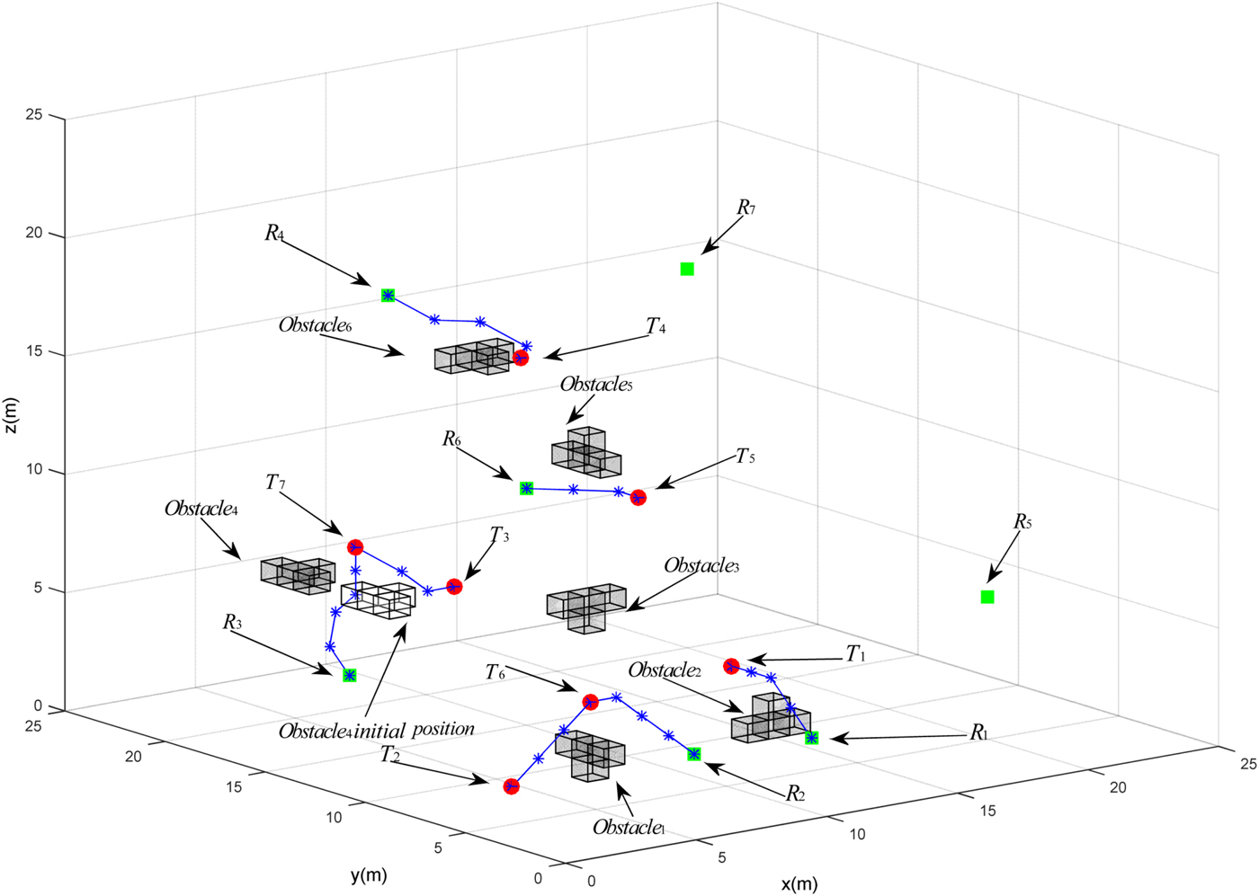
The simulation result of task assignment and path planning in a dynamic environment is shown in Figure 8. Obstacle 4 is a dynamic obstacle. Since Obstacle4 is moving, the moving path of R 3 near Obstacle4 is affected. The dynamic Obstacle4 is far away from the other AUVs, so the impact of the other AUVs’ path planning is not large. Since Obstacle4 is relatively far away from R 3, the path planning of R 3 is basically not affected. With the moving of Obstacle4 and R 3 getting closer to Obstacle4 , the movement of Obstacle4 begins to affect the path planning of R 3. A path to steer clear of obstacles for R 3 is planned when Obstacle4 is not moving. When Obstacle4 is dynamic, Figure 8 shows that R 3 changes the path of the original selection to pass through the initial position of Obstacle4 .
Task assignment and path planning in a dynamic environment.

6. CONCLUSION
A GBSOM algorithm is proposed to complete AUV task assignment and path planning in 3D static and dynamic environments in this paper. The algorithm can overcome the problem of speed jumps and offers obstacle avoidance capabilities missing from traditional SOM algorithms. Simulation results show that the GBSOM algorithm proposed in this paper can not only achieve the task assignment in a 3D underwater environment, but can also avoid static or dynamic obstacles and resolve the speed jump problem. In this paper, the task assignment and path planning are considered under ideal conditions with no ocean current. Ocean currents will be added in the next step of research.
ACKNOWLEDGMENT
This project is supported by the National Natural Science Foundation of China (51575336, 61503239), Creative Activity Plan for Science and Technology Commission of Shanghai (16550720200, 15550722400).