2. Coherent measures, representations

Let $\mathcal{M}([0,1]^2)$ and $\mathcal{M}([0,1])$ denote the space of nonnegative Borel measures on $[0,1]^2$ and [0, 1], respectively. For $\mu \in \mathcal{M}([0,1]^2)$ , let $\mu^x, \mu^y \in \mathcal{M}([0,1])$ be defined by $\mu^x(A) = \mu(A\times [0,1])$ and $\mu^y(B)=\mu([0,1]\times B)$ for all Borel subsets $A,B\in\mathcal{B}([0,1])$ . We begin with the following characterisation of $\mathcal{C}$ .

Recall the definition of the class $\mathcal{R}$ formulated in the previous section. Let us study the connection between this class and the family of all coherent distributions.

Proof of Proposition 1.1. First, we show that the decomposition $m=\mu+\nu$ exists for all $m\in \mathcal{C}$ . Indeed, by virtue of Proposition 2.1, we can find a random vector $(X,Y)\sim m$ defined on some probability space $(\Omega, \mathcal{F}, \mathbb{P})$ such that $X=\mathbb{E}(Z\mid X)$ and $Y=\mathbb{E}(Z\mid Y)$ for some random variable $Z\in[0,1]$ . For a set $C\in\mathcal{B}([0,1]^2)$ , we put

(2.1) \begin{equation} \mu(C) = \int_{\{(X,Y)\in C\}}Z\,\mathrm{d}\mathbb{P}, \qquad \nu(C) = \int_{\{(X,Y)\in C\}}(1-Z)\,\mathrm{d}\mathbb{P}. \end{equation}

Then the equality $m=\mu+\nu$ is evident. Furthermore, for a fixed $A\in \mathcal{B}([0,1])$ ,

(2.2) \begin{equation} \int_{\{X\in A\}}X\,\mathrm{d}\mathbb{P} = \int_{\{X\in A\}}Z\,\mathrm{d}\mathbb{P} = \int_{A}1\,\mathrm{d}\mu^x, \end{equation}

where the first equality is due to $X=\mathbb{E}(Z\mid X)$ and the second is a consequence of (2.1). Moreover, we may also write

(2.3) \begin{equation} \int_{\{X\in A\}}X\,\mathrm{d}\mathbb{P} = \int_{A\times[0,1]}x\,\mathrm{d}m = \int_{A}x\,\mathrm{d}\mu^x + \int_{A}x\,\mathrm{d}\nu^x. \end{equation}

Combining (2.2) and (2.3), we get $\int_{A}(1-x)\,\mathrm{d}\mu^x = \int_{A}x\,\mathrm{d}\nu^x$ for all $A\in \mathcal{B}([0,1])$ . The symmetric condition (the second requirement in Definition 1.1) is shown analogously. This completes the first part of the proof.

Now, pick a probability measure m on $[0,1]^2$ such that $m=\mu+\nu$ for some $(\mu, \nu) \in \mathcal{R}$ . We need to show that m is coherent. To this end, consider the probability space $([0,1]^2, \mathcal{B}([0,1]^2),m)$ and the random variables $X,Y\colon[0,1]^2 \rightarrow [0,1]$ defined by $X(x,y)=x$ and $Y(x,y)=y$ , $x,y\in [0,1]$ . Additionally, let Z denote the Radon–Nikodym derivative of $\mu$ with respect to m: we have $0\le Z \le 1$ m-almost surely and $\mu(C) = \int_{C}Z\,\mathrm{d}m$ for all $C\in\mathcal{B}([0,1]^2)$ . Again by Proposition 2.1, it is sufficient to verify that $X=\mathbb{E}(Z\mid X)$ and $Y=\mathbb{E}(Z\mid Y)$ . By symmetry, it is enough to show the first equality. Fix $A\in \mathcal{B}([0,1])$ and note that

(2.4) \begin{equation} \int_{\{X\in A\}}X\,\mathrm{d}m = \int_{A\times[0,1]}x\,\mathrm{d}m = \int_{A}x\,\mathrm{d}\mu^x + \int_{A}x\,\mathrm{d}\nu^x. \end{equation}

Similarly, we also have

(2.5) \begin{equation} \int_{\{X\in A\}}Z\,\mathrm{d}m = \int_{A\times[0,1]}Z\,\mathrm{d}m = \mu(A\times[0,1]) = \int_{A}1\,\mathrm{d}\mu^x. \end{equation}

Finally, note that by $(\mu, \nu) \in \mathcal{R}$ , the right-hand sides of (2.4) and (2.5) are equal. Therefore, we obtain the identity $\int_{\{X\in A\}}X\,\mathrm{d}m = \int_{\{X\in A\}}Z\,\mathrm{d}m$ for arbitrary $A\in \mathcal{B}([0,1])$ . This yields the claim.

We turn our attention to the characterisation of $\mathrm{ext}(\mathcal{C})$ stated in the previous section.

Proof of Theorem 1.4. For the implication ‘ $\Rightarrow$ ’, let m be an extremal coherent measure and suppose, on the contrary, that $(\mu_1, \nu_1)$ and $(\mu_2, \nu_2)$ are two different elements of $\mathcal{R}(m)$ . We will prove that $m-\mu_1+\mu_2$ and $m-\mu_2+\mu_1$ are also coherent distributions. Because

\begin{align*}m = \frac{1}{2}(m-\mu_1+\mu_2) + \frac{1}{2}(m-\mu_2+\mu_1),\end{align*}

we obtain a contradiction with the assumed extremality of m. By symmetry, it is enough to show that $(m-\mu_1+\mu_2) \in \mathcal{C}$ . To this end, by virtue of Proposition 1.1, it suffices to check that $m-\mu_1+\mu_2$ is a probability measure and $(\mu_2, m-\mu_1) \in \mathcal{R}$ . First, note that $\nu_1=m-\mu_1$ is nonnegative, and fix an arbitrary $A\in \mathcal{B}([0,1])$ . As $(\mu_1, \nu_1)$ and $(\mu_2, \nu_2)$ are representations of m, Definition 1.1 gives

(2.6) \begin{align} \int_{A}1\,\mathrm{d}\mu_1^x = \int_{A}x\,(\mathrm{d}\nu_1^x+\mathrm{d}\mu_1^x) = \int_{A}x\,\mathrm{d}m^x, \nonumber \\[5pt] \int_{A}1\,\mathrm{d}\mu_2^x = \int_{A}x\,(\mathrm{d}\nu_2^x+\mathrm{d}\mu_2^x) = \int_{A}x\,\mathrm{d}m^x, \end{align}

so $\mu_1^x(A)=\mu_2^x(A)$ . Similarly, we can deduce that $\mu_1^y=\mu_2^y$ , which means that marginal distributions of $\mu_1$ and $\mu_2$ are equal. This, together with $m-\mu_1\ge 0$ , proves that $m-\mu_1+\mu_2$ is a probability measure. Next, using (2.6) and $\mu_1^x=\mu_2^x$ , we can also write

(2.7) \begin{equation} \int_{A}(1-x)\,\mathrm{d}\mu_2^x = \int_{A}x\,\mathrm{d}m^x - \int_{A}x\,\mathrm{d}\mu_1^x = \int_{A}x\,\mathrm{d}(m-\mu_1)^x. \end{equation}

In the same way, we get

(2.8) \begin{equation} \int_{B}(1-y)\,\mathrm{d}\mu_2^y = \int_{B}y\,\mathrm{d}(m-\mu_1)^y \end{equation}

for all $B\in \mathcal{B}([0,1])$ . By (2.7) and (2.8), we obtain $(\mu_2, m-\mu_1) \in \mathcal{R}$ , and this completes the proof of uniqueness.

To show the minimality, let m be an extremal coherent measure with the representation $(\mu,\nu)$ (which is unique, as we have just proved). Consider any nonzero $(\tilde{\mu},\tilde{\nu})\in\mathcal{R}$ with $\tilde{\mu}\le \mu$ and $\tilde{\nu}\le \nu$ . Then, by the very definition of $\mathcal{R}$ , $(\mu-\tilde{\mu},\nu-\tilde{\nu})\in\mathcal{R}$ . Therefore, by Proposition 1.1, we get $\alpha^{-1}(\tilde{\mu}+\tilde{\nu}),(1-\alpha)^{-1}(m-\tilde{\mu}-\tilde{\nu}) \in \mathcal{C}$ , where $\alpha=(\tilde{\mu}+\tilde{\nu})([0,1]^2) \in (0,1]$ . We have the identity

\begin{equation*} m = \alpha\cdot(\alpha^{-1}(\tilde{\mu}+\tilde{\nu})) + (1-\alpha)\cdot((1-\alpha)^{-1}(m-\tilde{\mu}-\tilde{\nu})), \end{equation*}

which, combined with the extremality of m, yields $m=\alpha^{-1}(\tilde{\mu}+\tilde{\nu})=\alpha^{-1}\tilde{\mu}+\alpha^{-1}\tilde{\nu}$ . But $(\alpha^{-1}\tilde{\mu},\alpha^{-1}\tilde{\nu})$ belongs to $\mathcal{R}$ , since $(\tilde{\mu},\tilde{\nu})$ does, and hence $(\alpha^{-1}\tilde{\mu},\alpha^{-1}\tilde{\nu})$ is a representation of m. By the uniqueness, we deduce that $(\tilde{\mu}, \tilde{\nu}) = \alpha\cdot(\mu,\nu)$ .

For the implication ‘ $\Leftarrow$ ’, let m be a coherent distribution with the unique and minimal representation $(\mu, \nu)$ . To show that m is extremal, consider the decomposition $m=\beta \cdot m_1+(1-\beta)\cdot m_2$ for some $m_1, m_2 \in \mathcal{C}$ and $\beta \in (0,1)$ . Moreover, let $(\mu_1, \nu_1)\in \mathcal{R}(m_1)$ and $(\mu_2, \nu_2) \in \mathcal{R}(m_2)$ . By the convexity of $\mathcal{R}$ , we have

\begin{equation*} (\mu', \nu') \;:\!=\; (\beta\mu_1 + (1-\beta)\mu_2,\,\beta\nu_1 +(1-\beta)\nu_2) \in \mathcal{R}(m) \end{equation*}

and hence, by the uniqueness, we get $(\mu', \nu')=(\mu, \nu)$ . Then, directly from the previous equation, we have $\beta \mu_1\le \mu$ and $\beta \nu_1 \le \nu$ . Combining this with the minimality of $(\mu, \nu)$ , we get $(\beta\mu_1,\beta\nu_1)=\alpha (\mu,\nu)$ for some $\alpha\in [0,1]$ . Since $m=\mu+\nu$ and $m_1=\mu_1+\nu_1$ are probability measures, this gives $\alpha=\beta$ and hence $(\mu_1, \nu_1)=(\mu, \nu)$ . This implies $m=m_1$ and completes the proof.

3. Extreme points with finite support

In this section we study the geometric structure of the supports of measures belonging to $\textrm{ext}_\mathrm{f}(\mathcal{C}) = \{\eta \in \textrm{ext}(\mathcal{C}) \colon |\mathrm{supp}(\eta)|<\infty\}$ . Our key result is presented in Theorem 3.1—we prove that the support of an extremal coherent distribution cannot contain any axial cycles (see Definition 1.4). Let us emphasise that this property was originally conjectured in [Reference Zhu21]. We start with a simple combinatorial observation: it is straightforward to check that certain special ‘alternating’ cycles are forbidden.

An example of such an alternating cycle is shown in Figure 1.

Figure 1.

An example of an alternating cycle. Red points represent probability masses in $\mathrm{supp}(\mu)$ , while blue points indicate probability masses in $\mathrm{supp}(\nu)$ . Arrows outline a possible transformation of the representation $(\mu,\nu)$ .

Before the further combinatorial analysis, we need to introduce some useful auxiliary notation. For $\mu, \nu \in \mathcal{M}([0,1]^2)$ with $|\mathrm{supp}(\mu+\nu)|<\infty$ , we define a quotient function $q_{(\mu, \nu)}\colon \mathrm{supp}(\mu+\nu) \rightarrow [0,1]$ by

\begin{align*}q_{(\mu, \nu)}(x,y)= \frac{\mu(x,y)}{\mu(x,y)+\nu(x,y)}.\end{align*}

In what follows, we omit the subscripts and write q for $q_{(\mu,\nu)}$ whenever the choice for $(\mu,\nu)$ is clear from the context.

Next, we will require an additional distinction between three different types of points.

1. (i) a lower out point if $q(x,y)< \min(x,y)$ ;

2. (ii) an upper out point if $q(x,y)> \max(x,y)$ ;

3. (iii) a cut point if it is not an out point, i.e. $x\leq(x,y)\le y$ or $y\le q(x,y) \le x$ .

Finally, for the sake of completeness, we include a formal definition of an axial path.

To develop some intuition, it is convenient to inspect the following example.

Example 3.1. Let m be a probability measure given by

\begin{align*} m\bigg(\frac{1}{8},\frac{1}{4}\bigg)=\frac{84}{196}, \qquad m\bigg(\frac{1}{2},\frac{1}{4}\bigg)=\frac{14}{196}, \qquad m\bigg(\frac{1}{2},\frac{3}{4}\bigg)=\frac{14}{196}, \qquad m\bigg(\frac{7}{8},\frac{3}{4}\bigg)=\frac{84}{196}. \end{align*}

There are five observations, which we discuss separately.

1. (i) Consider the decomposition $m=\mu+\nu$ , where $(\mu,\nu)$ is determined by the quotient function

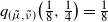
   \begin{align*} q\bigg(\frac{1}{8},\frac{1}{4}\bigg)=\frac{1}{8}, \qquad q\bigg(\frac{1}{2},\frac{1}{4}\bigg)=1, \qquad q\bigg(\frac{1}{2},\frac{3}{4}\bigg)=0, \qquad q\bigg(\frac{7}{8},\frac{3}{4}\bigg)=\frac{7}{8}. \end{align*}
   Using Proposition 3.2, we can check that $(\mu,\nu)\in\mathcal{R}$ . For instance, for $y=\frac{1}{4}$ we get
   (3.3) \begin{equation} \frac{q\big(\frac{1}{8},\frac{1}{4}\big)\cdot m\big(\frac{1}{8},\frac{1}{4}\big) + q\big(\frac{1}{2},\frac{1}{4}\big)\cdot m\big(\frac{1}{2},\frac{1}{4}\big)} {m\big(\frac{1}{8}, \frac{1}{4}\big)+m\big(\frac{1}{2}, \frac{1}{4}\big)} = \frac{\frac{1}{8}\cdot \frac{84}{196}+1\cdot \frac{14}{196}}{\frac{84}{196}+\frac{14}{196}} = \frac{1}{4}, \end{equation}
   which agrees with (3.2). As a direct consequence, by Proposition 1.1, we have $m\in \mathcal{C}$ .

2. (ii) Observe that $\big(\frac{1}{8}, \frac{1}{4}\big)$ and $\big(\frac{7}{8}, \frac{3}{4}\big)$ are cut points, $\big(\frac{1}{2}, \frac{1}{4}\big)$ is an upper out point, and $\big(\frac{1}{2}, \frac{3}{4}\big)$ is a lower out point. Moreover, $\mathrm{supp}(m)$ is an axial path without cycles—see Figure 2.

   Figure 2.

   Support of a coherent distribution m. Purple points (endpoints of the path) are cut points. The red point represents a mass in $\mathrm{supp}(\mu)$ and is an upper out point. The blue point indicates a mass in $\mathrm{supp}(\nu)$ and it is a lower out point.

   

1. (iii) Notably, $(\mu, \nu)$ is a unique representation of m. Indeed, $\big(\frac{1}{8},\frac{1}{4}\big)$ is the only point in $\mathrm{supp}(m)$ with x-coordinate equal to $\frac{1}{8}$ and hence $q\big(\frac{1}{8}, \frac{1}{4}\big)=\frac{1}{8}$ . Accordingly, $q\big(\frac{1}{2}, \frac{1}{4}\big)=1$ is now a consequence of (3.3). The derivation of $q\big(\frac{1}{2}, \frac{3}{4}\big)=0$ and $q\big(\frac{7}{8}, \frac{3}{4}\big)=\frac{7}{8}$ follows from an analogous computation.

2. (iv) Finally, the representation $(\mu, \nu)$ is minimal; let $(\tilde{\mu},\tilde{\nu})\in\mathcal{R}$ satisfy $\tilde{\mu}\le\mu$ and $\tilde{\nu}\le\nu$ . Suppose that $\big(\frac{1}{8}, \frac{1}{4}\big)\in \mathrm{supp}(\tilde{\mu}+\tilde{\nu})$ . Again, as $\big(\frac{1}{8}, \frac{1}{4}\big)$ is the only point in $\mathrm{supp}(m)$ with x-coordinate equal to $\frac{1}{8}$ , we get $q_{(\tilde{\mu},\tilde{\nu})}\big(\frac{1}{8},\frac{1}{4}\big)=\frac{1}{8}$ . Next, assume that $\big(\frac{1}{2}, \frac{1}{4}\big)\in \mathrm{supp}(\tilde{\mu}+\tilde{\nu})$ . 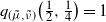As $\tilde{\nu}\big(\frac{1}{2}, \frac{1}{4}\big) \le \nu\big(\frac{1}{2}, \frac{1}{4}\big)=0$ , we have $q_{(\tilde{\mu},\tilde{\nu})}\big(\frac{1}{2}, \frac{1}{4}\big)=1$ . Likewise, we can check that $q_{(\tilde{\mu},\tilde{\nu})}(x,y) = q_{(\mu, \nu)}(x,y)$ for all $(x,y)\in \mathrm{supp}(\tilde{\mu}+\tilde{\nu})$ . From this and Proposition 3.2, we easily obtain that $\tilde{\mu} +\tilde{\nu}=0$ or $\mathrm{supp}(\tilde{\mu}+\tilde{\nu})=\mathrm{supp}(m)$ . For example,

   • if $\big(\frac{1}{2}, \frac{1}{4}\big)\in \mathrm{supp}(\tilde{\mu}+\tilde{\nu})$ , then (3.1) gives $\big(\frac{1}{2}, \frac{3}{4}\big) \in \mathrm{supp}(\tilde{\mu}+\tilde{\nu})$ ;

   • if $\big(\frac{1}{2}, \frac{3}{4}\big)\in \mathrm{supp}(\tilde{\mu}+\tilde{\nu})$ , then (3.2) yields $\big(\frac{7}{8}, \frac{3}{4}\big) \in \mathrm{supp}(\tilde{\mu}+\tilde{\nu})$ .

   Therefore, if $\tilde{\mu}+\tilde{\nu}\not=0$ , then the measure $\tilde{\mu}+\tilde{\nu}$ is supported on the same set as m and $q_{(\tilde{\mu},\tilde{\nu})} \equiv q_{(\mu, \nu)}$ . For the same reason, i.e. using Proposition 3.2 and the path structure of $\mathrm{supp}(m)$ , it follows that $\tilde{\mu}+ \tilde{\nu} = \alpha \cdot m$ for some $\alpha \in [0,1]$ . For instance, by (3.2) for $y=\frac{1}{4}$ , we get

   \begin{align*} \frac{\frac{1}{8}\cdot\tilde{m}\big(\frac{1}{8},\frac{1}{4}\big) + 1\cdot\tilde{m}\big(\frac{1}{2}, \frac{1}{4}\big)} {\tilde{m}\big(\frac{1}{8},\frac{1}{4}\big) + \tilde{m}\big(\frac{1}{2},\frac{1}{4}\big)} = \frac{1}{4}, \end{align*}
   where $\tilde{m}= \tilde{\mu}+\tilde{\nu}.$ Hence $\tilde{m}\big(\frac{1}{8}, \frac{1}{4}\big)\tilde{m}\big(\frac{1}{2},\frac{1}{4}\big)^{-1} = m\big(\frac{1}{8}, \frac{1}{4}\big)m\big(\frac{1}{2}, \frac{1}{4}\big)^{-1}=\frac{84}{14}$ .

1. (v) By the above analysis and Theorem 1.4, we conclude that $m\in\mathrm{ext}_\mathrm{f}(\mathcal{C})$ .

To clarify the main reasoning, we first record an obvious geometric lemma.

We are now ready to demonstrate the central result of this section.

Let us briefly explain the main idea of the proof. For $\eta \in \mathrm{ext}_\mathrm{f}(\mathcal{C})$ , we inductively construct a special axial path contained in $\mathrm{supp}(\eta)$ , which does not contain any cut points (apart from the endpoints). We show that the axial path obtained in this process is acyclic and involves all the points from $\mathrm{supp}(\eta)$ .

Proof of Theorem 3.1. Fix $\eta \in \mathrm{ext}_\mathrm{f}(\mathcal{C})$ and let $(\mu, \nu)$ be the unique representation of $\eta$ . By $\mathcal{L}(\eta)$ and $\mathcal{U}(\eta)$ denote the sets of lower and upper out points. Choose any $(x_0,y_0)\in \mathrm{supp}(\eta)$ . We consider two separate cases.

Case I: $(x_0, y_0)$ is an out point. With no loss of generality, we can assume that $(x_0, y_0) \in \mathcal{L}(\eta)$ . We then use the following inductive procedure.

1. (i) Suppose we have successfully found $(x_n, y_n)\in \mathcal{L}(\eta)$ and it is the first time we have chosen a point with the x-coordinate equal to $x_n$ . Since $(x_n,y_n)\in\mathcal{L}(\eta)$ , we have $q(x_n, y_n)<x_n$ . By (3.1), there must exist a point $(x_{n+1},y_{n+1})\in \mathrm{supp}(\eta)$ such that $x_{n+1}=x_n$ and $q(x_{n+1}, y_{n+1})>x_n$ . We pick one such point and add it at the end of the path. If $(x_{n+1}, y_{n+1})$ is a cut point or an axial cycle was just created, we exit the loop. Otherwise, note that $(x_{n+1},y_{n+1})\in\mathcal{U}(\eta)$ and $y_{n+1}\not=y_j$ for all $j<n+1$ (by Lemma 3.1(i)). Go to (ii).

2. (ii) Assume we have successfully found $(x_n, y_n)\in \mathcal{U}(\eta)$ and it is the first time we have chosen a point with the y-coordinate equal to $y_n$ . Since $(x_n, y_n)\in \mathcal{U}(\eta)$ , we have $q(x_n, y_n)>y_n$ . By (3.2), there must exist a point $(x_{n+1},y_{n+1})\in \mathrm{supp}(\eta)$ such that $y_{n+1}=y_n$ and $q(x_{n+1}, y_{n+1})<y_n$ . We pick one such point and add it at the end of the path. If $(x_{n+1}, y_{n+1})$ is a cut point or an axial cycle was just created, we exit the loop. Otherwise, note that $(x_{n+1},y_{n+1})\in\mathcal{L}(\eta)$ and $x_{n+1}\not=x_j$ for all $j<n+1$ (by Lemma 3.1(i)). Go to (i).

As $|\mathrm{supp}(\eta)|<\infty$ , the procedure terminates after a finite number of steps (denote it by k) and produces an axial path $\big((x_i,y_i)\big)_{i=0}^{k}$ contained in $\mathrm{supp}(\eta)$ . Notice that it is possible that $(x_k,y_k)$ is a third point on some horizontal or vertical line—in such a case, by Lemma 3.1(ii), the sequence $\big((x_i,y_i)\big)_{i=0}^{k}$ contains an axial cycle. Now, by the construction of the loop, point $(x_k, y_k)$ is either an endpoint of an axial cycle or a cut point. Let us show that the first alternative is impossible. First, we clearly have $\mathcal{L}(\eta)\subset\mathrm{supp}(\nu)$ and $\mathcal{U}(\eta)\subset\mathrm{supp}(\mu)$ (see Figure 3). Next, assume that $(x_{k-1}, y_{k-1})\in \mathcal{U}(\eta)$ . This means that $(x_k, y_k)$ was found in step (ii) and $q(x_k, y_k)<y_{k-1}\le 1$ . Therefore $(x_k, y_k)\in \mathrm{supp}(\nu)$ and there exists an alternating cycle in $\mathrm{supp}(\eta)$ . However, this is not possible because of Proposition 3.1. If $(x_{k-1}, y_{k-1})\in \mathcal{L}(\eta)$ , the argument is analogous.

Figure 3.

An example of an axial path constructed by the algorithm. The symbols $\vee, \wedge$ are placed next to lower ( $\vee$ ) and upper ( $\wedge$ ) out points. The purple point $(x_k, y_k)$ is the endpoint of the path. The red points represent probability masses in $\mathrm{supp}(\mu)$ , while the blue points indicate probability masses in $\mathrm{supp}(\nu)$ .

We have shown that $(x_{k}, y_k)$ is a cut point. Set $\Gamma_+=\bigcup_{i=1}^k\{(x_i,y_i)\}$ . Moving on, we can return to the starting point $(x_0,y_0)$ and repeat the above construction in the reverse direction. By switching the roles of the x- and y-coordinates in steps (i) and (ii), we produce another axial path $(x_i,y_i)_{i=0}^{-l}$ . Set $\Gamma_-=\bigcup_{i=-1}^{-l}\{(x_i,y_i)\}$ and $\Gamma = \Gamma_+ \cup \{(x_0,y_0)\} \cup \Gamma_-$ . Repeating the same arguments as before, we show that $(x_{-l}, y_{-l})$ is a cut point and $\Gamma$ is an axial path without cycles (see Figure 4).

It remains to verify that $\mathrm{supp}(\eta)=\Gamma$ . This is accomplished by showing that there exists $(\tilde{\mu}, \tilde{\nu})\in \mathcal{R}$ with $\tilde{\mu}\le \mu$ , $\tilde{\nu}\le \nu$ , and $\mathrm{supp}(\tilde{\mu}+\tilde{\nu})=\Gamma$ . This will give the claim: by the minimality of the representation $(\mu, \nu)$ , we deduce that $\tilde{\mu}+ \tilde{\nu} = \alpha \cdot \eta$ for some $\alpha \in (0,1]$ , and hence $\mathrm{supp}(\tilde{\mu}+\tilde{\nu})=\mathrm{supp}(\eta)$ .

Figure 4.

An example of an axial path $\Gamma$ constructed after the second run of the algorithm. The purple points $(x_k, y_k)$ and $(x_{-l}, y_{-l})$ (endpoints of $\Gamma$ ) are cut points. The red points represent probability masses in $\mathrm{supp}(\mu)$ , while the blue points indicate probability masses in $\mathrm{supp}(\nu)$ .

We begin with the endpoints of $\Gamma$ . As $(x_k, y_k)$ is a cut point, there exists $\gamma \in [0,1]$ such that $q(x_k, y_k)=\gamma x_k + (1-\gamma)y_k$ . We can write

(3.4) \begin{equation} \eta(x_k, y_k) = \eta'(x_k, y_k) + \eta''(x_k, y_k), \end{equation}

where $\eta'(x_k, y_k)=\gamma\eta(x_k, y_k)$ and $\eta''(x_k, y_k)=(1-\gamma)\eta(x_k, y_k)$ . Set

(3.5) \begin{equation} \mu'(x_k, y_k) = x_k\eta'(x_k, y_k), \qquad \mu''(x_k, y_k)=y_k\eta''(x_k, y_k). \end{equation}

By (3.4) and (3.5), we have

(3.6) \begin{equation} \mu'(x_k, y_k)+\mu''(x_k, y_k) = (x_k\gamma+y_k(1-\gamma))\eta(x_k,y_k) = \mu(x_k, y_k). \end{equation}

Equations (3.4) and (3.6) have a clear and convenient interpretation. Namely, we can visualize it as ‘cutting’ the point $(x_k, y_k)$ into two separate points: $(x_k, y_k)'$ with mass $\eta'(x_k, y_k)$ and $(x_k, y_k)''$ with mass $\eta''(x_k, y_k)$ . Moreover, calculating their quotient functions independently, we get $q'(x_k, y_k)=x_k$ and $q''(x_k, y_k)=y_k$ . Performing the same ‘cut’ operation on $(x_{-l}, y_{-l})$ we can divide this point into $(x_{-l}, y_{-l})'$ and $(x_{-l}, y_{-l})''$ such that $q'(x_{-l}, y_{-l})=x_{-l}$ and $q''(x_{-l}, y_{-l})=y_{-l}$ .

Observe that $(x_k,y_k)$ and $(x_{k-1},y_{k-1})$ have exactly one common coordinate, say $y_k=y_{k-1}$ . Consequently, $(x_k, y_k)$ is the only point in $\Gamma$ with x-coordinate equal to $x_k$ . Additionally, by (3.2) and $(x_{k-1}, y_{k-1}) \in \mathcal{U}(\eta)$ , this means that $q(x_k, y_k)\not=y_{k}$ and $\gamma>0$ . Hence $\eta'(x_k, y_k)>0$ . Similarly, suppose that $y_{-l}=y_{-l+1}$ (as presented in Figure 4; for other configurations of endpoints, we proceed by analogy). Thus, $(x_{-l}, y_{-l})$ is the only point in $\Gamma$ with x-coordinate equal to $x_{-l}$ . By (3.2) and $(x_{-l+1}, y_{-l+1}) \in \mathcal{L}(\eta)$ , we have $\eta'(x_{-l}, y_{-l})>0$ .

Next, consider the function $\tilde{q}\colon\Gamma \rightarrow [0,1]$ uniquely determined by the following requirements:

• $\tilde{q}(x_k, y_k)=x_k$ (if $y_k=y_{k-1}$ , as we have assumed) or $\tilde{q}(x_k, y_k)=y_k$ (in the case when $x_k=x_{k-1}$ );

• $\tilde{q}(x_{-l}, y_{-l})=x_{-l}$ (if $y_{-l}=y_{-l+1}$ , as we have assumed) or $\tilde{q}(x_{-l}, y_{-l})=y_{-l}$ (in the case when $x_{-l}=x_{-l+1}$ );

• $\tilde{q}(x,y)=0$ for all $(x,y)\in \Gamma \cap \mathcal{L}(\eta)$ ;

• $\tilde{q}(x,y)=1$ for all $(x,y)\in \Gamma \cap \mathcal{U}(\eta)$ .

Set $\delta=\min(a,b,c,d)$ , where

$a = \eta'(x_k, y_k)$ (if $y_k=y_{k-1}$ ) or $a = \eta''(x_k, y_k)$ (if $x_{k}=x_{k-1}$ ),

$b = \eta'(x_{-l}, y_{-l})$ (if $y_{-l}=y_{-l+1}$ ) or $b=\eta''(x_{-l}, y_{-l})$ (if $x_{-l}=x_{-l+1}$ ),

$c = \min_{(x,y)\in\Gamma\cap\mathcal{L}(\eta)}\nu(x,y)$ , $d = \min_{(x,y)\in\Gamma\cap\mathcal{U}(\eta)}\mu(x,y).$

Then $\delta>0$ , which follows from the previous discussion. Finally, using the acyclic path structure of $\Gamma$ and Proposition 3.2 (just as in Example 3.1), we are able to find a pair $(\tilde{\mu}, \tilde{\nu})\in \mathcal{R}$ with $\mathrm{supp}(\tilde{\mu}+\tilde{\nu})=\Gamma$ and a quotient function $q_{(\tilde{\mu}, \tilde{\nu})}=\tilde{q}$ . Letting $\beta = \delta\cdot(\max_{(x,y)\in \Gamma}(\tilde{\mu}+\tilde{\nu})(x,y))^{-1}$ , we see that $\beta\tilde{\mu} \le \mu$ and $\beta\tilde{\nu} \le \nu$ , as desired.

From the proof provided, we can deduce yet another conclusion.

4. Asymptotic estimate

Equipped with the machinery developed in the previous sections, we are ready to establish the asymptotic estimate (1.3). We need to clarify how the properties of $\mathrm{ext}_\mathrm{f}(\mathcal{C})$ covered in the preceding part apply to this problem. Referring to the prior notation, we will write $(X, Y) \in \mathcal{C}_\mathrm{f}$ or $(X, Y) \in \mathrm{ext}_\mathrm{f}(\mathcal{C})$ to indicate that the distribution of a random vector (X, Y) is a coherent (or an extremal coherent) measure with finite support.

Proof. Fix any $(X,Y)\in \mathcal{C}$ . As shown in [Reference Burdzy and Pal5, Reference Cichomski7], there exists a sequence $(X_n,Y_n)\in \mathcal{C}_f$ such that $X_n$ , $Y_n$ each take at most n different values and

\begin{equation*} \max\{|X-X_n|,|Y-Y_n|\} \le \frac{1}{n} \qquad \mbox{for all}\ n=1,2,\ldots \end{equation*}

almost surely. Consequently, by dominated convergence and the previous inequality, we obtain

\begin{align*}\mathbb{E}|X-Y|^{\alpha} = \lim_{n \rightarrow \infty} \mathbb{E}|X_n-Y_n|^{\alpha},\end{align*}

and thus

\begin{align*}\mathbb{E}|X-Y|^{\alpha} \le \sup_{n\in \mathbb{N}}\mathbb{E}|X_n-Y_n|^{\alpha} \le \sup_{(X,Y)\in \mathcal{C}_f} \mathbb{E}|X-Y|^{\alpha}.\end{align*}

This proves the ‘ $\le$ ’ inequality, while in the reverse direction it is obvious.

Next, we will apply the celebrated Krein–Milman theorem, see [Reference Rudin18].

The above statement enables us to restrict the analysis of the estimate in (1.3) to extremal measures. Precisely, we have the following statement.

Moreover, we claim that $\mathcal{C}_m$ is compact in the weak $^*$ topology. Indeed, by the Banach–Alaoglu theorem, $B_{Z^*} = \{\mu \in Z^*\colon\|\mu\|_{\mathrm{TV}}\le 1\}$ is weak $^*$ compact. As $\mathcal{C}_m\subset B_{Z^{*}}$ , it remains to check that $\mathcal{C}_m$ is weak $^*$ closed. We can write $\mathcal{C}_m=\mathcal{C}\cap \mathcal{P}_m$ , where $\mathcal{P}_m$ stands for the set of all probability measures supported on the subsets of $\mathrm{supp}(m)$ . Note that $\mathcal{P}_m$ is clearly weak $^*$ closed. Lastly, coherent distributions on $[0,1]^2$ are also weak $^*$ closed, as demonstrated in [Reference Burdzy and Pitman6].

Thus, by the Krein–Milman theorem, there exists a sequence $(m_n)_{n=1}^{\infty}$ with values in $\mathcal{C}_m$ satisfying

(4.1) \begin{equation} m_n = \beta_1^{(n)}\eta_1^{(n)}+\beta_2^{(n)}\eta_2^{(n)}+\dots +\beta_{k_n}^{(n)}\eta_{k_n}^{(n)}, \end{equation}

where $\eta_{1}^{(n)}, \dots, \eta_{k_n}^{(n)} \in \mathrm{ext}(\mathcal{C}_m)$ and $\beta_{1}^{(n)}, \dots, \beta_{k_n}^{(n)}$ are positive numbers summing to 1 such that

(4.2) \begin{equation} \int_{[0,1]^2}f\,\mathrm{d}m_n \longrightarrow \int_{[0,1]^2}f\,\mathrm{d}m \end{equation}

for all bounded, continuous functions $f\colon[0,1]^2\rightarrow\mathbb{R}$ . Put $f(x,y)=|x-y|^{\alpha}$ . By (4.2) and (4.1), we have

\begin{align*} \int_{[0,1]^2}|x-y|^{\alpha}\,\mathrm{d}m & \le \sup_{n\in\mathbb{N}}\int_{[0,1]^2}|x-y|^{\alpha}\,\mathrm{d}m_n \\[5pt] & \le \sup_{\substack{n\in\mathbb{N},\\ 1\le i\le k_n}}\int_{[0,1]^2}|x-y|^{\alpha}\,\mathrm{d}\eta_i^{(n)} \\[5pt] & \le \sup_{\eta\in\mathrm{ext}_\mathrm{f}(\mathcal{C})}\int_{[0,1]^2}|x-y|^{\alpha}\,\mathrm{d}\eta, \end{align*}

and hence $\sup_{(X,Y)\in\mathcal{C}_\mathrm{f}}\mathbb{E}|X-Y|^{\alpha} \le \sup_{(X,Y)\in\mathrm{ext}_\mathrm{f}(\mathcal{C})}\mathbb{E}|X-Y|^{\alpha}.$ The reverse inequality is clear.

Now we have the following significant reduction. Denote by $\mathcal{S}$ the family of all finite sequences $\textbf{z}=(z_0, z_1, \dots, z_{n+1})$ , $n\in \mathbb{N}$ , with $z_0=z_{n+1}=0$ , $\sum_{i=1}^n z_i=1$ , and $z_i>0$ for $i=1,2,\dots, n$ . We emphasise that $n=n(\textbf{z})$ , the length of $\textbf{z}$ , is also allowed to vary. In what follows, we write n instead of $n(\textbf{z})$ ; this should not lead to any confusion.

Proposition 4.3. For any $\alpha \ge 1$ ,

(4.3) \begin{equation} \sup_{(X,Y)\in\mathrm{ext}_\mathrm{f}(\mathcal{C})}\mathbb{E}|X-Y|^{\alpha} = \sup_{{\textbf{z}\in\mathcal{S}}}\sum_{i=1}^{n}z_i\bigg|\frac{z_i}{z_{i-1}+z_i}-\frac{z_i}{z_i+z_{i+1}}\bigg|^{\alpha}. \end{equation}

Proof. Consider an arbitrary $\eta \in \mathrm{ext}_\mathrm{f}(\mathcal{C})$ and let $(\mu, \nu)$ be its unique representation. Recall, based on Theorem 3.1, that $\mathrm{supp}(\eta)$ is an axial path without cycles. Set $\mathrm{supp}(\eta)=\{(x_i, y_i \}_{i=1}^n$ and let $q\colon\mathrm{supp}(\eta)\rightarrow[0,1]$ be the quotient function associated with $(\mu,\nu)$ . In this setup, by (3.1) and (3.2), we can write

(4.4) \begin{equation} \int_{[0,1]^2}|x-y|^{\alpha}\,\mathrm{d}\eta = \sum_{i=1}^n z_i\bigg|\frac{q_{i-1}z_{i-1}+q_iz_i}{z_{i-1}+z_i}-\frac{q_iz_i+q_{i+1}z_{i+1}}{z_i+z_{i+1}}\bigg|^{\alpha}, \end{equation}

where $z_0=z_{n+1}=0$ , $q_0=q_{n+1}=0$ , and $q_i=q(x_i, y_i)$ , $z_i=\eta(x_i, y_i)$ for all $i=1,\,2,\,\dots,n$ . Note that if $n=1$ , then both sides of (4.4) are equal to zero; hence $\eta$ does not bring any contribution to (4.3). Hence, from now on, we will assume that $n\geq 2$ . Notice that by Corollary 3.1, the sequence $(q_1, q_2, \dots, q_n)$ is given by $(q_1, 0, 1, 0, 1, \dots, q_n)$ or $(q_1, 1, 0, 1, 0, \dots, q_n)$ ; except for $q_1$ and $q_n$ , $(q_2, \dots, q_{n-1})$ is simply an alternating binary sequence. Furthermore, the right-hand side of (4.4) is the sum of

\begin{equation*} P(q_1) \;:\!=\; z_1\bigg|q_1-\frac{q_1z_1+q_{2}z_{2}}{z_1+z_{2}}\bigg|^{\alpha} + z_2\bigg|\frac{q_{1}z_{1}+q_2z_2}{z_{1}+z_2}-\frac{q_2z_2+q_{3}z_{3}}{z_2+z_{3}}\bigg|^{\alpha} \end{equation*}

and some other terms not involving $q_1$ . Since $\alpha \ge1$ , P is a convex function on [0, 1] and hence it is maximized by some $q'_{\!\!1}\in \{0,1\}$ ; in the case of $P(0)=P(1)$ , we choose $q'_{\!\!1}$ arbitrarily. Depending on $q'_{\!\!1}$ , we now perform one of the following transformations $(q, z) \mapsto (\tilde{q}, \tilde{z})$ :

• If $q'_{\!\!1}\not=q_2$ , we let $\tilde{n}=n$ , $\tilde{q}_1=q'_{\!\!1}$ , $\tilde{q}_i=q_i$ for $i \in \{0\} \cup \{2,3,\dots, n+1\}$ , and $\tilde{z}_i=z_i$ for $i \in \{0,1,\dots, n+1\}$ . This operation only changes $q_1$ into $q'_{\!\!1}$ —we increase the right-hand side of (4.4) by ‘correcting’ the quotient function on the first atom.

• If $q'_{\!\!1}=q_2$ , we take $\tilde{n}=n-1$ , $\tilde{q}_0=0$ , $\tilde{z}_0=0$ , and

  \begin{align*}\tilde{q}_i=q_{i+1}, \quad \tilde{z}_i=\frac{z_{i+1}}{z_2+z_3+\ldots+z_n} \qquad \mbox{ for } i \in \{1,2,\dots, \tilde{n}+1\}.\end{align*}
  This modification removes the first atom and rescales the remaining ones. It is easy to see that for the transformed sequences $(\tilde{q},\tilde{z})$ , the right-hand side of (4.4) does not decrease.

Performing a similar transformation for the last summand in (4.4) (depending on $q_n'$ and $q_{n-1}$ ) we obtain a pair of sequences $(\tilde{q}, \tilde{z})$ such that $(\tilde{q}_1, \dots, \tilde{q}_{\tilde{n}})$ is an alternating binary sequence and

\begin{align*} \int_{[0,1]^2}|x-y|^{\alpha}\,\mathrm{d}\eta & \le \sum_{i=1}^{\tilde{n}}\tilde{z}_i \bigg|\frac{\tilde{q}_{i-1}\tilde{z}_{i-1}+\tilde{q}_i\tilde{z}_i}{\tilde{z}_{i-1}+\tilde{z}_i} - \frac{\tilde{q}_i\tilde{z}_i+\tilde{q}_{i+1}\tilde{z}_{i+1}}{\tilde{z}_i+\tilde{z}_{i+1}}\bigg|^{\alpha} \\[5pt] & = \sum_{i=1}^{\tilde{n}}\tilde{z}_i\bigg|\frac{\tilde{z}_i}{\tilde{z}_{i-1}+\tilde{z}_i} - \frac{\tilde{z}_i}{\tilde{z}_i+\tilde{z}_{i+1}}\bigg|^{\alpha} \\[5pt] & \le \sup_{\tilde{\textbf{z}}}\sum_{i=1}^{n}z_i\bigg|\frac{z_i}{z_{i-1}+z_i}-\frac{z_i}{z_i+z_{i+1}}\bigg|^{\alpha}, \end{align*}

which proves the inequality ‘ $\le$ ’ in (4.3). The reverse bound follows by a straightforward construction involving measures with quotient functions equal to 0 or 1; see (4.4).

We require some further notation. Given $\alpha>0$ , let $\Phi_{\alpha}\colon\mathcal{S}\rightarrow [0,1]$ be defined by

\begin{align*}\Phi_{\alpha}(z) = \sum_{i=1}^{n} z_i\bigg|\frac{z_i}{z_{i-1}+z_i}-\frac{z_i}{z_i+z_{i+1}}\bigg|^{\alpha}.\end{align*}

By the preceding discussion, for $\alpha\ge 1$ we have $\sup_{(X,Y)\in \mathcal{C}}\mathbb{E}|X-Y|^{\alpha} = \sup_{z\in \mathcal{S}}\Phi_{\alpha}(z)$ , and our main problem amounts to the identification of

(4.5) \begin{equation} \limsup_{\alpha\to\infty}\bigg[\alpha\cdot\sup_{z\in\mathcal{S}}\Phi_{\alpha}(z)\bigg].\end{equation}

It will later become clear that $\limsup$ in (4.5) can be replaced by an ordinary limit. We begin by making some introductory observations.

Now we will show that the contribution of all negligible terms of z to the total sum $\Phi_{\alpha}(z)$ vanishes in the limit $\alpha\to \infty$ . Precisely, we have the following.

Proposition 4.4. For $\alpha\ge1$ and $z\in \mathcal{S}$ ,

\begin{align*}\Phi_{\alpha}(z) \le \Psi_{\alpha}(z) + \bigg|1-\frac{1}{1+\sqrt{\alpha}\,}\bigg|^{\alpha},\end{align*}

where $\Psi_{\alpha}\colon\mathcal{S}\rightarrow [0,1]$ is defined by

\begin{align*}\Psi_{\alpha}(z) = \sum_{z_i\in\phi_{\alpha}(z)}z_i\bigg|\frac{z_i}{z_{i-1}+z_i}-\frac{z_i}{z_i+z_{i+1}}\bigg|^{\alpha}.\end{align*}

Proof. Since $z_1+z_2+\dots+z_n=1$ , it is sufficient to show that

\begin{equation*} \bigg|\frac{z_i}{z_{i-1}+z_i}-\frac{z_i}{z_i+z_{i+1}}\bigg| \le \bigg|1-\frac{1}{1+\sqrt{\alpha}\,}\bigg| \end{equation*}

for all negligible components $z_i$ . Assume it does not hold. Since the ratios $z_i/(z_{i-1}+z_i)$ and $z_{i+1}/(z_i+z_{i+1})$ take values in [0, 1], we must have

\begin{equation*} \min\bigg\{\frac{z_i}{z_{i-1}+z_i},\frac{z_i}{z_i+z_{i+1}}\bigg\} < \frac{1}{1+\sqrt{\alpha}\,}, \qquad \max\bigg\{\frac{z_i}{z_{i-1}+z_i},\frac{z_i}{z_i+z_{i+1}}\bigg\} > \frac{\sqrt{\alpha}}{1+\sqrt{\alpha}\,}. \end{equation*}

It remains to note that component $z_i$ fulfilling these two inequalities is significant.

It is also useful to consider some special arrangements consisting of three successive components $(z_{i-1}, z_i, z_{i+1})$ of the generic sequence $z\in \mathcal{S}$ .

• a split if $z_{i-1} > z_i < z_{i+1}$ ;

• a peak if $z_{i-1}<z_i>z_{i+1}$ .

In what follows, let $\mathcal{S}'$ be the subset of all those $z\in \mathcal{S}$ that satisfy:

1. (1) $z_{i-1}\not= z_i$ for all $i\in \{1,2,\dots,n+1\}$ .

2. (2) There are no split subsequences in z.

3. (3) There is exactly one peak in z.

4. (4) There is exactly one negligible component $z_{j_0}$ in z, and $z_{j_0}$ is the centre of the unique peak $(z_{j_0-1}, z_{j_0}, z_{j_0+1})$ .

Proof. Let us start by outlining the structure of the proof. Pick an arbitrary $z\in\mathcal{S}$ . We will gradually improve z by a series of subsequent combinatorial reductions $z \longrightarrow z^{(1)} \longrightarrow z^{(2)} \longrightarrow z^{(3)} \longrightarrow z^{(4)}$ such that $\Psi_{\alpha}(z) \le \Psi_{\alpha}(z^{(i)}) \le \Psi_{\alpha}(z^{(j)})$ for $1\le i\le j\le 4$ , and $z^{(i)}$ will satisfy the requirements from (1) to (i) in the definition of $\mathcal{S}'$ . This will give $\Psi_{\alpha}(z) \le \Psi_{\alpha}(z^{(4)})$ for some $z^{(4)}\in \mathcal{S}'$ , and the claim will be proved. $z \rightarrow z^{(1)}$ . Put $z= (z_0, z_1, \dots, z_{n+1})$ . If $z_{i-1}\not=z_i$ for all $i\in \{1,2,\dots, n+1\}$ , then we are done. Otherwise, let $i_0$ be the smallest index without this property. As $z_0=0$ and $z_1$ is strictly positive, we must have $i_0>1$ . Analogously, we have $i_0<n+1$ . Consequently, observe that $z_{i_0-1}$ and $z_{i_0}$ are negligible. Examine the transformation $z\mapsto \tilde{z}$ ,

(4.6) \begin{equation} (\dots, z_{i_0-1}, z_{i_0}, z_{i_0+1}, \dots) \longrightarrow w^{-1}\cdot(\dots, z_{i_0-1}, z_{i_0+1}, \dots), \end{equation}

$w = 1-z_{i_0}$ , which removes $z_{i_0}$ and rescales the remaining elements. If $z_{i_0+1}\in \phi_{\alpha}(z)$ , then $w^{-1}z_{i_0+1}$ will remain a significant component of $\tilde{z}$ . The contribution of $z_{i_0+1}$ (and all the other significant components of z) to the overall sum will grow by a factor of $w^{-1}>1$ . The contribution of $z_{i_0-1}$ to $\Psi_{\alpha}(z)$ is zero and it can only increase if $z_{i_0-1}$ becomes significant. Therefore, $\Psi_{\alpha}(z) \le \Psi_{\alpha}(\tilde{z})$ . After a finite number of such operations, we obtain a sequence $z^{(1)}$ for which (1) holds.

$z^{(1)} \rightarrow z^{(2)}$ . Set $z^{(1)}=(z_i^{(1)})_{i=0}^{n+1}$ and suppose that 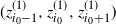$(z_{i_0-1}^{(1)}, z_{i_0}^{(1)}, z_{i_0+1}^{(1)})$ is a split for some $i_0\in \{2,3,\dots, n-1\}$ ; by the definition of split configuration, $i_0$ must be greater than 1 and smaller than n. Accordingly, note that $z_{i_0}^{(1)}$ is negligible and consider the preliminary modification $z^{(1)}\mapsto \hat{z}^{(1)}$ given by

\begin{align*}(\dots, z_{i_0-1}^{(1)}, z_{i_0}^{(1)}, z_{i_0+1}^{(1)}, \dots) \longrightarrow (\dots, z_{i_0-1}^{(1)},0, z_{i_0+1}^{(1)}, \dots),\end{align*}

which changes $z_{i_0}^{(1)}$ into 0 (so $\hat{z}^{(1)}\not\in \mathcal{S}$ : we will handle this later). As $z_{i_0-1}^{(1)}>z_{i_0}^{(1)}$ , we have

(4.7) \begin{equation} \Bigg|\frac{z_{i_0-1}^{(1)}}{z_{i_0-2}^{(1)}+z_{i_0-1}^{(1)}}-\frac{z_{i_0-1}^{(1)}}{z_{i_0-1}^{(1)}+z_{i_0}^{(1)}}\Bigg| < \Bigg|\frac{z_{i_0-1}^{(1)}}{z_{i_0-2}^{(1)}+z_{i_0-1}^{(1)}}-1\Bigg| \end{equation}

if only 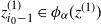${z_{i_0-1}^{(1)}\in \phi_{\alpha}(z^{(1)})}$ . Similarly, as $z_{i_0}^{(1)}<z_{i_0+1}^{(1)}$ , we get

(4.8) \begin{equation} \Bigg|\frac{z_{i_0+1}^{(1)}}{z_{i_0}^{(1)}+z_{i_0+1}^{(1)}}-\frac{z_{i_0+1}^{(1)}}{z_{i_0+1}^{(1)}+z_{i_0+2}^{(1)}}\Bigg| < \Bigg|1-\frac{z_{i_0+1}^{(1)}}{z_{i_0+1}^{(1)}+z_{i_0+2}^{(1)}}\Bigg| \end{equation}

as long as 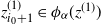${z_{i_0+1}^{(1)}\in \phi_{\alpha}(z^{(1)})}$ . By (4.7) and (4.8), with a slight abuse of notation (the domain of $\Psi_{\alpha}$ does not formally contain $\hat{z}^{(1)}$ , but we may extend the definition for $\Psi_{\alpha}(\hat{z}^{(1)})$ in a straightforward way), we can write $\Psi_{\alpha}(z^{(1)}) \le \Psi_{\alpha}(\hat{z}^{(1)})$ . Now, let us write $\hat{z}^{(1, \leftarrow)} = \big(0, \hat{z}_{1}^{(1)}, \dots, \hat{z}_{i_0-1}^{(1)}, 0\big)$ and $\hat{z}^{(1, \rightarrow)} = \big(0, \hat{z}_{i_0+1}^{(1)}, \dots, \hat{z}_{n}^{(1)}, 0\big)$ . In other words, the sequences $\hat{z}^{(1, \leftarrow)}$ and $\hat{z}^{(1, \rightarrow)}$ are two consecutive parts of $\hat{z}^{(1)}$ and we can restore $\hat{z}^{(1)}$ by glueing their corresponding zeros together. Moreover, after normalising them by the weights $w^{(1,\leftarrow)}=\sum_{i=1}^{i_0-1}\hat{z}_{i}^{(1)}$ and $w^{(1,\rightarrow)}=\sum_{i=i_0+1}^{n}\hat{z}_{i}^{(1)}$ , we get $(w^{(1,\leftarrow)})^{-1}\hat{z}^{(1,\leftarrow)},(w^{(1,\rightarrow)})^{-1}\hat{z}^{(1,\rightarrow)}\in\mathcal{S}$ . Next, in this setup, we are left with

\begin{align*} \Psi_{\alpha}(\hat{z}^{(1)}) & = w^{(1, \leftarrow)}\cdot\Psi_{\alpha}\bigg( \frac{\hat{z}^{(1, \leftarrow)}}{w^{(1, \leftarrow)}}\bigg) + w^{(1, \rightarrow)}\cdot\Psi_{\alpha}\bigg(\frac{\hat{z}^{(1, \rightarrow)}}{w^{(1, \rightarrow)}}\bigg) \\[5pt] & \le \max\bigg\{\Psi_{\alpha}\bigg( \frac{\hat{z}^{(1, \leftarrow)}}{w^{(1, \leftarrow)}}\bigg), \Psi_{\alpha}\bigg(\frac{\hat{z}^{(1, \rightarrow)}}{w^{(1, \rightarrow)}}\bigg)\bigg\}, \end{align*}

where we have used $w^{(1, \leftarrow)}+w^{(1, \rightarrow)}=1$ . Let

\begin{align*} \tilde{z}^{(1)} = \arg\max\bigg\{\Psi_{\alpha}(z)\colon z \in \bigg\{\frac{\hat{z}^{(1,\leftarrow)}}{w^{(1,\leftarrow)}},\frac{\hat{z}^{(1,\rightarrow)}}{w^{(1,\rightarrow)}}\bigg\}\bigg\}. \end{align*}

By construction, we have $\Psi_{\alpha}(z^{(1)}) \le \Psi_{\alpha}(\tilde{z}^{(1)})$ , the new sequence $\tilde{z}^{(1)}$ is shorter than $z^{(1)}$ , and $\tilde{z}^{(1)}$ contains fewer split configurations than $z^{(1)}$ . After repeating this procedure ( $z^{(1)}\mapsto \tilde{z}^{(1)}$ ) multiple times, we acquire a new sequence $z^{(2)}$ obeying requirements (1) and (2).

$z^{(2)} \rightarrow z^{(3)}$ . Surprisingly, it is enough to put $z^{(3)}=z^{(2)}$ . Indeed, we can show that the sequence $z^{(2)}$ already satisfies the third condition. First, suppose that 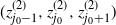$(z_{j_0-1}^{(2)},z_{j_0}^{(2)},z_{j_0+1}^{(2)})$ and 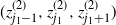$(z_{j_1-1}^{(2)}, z_{j_1}^{(2)}, z_{j_1+1}^{(2)})$ are two different peaks with indices $j_0<j_1$ . Hence, as $z_{j_0}^{(2)}>z_{j_0+1}^{(2)}$ and $z_{j_1-1}^{(2)}<z_{j_1}^{(2)}$ , there is at least one point $i_0\in\{j_0+1, \dots, j_1-1\}$ at which we are forced to ‘flip’ the direction of the previous inequality sign:

\begin{align*}z_{j_0-1}^{(2)}< z_{j_0}^{(2)}>z_{j_0+1}^{(2)}>\dots > z_{i_0}^{(2)}<\dots<z_{j_1-1}^{(2)}< z_{j_1}^{(2)}>z_{j_1+1}^{(2)}.\end{align*}

Equivalently, this means that 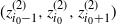$(z_{i_0-1}^{(2)}, z_{i_0}^{(2)}, z_{i_0+1}^{(2)})$ is a split configuration. This contradicts our initial assumptions about $z^{(2)}$ (requirement (2) is not met) and proves that there is at most one peak in $z^{(2)}$ . Second, we have $0=z_{0}^{(2)}<z_1^{(2)}$ and 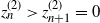$z_{n}^{(2)}>z_{n+1}^{(2)}=0$ , so there exists a point $j_0$ at which the direction of the inequalities must be changed from ‘ $<$ ’ to ‘ $>$ ’. Thus, there is at least one peak in $z^{(2)}$ .

$z^{(3)} \rightarrow z^{(4)}$ . Let $z^{(3)}=(z_i^{(3)})_{i=0}^{n+1}$ and assume that 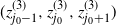$(z_{j_0-1}^{(3)}, z_{j_0}^{(3)}, z_{j_0+1}^{(3)})$ is the unique peak of $z^{(3)}$ :

(4.9) \begin{equation} 0<z_1^{(3)}<\dots<z_{j_0-1}^{(3)} < z_{j_0}^{(3)} > z_{j_0+1}^{(3)} > \dots > z_n^{(3)}>0. \end{equation}

The further reasoning is similar to points (1) and (2), so we will just sketch it. If requirement (4) is not satisfied, pick a negligible component $z_{i_0}^{(3)}$ with $i_0\not=j_0$ . Next, apply the transformation $z^{(3)}\mapsto\tilde{z}^{(3)}$ defined by (4.6), i.e. remove $z_{i_0}^{(3)}$ and rescale the remaining components. Thanks to the ‘single-peak structure’ (4.9), all the significant components of $z^{(3)}$ remain significant for $\tilde{z}^{(3)}$ . The terms associated with components $z^{(3)}_i \in \phi_{\alpha}(z^{(3)})\setminus \{z_{i_0-1}^{(3)}, z_{i_0+1}^{(3)} \}$ are not changed (and their contribution grows after the rescaling). The summands corresponding to $z_{i_0-1}^{(3)}$ and $z_{i_0+1}^{(3)}$ can only increase, just as in (4.7) and (4.8). Therefore $\Psi_{\alpha}(z^{(3)}) \le \Psi_{\alpha}(\tilde{z}^{(3)})$ . After several repetitions and discarding of all unnecessary negligible components (beyond the central $z_{j_0}$ ), we finally obtain the desired sequence $z^{(4)}\in \mathcal{S}'$ .

We proceed to the proof of our main result.

Proof of Theorem 1.3. We start with the lower estimate, for which the argument is simpler. By Proposition 4.3 and the reformulation in (4.5), for $\alpha > 2$ ,

\begin{align*} \alpha\cdot\sup_{(X,Y)\in\mathcal{C}}\mathbb{E}|X-Y|^{\alpha} = \alpha\cdot\sup_{z\in\mathcal{S}}\Phi_{\alpha}(z) & \ge \alpha\cdot\Phi_{\alpha}\bigg(0,\frac{1}{\alpha},\frac{\alpha-2}{\alpha},\frac{1}{\alpha},0\bigg) \\[5pt] & = \alpha\cdot\frac{2}{\alpha}\bigg|1-\frac{1}{\alpha-1}\bigg|^{\alpha} \xrightarrow{\alpha\rightarrow\infty} \frac{2}{\mathrm{e}}. \end{align*}

Now we turn our attention to the upper estimate. By Propositions 4.4 and 4.5, we get

\begin{align*} \alpha\cdot\sup_{(X,Y)\in\mathcal{C}}\mathbb{E}|X-Y|^{\alpha} \le \alpha\cdot\bigg(\bigg|1-\frac{1}{1+\sqrt{\alpha}\,}\bigg|^{\alpha} + \sup_{z\in\mathcal{S}'}\Psi_{\alpha}(z)\bigg). \end{align*}

Next, because

\begin{align*}\lim_{\alpha \to \infty} \alpha\cdot \bigg|1-\frac{1}{1+\sqrt{\alpha}\,}\bigg|^{\alpha} = 0,\end{align*}

it is enough to provide an asymptotic estimate for $\alpha\cdot\sup_{z\in\mathcal{S}'}\Psi_{\alpha}(z)$ . Fix an arbitrary $z= (z_0, z_1,\dots, z_{n+1})\in \mathcal S'$ and let $z_{j_0}$ be the centre of the unique peak contained in z:

\begin{align*}0<z_1<\dots<z_{j_0-1} < z_{j_0} > z_{j_0+1} > \dots > z_n>0.\end{align*}

As $z_{j_0}$ is the only negligible component contained in z, we have $\sqrt{\alpha}\cdot z_i<z_{i+1}$ for $1\le i\le j_{0}-1$ and $z_{i-1}>\sqrt{\alpha}\cdot z_i$ for $j_0+1\le i\le n$ . In particular, we get $0\le z_{j_0-1}, z_{j_0+1} < 1/\sqrt{\alpha}$ . Consequently, we can write $\Psi_{\alpha}(z) = A + B + C$ , where

\begin{align*} A & = \sum_{|i-j_0|>2}z_i\bigg|\frac{z_i}{z_{i-1}+z_i} - \frac{z_i}{z_i+z_{i+1}}\bigg|^{\alpha}, \\[5pt] B & = z_{i_0-2}\bigg|\frac{z_{i_0-2}}{z_{i_0-3} + z_{i_0-2}} - \frac{z_{i_0-2}}{z_{i_0-2} + z_{i_0-1}}\bigg|^{\alpha} + z_{i_0+2}\bigg|\frac{z_{i_0+2}}{z_{i_0+1} + z_{i_0+2}} - \frac{z_{i_0+2}}{z_{i_0+2} + z_{i_0+3}}\bigg|^{\alpha}, \\[5pt] C & = z_{i_0-1}\bigg|\frac{z_{i_0-1}}{z_{i_0-2} + z_{i_0-1}} - \frac{z_{i_0-1}}{z_{i_0-1} + z_{i_0}}\bigg|^{\alpha} + z_{i_0+1}\bigg|\frac{z_{i_0+1}}{z_{i_0} + z_{i_0+1}} - \frac{z_{i_0+1}}{z_{i_0+1} + z_{i_0+2}}\bigg|^{\alpha}. \end{align*}

We examine these three parts separately.

Looking at A, since $z_i/(z_{i-1}+z_i)$ and $z_{i}/(z_i+z_{i+1})$ belong to [0, 1], we may write

\begin{align*} A \le \sum_{i=1}^{j_0-3}z_i + \sum_{i=j_0+3}^{n}z_i & < z_{j_0-3}\cdot\sum_{i=0}^{j_0-4}\bigg(\frac{1}{\sqrt{\alpha}\,}\bigg)^i + z_{j_0+3}\cdot\sum_{i=0}^{n-j_0-3}\bigg(\frac{1}{\sqrt{\alpha}\,}\bigg)^i \\[5pt] & < (z_{j_0-1}+z_{j_0+1})\cdot\frac{1}{\alpha}\cdot\sum_{i=0}^{\infty}\bigg(\frac{1}{\sqrt{\alpha}\,}\bigg)^i \\[5pt] & < \frac{2}{\alpha\sqrt{\alpha}\,}\cdot\sum_{i=0}^{\infty}\bigg(\frac{1}{\sqrt{\alpha}\,}\bigg)^i = \frac{2}{\alpha(\sqrt{\alpha}-1)}, \end{align*}

and hence

\begin{align*}\alpha\cdot A < \frac{2}{\sqrt{\alpha}-1} \xrightarrow{\alpha \rightarrow \infty} 0.\end{align*}

For B, we have

\begin{align*} B & \le z_{i_0-2}\bigg|1-\frac{z_{i_0-2}}{z_{i_0-2} + z_{i_0-1}}\bigg|^{\alpha} + z_{i_0+2}\bigg|\frac{z_{i_0+2}}{z_{i_0+1} + z_{i_0+2}}-1\bigg|^{\alpha} \\[5pt] & < z_{i_0-2}\bigg|1-\frac{z_{i_0-2}}{z_{i_0-2} + ({1}/{\sqrt{\alpha}})}\bigg|^{\alpha} + z_{i_0+2}\bigg|\frac{z_{i_0+2}}{({1}/{\sqrt{\alpha}}) + z_{i_0+2}}-1\bigg|^{\alpha} \\[5pt] & \le 2\cdot\sup_{x\in[0,1]}x\bigg|1-\frac{x}{x+({1}/{\sqrt{\alpha}})}\bigg|^{\alpha} = \frac{2}{\sqrt{\alpha}(\alpha-1)}\cdot\bigg(1-\frac{1}{\alpha}\bigg)^{\alpha}. \end{align*}

This yields

\begin{align*}\alpha\cdot B < \frac{2\sqrt{\alpha}}{\alpha-1}\cdot\bigg(1-\frac{1}{\alpha}\bigg)^{\alpha} \xrightarrow{\alpha \rightarrow \infty} 0.\end{align*}

Finally, for C, we observe that

\begin{align*} C & \le z_{i_0-1}\bigg|1-\frac{z_{i_0-1}}{z_{i_0-1} + z_{i_0}}\bigg|^{\alpha} + z_{i_0+1}\bigg|\frac{z_{i_0+1}}{z_{i_0} + z_{i_0+1}}-1\bigg|^{\alpha} \\[5pt] & \le z_{i_0-1}|1-z_{i_0-1}|^{\alpha} + z_{i_0+1}|z_{i_0+1}-1|^{\alpha} \\[5pt] & \le 2\cdot\sup_{x\in[0,1]}x|1-x|^{\alpha} = \frac{2}{\alpha+1}\cdot\bigg(1-\frac{1}{\alpha+1}\bigg)^{\alpha}. \end{align*}

Consequently, we obtain

\begin{align*}\alpha\cdot C \le \frac{2\alpha}{\alpha+1}\cdot\bigg(1-\frac{1}{\alpha+1}\bigg)^{\alpha} \xrightarrow{\alpha \rightarrow \infty} \frac{2}{\mathrm{e}}.\end{align*}

The estimates for A, B, and C give the desired upper bound. The proof is complete.

5. Concluding remarks

The proof of Theorem 1.3 presented above is just an example of a novel, geometric-type approach in the analysis of coherent distributions and related inequalities. We strongly believe that our study of extreme coherent distributions will turn out to be useful in other applications. While some of the results obtained can be easily extended to a wider context, others seem to be harder to generalize. Let us include a short discussion.

• Definition 1.1, Proposition 1.1, and Theorem 1.4 extend naturally to higher dimensions—the omitted proofs remain analogous. For an arbitrary number $n\ge2$ , extreme coherent distributions on $[0,1]^n$ are exactly those whose representations are unique and minimal.

• It is unclear whether Theorem 3.1 enjoys any comparable counterpart for $n\ge3$ . Without resolving this open question, plausible applications of our geometric approach are rather limited to the two-variate setup.

• A stronger result follows immediately from the proof of Proposition 4.2. We have

  \begin{align*}\sup_{(X,Y)\in\mathcal{C}}\mathbb{E}\tilde{f}(X,Y) = \sup_{(X,Y)\in\mathrm{ext}_\mathrm{f}(\mathcal{C})}\mathbb{E}\tilde{f}(X,Y)\end{align*}
  for every continuous function $\tilde{f}\colon[0,1]^2\rightarrow[0,1]$ .

• The converse of Theorem 3.1 does not hold true. For example, let m be a probability distribution given by

  \begin{align*}m\bigg(\frac{1}{4}, 0\bigg) = \frac{1}{3}, \qquad m\bigg(\frac{1}{4}, \frac{3}{4}\bigg) = \frac{1}{3}, \qquad m\bigg(1, \frac{3}{4}\bigg) = \frac{1}{3}.\end{align*}
  The support of m is just a three-point axial path without cycles. Next, the unique representation of m is now clearly determined by the quotient function
  \begin{align*}q\bigg(\frac{1}{4}, 0\bigg)=0, \qquad q\bigg(\frac{1}{4}, \frac{3}{4}\bigg) = \frac{1}{2}, \qquad q\bigg(1, \frac{3}{4}\bigg) = 1.\end{align*}
  Note that $(\frac{1}{4}, \frac{3}{4})$ is a cut point, even though it is not an endpoint of the axial path. Thus, by Corollary 3.1, coherent measure m is not an extreme point. Indeed, we have $m = \frac{1}{2}(m_1+m_2)$ , where $m_1, m_2 \in \mathcal{C}$ are given by
  \begin{align*}m_1\bigg(\frac{1}{4}, 0\bigg) = \frac{2}{3}, \qquad m_1\bigg(\frac{1}{4}, \frac{3}{4}\bigg) = \frac{1}{3}, \qquad m_2\bigg(\frac{1}{4}, \frac{3}{4}\bigg) = \frac{1}{3}, \qquad m_2\bigg(1, \frac{3}{4}\bigg) = \frac{2}{3}.\end{align*}
  In practice, to prove the extremality of a discrete coherent distribution (whose support is an axial path without cycles), we need to compute its quotient function.

• In the proof of Proposition 4.3, we applied Corollary 3.1 to justify the reduction (1.1). A similar argumentation might enable or simplify the evaluation of the quantity $\sup_{(X,Y)\in\mathrm{ext}_\mathrm{f}(\mathcal{C})}\mathbb{E}\tilde{f}(X,Y)$ for multiple (not necessarily convex) continuous functions $\tilde{f}\colon[0,1]^2\rightarrow[0,1]$ .