Ice physics and its development over the last half century is not easy to tackle in 45 minutes. In 1974, Peter Hobbs published a book with the title Ice physics that had 835 pages. Most of the work he summarized was done in the period under review. Ice physicists have got together at conferences at various times. The first, at Erlenbach in Switzerland in 1962 was quite a small affair. Another, in Sapporo in 1966 (Reference ŌuraŌura, 1967), covered more applied aspects. Munich in 1968 (Reference Riehl, Riehl, Bullemer and EngelhardtRiehl and others, 1969) was followed by the institution of an informal international committee which has arranged for further conferences in Ottawa in 1972 (Reference Whalley, Whalley, Jones and GoldWhalley and others, 1973), Cambridge in 1977 (Reference Hayes and WebbGlen and others, 1978), Rolla in 1982 (Reference El-SayadEl-Sayed, 1983), and Grenoble in 1986. The last in this series occurred last week [September 1986] and will be published in 1987 in Journal de Physique Collogues. Each of these conferences has had many papers over a wide range of ice physics and the volumes resulting from them give an impressive overview of the amount of work which has been done – and the impossibility of summarizing it properly in this lecture. Thus, what I include will be largely a subjective view of what seem to be the most interesting developments in ice physics – in our basic understanding of the physics underlying the behaviour of our material, ice, which is the link between all the geophysical phenomena discussed in the other lectures.

Ice is a very interesting and important material, not only to the glaciologist but also to meteorologists and geologists, physicists and chemists, astronomers and biologists. The physical properties of ice are interesting and unusual, and are responsible for behaviour that has allowed life to develop on Earth – the unusual (but not unique) situation where the solid is less dense than the liquid allows water bodies to survive under an insulating cover of ice and so preserve the marine life underneath. This, of course, is one physical property of ice that has been known for a very long time, but another very important peculiarity of ice had only just been appreciated 50 years ago at the time the International Glaciological Society was founded, and much of the most interesting ice physics has come from studying the consequences. This is the strange situation of the locations of the hydrogen atoms in ice.

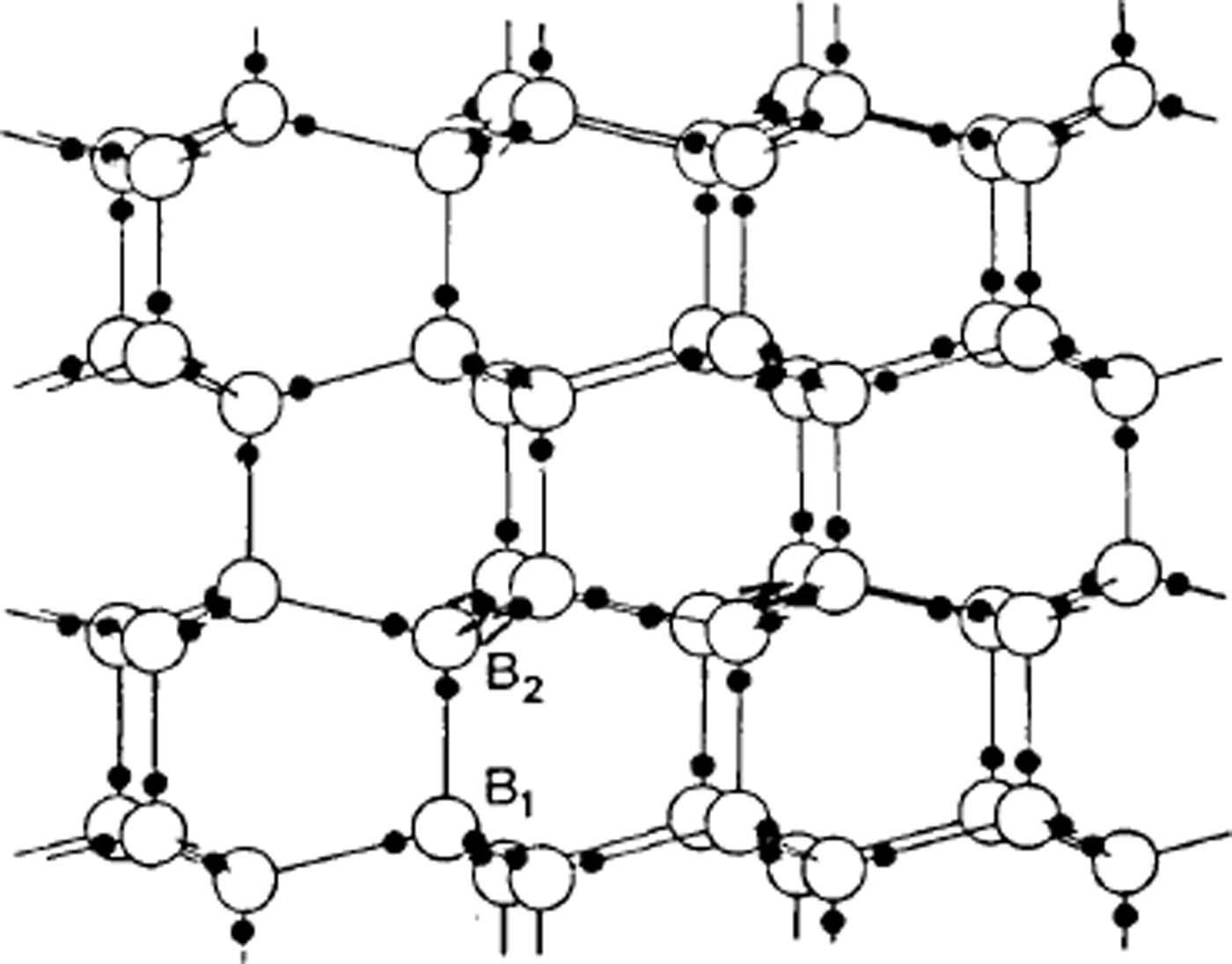
One of the first applications of X-ray crystallography was to determine the structure of ice. In 1921, Reference BraggBragg (1921) interpreted measurements by Reference DennisonDennison (1921) to show that the oxygen atoms were arranged tetrahedrally to form the hexagonal structure we call ice Ih. However, X-rays do not readily locate very light atoms, and the position of the hydrogens is not indicated by the experimental data. Bragg supposed they were half-way between the oxygen atoms, but Reference Bernal and FowlerBernal and Fowler (1933) suggested, more plausibly, that two hydrogens were near to each oxygen atom so that every bond had one hydrogen on it and every oxygen had two hydrogens near it, so that water molecules are preserved in the structure. In this model each water molecule is essentially a nearly spherical object with the hydrogen nuclei, two to each molecule, being small centres of positive charge (protons) partly compensated by concentrations of electron distribution, while two other concentrations of electron distribution give two centres of negative charge. In the structure the positive centres of one water molecule are electrostatically attracted to the negative centres of the neighbouring water molecules. To account for the fact that ice is not observed to be polar in its properties, a very large unit cell would be needed if the hydrogens were to be regularly arranged, but thermal measurements suggested that ice Ih had some built-in disorder, and Reference PaulingPauling (1935) suggested that this might be due to the hydrogen atoms being disordered; in other words, if we know where one hydrogen atom is, we do not automatically know where corresponding hydrogens are in a neighbouring, crystallographically equivalent part of the ice structure – ice is a crystal as regards the oxygens but a glass as regards the hydrogens (Fig. 1).

Fig. 1.

The arrangement of water molecules in ice Ih. Note that the three water molecules bonded to B₂ are vertically above those bonded to B₁. The hydrogen atoms are shown in positions consistent with the Bernal-Fowler rules.

This, then, was the understanding of the basic physics of ice that had been achieved 50 years ago, but the way in which this unusual feature of random hydrogen positions was related to the macroscopic properties of ice was still to be worked out. The problem can perhaps best be understood by considering what happens when ice is put in an electric field. In fact, in such an experiment the ice becomes polarized and the dipole moment per water molecule produced is of the same order of magnitude as it is for liquid water. Now, this is really a very surprising result. In liquid water it is obvious that individual water molecules, which, as we have seen, have centres of positive and negative charge within them, can be expected to rotate in such a way that the energy of the dipole is lowered — they align themselves with the electric field. Since ice produces about the same dipole moment, this means that in ice, too, water molecules align themselves with the field – but how can they do this? Even if the hydrogens are random, any individual water molecule has four neighbours, two of which present negative charges to it and two of which present positive charges, so the orientation of the water mole.cule is completely determined and it cannot turn round unless its neighbours turn as well. Indeed, if the Bernal and Fowler structure with Pauling's randomness were the whole story, ice ought to be much less polarizable than water.

The solution was found by Reference BjerrumBjerrum (1951), who suggested that the two rules for the structure suggested by Reference Bernal and FowlerBernal and Fowler (1933) (and now known as the Bernal- Fowler rules) may occasionally be breached and that the defects resulting from breaching these rules allow ice molecules to re-orient. One of the rules states that each oxygen has two hydrogens, that is to say we are dealing with water molecules. Now, it is well known that in water this rule is occasionally breached – water is weakly ionized and according to the chemical law of mass action has in equilibrium a small number of H₃O⁺ and OH⁻ ions

It is this small number of ions that allows water to conduct electricity and their number is assessed in logarithmic form by the so-called pH. Thus, it is surely to be expected that in ice too a very small number of oxygens will have three or one hydrogen instead of two. Now, if this is so, Bjerrum pointed out that hydrogen atoms could move from one molecule to another (Fig. 2a and b) – if one of the three hydrogens of an H₃O⁺ ion moves along its bond to the neighbouring molecule, then that molecule becomes the ion. If now another hydrogen of the new molecule moves away, a third molecule has become the ion and the molecule through which the ion has passed has been reoriented. Thus, a mechanism is found for re-orienting water molecules, and it would work equally well for an OH⁻ ion. Note that, unlike the case in water, the oxygens have not moved at all, the charge movement is entirely due to protons (hydrogen nuclei) moving along bonds.

Fig. 2.

The creation and movement of electrical point defects in ice. In (a) the movement of a proton from the position shown with a dashed circle creates a positive and a negative ion, and (b) shows how movements of a proton along a bond can make the ions migrate, (c) shows how the movement of a proton around an oxygen atom can create an L-defect and a D-defect, and (d) shows how this defect can also migrate by further movements of protons around oxygen atoms. The movement of the protons is to the right in all cases, but the movement of ions in (b) leaves the water molecules oriented with their protons to the left, while the movement of L- and D-defects in (d) leaves them with their protons to the right.

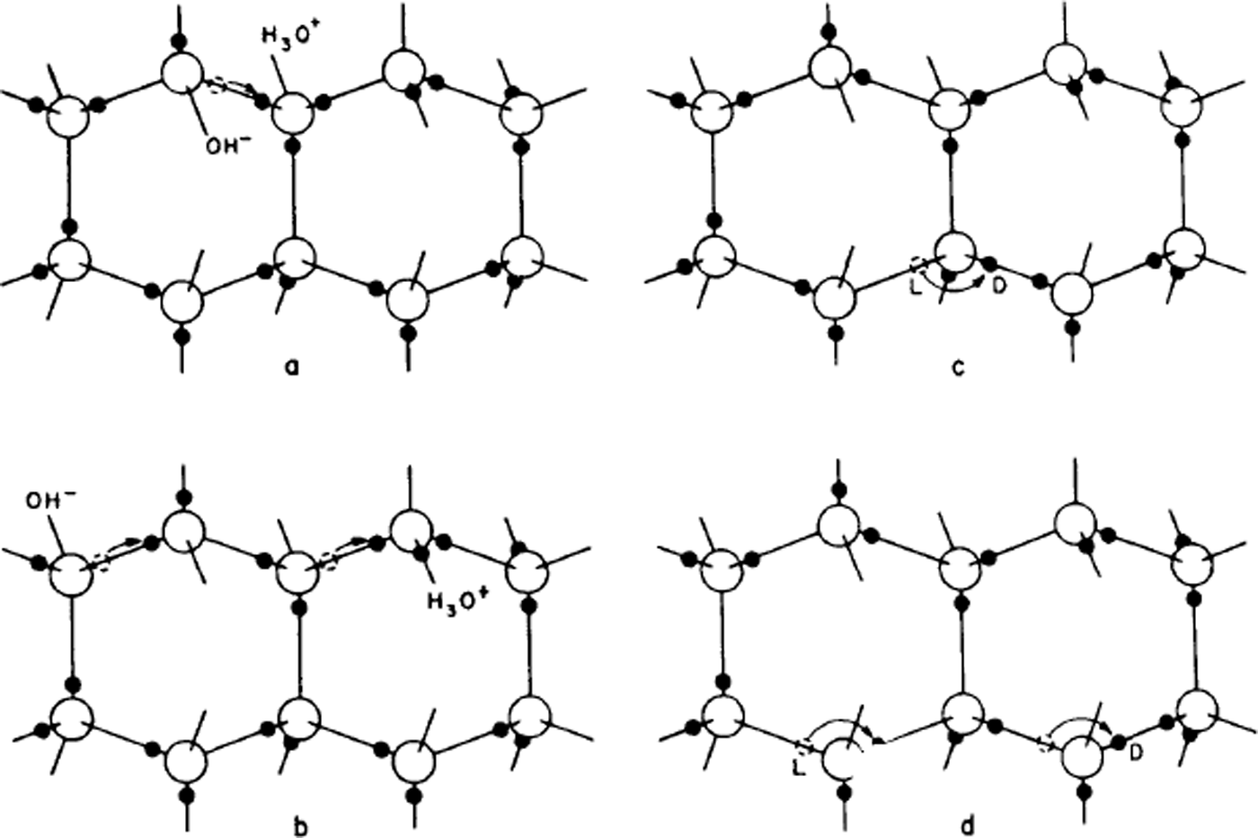
The second Bernal–Fowler rule states that there is one hydrogen per bond. If we now suppose that this too is breached for a small number of bonds, we get other sorts of point defect, now known as Bjerrum defects. A bond with no hydrogens on it is called an L-defect (from the Danish word leer for empty), one with two hydrogens is called a D-defect (doppelt or double).

Just as in the case of ionic defects, the Bjerrum defects can move through the structure and cause water molecules to rotate (Fig. 2c and d), only this time the process is one in which protons (hydrogen nuclei) move from one bond to another on the same water molecule. In this case, it is even more obvious that the water molecule is rotated by the process.

In fact, any one sort of defect could cause ice to polarize in an electric field, while if both ions and Bjerrum defects are present, protons can move large distances in the ice; in other words, ice can conduct a direct current. They move along a bond by the passage of an ionic defect and from one bond to another by the passage of a Bjerrum defect. In this way, Bjerrum's ideas can explain both the dipole moment (i.e. the dielectric permittivity) of ice and also the small d.c. conductivity of ice.

The full implications of this for the electrical properties of ice have been the subject of much experiment and theory throughout the half century we are considering. The possibility of using ice doped with HF was exploited first by the Zurich group under Granicher, and the resulting theory was developed by Reference JaccardJaccard (1959, Reference Jaccard1964) and refined by Reference HubmannHubmann (1979). Experiments are not particularly easy to perform, especially when the d.c. conductivity is to be studied, because the current is being carried by protons whereas most electrical circuits consist of conductors for electrons, so that space charges can build up in the ice and prevent proper measurements unless special contacts exist (protodes!) which will give out or receive protons. Work to develop such contacts was done by the group in Grenoble using ion-exchange membranes (Reference Kahane, Riehl, Riehl, Bullemer and EngelhardtKahane, 1969) and ionized hydrogen gas (Reference Auvert, Kahane, Whalley, Whalley, Jones and GoldAuvert and Kahane, 1973), and also by the group in Munich using hydrogen-loaded palladium (Reference Engelhardt and RiehlEngelhardt and Riehl, 1965, Reference Engelhardt and Riehl1966). This latter technique was further refined by Petrenko during a sabbatical visit to Birmingham (Reference Petrenko, Petrenko, Whitworth and GlenPetrenko and others, 1983) and has been used by him to inject protons into ice and study space-charge limited currents. These experiments have served to provide experimental values for the energies required to produce and move the different kinds of defects, and to give a reasonable theoretical background for understanding the electrical properties of ice.

These properties are of great importance for understanding not only the behaviour of ice in a static electric field such as is used in resistivity sounding of glaciers, but also in alternating fields including those provided by electromagnetic waves. As the frequency increases, so the ability of water molecules to rotate decreases and a typical relaxation process occurs (Fig. 3). This was first studied in detail for polycrystalline ice by Reference Auty and ColeAuty and Cole (1952), who showed that pure ice is really a very good example of a relaxation process in a dielectric. At the higher frequencies used in radio echo-sounding, ice has very little absorption; that is to say, the dipole polarization is essentially in phase with the applied field, but the existence of reflection horizons implies relatively sudden changes in the dielectric permittivity of the ice that have puzzled glaciologists since their discovery. The electrical properties are also of much interest to cloud physicists, since ideas of the origin of thunderstorm electricity are related to various electrical phenomena of ice crystals.

Fig. 3.

Plot of the real and imaginary parts of the permittivity of ice (the so-called Cole-Cole plot). The three plots are for different temperatures as marked; the two curves on each plot are for measurements parallel and perpendicular to the c-axis. The plots are almost perfect semi-circles. The deviations at the right of the top plot are due to the effect of electrical conductivity. The frequencies in kHz are marked against points. (After Reference Humbel, Humbel, Jona and ScherrerHumbel and others, 1953.)

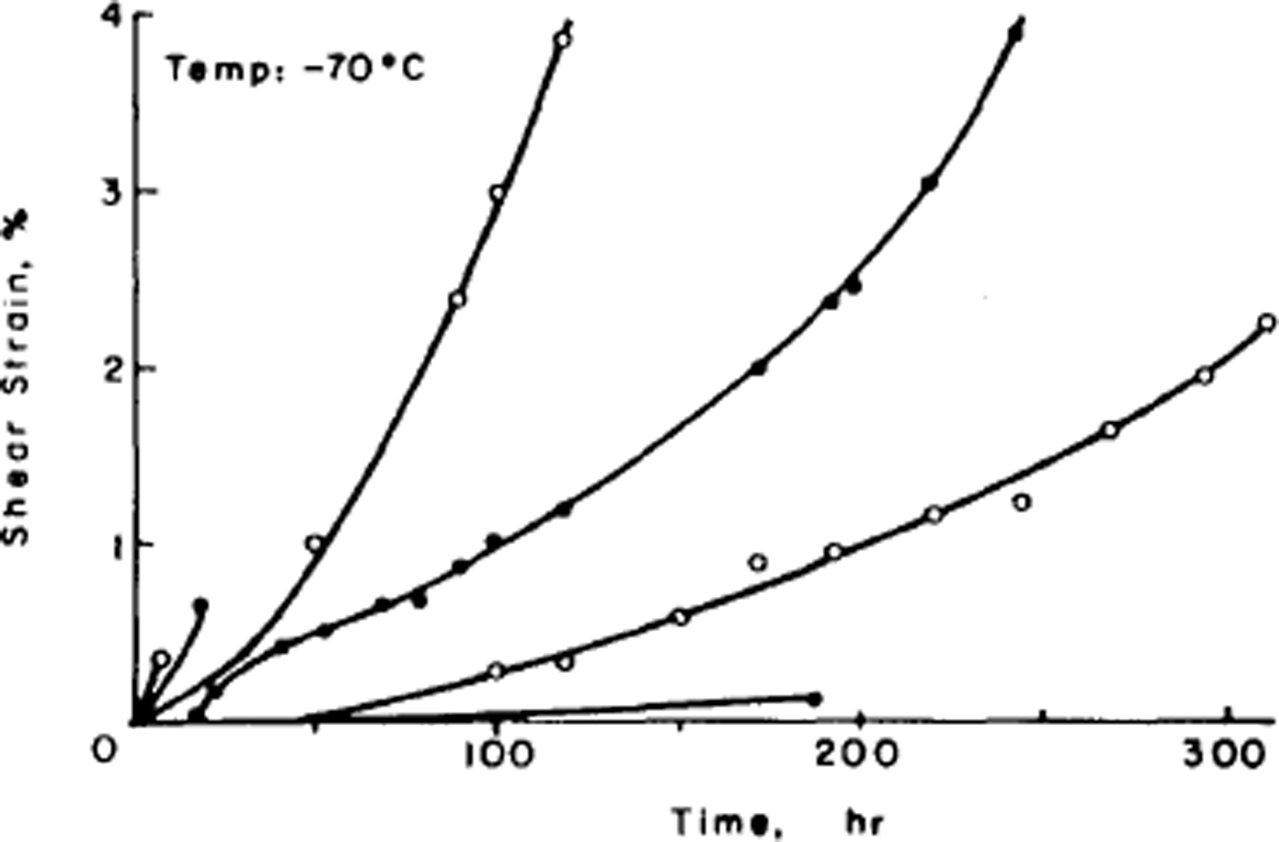
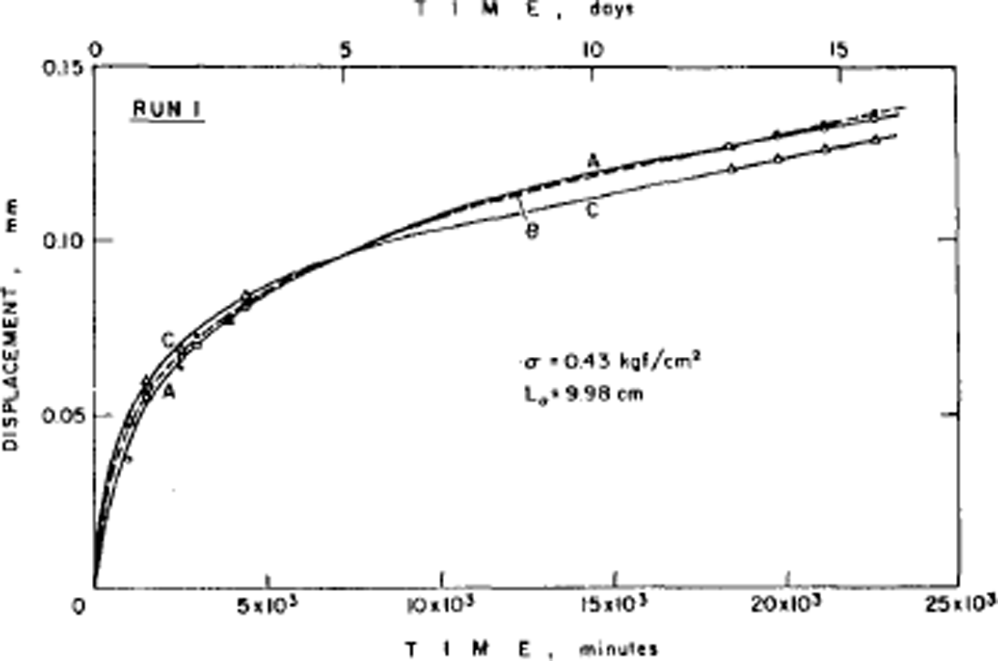
The disorder of the hydrogen atoms in ice also poses problems for understanding the mechanical properties of ice. Early experiments had shown that ice single crystals deform easily only by slip on the (0001) or basal planes and consequently polycrystalline ice is much harder to deform than single crystals. The physical explanation of ice deformation had thus first to understand why ice deforms easily only on the basal plane and to discover what limits the deformation on that plane, and then had to see how crystals of different orientation interact to produce the creep properties (flow law) of polycrystalline ice. Experiments by the present author had established (Reference Hamilton, Hamilton, Kamb, LaPlaca, Prakash, Riehl, Riehl, Bullemer and EngelhardtGlen and Perutz, 1954) that single crystals have accelerating creep curves (Fig. 4), while (Reference GlenGlen, 1955) polycrystalline ice had decelerating creep curves (Fig. 5) whose steady-state creep was related to stress by a power law. Since ice is crystalline, we would expect these properties to result from the ability of dislocations to move through the ice, impeded either by the force required to make the dislocations move at all or by the force of interaction between dislocations. However, the same disorder of the hydrogen atoms introduces a major difficulty here since, when a crystal deforms by movement of dislocations, the molecules break a bond with one partner and remake it with another. If one of these molecules has a hydrogen at the top of a bond, it can only remake the bond with a molecule so oriented as to have no hydrogen at the bottom of the bond, and with randomized bond orientations this will frequently not be the case (Reference GlenGlen, 1968) (Fig. 6). Thus, there is a problem about dislocation movement in ice that is peculiar to a material with this kind of randomness, and there is therefore great interest in measuring the velocity with which dislocations move through ice and comparing the results with theories, and also for seeing whether dislocations can in fact move on non-basal planes. A good method for achieving this is to use X-ray topography which in principle allows us to see dislocations in ice. The first successful use of this technique in ice was reported by Reference Hayes and WebbHayes and Webb (1965) and it has been used by groups in Sapporo (Reference Fukuda, Higashi, Riehl, Riehl, Bullemer and EngelhardtFukuda and Higashi, 1969, Reference Fukuda and Higashi1973) and Villeurbanne (Reference MaïMai, 1976) to deduce dislocation velocities. The observed velocities are such that it is difficult to account for them theoretically on a model in which bonds have to be re-oriented by the mechanisms discussed above (Reference WhitworthWhitworth, 1978, Reference Whitworth1983). In Birmingham, we are currently doing experiments using the synchrotron radiation source so that exposure times for X-ray topographs are much reduced and more direct dynamical experiments are possible.

Fig. 4.

Creep curves of ice single crystals deformed under various stresses at –70 C. (After Reference Jones and GlenJones and Glen, 1969.)

Fig. 5.

Low-stress creep curves for fine-grained ice whose crystal orientation was initially random. Test temperature –2.06 C. Constant axial compressive stress of 0.42 bar on ice which had not been previously loaded. (After Reference Mellor and TestaMellor and Testa, 1969.)

Fig. 6.

The effect of moving a dislocation through the ice Ih structure. The top diagram shows a part of the structure with the protons (black circles) at random consistent with the Bernal–Fowler rules. The middle diagram shows the same structure after the top has sheared to the right relative to the bottom by the passage of a dislocation. Note that this has introduced L- and D-defects. An intermediate stage between these two conditions is shown in the bottom diagram where the dislocation is at a position where it has already moved atom A to join B'. Atom B has a dangling bond and. for the dislocation to move on, it must link to C. However, it already has a proton on its bond, and to avoid making a D-defect the proton above C must move away, e.g. to the other end of its bond by the passage of a mobile ion, or around C by the passage of a mobile L-defect.

The effect of the different orientations of single crystals on a polycrystalline aggregate and the difference in flow rate to be expected for ice with different preferred orientations were considered by Reference LileLile (1978), although a detailed study based on the non-basal mechanisms, and grain-boundary migration and sliding, has not been attempted because of the continuing lack of basic information on these processes.

Fifty years ago only the structure of ice Ih was known; however, it was known from the work of Reference TammannTammann (1900) that at high pressures and various temperatures ice could be converted into one of two denser phases, and that these denser phases could be retained at low pressure if they were held at liquid-air temperatures. This work was extended by Reference BridgmanBridgman (1935) who found two further phases of H₂O ice and one additional phase for D₂O ice, and later (Reference BridgmanBridgman, 1937) extended his work to still higher pressures, obtaining yet another phase (Fig. 7). Bridgman noticed that the boundary line on the phase diagram between ice VI and VII appeared to change the angle it makes with the temperature axis near 0 °C and this, and the similar divergence of the boundaries of ice II, suggest that these phases have lower entropy than their neighbours. Reference Whalley, Whalley, Heath and DavidsonWhalley and others (1968) suggested that this means the phases have proton ordering (the ordered form of ice VII they called ice VIII), and this has subsequently been confirmed by other measurements. Similarly, Whalley's group identified a proton-ordered form of ice III that they called ice IX. Much work was done by this group and also by Kamb (Reference Kamb and DattaKamb and Datta, 1960; Reference KambKamb, 1964, Reference Kamb1965; Reference Kamb and DavisKamb and Davis, 1964; Reference Kamb, Kamb, Prakash and KnoblerKamb and others, 1967; Reference Hamilton, Hamilton, Kamb, LaPlaca, Prakash, Riehl, Riehl, Bullemer and EngelhardtHamilton and others, 1969; Reference Engelhardt and KambEngelhardt and Kamb, 1978) to find the crystal structures of these high-pressure ices and some of these are shown in Figures 8–12. All of them have hydrogen bonds similar to those in ice Ih with four molecules bonded to each water molecule, but with different angles and different numbers of molecules in the rings. At the highest pressures, ices VI, VII, and VIII are interesting structures. In order to get the necessary density with only four bonded neighbours, the structures consist of two interpenetrating parts. In the case of ice VII (and VIII) these are both simple structures similar to ice Ih but with the face-centred cubic symmetry of diamond or germanium. Finally, it has been hypothesized that at even higher pressures the hydrogen bonds would eventually get so squashed that ice would have the hydrogen in the middle of the bond – ice X (Reference Hirsch and HolzapfelHirsch and Holzapfel, 1986).

Fig. 7.

Phase diagram of ice. Dashed lines are extrapolated or calculated boundaries. Metastable phases (apart from ice IV and Ic) are shown by light lines. (After Reference Whalley, Whalley, Heath and DavidsonWhalley and others, 1968.)

Fig. 8.

The structure of ice II. The heights of atoms above a hexagonal plane are given in hundredths of the c dimension of the unit cell. One six-ring of each type is emphasized. Note that in the top ring the protons are anti-clockwise from the oxygen atoms and radial, whereas in the lower they are anti-clockwise and alternately up and down. (After Reference KambKamb, 1964.)

Fig. 9.

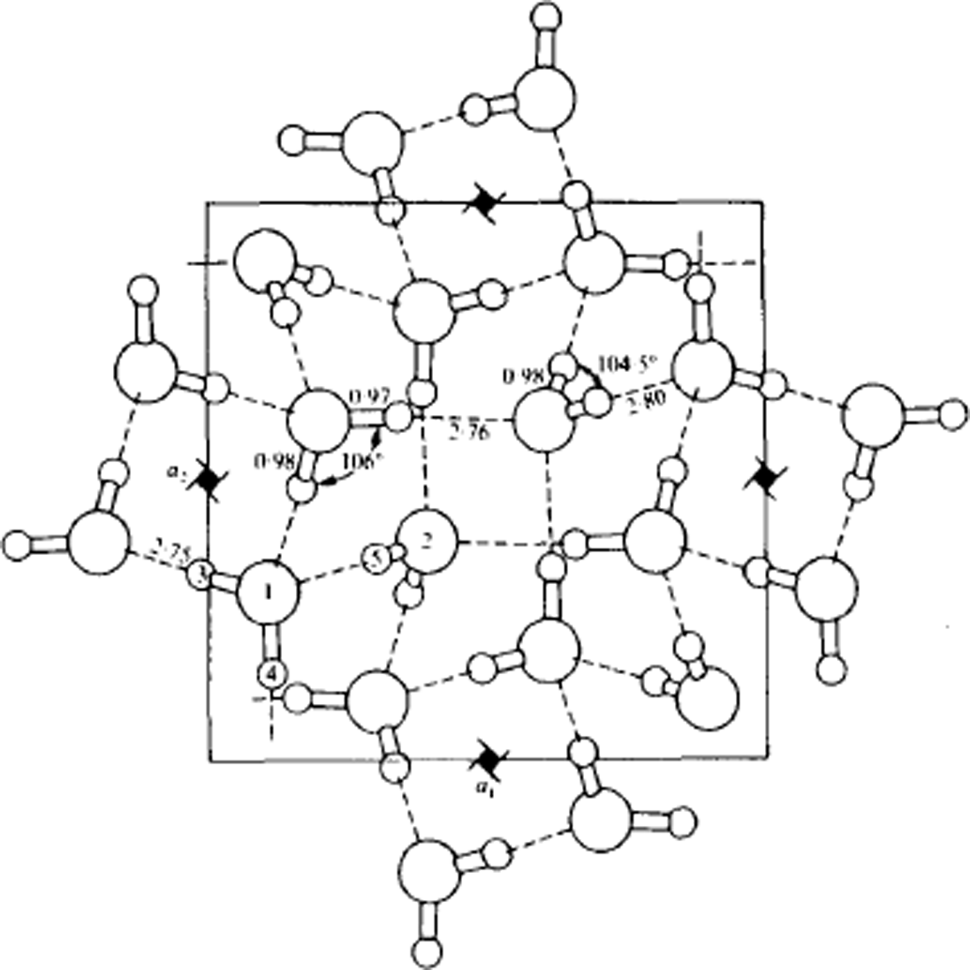
Structure of ice IX, viewed along the tetragonal c-axis. Lengths are in Å. Water molecules of type 1 form helical chains around the 4₁-axes parallel to the c-axis. These helices are linked together laterally by molecules of type 2. If the protons were disordered, the structure would be ice III. (After Reference Hamilton, Hamilton, Kamb, LaPlaca, Prakash, Riehl, Riehl, Bullemer and EngelhardtHamilton and others, 1969.)

Fig. 10.

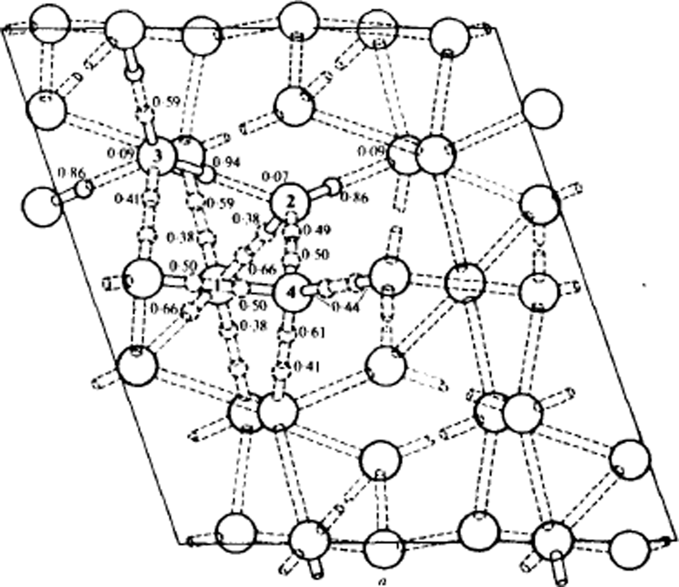
Structure of ice V at 110 K, viewed along the monoclinic b-axis. Oxygen atoms are shown as large circles. Lengths are in Å. Some of the deuteron positions are indicated by small circles, accompanied by the corresponding probability factor. The nearly full deuterons are shown solid, the approximately half deuterons are dashed, and the nearly absent deuterons are not drawn. The dotted rods are the hydrogen bonds. The details of bond lengths and angles are omitted. (After Reference Hamilton, Hamilton, Kamb, LaPlaca, Prakash, Riehl, Riehl, Bullemer and EngelhardtHamilton and others, 1969.)

Fig. 11.

The structure of ice VI. In column A the hydrogen-bond chains running vertically through the structure are shown. The lower one is identical to the upper but turned through a right-angle. The three-dimensional structures formed from these chains are shown in B, while in C the two structures shown in B are combined to form the complete structure of ice VI in which the two components interpenetrate. Protons are not shown. (After Reference KambKamb, 1965.)

Fig. 12.

The structure of ice VII. This is body-centred cubic but hydrogen bonds are limited to four per oxygen molecule and form two interpenetrating ice Ic structures. The protons are shown disordered. With the protons ordered, the structure would be that of ice VIII. (After Reference Kamb and DavisKamb and Davis. 1964.)

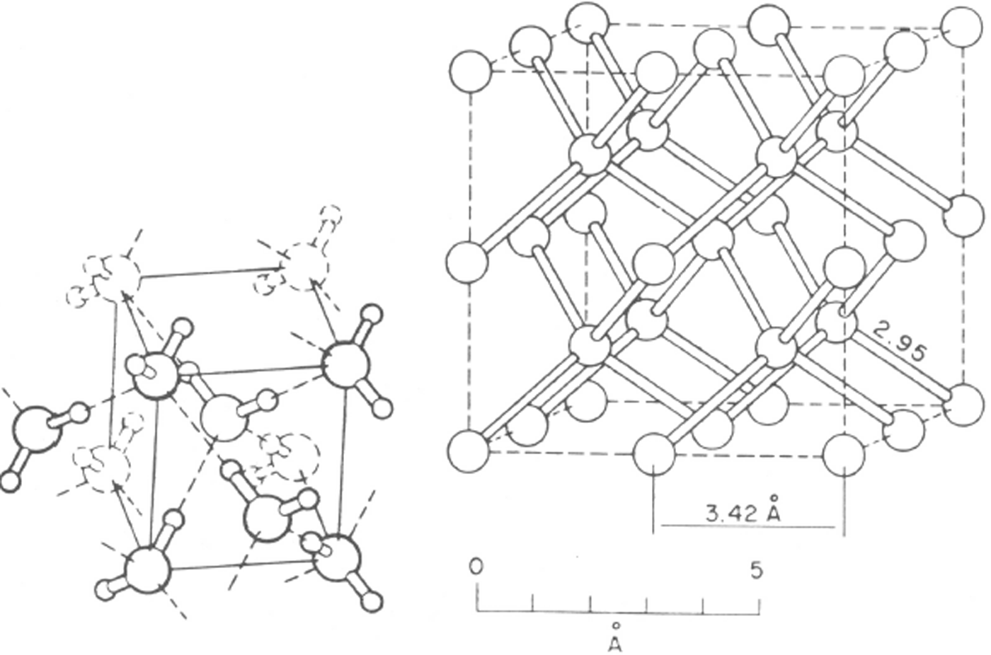
The cubic arrangement that appears in ice VII is also sometimes observed as a simple structure, (not interpenetrating) at low pressures. When ice is formed from the vapour at around –120 °C or when high-pressure ices transform as they are warmed up, then this ice, known as ice Ic, is formed. This was first observed by Reference KönigKönig (1943). At still lower temperatures ice is deposited in vitreous or amorphous form. This also transforms to ice Ic when heated. It seems doubtful however whether ice Ic is ever the stable form of ice.

Knowing the arrangement of water molecules in ice is one aspect of an understanding of ice crystals, knowledge of the way in which ice crystals develop in Nature is another to which very much effort has been devoted over the half century under review. In particular, the development of ice crystals from water vapour has received much attention because of its great importance to meteorologists. Snow crystals have long been seen and admired, but 50 years ago the reasons for the great variety of snow-crystal forms were largely unknown. Nakaya's pioneering experiments on the growth of ice crystals in a controlled environment (artificial snow crystals) were first reported in 1938 and the book summarizing his work was published in 1954 (Reference NakayaNakaya, 1954). These experiments established that both temperature and super-saturation were important in determining the growth habit of snow crystals which varied from needles elongated in the [0001] direction to scrolls, cups, columns, plates, and planar dendrites (Fig. 13). Furthermore, the variation was not monotonic; it appeared to reverse so that, for example, plates appear at both higher and lower temperatures than those appropriate for dendrites. The reason for this rapid change in behaviour has been the subject of many theories throughout the remaining decades.

Fig. 13.

The various shapes of ice crystals which form under different conditions of temperature and supersaturation. The solid line W marks the limit of supersaturation with respect to liquid water (supercooled). (After Reference NakayaNakaya, 1954.)

In addition to the information given by snow-crystal shapes concerning the conditions in the clouds when they were formed, a number of other aspects of ice physics have been much debated by cloud .physicists, in particular the possible role of the electrical properties of ice in the generation of thunderstorm electricity. Ice physics has also become of interest to astronomers, both because of the existence of ice particles as constituents of dust in space and because of the existence of larger ice masses in comets, on planets, and on satellites of planets, some of which may be largely composed of ice. Thus, the interest in the results of ice-physics research has expanded from the original areas of geology and geography to meteorology and astronomy and, increasingly, to engineering problems as increasing developments occur in cold regions.