INTRODUCTION
The question whether “expectations matter” and may cause excess price volatility, above and beyond volatility driven by news about underlying economic fundamentals, has been a matter of heavy debate among economists for many decades already. In a pioneering paper, Shiller (1981), for example, argued that stock prices are excessively volatile. The present paper may be viewed as an experimental testing of expectation formation and learning in a dynamic market setting. We employ the simplest of all dynamic economic market models, the classical cobweb or “hog cycle” model, to investigate whether agents learn the unique steady state rational expectations equilibrium (REE) or whether excess price volatility is a persistent phenomenon.
In modeling price movements in real markets, the expectations hypothesis is a key assumption. Any dynamic economic model has a self-referential or expectations feedback structure, where expectations about future variables affect realizations of actual variables and new realizations in turn lead to new expectations. In modeling dynamic markets this interaction is repeated ad infinitum, and the underlying expectations hypothesis is thus crucial in determining dynamic market equilibrium. Since the pioneering work of Muth (1961) and Lucas (1972), the rational expectations hypothesis (REH) has become (and currently still is) the dominant paradigm in expectation formation in economics and finance. According to the REH, agents use all available information and their subjective expectation equals the mathematical expectation conditional upon this information. In implementing the REH in economic modeling, it is usually assumed that agents have perfect knowledge about market equilibrium equations. The agents in the model use these equations to compute their optimal predictions for future variables. In a rational expectations equilibrium, forecasts coincide (on average) with realizations.
Until the sixties, before the rational expectations (RE) revolution, it was common practice to use simple habitual rule-of-thumb predictors for agents' expectations in dynamic market models. The best-known textbook example is probably the cobweb market equilibrium model or “hog cycle” model with a one-period production lag. Ezekiel (1938) investigated the price dynamics in the cobweb model under naive expectations, where the expected price for tomorrow equals today's price. Nerlove (1958) studied price fluctuations under adaptive expectations, where the expected price is adapted by a constant factor in the direction of the latest observed market price. Under naive or adaptive price expectations, price fluctuations in the (linear) cobweb model are characterized by up and down oscillations around the market equilibrium steady state, either converging or diverging from the steady state price. The rational expectations argument against these mechanical forecasting rules is well known. Agents make systematic forecasting errors along the “hog cycles,” and rational agents would learn from these forecasting errors and revise expectations accordingly. In the cobweb model, the only forecast without systematic errors is the prediction that the price will be at its steady state value where demand and supply intersect. This rational expectations equilibrium is unique and can be derived easily when demand and supply curves are known to the agents.
There seems to be general agreement among economists that the REH assumes too much knowledge on the part of the agents. In particular, the assumption that agents have perfect knowledge of underlying market equilibrium equations is at odds with practice in real markets. In the last decade, much theoretical work has been done on bounded rationality, in an attempt to back off from rational expectations. Instead, in the bounded rationality framework, agents are assumed to form expectations based upon time series observations. Recent surveys on bounded rationality in expectation formation include Sargent (1993, 1999), Evans and Honkapohja (1999, 2001), and Marimon (1997). Boundedly rational agents have some simple model of the world, the perceived law of motion, and try to learn or optimize the parameters of their perceived law of motion, e.g., by an econometric technique such as ordinary least squares as additional observations become available. An important question in the bounded rationality work is whether or not adaptive learning schemes converge to a RE steady state. If convergence occurs, REE will be an accurate description of the realized market equilibrium outcome, at least in the long run, and this REE outcome can be attained without any knowledge of market equilibrium equations.
For the cobweb model, indeed, a number of papers have argued that simple learning rules based upon time series observations enforce convergence to the unique RE steady state. For example, Bray and Savin (1986) show that if agents employ ordinary least squares learning, prices converge to the REE steady state. Arifovic (1994) shows that convergence to the RE equilibrium occurs when agents use genetic algorithm learning. Finally, Hommes and Sorger (1998) have recently shown that, if agents learn the sample mean and the first-order sample autocorrelation from observed past prices and use these in their linear forecasting rule, convergence to the RE steady state occurs. These theoretical papers suggest that, in the cobweb model, learning of simple forecasting rules may stabilize price fluctuations and enforce convergence to the RE steady state, even when market equilibrium equations are unknown. In contrast, however, Chiarella (1988) and Hommes (1994) show that the cobweb model with adaptive expectations need not converge to the RE steady state, but periodic or even chaotic price fluctuations around an unstable steady state can arise. Brock and Hommes (1997) study the cobweb model with heterogeneous expectations and show that under evolutionary learning prices need not converge to the RE steady state. See also Grandmont (1998) and Grandmont and Laroque (1991) for a general discussion of how learning may lead to instability, and Guesnerie (1992, 2002) for a discussion of eductive learning and coordination on rational expectations equilibria. The main conclusion from this theoretical work is that different theories of expectation formation and learning yield contradictory results concerning the stability or instability of the (unique) RE steady state equilibrium in the cobweb framework.
Unfortunately, it is hard to test the expectations hypothesis empirically and to infer the way people form expectations from economic or financial data. Survey data research, as for example by Frankel and Froot (1987) on inflation expectations and by Shiller (1989, 2000) on stock market expectations, yields useful insights on expectation formation but also has its limitations, for example, because of changing underlying economic fundamentals. Controlled laboratory experiments seem to be well suited to investigate which expectation formation hypothesis is most accurate in describing human forecasting behavior and observed aggregate market outcomes in particular situations. As noted, e.g., by Sunder (1995), it is remarkable that, despite an explosion of interest in experimental economics, relatively few contributions have focused on expectation formation and learning in dynamic experimental markets with expectations feedback. Some exceptions are the well-known “bubble experiments” of Smith et al. (1988) in an experimental asset market, the experimental work by Marimon et al. (1993) on the role of price expectations in an inflationary overlapping-generations economy, and the experiments by Marimon and Sunder (1993) on hyperinflation. These studies cannot be viewed, however, as pure experimental testing of the expectations hypothesis, everything else being constant, because in all these cases dynamic market equilibrium is affected not only by expectations feedback but also by other types of human behavior, such as trading behavior. Two other related papers, by Hey (1994) and Kelley and Friedman (2002), focus exclusively on expectation formation on time series generated by stationary stochastic processes. Hey (1994) studies forecasting of a first-order autoregressive process and finds that “subjects are trying to behave rationally, but frequently in a way that appears adaptively.” Kelley and Friedman (2002) consider learning in orange juice futures price forecasting experiments, where prices are driven by a linear stochastic process with two exogenous variables (weather and competing supply). They find that learning is slow but quite consistent, in the sense that estimated coefficients slowly converge to the true values. In these papers, the stochastic process is exogenous, however, so that there is no expectations feedback, as in dynamic market equilibrium models. The key difference with our experiments is the self-referential structure in our setting.
The present paper may be viewed as experimental testing of the expectations hypothesis in what is perhaps the simplest of all dynamic models, the cobweb model. A convenient feature of the cobweb model is that it has a unique REE. Market equilibrium equations are controlled and fixed during the experiment (although they are subject to small demand shocks). Subjects are asked to predict prices and their earnings are inversely related to their quadratic forecasting errors. Price realizations only depend upon subjects' price expectations. In all treatments the experimental environment is stationary and the RE steady state is fixed and constant over time. All experiments are conducted in the CREED Experimental Laboratory of the University of Amsterdam.
There have been a number of earlier “cobweb experiments” related to our work. Holt and Villamil (1986) and Hommes et al. (2000) conducted individual cobweb experiments, where price fluctuations are induced by decisions of a single individual. Carlson (1967) conducted hand-run experiments with subjects as cobweb suppliers. Wellford (1989) conducted several computerized cobweb experiments, where market prices were determined by subjects' quantity decisions. A distinguishing feature of our approach is that market prices are completely determined by forecasts made by a group of individuals, everyting else being constant (only subject to small noise).
Using aggregate realized market prices from our experimental cobweb economy, three important questions can be addressed:
- Are subjects in the experiments “on average” able to learn the unique RE steady state price, or can realized market prices be significantly upward or downward biased?
- Is there evidence of excess price volatility, that is, is the price volatility (as measured by the variance) in the experiments significantly higher than the price volatility under RE?
- If prices do not converge to RE, is there still forecastable structure in realized market prices that could be exploited by “smart” agents?
The paper is organized as follows. Section 2 describes the design of the experiment. Section 3 briefly recalls some benchmark expectation and learning models in the cobweb framework. Section 4 presents the main experimental results, including statistics such as sample mean, sample variance, and sample autocorrelations. Concluding remarks are given in Section 5.
EXPERIMENTAL DESIGN
The well-known cobweb or “hog cycle” model describes price fluctuations in an independent market for a perishable consumption good, such as corn or hogs, that takes one unit of time to produce. Producers thus have to forecast the market price one period ahead. In our cobweb experiments, subjects have to predict the next period's price of a certain unspecified good. The subjects have limited information about this market. Subjects are told that they are advisors to producers of an unspecified good and that the price is determined by market clearing, that is, equality of demand and supply. Subjects are also informed that there is some uncertainty with respect to the demand and/or supply of the good due to market uncertainties, for example, a possibly bad harvest because of extreme weather conditions. Subjects do not know market equilibrium equations, nor are they informed about the distributions of any exogenous shocks to demand and/or supply. Based upon this limited information, we ask the subjects to predict next periods market price for 50 consecutive periods. The predicted price always has to be between 0 and 10 and the realized price is also always between 0 and 10.
The subjects are also informed that their earnings are inversely related to their prediction error: the better their forecast, the higher their earnings. They can earn a maximum of 1300 points per period. The payment in each period is based upon the quadratic payoff function

where
is subject i's prediction of the market price in period t, 1≤ t≤50, and pt is the realized market price in that period. The expected value of this function is maximized by
. Negative payoffs are not possible; earnings are 0 if
. At the end of the experiment the points are exchanged for Dutch guilders at a rate of 1300 points = 1 guilder (≈0.45 Euro).
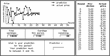
After every period, the subjects are informed about the realized price in the experiment. Also, time series of the subjects' own past predictions and a time series of the past realized prices are shown on the screen, as illustrated in Figure 1.

Typical computer screen of a subject during the experiment. Time series of predictions and realized values were plotted in different colors on the computer screen.
At the beginning of each session, the subjects are asked to read the instructions carefully. Two control questions are put into the instructions to make sure the subjects understand the experiment and the calculation of their earnings. Each session lasts for 50 periods. In each period, the aggregate realized market price depends upon the individual expectations of 6 participants. A small random shock is added to the market equilibrium equation in each period. The composition of the groups remains the same during the entire experiment. Subjects are not informed about the identity of other group members, the size of the group, or the market equilibrium equation. Participants are not informed that the realized price depends upon their forecast of the price and/or upon other forecasts and they are not allowed to communicate. In total there were 108 subjects participating, divided over three different treatments, a stable, an unstable, and a strongly unstable treatment, as discussed below. Each of the three treatments had 36 participants. Each market of 50 periods consists of a fixed group of 6 subjects; for each treatment six markets were run. Subjects (mostly undergraduates in economics, chemistry, and psychology) were recruited by means of announcements on information boards in university buildings. Subjects earned on average FL.26.—(≈12 Euro) in approximately 75 minutes.
Subjects in the experiments thus have very little information about the price-generating process. The information in the experiment is similar to the information assumption underlying much of the theoretical bounded rationality literature, namely that individuals form expectations based upon time series observations.
The realized market price pt in the experiment is determined by the cobweb market equilibrium equation in which demand equals total supply; that is,
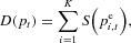
where D(pt) is the demand for the good at price pt, K is the size of the group, S(·) denotes the supply curve, and
is the prediction of the price in period t, made at date t−1 by subject i. In our experiment the number of subjects in one market is fixed at K=6. Solving (2) for the market equilibrium price yields
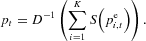
In the experiment the demand curve is fixed and simply linear,

where ηt is a normally distributed random series representing a small demand shock in period t. In all treatments, the parameters have been fixed to a=13.8 and b=1.5. For the supply curve, we use the nonlinear specification

Supply is nonlinear, but increasing in producers' expected price. It should be stressed that because supply is increasing, it is consistent with producers' profit maximization with a convex cost function. The parameter λ tunes the nonlinearity of the supply curve and the stability of the underlying cobweb model. Each of the three treatments corresponds to a different value of the parameter λ. A convenient feature of a nonlinear supply curve is that, under naive or adaptive expectations, prices may diverge from the unstable steady state, but remain bounded and converge to a (unique) stable 2-cycle, as will be discussed below.
Given the (unknown) demand curve (4), the (unknown) supply curve (5), and the individual forecasts of the market price by all participants, the realized market equilibrium price is determined by
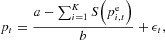
where εt=ηt/b is a (small) noise term proportional to the demand shock ηt. The shocks εt may thus be interpreted as intrinsic uncertainty about economic fundamentals. The shocks εt are normally distributed with variance
; the 50 realizations εt of the random series were the same for each market.
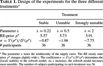
We conducted three different treatments, a stable, an unstable, and a strongly unstable treatment, depending upon the value of the parameter λ tuning the nonlinearity of the supply curve, as summarized in Table 1. Each of the three treatments represents a stationary experimental environment with a fixed and constant RE steady state p*. Learning this constant RE steady state over 50 time periods is made more difficult by the (small) noise terms. Notice also that due to the different values of λ, each treatment has a different RE steady state price p*.

The parameter λ affects the stability of the cobweb model. According to the classical cobweb theorem [e.g., Ezekiel (1938)], under naive expectations the steady state p* is (locally) stable if the ratio σ= S′(p*)/D′(p*) of marginal supply to marginal demand at the steady state is between −1 and 1. For our choice of the demand and supply curves the stability condition becomes
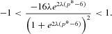
The experimental designs for the three different treatments are summarized in Table 1.
BENCHMARK MODELS OF EXPECTATIONS AND LEARNING
This section briefly summarizes aggregate price fluctuations in the cobweb model under some benchmark models of expectations and learning, including rational expectations, naive expectations, adaptive expectations, and various adaptive learning schemes. In the simulations, demand and supply curves are the same as in the strongly unstable treatment of our cobweb experiments. In Section 4 we will compare our experimental results with the benchmark cases to test which expectations hypothesis fits our experiments best.
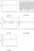
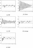
Figure 2 shows realized market prices for the benchmarks of rational expectations (RE), naive expectations (Naive), adaptive expectations (w=0.2), “learning by average,” and sample autocorrelation (SAC) learning, as discussed below. Figure 3 shows the autocorrelations of realized market prices for each of these benchmark cases.

Time series of realized prices for some benchmark cases in the strongly unstable treatment: (a) rational expectations, (b) naive expectations, (c) adaptive expectations (w=0.2), (d) learning by sample average, and (e) SAC-learning.

Autocorrelation plots (with Bartlett 5% significance bands) for the benchmark cases of RE, Naive, AE, learning by average, and SAC-learning in the strongly unstable treatment, over the full sample of 50 periods.
Recall that under RE, producers forecast the price to be equal to the steady state at which demand and supply curves intersect; that is,
. Given that all producers use the RE forecast, realized market prices in (6) are given by

Hence, under RE, realized market prices fluctuate randomly around the RE price p* with small amplitude determined by the variance of the noise term (
), as illustrated in Figure 2a. The autocorrelation plot under RE in Figure 3a shows that price fluctuations are indeed uncorrelated and do not exhibit unexploited (linear) predictable structure.
Naive expectations means that all producers use the latest observed price as their forecast; that is,
. Figure 2b shows realized market prices under naive expectations. This is the familiar “hog cycle,” with prices fluctuating up and down with large amplitude over the entire admissable interval [0, 10]. Figure 3b shows the corresponding autocorrelation plot, exhibiting the regular (−, +, −, +, …) autocorrelation pattern that is typical for regular up and down cobweb “hog-cycles,” with the first 13 lags being strongly significant. Not only do naive producers make large forecasting errors, but these errors are also systematic, because when their forecast
is low (high), the realized market price pt is high (low).
Adaptive expectations (AE) means that all producers use the forecast

that is, producers adapt their forecast in the direction of the latest observed market price with a constant fraction w. Adaptive expectations is therefore sometimes also called constant gain error learning. Notice that w=1 corresponds to naive expectations. Figure 2c shows realized market prices under adaptive expectations for a small adaptive coefficient, w=0.2. The amplitude of the price fluctuations is much smaller than under naive expectations, but clearly larger than under RE. Due to the noise term εt, the price pattern is somewhat irregular, but on the other hand, e.g., between periods 25 and 40, prices still exhibit fairly regular up-and-down oscillations. Figure 3c shows the corresponding autocorrelation plot of realized market prices under AE. The autocorrelations are not as strong as under naive expectations, but still exhibit the regular (−, +, −, +, …) pattern, with the first seven lags being significant. As for naive producers, adaptive expectations producers are thus irrational in the sense that observable forecastable structure in market prices is left unexploited.
Another simple forecasting strategy is by the sample mean, that is,
, where

is the sample mean of all previously observed prices. We will refer to this simple rule as learning by average. This forecasting rule is equivalent to running an ordinary least squares (OLS) regression of prices on a constant, as studied in the cobweb context by Bray and Savin (1986). Figure 2d shows realized market prices under learning by average. The amplitude of the price oscillations quickly decreases, and prices seem to converge to RE, with random fluctuations around the constant RE steady state price after 10 time periods. The corresponding autocorrelation plot is shown in Figure 3d with hardly any significant autocorrelations.
A final learning rule, introduced recently by Hommes and Sorger (1998), is sample autocorrelation learning (SAC learning), where producers use a linear forecasting rule,

and update the parameters αt by the sample average and βt by the first-order autocorrelation coefficient. Figure 2e shows realized market prices under SAC-learning. The amplitude of the price oscillations quickly decreases, and prices seem to converge to RE, with random fluctuations around the constant RE steady state price after 10 time periods. SAC learning has significant negative autocorrelations at lags 2 and 3, but this is mainly caused by the initial large amplitude price fluctuations; when restricted to the last 40 observations, that is, after SAC learning converges to the RE steady state, these significant autocorrelations disappear.
Figures 2 and 3 show that for our strongly unstable treatment of the cobweb experiments, different expectations schemes and learning models lead to different types of price fluctuations. Mechanical forecasting rules such as naive or adaptive expectations lead to large-amplitude price fluctuations with linear forecastable structure in market prices. It is important to note that, even in the strongly unstable case, simple learning schemes, such as learning by average, OLS learning, and SAC learning, enforce convergence to RE. Hence, even for a strongly unstable cobweb market producers may learn the RE price from time series observations, without any information about underlying market equilibrium equations. The goal of our experiments is to investigate whether this theoretical observation is valid in our cobweb laboratory experiments.
EXPERIMENTAL RESULTS
This section reports the results of the experiment. In Section 4.1 the earnings of the participants are discussed, whereas Section 4.2 focuses on the first two moments of realized market prices, namely, the sample mean and the sample variance. We compare these sample means and sample variances to the theoretical benchmark cases of Section 3, and in particular we investigate whether market prices are biased (i.e., whether the sample mean deviates from the RE steady state) and excessively volatile (i.e., whether the sample variance of realized market prices is significantly larger than the RE variance). Finally, the predictability of realized market prices, as measured by sample autocorrelation patterns, is investigated.
Earnings
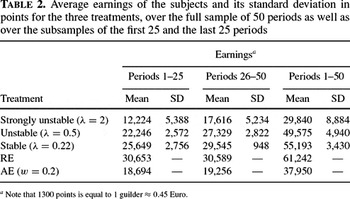
Table 2 summarizes the average earnings over the subjects and their standard deviation for the stable, unstable, and strongly unstable treatments, as well as for the RE and AE benchmarks. The AE earnings reported in the table were computed with the supply curve as in the strongly unstable treatment and with adaptive coefficient w=0.2. Note that the RE earnings reported in the table are equal for all treatments, because under RE the forecasting errors are equal to the realizations of the shocks εt in (7), which were identical for all treatments. An immediate observation from the table is that the average earnings in the stable treatment are higher than the average earnings in the unstable and the strongly unstable treatments. For all treatments the average earnings in the last 25 periods are higher than in the first 25 periods. Although the total average earnings of the stable and the unstable treatments do not differ a lot (only 6,000 points), the difference between the unstable and the strongly unstable is much bigger (almost 20,000 points). More importantly, the average earnings in the stable treatment are close to the average earnings in the RE benchmark, especially in the subsample of the last 25 periods. Furthermore, the total average standard deviation in the stable treatment is smallest. In the last 25 periods of the stable treatment, the standard deviation is almost three times smaller than in the first 25 periods. For both the unstable and the strongly unstable treatments this is not the case. To summarize, when the model becomes more stable, the average earnings of the subjects increase, whereas the difference in earnings decreases.

Testing the Rational Expectations Hypothesis
In this section we investigate whether the RE hypothesis is an accurate description of realized aggregate market prices, with or without a learning phase. Stated differently, we investigate whether realized market prices in the experiments converge to the RE steady state. We investigate the validity of RE as a description of aggregate price fluctuations by focusing on three important characteristics, namely whether realized market prices are biased, whether price fluctuations exhibit excess volatility, and whether realized prices are predictable. It seems natural to measure these characteristics by the mean, the variance, and the autocorrelation patterns of realized market prices and compare these to the corresponding RE characteristics. We investigate and compare these characteristics for all treatments.
Price dynamics
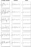
Figure 4 shows the realized prices for all treatments, with the strongly unstable treatment in the left panel, the unstable treatment in the middle panel, and the stable treatment in the right panel. In all markets, prices seem to fluctuate irregularly without any clear pattern. By eye inspection, it is immediately clear that in the strongly unstable treatment, the amplitude of the price fluctuations is much larger than in the unstable and the stable treatments. In the stable treatment (right panel), the amplitude of the price fluctuations is small and seems surprisingly close to the RE benchmark (cf. Figure 2a). In the unstable treatment (middle panel), the amplitude of the price fluctuations is larger and decreases somewhat over time. In the strongly unstable treatment (left panel), the amplitude seems to be much larger than in the RE benchmark, suggesting excess price volatility. Only for group 1 (top left) of the strongly unstable treatment does the amplitude of the price oscillation decrease over 50 time periods. This group thus shows some form of learning and at least a tendency to converge to RE, although the convergence seems to be much slower than, e.g., in the SAC benchmark (cf. Figure 2d).

Time series of realized prices of the six groups in the strongly unstable treatment (left panel), the unstable treatment (middle panel), and the stable treatment (right panel).
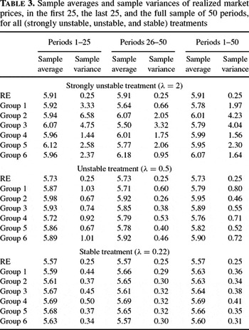
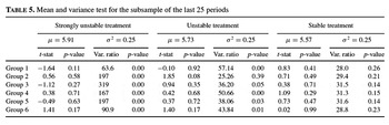
To investigate the validity of the RE hypothesis in our experiment, Table 3 shows the sample mean and sample variance of the realized prices for the stable, the unstable, and the strongly unstable treatment for the full sample of 50 periods, as well as for subsamples of the first 25 and the last 25 periods. For all treatments, the sample average of realized market prices is surprisingly close to the RE benchmarks of 5.91, 5.73, and 5.57, respectively. Over the full sample of 50 periods, in the strongly unstable treatment the sample variance ranges from 1.56 to 4.23, which is much higher than the variance 0.25 of the RE benchmark. In the unstable treatment the sample variance of realized prices ranges from 0.46 to 0.80, which is also larger than the RE benchmark. In the stable treatment, the sample variance of realized prices over the full sample of 50 periods ranges from 0.31 to 0.41, which is only slightly higher than the RE benchmark of 0.25. In the subsample of the last 25 periods, the sample variance in the stable treatment ranges from 0.29 to 0.32, which is remarkably close to the variance under RE. In contrast, for the unstable treatment, and for the strongly unstable treatment, in the subsample of the last 25 periods, the sample variance ranges from 0.26 to 0.60 and from 0.66 to 3.32 respectively, which is much higher than the variance under RE.

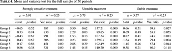
Table 4 shows the results for statistical tests comparing both the sample mean and the sample variance of realized market prices to the theoretical RE-benchmarks. Using the t-statistic, the null hypothesis that the sample mean of realized market prices is equal to the RE steady state price can not be rejected for 17 out of 18 groups in the stable, the unstable, and the strongly unstable treatments. The only exception is group 2 of the unstable treatment, for which the null hypothesis is rejected at the 5% level. Table 4 also shows the results for testing the null hypothesis that the sample variance of realized market prices is equal to the variance under RE over the full sample of 50 periods. For all groups in the unstable and the strongly unstable treatments, the null hypothesis is rejected at the 1% level. For two groups in the stable treatment (groups 2 and 6), we can not reject the null hypothesis at the 5% level. The earlier observation that, over the full sample, the amplitude of price fluctuations is larger than under the RE benchmark is thus statistically significant in all unstable cases and even in four stable cases.

It seems reasonable, however, to allow for some learning phase in the unknown, stationary cobweb environment. Table 5 shows the results for the statistical tests comparing both the sample mean and the sample variance of realized market prices over the subsample of the last 25 periods to the theoretical RE-benchmarks. In all cases, the null hypothesis that the sample mean of realized market prices equals the RE steady state price can not be rejected. In this sense, subjects are thus able to learn the correct price level. For the stable treatment, also, the null hypothesis that the sample variance of realized prices is equal to the variance under RE can not be rejected. For the unstable treatment this null is rejected at the 5% level in five out of six cases, and for the strongly unstable treatment in all cases. This suggests that in the stable treatment participants are on average able to learn the RE steady state price. In the stable treatment, the first two moments of the long-run empirical distribution of realized market prices correspond to the first and second moment of the RE benchmark. In the unstable and the strongly unstable treatments, only the first moment, the mean, corresponds to the RE benchmark, whereas the second moment, the sample variance, is significantly larger than for the RE benchmark. In the unstable and the strongly unstable treatments, although subjects are able to learn the correct price level, even after a learning phase of 25 periods, our cobweb experiments still exhibit statistically significant excess volatility in prices.

Predictability of prices
Finally, we investigate whether there is still forecastable structure in realized market prices that could have been exploited by smart subjects to improve their forecasts. The simplest and perhaps most important form of predictability is linear predictability, as measured by sample autocorrelations.
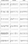
Figure 5 shows the sample autocorrelation plots for the strongly unstable treatment (left panel), the unstable treatment (middle panel), as well as for the stable treatment (right panel). An immediate and important observation from Figure 5 is that realized market prices show no clear autocorrelation pattern, with hardly any significant lags. The only group exhibiting a clear and regular autocorrelation pattern is group 5 of the strongly unstable treatment, which is characterized by the regular (−, +, −, +, …) autocorrelation pattern that was also observed for the AE benchmark. However, in contrast to AE, for group 5 only lags 1, 5, 7, 11, 15, and 16 are significant. In general, significant autocorrelations are rare, and in our cobweb experiments realized market prices exhibit (almost) no linear predictable structure. In terms of (linear) predictability the RE benchmark is thus a good description of our cobweb experiments. Even in the unstable and the strongly unstable case, where we found significant excess price volatility in Section 4.2.1 and market prices kept fluctuating with relatively large amplitude, participants in the experiment are not irrational, in the sense that there is no easily exploitable predictable structure in realized market prices.

Autocorrelation plots over the full subsample of 50 periods (with Bartlett 5% significance bands) for the six groups in the strongly unstable treatment (left panel), the unstable treatment (middle panel), and the six groups in the stable treatment (right panel).
CONCLUDING REMARKS
We have investigated expectation formation and learning in cobweb experiments. The realized market price is determined by aggregation over six individual price forecasts. Market equilibrium equations, as well as distributions of exogenous shocks, are unknown to subjects. Subjects can only rely upon past observations of realized prices in forming expectations. Market equilibrium equations are fixed and thus stationary for 50 time periods, so that each market has a unique and constant RE price. A distinction is made between a stable, an unstable, and a strongly unstable treatment. In the stable treatment under naive expectations, prices will converge to the RE steady state price, whereas in the unstable and the strongly unstable treatments under naive expectations, prices diverge from the RE steady state and converge to a 2-cycle. Simple benchmark models of learning, such as learning by sample average, enforce convergence to the RE steady state price for all three different treatments. An important motivation for our paper is to investigate, in a controlled stationary laboratory environment, which expectations hypothesis yields an accurate description of aggregate realized market prices in a cobweb-type commodity market. In particular, we investigate whether the RE benchmark provides a good description of long-run market price fluctuations.
For all treatments, the null hypothesis that the sample mean of realized market prices is different from the RE steady state price can not be rejected. One thus can say that in a stationary experimental cobweb economy the first moment, the mean, of the empirical distribution of realized market prices corresponds to the RE steady state price. Without any knowledge about market fundamentals, subjects are thus on average able to learn the correct price level.
In the stable treatment the second moment, the sample variance, of realized market prices also is very close to the variance under RE. In the stable treatment, the null hypothesis that the sample variance in the last 25 periods is equal to the sample variance under RE can not be rejected. In contrast, in the unstable and the strongly unstable treatments the null hypothesis that the sample variance of realized market prices is (smaller than or) equal to the sample variance under RE is strongly rejected. For all groups in the strongly unstable treatment and five out of six groups in the unstable treatment, realized market prices exhibit statistically significant excess volatility, that is, higher price volatility than under RE.
For all treatments, predictability of realized market prices was investigated by sample autocorrelations. Typically, (almost) no significant sample autocorrelations are found, implying that there is little predictable structure left in realized market prices that could have been easily exploited by “smart” participants. Although in the unstable treatments prices keep fluctuating with large amplitude, these fluctuations are irregular and fairly unpredictable.
Which expectations hypothesis is a good description of aggregate realized market price fluctuations in a cobweb economy? The answer to this question depends on the stability of the model. If the market is stable (under naive expectations), RE is a fairly good description, at least after a short learning phase. Hence, even when agents do not know market equilibrium equations, the RE equilibrium concept may be a useful description of aggregate market outcome. If the market is unstable, however, RE is not a good description, since we find significant and persistent excess price volatility. It is remarkable that the validity of RE exactly coincides with the stability of the simple naive expectations rule. Adaptive expectations are not a good description of the experiments, because they typically lead to fairly regular up-and-down price oscillations with regular autocorrelation patterns in realized market prices. Neither are adaptive learning schemes such as learning by sample average or ordinary least squares (OLS) learning good descriptions of our experimental outcomes, because these schemes always converge quickly to RE. The experimental outcome for an unstable cobweb economy may be described as a boundedly rational heterogeneous expectations equilibrium, where subjects are on average able to learn the correct price level, but diversity of beliefs leads to excess price volatility. More work on individual prediction strategies is needed to classify individual forecasting strategies.
Finally, we would like to discuss to which market institutions our results may apply. In a cobweb-type commodity market, aggregate equilibrium prices are driven by producers' individual price expectations. A key feature of the cobweb expectations feedback structure is that it is self-reversing in the following sense. A high (low) price expectation of the producers leads to high (low) production which, by market equilibrium of demand and supply, leads to a low (high) realized market price. The cobweb commodity market is thus a producer-driven negative expectations feedback system. Our experiments show that in a stationary environment with a negative expectations feedback structure, without any knowledge about market equilibrium equations, subjects are able to learn the correct price level. Apparently, persistent under- or overvaluation does not arise in a commodity market with a negative expectations feedback structure. This does not imply that prices will converge to a steady state equilibrium price in such a market. The amplitude of realized market price fluctuations depends heavily on the sensitivity of the realized market equilibrium price to individual expectations. Our cobweb experiments provide an example of how in a market where the realized market price is very sensitive to expectations, excess volatility, with large-amplitude fluctuations around the correct price level, may arise.
There is another, different expectations feedback structure that seems important and particularly relevant in speculative asset markets. In a speculative asset market, expectations are typically demand-driven and are often self-fulfilling in the following sense. The aggregate demand for a risky asset depends upon traders' individual expectations of future prices of the asset. High (low) price expectations of individual agents lead to a high (low) aggregate demand for the asset which, by market equilibrium of demand and supply, leads to a high (low) realized market price. A speculative asset market is thus a demand-driven positive expectations feedback system. In a recent Ph.D. thesis van de Velden (2001) shows that in an experimental speculative asset market it is indeed much harder for subjects to learn the correct price level and persistent over- or undervaluation and price bubbles seem more likely than in the producer-driven commodity market considered in this paper. In another recent paper, Hommes et al. (2005) present asset-pricing laboratory experiments where individuals coordinate their expectations on simple trend-following rules, leading to (temporary) bubbles and asset price fluctuations around a constant bechhmark fundamental price. We conclude that the market institution and in particular the nature of the expectations feedback structure, whether it is producer- or demand-driven and whether the feedback is positive or negative, seems to be a key element for the outcome of a learning process of market equilbrium prices. More experimental work is needed to investigate this key problem in dynamic market phenomena in more detail.
We would like to thank Vernon Smith and Shyam Sunder for stimulating discussions. This research has been supported by the Netherlands Organization for Scientific Research (NWO) under a NWO-MaG Pionier grant. Earlier versions of this paper were presented at the Annual Meeting of the Economic Science Association, Lake Tahoe, May 27–30, 1999, the CeNDEF workshop on Economic Dynamics, Amsterdam, January 13–15, 2000 and the 7th Viennese Workshop on Optimal Control, Dynamic Games and Nonlinear Dynamics: Theory and Applications in Economics and OR/MS, Vienna, May 24–26, 2000 and the conference on “Belief Formation and Fluctuations in Economic and Financial Markets,” Heidelberg, December 12–13, 2002 sponsored by the Volkswagenstiftung. Stimulating discussions with participants are gratefully acknowledged.