1 Introduction
A number of different numerical, experimental or theoretical studies regarding flows past multi-scale turbulence generators, fractal grids (FGs) in particular, have been reported to the scientific community over the past decade. Pioneering works, i.e. Hurst & Vassilicos (Reference Hurst and Vassilicos2007), Seoud & Vassilicos (Reference Seoud and Vassilicos2007), Mazellier & Vassilicos (Reference Mazellier and Vassilicos2010), showed that the properties of the flow fields behind fractal grids deviate from those observed past regular grids (RGs) in several ways, e.g. a different scaling of turbulent kinetic energy or the constancy of the ratio between an integral length scale and a Taylor length scale was observed. Further studies subsequently investigated a wide range of aspects of these flows, amongst which their stirring and mixing capabilities are of particular interest for the present work. Note that these two terms are not equivalent; mixing should be associated with the decay of a scalar concentration field’s fluctuations whereas stirring should be associated with a spatial redistribution of the patches of scalar.
An initial study on fractal turbulence generators was performed by Coffey et al. (Reference Coffey, Hunt, Seoud and Vassilicos2007). The researchers showed that this kind of geometry can be utilised to improve static in-line mixer performance substantially. Further, Suzuki et al. (Reference Suzuki, Nagata, Sakai and Ukai2010) experimentally compared the spreading rates of scalar mixing layers in turbulent flows past FGs and RGs (Schmidt number
 $Sc=2100$
). The authors showed that the width of the layer, measured with either the mean concentration or the concentration’s variance, is greater for FGs at a comparable normalised downstream location (note that this was normalised with an effective mesh size, being a function of the grid’s geometry). Laizet & Vassilicos (Reference Laizet and Vassilicos2012) provided numerical evidence that the transverse turbulent scalar flux is highly enhanced in the flow past a FG, by up to an order of magnitude. This was reported in the context of the flow with a constant mean scalar gradient (
 $Sc=0.1$
). The authors suggested a plausible physical scenario that could explain the observed enhancement, which they referred to as the space-scale unfolding (SSU) mechanism. The essence of the postulated SSU mechanism is that by varying the sizes of particular elements of a turbulence generator, intersections of their corresponding wakes are shifted to different downstream positions (i.e. spatial unfolding occurs). A fluid element that is initially trapped in one of the smaller wakes can be easily entrained into a bigger wake once the two intersect. By repeating this scenario every time a bigger wake is encountered (which is possible due to the unfolding), the element’s transverse displacement can increase considerably. Results reported in the cited work were further confirmed by Laizet & Vassilicos (Reference Laizet and Vassilicos2015) who performed some numerical simulations in an almost identical configuration (
 $Sc=0.1{-}0.2$
). Additionally, the authors presented results of particle tracking in turbulent flows generated by FGs and RGs (note that these were planar simulations). The variance of the particles’ transverse displacement was considerably higher (by a factor of
 $5$
at least) for the multi-scale configuration. Importantly from the perspective of the subsequent discussion, even in the case where the thickness of the RG’s bars exceeded the thickness of the widest bar of the FG the latter’s stirring performance was superior to the RG.
Contrastingly, Nedić & Tavoularis (Reference Nedić and Tavoularis2016) showed experimentally (
 $Sc=0.7$
) that the width of a plume released into a turbulent flow from a line source depends rather on the thickness of the thickest bar of the turbulence generating grid than on the grid’s topology. This observation was consistent irrespective of the relative positions of the grid and the source. The authors noticed that the thickness of the thickest bar was not preserved between FGs and RGs in most of the previous studies and thus an apparent superiority of FGs could have been observed. The importance of the thickest bar is also stressed by Zhou et al. (Reference Zhou, Nagata, Sakai, Suzuki, Ito, Terashima and Hayase2014) who compared the performance of FGs and a corresponding single-square grid (SSG; the thickness of its bars was set equal to the thickest bar of the FG) in their numerical study. The results of their numerical experiment suggest that the thickest bars are responsible for the majority of the FG’s characteristics, especially in the far field. The finer-scale geometrical details can be considered as a source of additional background turbulence that affects the development of the largest bar’s wake and enhances turbulent mixing in the near-field region. Melina et al. (Reference Melina, Bruce, Hewitt and Vassilicos2017) also compared flows past FGs and SSGs and reported complementary experimental results. The flow field properties past FGs and SSGs approach each other as the downstream coordinate grows. Furthermore, heat transfer performance was nearly the same for the SSG and FG (whilst noticeably different for a RG).
It follows from this brief literature review that there is a controversy regarding whether the stirring efficiency of a turbulent flow downstream of a grid is dictated by the largest forced length scale or the grid’s specific topology. The present experimental work aims to advance this debate by challenging the SSU mechanism – the concept which was introduced by Laizet & Vassilicos (Reference Laizet and Vassilicos2012) and Laizet & Vassilicos (Reference Laizet and Vassilicos2015) as a plausible explanation for their observations. Note that, although clear evidence of different characteristics of stirring behind RGs compared to FGs has been provided by these authors (i.e. the enhanced turbulent scalar flux), the SSU mechanism has not been verified up until now. This verification is performed by arranging an experiment that would mimic the set-up described in the SSU scenario (i.e. a fluid parcel, located in a relatively small-scale wake, encounters an intersection with progressively larger wakes) and attempting a visualisation of the process. Note that the description of the SSU mechanism relies only on the multi-scale nature of the turbulence generation. Therefore, a relatively simple multi-scale geometry can be utilised in this study, i.e. an array of bars of non-uniform thickness, as opposed to complex FGs. This should help to avoid interference with potential secondary effects induced by a complex design of the turbulence generator, which could complicate interpretation of the observations. A flow past a single-scale array is considered for comparison in some cases (note that the SSU description contrasts flows past single- and multi-scale geometries). The scalar tracer is released into the flow behind the array’s thinnest bar (following the scenario given by Laizet & Vassilicos (Reference Laizet and Vassilicos2012)) and further tracked by means of qualitative and quantitative planar laser induced fluorescence (PLIF measurements). Some of these results are complemented by simultaneous velocity field measurements, taken by means of particle image velocimetry (PIV). The experiment is focused on the near-wake area (intersections of particular wakes occur there), which is dominated by relatively energetic sheddings from different bars. Therefore, a triple decomposition is utilised (see Hussain & Reynolds Reference Hussain and Reynolds1970) in the analysis of the results to distinguish between the importance of particular coherent fluctuations and the stochastic fluctuation contribution.
The velocity fields in the flows past the same arrays have been investigated recently by Baj & Buxton (Reference Baj and Buxton2017). The main reported finding is that multi-scale generated turbulence is rich in a number of distinctive coherent fluctuations on top of the quasi-stochastic turbulent fluctuations. Apart from the primary coherent fluctuations associated with the shedding of particular bars, prominent secondary coherent motions are observed to arise as a consequence of triadic interactions between the primary shedding modes. Interestingly, the appearance of the secondary modes is observed in the vicinity of the wake intersection points, which is reminiscent of the SSU concept. By making use of the multi-scale triple decomposition described in Baj, Bruce & Buxton (Reference Baj, Bruce and Buxton2015) we will tackle the second objective of this manuscript, namely to identify the flow physics that underpin the SSU mechanism. As postulated, the SSU mechanism is related to the varying integral length scales present in multi-scale generated turbulence. However, in light of the findings of Baj & Buxton (Reference Baj and Buxton2017) the significance of both the primary and secondary coherent velocity fluctuations is of particular interest for the SSU mechanism.
In this manuscript we will try to verify the SSU concept as a physical mechanism and attempt to reconcile the opposing positions within the literature relating to the efficacy of multi-scale stirrers, namely that the size of the largest bar is the only significant factor versus the fact that the multi-scale geometry modifies the topology of the flow in a favourable sense. We have devised a specific experimental configuration to directly mimic the original postulation of the SSU mechanism from Laizet & Vassilicos (Reference Laizet and Vassilicos2012). We seed scalar into the wake of the smallest obstacle of a multi-scale array and compare the (time-dependent) dispersion of this scalar to that in a single-scale array of similar blockage. Verification of the SSU mechanism will thus depend on observing ‘bursts’ of scalar being exchanged at, or close to, the wake intersection points of the various intersecting wakes downstream of the multi-scale array. However, as shown in Baj & Buxton (Reference Baj and Buxton2017), large-scale coherent motions are dominant in the near field of both the single-scale and multi-scale arrays, with the most energetic motion being that corresponding to the shedding of the largest obstacle present. By deploying the multi-scale triple decomposition technique of Baj et al. (Reference Baj, Bruce and Buxton2015) we can track all of the coherent motions present in the flow and hence assess the relative importance of the largest bar versus the combination of different bars, and hence the multi-scale nature of the geometry, in stirring the scalar. Thus it may be possible, to some extent, to reconcile the claims of Laizet & Vassilicos (Reference Laizet and Vassilicos2015) and Nedić & Tavoularis (Reference Nedić and Tavoularis2016).
Let us briefly introduce the outline of the paper. Section 2 reports details of the experimental facility and the experiment’s design. Section 3 presents the details of the PLIF calibration and quantification technique (a relatively complex quantification methodology proposed by Baj, Bruce & Buxton (Reference Baj, Bruce and Buxton2016) is utilised). Section 4 delivers the main results: qualitative PLIF observations and quantitative results regarding concentration and velocity fields. The latter includes some basic statistics as well as the outcomes of the triple decomposition and conditional averaging. The work is concluded in § 5. Some specific issues are also discussed in the appendix.
2 Experimental set-up
The experimental campaign was conducted in the hydrodynamics laboratory of the Department of Aeronautics at Imperial College London. The main set of measurements utilised an open water channel having a square cross-section whose side length was
 $H=600~\text{mm}$
. Additionally, an auxiliary experiment was performed in a small tank of
 $350\times 250\times 400~\text{mm}$
size.
2.1 The main experiments
Flows past a single-scale and a multi-scale array of bars were investigated in the main experiments. All the measurements were taken at the same inlet velocity
 $U_{\infty }=0.2~\text{mm}~\text{s}^{-1}$
, yielding a global Reynolds number
 $Re_{H}=U_{\infty }H/\unicode[STIX]{x1D708}=120\,000$
(
 $\unicode[STIX]{x1D708}$
denotes the kinematic viscosity). The water depth was set to
 $H$
(the arrays were completely immersed in water). The turbulence intensity
 $I_{T}$
, defined in the context of planar two-dimensional (2-D) velocity data as
 $I_{T}=\sqrt{1/2(u_{1}^{\prime 2}+u_{2}^{\prime 2})}/U_{\infty }$
, of the free stream was found in a preliminary test not to exceed
 $1.9\,\%$
in the bulk flow (see the profile in figure 1(b), the transverse coordinate
 $y$
equals
 $0$
at the flume’s centreline and
 $-H/2$
at its floor) and to approach around
 $12\,\%$
in the turbulent boundary layer near the flume’s floor. The boundary layer thickness, i.e. the distance where
 $99\,\%$
of
 $U_{\infty }$
is recovered, reached
 $65~\text{mm}$
(i.e.
 $0.11H$
) at a downstream position where the test section was located (see the mean streamwise velocity
 $\bar{u}$
profile in figure 1
a).
Characterisation of the free stream at the channel’s centreplane: (a) the mean streamwise velocity profile, (b) the turbulence intensity profile.

The investigated arrays (see figure 2
a,b) consisted of particular bars, which were held within an outer frame (see figure 2
c), whose outer dimension matched the channel’s cross-section. In order to minimise the frame’s impact, streamlining elements were attached to the frame’s bars. The blockage was similar for both grids,
 $27.9\,\%$
and
 $26.7\,\%$
for the single and multi-scale array respectively based on the frame’s inner cross-sectional area (the total blockage reaches
 $39.6\,\%$
and
 $38.6\,\%$
when the frame is also taken into account). The multi-scale array was composed of a big bar, located centrally, and medium and small bars distributed symmetrically about the big one. The bar thicknesses
 $t^{i}$
were equal to
 $76.2~\text{mm}$
,
 $25.4~\text{mm}$
and
 $9.6~\text{mm}$
(
 $0.127H$
,
 $0.042H$
,
 $0.016H$
) for the big, the medium and the small bars respectively (they are referred to as bars
 $I$
,
 $II$
and
 $III$
hereafter). The thickness based Reynolds numbers
 $Re_{t}^{i}=U_{\infty }t^{i}/\unicode[STIX]{x1D708}$
fell into an interval 1900–15 000. The streamwise depth of the bars was equal to
 $15~\text{mm}$
. The gaps between the adjacent bars were equal to
 $70.1~\text{mm}$
between the big and the medium bars (
 $0.12H=0.92t^{I}$
) and
 $60.4~\text{mm}$
between the medium and the small bars (
 $0.10H=2.38t^{II}$
). Spacing between the outer bars (i.e. the farthest most from the centreline) and the frame was set to
 $71.0~\text{mm}$
, which translates into a distance from the channel’s floor/water surface of
 $96.4~\text{mm}$
(
 $0.16H$
). Note that this means that the small bar was not submerged in the boundary layer. This specific configuration of the multi-scale array was picked to ensure: (i) the blockage level is comparable to the blockage of FGs considered by Laizet & Vassilicos (Reference Laizet and Vassilicos2015), (ii) a similar thickness ratio between consecutive scales, (iii) the streamwise position of the intersection of the small and medium wakes is closer to the origin than the intersection of the medium and big wakes (following the description of the SSU mechanism proposed by Laizet & Vassilicos (Reference Laizet and Vassilicos2012)). The single-scale array was composed of six equidistant medium bars at a spacing of
 $65.8~\text{mm}$
(
 $0.11H=2.59t^{II}$
). The gap between the outer bars and the channel’s floor/water was set to
 $72.0~\text{mm}$
(
 $0.12H$
). Note that this configuration of the single-scale array yields a similar blockage and wetted perimeter to the multi-scale case (these two parameters being matched by Laizet & Vassilicos (Reference Laizet and Vassilicos2012, Reference Laizet and Vassilicos2015) for comparisons between FGs and RGs).
(a) Multi-scale grid, (b) single-scale grid, (c) the outer frame.

Three separate sets of experiments were performed: (i) qualitative PLIF and two-dimensional two-components (2D-2C) PIV measurements, (ii) a quantitative PLIF measurement and (iii) a simultaneous quantitative PLIF and 2D-2C PIV measurement (referred to respectively as experiments
 $1$
,
 $2$
and
 $3$
hereafter). Sketches of the set-ups are presented in figure 3. Experiments
 $1$
and
 $3$
focused on the mid-plane of the channel whilst in the case of experiment
 $2$
a cross-stream plane (i.e. plane perpendicular to the flow direction) was monitored. In each case the camera and the optics were fixed at the same position (4.5 m downstream of the channel’s entrance), whilst the array was mounted to a traverse allowing adjustments to its relative upstream position. The differences of the initial conditions that arose at different positions of the array were negligible, i.e. the boundary layer thickness varied by less than
 $10\,\%$
along the measured streamwise extent (figure 1 refers to the farthest most position).
Schematic of the experimental set-up: (a) experiments
 $1$
and
 $3$
, (b) experiment
 $2$
.

Experiment
 $1$
consisted of a single measurement station. Two cameras working simultaneously in a side-by-side arrangement were utilised in this case. The stitched field of view (FOV) size was equal to
 $\unicode[STIX]{x1D6E5}_{x}^{FOV}/H\times \unicode[STIX]{x1D6E5}_{y}^{FOV}/H=0.78\times 0.65$
. Its exact location is indicated in figure 4. Experiment
 $2$
consisted of three measurement stations centred on
 $x/H=\{0.21,0.33,0.45\}$
. The cross-stream concentration distribution was monitored within a FOV having size
 $\unicode[STIX]{x1D6E5}_{y}^{FOV}/H\times \unicode[STIX]{x1D6E5}_{z}^{FOV}/H=0.23\times 0.11$
and located in the middle between the channel’s side walls. Experiment
 $3$
focused on six consecutive measurement stations starting at
 $x/H=\{0.12,0.18,0.24,0.30,0.36,0.42\}$
. Its corresponding FOV size was
 $\unicode[STIX]{x1D6E5}_{x}^{FOV}/H\times \unicode[STIX]{x1D6E5}_{y}^{FOV}/H=0.07\times 0.28$
. Note that the PLIF frames are acquired in the middle between the associated first and second PIV exposures (i.e. the PIV exposures are centred about the related PLIF exposure). The laser sheet’s thickness was estimated to be approximately
 $0.7~\text{mm}$
(i.e. its full width at half-maximum; see § 2.4 for further details of the laser illumination). Basic information about particular experiments is summarised in table 2.
Locations of the fields of view of particular measurements.

Concentrations of dye solutions released during particular measurements.

PLIF measurements utilised rhodamine 6G as the passive scalar. Its water solution was released into the flow from the point source located at the rear face of a particular bar (the piping conveying the dye was mounted internally). The diameter of the point source equalled
 $3.6~\text{mm}$
(the point source was set at the centre of the bars spanwise extent). In the case of the multi-scale array, the dye was released from the smallest bar (following the SSU scenario), whilst it was released from the second bar above the floor in the single-scale case. The initial concentration of the dye solution varied across experiments and measurement stations. The exact values are summarised in table 1. The mass flow rates utilised in particular experiments are summarised in table 2 (this was controlled by a micro pump, see § 2.4). Given the diameter of the source point, the release velocity was negligible and equal to approximately
 $0.02U_{\infty }$
. A preliminary PIV study showed that the velocity field is hardly altered by the dye release (i.e. no difference in the velocity field was noticed between the micro-pump being switched on or off). Thus it is assumed that the dye was introduced isokinetically into the flow.
Summary of the experimental parameters (
 $f_{aq}$
,
 $T_{aq}$
,
 $N_{aq}$
,
 $\dot{q}$
,
 $\unicode[STIX]{x1D6FF}t$
, IW,
 $\unicode[STIX]{x1D6E5}$
denote respectively acquisition frequency, acquisition time, number of image pairs, mass flow rate of the dye, time delay between consecutive frames, final interrogation window size and spatial resolution).

In the case of experiments
 $1$
and
 $3$
the flow was seeded with polyamide particles (specific gravity equals
 $1.1$
) having an average diameter of
 $7~\unicode[STIX]{x03BC}\text{m}$
. The Stokes flow based approximation of the particle response time
 $\unicode[STIX]{x1D70F}_{p}$
was
 $3~\unicode[STIX]{x03BC}\text{s}$
. Making a conservative assumption that the Kolmogorov length scale in the considered flow is equal to
 $0.1~\text{mm}$
(Baj & Buxton (Reference Baj and Buxton2017) report values of the order of
 $0.10{-}0.13~\text{mm}$
depending on the location within the flow field), one can evaluate the Kolmogorov time scale
 $\unicode[STIX]{x1D70F}_{\unicode[STIX]{x1D702}}$
to be
 $10~\text{ms}$
. The resultant particle Stokes number
 $St_{p}=\unicode[STIX]{x1D70F}_{p}\unicode[STIX]{x1D70F}_{\unicode[STIX]{x1D702}}^{-1}=3\times 10^{-4}\ll 1$
. This indicates that the particles followed the smallest scales of fluid motion.
A commercial PIV software (DaVis, LaVision) was used in the course of the PIV data postprocessing for the evaluation of the instantaneous velocity fields. A multipass correlation method was applied. Details regarding the final interrogation window size and the overlap in particular experiments are presenter in table 2. A sliding median filter was applied to the resultant velocity fields to identify spurious vectors. The missing vectors were subsequently interpolated (i.e. cubic interpolation was used). In all cases the number of replaced vectors was less than
 $3\,\%$
of the total number.
Relative measurement error
 $e_{rms}^{\prime }/u_{rms}^{\prime }$
(%). For experiments 1 and 2: bounds of the error within the respective fields of view.

A cumulative error
 $e^{\prime }$
of a particular PIV measurement can be conservatively quantified by comparing its single-point velocity variance
 $s_{0}^{2}$
with the extrapolation of the velocity correlation evaluated at zero displacement
 $s_{c}^{2}$
(see Romano, Antonia & Zhou Reference Romano, Antonia and Zhou1999). Its root-mean-square (r.m.s.) value, evaluated as
 $e_{rms}^{\prime }=\sqrt{s_{0}^{2}-s_{c}^{2}}$
, is calculated for both PIV experiments at all the considered downstream locations. The results are presented in table 3. Note that the time separation between PIV exposures was optimised to resolve the wake area, hence the non-uniformity of the relative error field (the lowest relative error is observed in the wake areas whereas the largest in areas of relatively fast flow). Contrastingly, the absolute error reaches a maximum in the vicinities of the wakes, where high instantaneous velocity gradients are present.
Quantification of the convergence of velocity statistics requires an estimation of the number of independent snapshots acquired in each measurement. It was assumed that the latter can be approximated by
 $T_{aq}/T_{0}$
, where
 $T_{0}$
is the integral time scale, i.e. an integral of the temporal correlations of streamwise velocity.
 $T_{0}$
was calculated for each experiment at all the considered downstream locations; its values are summarised in table 4. Note that in each case
 $T_{aq}/T_{0}$
is sufficiently high, which allows usage of the central limit theorem (the commonly used threshold is
 $30$
, see e.g. Dinov, Christou & Sanchez (Reference Dinov, Christou and Sanchez2008)) for evaluating uncertainty of the velocity statistics. Formulae given in Benedict & Gould (Reference Benedict and Gould1996) were utilised for this purpose. The half-widths of
 $95\,\%$
confidence intervals for the most important velocity statistics, i.e.
 $\bar{u_{i}}$
,
 $\overline{{u_{i}^{\prime }}^{2}}$
and
 $\overline{(\unicode[STIX]{x2202}u_{i}^{\prime }/\unicode[STIX]{x2202}x_{k})^{2}}$
, are reported in table 4 (the critical values observed in particular FOVs are presented; the half-width of the confidence interval of an arbitrary quantity
 $a$
is denoted as
 $\unicode[STIX]{x0394}a$
).
Number of independent measurements (i.e.
 $T_{aq}/T_{0}$
) and widths of
 $95\,\%$
confidence intervals for basic velocity statistics (the critical values observed in particular FOVs are presented; the half-width of the confidence interval of an arbitrary quantity
 $a$
is denoted as
 $\unicode[STIX]{x0394}a$
).

Quantification of uncertainty of quantitative PLIF results is more complicated; a general approach to PLIF uncertainty analysis is still missing (although there are many works considering its different aspects, e.g. Walker (Reference Walker1987), Crimaldi (Reference Crimaldi2008), Vanderwel & Tavoularis (Reference Vanderwel and Tavoularis2014)). The overall uncertainty can be estimated based on a comparison between the PLIF-measured scalar mass flow rate against its known value released into the flow. This global assessment, however, requires introduction of the exact PLIF quantification methodology which is given in § 3. The mass balance presented in figure 8 is the ultimate result of the aforementioned section.
2.2 Tank experiment
The tank experiment was an auxiliary measurement whose purpose was to gather the data necessary for the PLIF experiment calibration, which is discussed in § 3. The exact same arrangement of optics was used as in the case of the main experiments. The tank was placed inside the channel at the location of the FOV with its side walls parallel/perpendicular to the channel’s side walls. It was filled with a uniform dye solution and the flume was filled with water to the same level (to ensure the optical path’s properties were preserved; the solution in the tank was seeded with PIV particles to account for their presence in the actual measurements).
Independent calibrations were performed for each of the main experiments
 $2$
and
 $3$
. In the first case
 $20$
different concentration levels, in the range
 $0.00{-}0.49~\unicode[STIX]{x03BC}\text{mol}~\text{l}^{-1}$
, were tested (
 $100$
PLIF images were captured at each instant). Thirty three consecutive concentration levels were probed in the case of the main experiment
 $3$
calibration, in the range
 $0.00{-}0.18~\unicode[STIX]{x03BC}\text{mol}~\text{l}^{-1}$
. The solution concentration was measured with
 $3\,\%$
tolerance.
2.3 The dye solution
Rhodamine 6G (CAS: 989-38-8,
 $95\,\%$
purity, Sigma-Aldrich Company Ltd.) was used in this study as the fluorescent dye for the PLIF experiments. Its molar mass equals
 $479~\text{g}~\text{mol}^{-1}$
and its solubility in water is
 $20~\text{g}~\text{l}^{-1}$
. The Schmidt number, i.e. the ratio between viscous diffusivity and molecular diffusivity, reaches approximately a value of
 $2500$
(see e.g. Vanderwel & Tavoularis Reference Vanderwel and Tavoularis2014), however, data in the literature are highly scattered. The dye’s absorption and emission peaks are located at
 $525~\text{nm}$
and
 $557~\text{nm}$
respectively. These may vary with different parameters (e.g. Bindhu et al. (Reference Bindhu, Harilal, Nampoori and Vallabhan1999) show a concentration dependence) but the changes are neglected in this study.
Rhodamine 6G is a popular PLIF tracer due to its convenient properties (there is a number of studies using this dye, i.e. Shan, Lang & Dimotakis (Reference Shan, Lang and Dimotakis2004), Sarathi et al. (Reference Sarathi, Gurka, Kopp and Sullivan2012) and Vanderwel & Tavoularis (Reference Vanderwel and Tavoularis2014)). Its absorption peak coincides with the second harmonic of Nd:YLF laser light (
 $527~\text{nm}$
) and is also a good match for the Nd:YAG laser light (
 $532~\text{nm}$
). This dye is characterised by a relatively high quantum efficiency, above
 $0.9$
(see Penzkofer & Leupacher Reference Penzkofer and Leupacher1987) within a wide range of concentration levels of its aqueous solutions. Effects of
 $pH$
and temperature are negligible, as reported by Zhu & Mullins (Reference Zhu and Mullins1992). Rhodamine 6G is also highly resistant to photobleaching as shown by Crimaldi (Reference Crimaldi1997).
An important matter that has to be noted is an effect of water chlorination. Residual chlorine was observed in previous studies (e.g. Vanderwel & Tavoularis Reference Vanderwel and Tavoularis2014) to cause decay of rhodamine 6G concentration. In order to minimise this effect in the initial dye solution sodium thiosulfate was added to the water used as the solvent to remove any residual chlorine. On the other hand, it was not added to the working fluid in the open water channel. This was because the facility works in a closed loop and the bleaching effect slows the process of build up of the background concentration of rhodamine (note that each time the background fluorescence exceeded a certain level, the water was replaced with fresh water). The residual chlorine level was measured with a commercial test strip to be approximately
 $30{-}40~\unicode[STIX]{x03BC}\text{mol}~\text{l}^{-1}$
. In an auxiliary study it was found that the corresponding rhodamine half-life time is of the order of several hours, which is negligible from the perspective of a single acquisition (which typically lasted for one minute).
2.4 Instrumentation
A Litron LDY304 Nd:YLF laser was used as the illumination source in the experimental campaign. It provided 25 mJ of energy per pulse on average, with a standard deviation of approximately
 $0.5\,\%$
, during measurements of experiment 1 and 15 mJ during experiments 2 and
 $3$
. A divergent laser sheet was formed in the experimental area by means of a set of lenses and mirrors. It was set either parallel to the free stream in experiments
 $1$
and
 $3$
or perpendicular in the case of experiment 2 (see figure 3). A S-Link energy meter fitted with a QE12SP-S-MT sensor (both manufactured by Gentec-EO Inc.) was utilised to monitor the pulse-to-pulse energy level. These read outs were further used to normalise the corresponding PLIF images.
Vision Research Phantom v641 cameras were utilized in the present study (providing 12 bit images), whose quantum efficiency for the rhodamine emission peak wavelength equals
 $0.58$
. In the case of experiment
 $1$
two such cameras, working simultaneously in a side-by-side arrangement, were fitted with
 $105~\text{mm}$
 $f/2$
Nikkor lenses and bandpass optical filters, whose bands are centred at
 $568~\text{nm}$
and spans over
 $20~\text{nm}$
. Images with
 $2560\times 1600~\text{px}$
resolution were captured. Only a single camera was used in experiment
 $2$
, providing images with
 $2560\times 1200~\text{px}$
resolution. It was also fitted with the same Nikkor lens, however, a longpass optical filter was used with a
 $550~\text{nm}$
cutoff wavelength. The camera was set at an angle
 $\unicode[STIX]{x1D703}$
to the normal of the channel’s side wall (see figure 3
b) equal to
 $45^{\circ }$
. An auxiliary water prism was mounted in front of the camera to ensure the optical axis was perpendicular to the air–water interface. Additionally, the Scheimpflug deflection angle was applied between the camera and the lens in order to achieve focused images. Two cameras were used in experiment
 $3$
, one dedicated to PIV and the other to PLIF measurement. These were located on opposite sides of the flume, in front of each other. Images with
 $2560\times 600~\text{px}$
resolution were captured. Both cameras were fitted with the Nikkor lenses. The PLIF camera utilised the longpass optical filter (the same as in experiment
 $2$
) whilst the PIV camera used a bandpass filter with the band centred at
 $532~\text{nm}$
with a width of
 $10~\text{nm}$
.
A Bürkert Micro Dosing Unit 7615 was adopted for the dye releasing system. It allows a precise dosing (
 $5~\unicode[STIX]{x03BC}\text{l}$
level) at a frequency up to 40 Hz. Although this micro-pump works in a discrete manner, a long elastic pipe (2 m) attached between the dosing unit and the dye release point effectively evens out the release mass flux fluctuations.
3 PLIF quantification
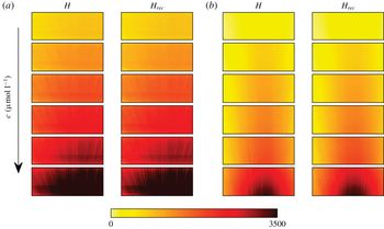
PLIF quantification is usually performed under the linearity assumption, i.e. the observed intensity of the fluorescent light is considered proportional to the local PLIF tracer concentration. There are a number of successful studies that used these assumptions (e.g. Walker (Reference Walker1987) or Crimaldi (Reference Crimaldi2008)). Nevertheless, this approach can be unsatisfactory if very high local concentrations of the tracer occur or if the illumination light attenuation is strong. Since these particular conditions are present in this study due to high initial rhodamine concentration released into the flow (this was necessary given the particularly high dispersion rate in the vicinity of the frame) a nonlinear quantification technique is required. A suitable technique, that is followed in the present study, was proposed by Baj et al. (Reference Baj, Bruce and Buxton2016).
 $$\begin{eqnarray}\displaystyle H=h\left(\text{Const}\cdot \frac{\unicode[STIX]{x1D6FE}Qc\unicode[STIX]{x1D719}(c)}{r\unicode[STIX]{x1D712}}\exp \left(-\unicode[STIX]{x1D716}\int _{r_{0}}^{r}c\,\text{d}\unicode[STIX]{x1D701}\right)\right). & & \displaystyle\end{eqnarray}$$
The PLIF measurement model proposed in Baj et al. (Reference Baj, Bruce and Buxton2016) is given by equation (3.1) where the particular variables stand for:
 $H$
– the acquired image,
 $h$
– the camera’s transfer function,
 $\unicode[STIX]{x1D6FE}$
– the illumination energy profile,
 $Q$
– the optics transfer rate,
 $c$
– local concentration level,
 $\unicode[STIX]{x1D719}$
– quantum yield,
 $r$
– the radial coordinate (of the polar coordinate system whose origin coincides with the laser sheet’s origin;
 $r_{0}$
stands for the coordinate of the flume’s floor, see figure 6),
 $\unicode[STIX]{x1D712}$
– the secondary fluorescence contribution and
 $\unicode[STIX]{x1D716}$
– extinction coefficient (i.e. the rate of illumination attenuation). Note that all of these quantities (except for
 $\unicode[STIX]{x1D716}$
) are actually functions of spatial position. Additionally, the local read-out
 $H$
depends on the concentration’s integral along the radial coordinate (which coincides with the illumination ray).
The secondary fluorescence concept was initially proposed by Vanderwel & Tavoularis (Reference Vanderwel and Tavoularis2014) and further discussed in Baj et al. (Reference Baj, Bruce and Buxton2016). Generally, it assumes that, on top of the original laser illumination, a patch of dye is further excited by the fluorescent light emitted in its vicinity. This causes a non-local self-amplification effect that significantly alters PLIF measurements in areas of high concentration gradients which can easily be visualised as a ‘halo’ surrounding localised regions of high concentration. It is proposed by Baj et al. (Reference Baj, Bruce and Buxton2016) to model this additional illumination with a convolution of the primary fluorescence intensity field (i.e. the fluorescence intensity that would have been observed if no self-amplification was present) with a spatial kernel that decays as
 $x^{-a}$
(where
 $x$
is a spatial coordinate and
 $a$
is a positive constant).
Equation (3.1) can be solved for
 $c$
given
 $h$
,
 $\unicode[STIX]{x1D719}$
,
 $a$
and
 $\unicode[STIX]{x1D716}$
are known. Additionally, a background image
 $H_{b}$
is required, i.e. a PLIF image of a uniform dye concentration field
 $c_{b}$
, taken with the exact same optical set-up. The tank experiment’s purpose was to extract these required characteristics and to provide
 $H_{b}$
. One also needs to make the following assumptions:
(i) The camera’s transfer function
 $h$
is a monotonic increasing function that satisfies
$h(0)=0$
.
(ii)
$h$
,
$\unicode[STIX]{x1D6FE}$
and
$\unicode[STIX]{x1D64C}$
are time invariant parameters of the particular set-up.(iii)
$\unicode[STIX]{x1D719}$
is a concentration function specific to the experimental conditions, that can be approximated with
$b_{1}(c-b_{2})^{b_{3}}/c$
(
$b_{i}$
being real parameters, see Baj et al. (Reference Baj, Bruce and Buxton2016)).(iv)
$\unicode[STIX]{x1D716}$
and
$a_{i}$
are constant and specific to the experimental conditions.


Camera transfer functions resolved in (a) experiment 2, (b) experiment
 $3$
, (c) quantum yield – concentration dependence, (d) profiles of illumination intensity.

The exact solution method is complex and multi-step and thus is not described here. All the details can be found in Baj et al. (Reference Baj, Bruce and Buxton2016). Nevertheless, let us present the characteristics inferred from the tank experiments. Figure 5(a,b) shows functions
 $h$
evaluated for experiments
 $2$
and
 $3$
respectively. These two are nearly the same (which could have been expected given similar experimental conditions). The transfer functions deviate from linearity by less than
 $10\,\%$
for the argument values larger than approximately
 $1100$
pixel intensity counts above zero. Figure 5(c) presents the quantum yield dependency on the concentration value. Almost identical characteristics are observed in both quantitative experiments. Figure 5(d) shows the illumination intensity profiles
 $\unicode[STIX]{x1D6FE}$
. These are plotted against the angular coordinate of the polar coordinate system originating at the laser sheet’s origin (see figure 6). The exponent
 $a$
of the secondary fluorescence kernel spans an interval 1.13–1.27, depending on the experiment and the measurement station. Note that this coefficient is evaluated separately for each downstream position, unlike the remaining quantities. Finally, the extinction coefficient is found to be equal to
 $8520~\text{l}~(\text{mm}~\text{mol})^{-1}$
and
 $7950~\text{l}~(\text{mm}~\text{mol})^{-1}$
for experiments
 $2$
and
 $3$
respectively.
Schematic showing the position of the polar coordinate system associated with the laser sheet.

Equation (3.1) allows evaluation of a concentration field based on the image but it can also be used in a reversed manner, i.e. the image can be reconstructed given the known concentration field. It is particularly easy for the calibration images as the concentration fields are uniform. Figure 7 presents the original calibration images compared to the reconstructed ones for a number of different concentrations levels. As can be seen, the corresponding images are nearly identical. Close inspection reveals that the differences do not exceed
 $4\,\%$
and
 $2\,\%$
for experiments
 $2$
and
 $3$
respectively. This indicates that the quantification is successful.
Original (a) and reconstructed (b) calibration images for different concentration values: (a) experiment
 $2$
, (b) experiment
 $3$
.

The ultimate test of the quantification quality would be evaluation of the scalar’s mass flow rate
 $\dot{q}_{m}$
and comparison against its known value of
 $\dot{q}$
(see table 2). Simultaneous information about velocity and concentration fields at a cross-stream plane is required for this purpose. This is not available in the present work, however, one can make a reasonable approximation of the mass flow rate by making some assumptions. First, let us assume that the mean streamwise velocity is constant along the spanwise directions around the channel’s mid-plane (within the FOV of experiment 2, i.e.
 $z/H=\pm 0.06$
). This can be justified by the fact that the aspect ratios of the bars are high (the aspect ratio of the big bar equals
 $7.6$
). The mass flow rate can now be approximated by integrating a product of the mean concentration field captured in experiment
 $2$
(these are shown explicitly in § 4) and the transverse mean velocity profiles resolved in experiment
 $3$
. Note that this neglects the contribution from the fluctuations’ product, however, these are believed to be negligible (the approximation based on experiment
 $2$
suggests its relative contribution does not exceed
 $2\,\%$
). Further, in order to approximate the mass flow rate based on the concentration results of experiment
 $3$
, one can assume that the shape of the cross-stream distribution of the mean concentration changes linearly between the downstream positions surveyed in experiment
 $2$
. By scaling this shape according to the concentration transverse profiles measured in experiment
 $3$
, the mass flow rate can be resolved. Figure 8 provides the results of these described calculations.
PLIF based estimation of the scalar’s mass flow rate based on experiments
 $2$
and
 $3$
(the label ‘no s.f.’ denotes results neglecting the contribution of secondary fluorescence).

Experiment
 $2$
shows a systematic decrease of the recovered mass flow rate. This is mainly due to the limited size of its FOV (a considerable part of non-zero mean concentration distribution exceeds the FOV’s boundaries). Experiment
 $3$
, on the other hand, had a larger FOV (see table 2) and thus the mass flow rate is better recovered,
 $\dot{q}_{m}/\dot{q}$
is roughly constant and equals
 $0.88$
on average. The deviation from unity can also be attributed to approximations and assumptions taken during the mass flow rate’s evaluation as well as to different sources of uncertainty (e.g. PLIF uncertainty, PIV uncertainty, laser energy measurement uncertainty, initial concentration uncertainty etc.). This is not the perfect result, however, it is an improvement in comparison to Vanderwel & Tavoularis (Reference Vanderwel and Tavoularis2014), who reported values of the order of
 $0.7$
at a comparable position downstream of the scalar point source (i.e. normalised with the channel cross-section size). It is worth noting that by considering the secondary fluorescence correction the mass flow rate approximation has improved considerably (see figure 8). If no secondary fluorescence correction was introduced,
 $\dot{q}_{m}/\dot{q}$
averaged would reach a value of
 $0.60$
(based on experiment
 $3$
).
4 Results
Let us start with an overview of some general characteristics of our considered flows. Figure 9 shows the basic single point statistics of the velocity fields resolved in experiment
 $1$
for the multi- and single-scale cases. The mean streamwise velocity field
 $\bar{u}_{1}$
is highly inhomogeneous, as can be seen in figure 9(a). A prolonged recirculation area can be distinguished behind the largest bar that reaches almost
 $5t^{I}$
, whilst significantly shorter recirculations are present behind the remaining two. A sizable deflection of the smaller wakes is present, outwards from the centreline (outwards and inwards directions are understood hereafter as pointing towards the centreline and towards the floor respectively). Figure 9(b) shows the associated turbulence intensity field
 $I_{T}=\sqrt{0.5(u_{1}^{\prime 2}+u_{2}^{\prime 2})}/U_{\infty }$
. Again, there is a qualitative difference between the appearances of the biggest wake and the remaining wakes. In the latter case the local maxima are located closely downstream of particular bars, whereas in the big bar’s case the peak is postponed to significantly downstream relative to the expected position for a single comparable bar (see Okajima Reference Okajima1982). The cross marks denote adjacent wake intersection points. Following Baj & Buxton (Reference Baj and Buxton2017), these are defined as points located between two neighbouring wakes, where spatial gradients of the turbulence intensity field vanish. Note that this definition does not exactly match the wake intersection definition postulated in Mazellier & Vassilicos (Reference Mazellier and Vassilicos2010) which was given in the context of the grid’s geometry rather than the actual velocity field topology. The exact locations of the recognised intersection points are
 $(x/H,y/H)=\{(0.22,-0.33),(0.57,-0.25)\}$
. The shedding frequencies of particular bars are evaluated to be 0.4 Hz, 2.4 Hz, 5.9 Hz for the largest to smallest bars (they are referred to as
 $f^{I}$
,
 $f^{II}$
,
 $f^{III}$
respectively); the shedding frequencies are evaluated based on locations of spectral peaks in power density spectra of the velocity field resolved from experiment
 $1$
(the Welch method, see Welch (Reference Welch1967), with Hann windowing used). The affiliated Strouhal numbers are
 $0.16$
,
 $0.30$
,
 $0.28$
(note that
 $U_{\infty }$
is used as the velocity scale when evaluating Strouhal numbers).
Mean streamwise velocity
 $\bar{u}_{1}$
and turbulence intensity
 $I_{T}$
in flows past (a,b) the multi-scale array and (c,d) the single-scale array. The cross marks indicate the wake intersection points (based on experiment
 $1$
).

The flow past the single-scale array is illustrated by figure 9(c,d). Despite using the same bars across the uniform array, the resultant wakes are not strictly similar. In particular, the bottom wake’s behaviour deviates from the others. One can speculate that this is due to the boundary layer vicinity or maybe a Coandă effect induced by the streamlining element attached to the outer frame. Nevertheless, the remaining three wakes are quite similar, as one might expect in the single-scale arrangement, and the present work focuses on these. Generally speaking, the resultant mean streamwise velocity and the turbulence intensity fields recover homogeneity quicker compared to the multi-scale case. The turbulence intensity peaks just past the bars (except for the bottom one). The wake intersection points are located at
 $(x/H,y/H)=\{(0.16,-0.01),(0.17,-0.14),(0.28,-0.27)\}$
. In agreement with Laizet & Vassilicos (Reference Laizet and Vassilicos2012), intersections of similar wakes occur at roughly the same downstream location. The shedding frequencies of the particular bars are evaluated to be 1.1 Hz, 1.9 Hz, 1.8 Hz, 1.8 Hz for the bottom to the top bars (these are calculated in a similar manner as in the multi-scale case). The respective
 $St$
are
 $0.14$
,
 $0.23$
,
 $0.22$
,
 $0.22$
. Transient periods of synchronisation between sheddings from neighbouring bars are observed. This can be illustrated with a probability density function (PDF) of a phase lag
 $\unicode[STIX]{x1D6E5}_{\unicode[STIX]{x1D711}}$
between vorticity signals measured at the centres of adjacent wakes of the single-scale array shown in figure 10. Note that anti-phase synchronisation (
 $\unicode[STIX]{x1D6E5}_{\unicode[STIX]{x1D711}}=\unicode[STIX]{x03C0}$
) is preferred over in-phase synchronisation (
 $\unicode[STIX]{x1D6E5}_{\unicode[STIX]{x1D711}}=0$
), although this tendency is stronger farthest upstream and its weakening is particularly evident at the farthest checked downstream location.
Phase lags
 $\unicode[STIX]{x1D6E5}_{\unicode[STIX]{x1D711}}$
between vorticity signals measured at the centres of adjacent wakes of the single-scale array at various downstream locations (based on experiment
 $1$
).

All the above observations are consistent with the previous findings reported in Baj & Buxton (Reference Baj and Buxton2017). Since the cited work provides a thorough discussion of these results, let us skip further interrogation of the velocity field. Still, it is worth noting that the observed differences between single- and multi-scale arrays are qualitatively similar to some of those seen between FGs and RGs (see Laizet & Vassilicos Reference Laizet and Vassilicos2012; Melina, Bruce & Vassilicos Reference Melina, Bruce and Vassilicos2016). In particular, the turbulence intensity’s streamwise decay is much more rapid in the multi-scale array case (i.e. in the sense of the transverse-averaged turbulence intensity’s slope when plotted against the streamwise coordinate
 $x$
), homogeneity recovery is slower and the wake intersection point streamwise positions are scattered. Preservation of these characteristics provides some confidence in extrapolation of the qualitative findings reported in the present work onto cases with more complex multi-scale geometry.
4.1 Qualitative PLIF results
The PLIF measurements of experiment
 $1$
provide initial, qualitative insight into the scalar behaviour when released into the studied flows. In general, scalar tends to accumulate around the shed vortices and is convected downstream along with them. Nevertheless, the further downstream the more chaotic the concentration field gets and the wider it spreads. This could have been expected as similar qualitative observations were reported by e.g. Williamson (Reference Williamson1985) and Sumner (Reference Sumner2010). Interestingly, however, quasi-periodic scalar transport events were spotted in the flows. These events can be described as transverse-elongated, large-scale scalar structures which emerge from a scalar-containing wake. These will be referred to as scalar bursts/bursting hereafter. A representative sequence of PLIF images acquired in the flow past the multi-scale array is shown in figure 11(a) on top of the turbulence intensity isolines, indicating the wake positions. Three consecutive bursts are highlighted with arrows. It appears from an analysis of these qualitative data that these surges start to emerge from the small wake roughly at
 $x/H=0.2$
. This coincides with the wakes’ intersection point between the medium and small wakes (see figure 9
b). The scalar is lifted quasi-periodically and seems to be entrained into the adjacent wake, judging by the turbulence intensity contours. It is worth noting that this matches the SSU concept almost exactly.
Sequences of consecutive qualitative PLIF images acquired at times
 $t$
downstream of (a) the multi-scale array (b,c) the single-scale array on top of the turbulence intensity isolines (black contour). Blue arrows highlight positions of transverse scalar bursts (based on experiment
 $1$
, the related animations are uploaded as supplementary material is available online at https://doi.org/10.1017/jfm.2019.11).
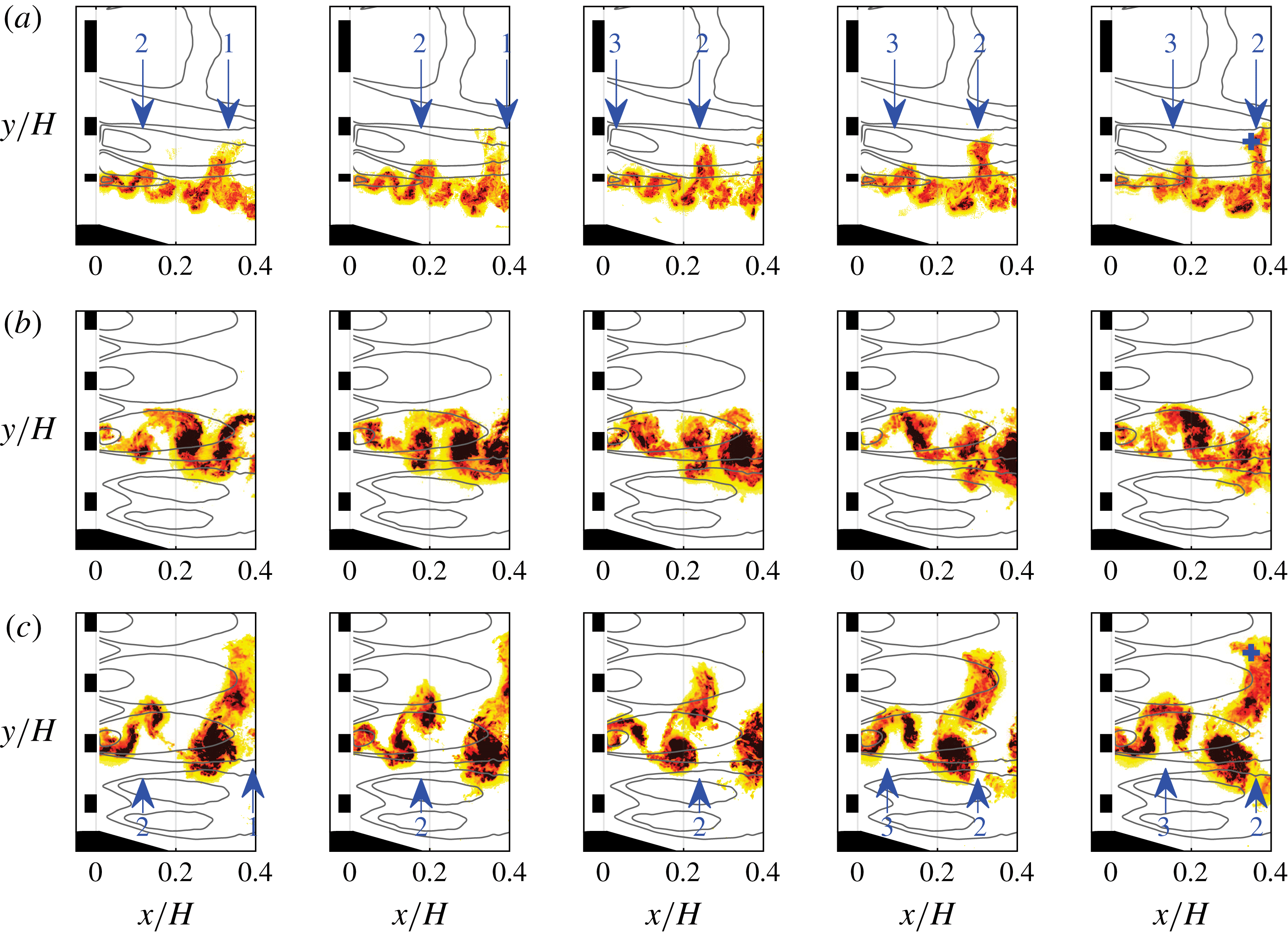
Figure 11(b,c) shows PLIF image sequences corresponding to the flow past the single-scale array. Unlike previously, one could recognise relatively long time intervals when no bursting occurs (figure 11
b) as well as those when bursting is present (figure 11(c); bursts are highlighted with arrows). The transverse extent of the bursts depicted in figure 11(c) is even larger than in the multi-scale flow. Also in this case the burst’s initiation seems to coincide with wake intersection. Note that during the bursting suppression period the dye appears to be trapped inside the bounds of its original wake. The local PLIF image intensity at the spatial position marked with a blue cross on the right-hand figure 11(c) can be utilised to identify burst occurrence. Although the selection of this particular spatial spot is highly arbitrary, it still gives us some indication of how often bursting occurs. The temporal evolution of the signal is shown in figure 12(a). Each of the present peaks can be associated with a single burst event. Fifty flips between bursting/suppression were recognised within the studied dataset. The mean duration of the bursting period equals
 $\overline{\unicode[STIX]{x0394}t}f^{II}=2.76$
, whilst the mean duration of the suppression period can be estimated as
 $\overline{\unicode[STIX]{x0394}t}f^{II}=3.46$
. Unfortunately, the sample is not large enough to reliably investigate the underlying distributions of the durations of the bursting/suppresion events (although the data seemed to be relatively well fitted with an exponential distribution). Note that suppression is dominant over bursting in this case, as opposed to the stable bursting observed past the multi-scale array depicted in figure 12(b) (the signal probing location is indicated with a blue cross in the on the right-hand figure 11
a). This bi-stable behaviour of the single-scale flow is not accounted for by the original SSU description.
Temporal evolution of the PLIF intensity signal recorded in the flow past: (a) the single-scale array, (b) the multi-scale array. The signals are probed at the spatial positions indicated by blue cross marks respectively in figure 11(c,a) (the last image of the sequence, based on experiment 1).

The key concept of the SSU mechanism is that the fluid exchange between wakes is intensified at each intersection occurrence. Figure 11 provides examples of dye transfers spotted in the vicinity of the closest downstream intersection point. A similar behaviour can be noticed around the second intersection point in the multi-scale case (i.e.
 $x/H=0.57$
), which is presented in figure 13. It is quite clear that some dye patches are entrained into the biggest wake area (designated by the turbulence intensity contours). A closer inspection of the gathered qualitative data shows that a dye patch which first entered the medium wake around
 $x/H=0.2$
is often lifted further towards the big wake past
 $x/H=0.5$
. Alternatively, a burst can go directly from the smallest to the biggest wake, however, this is seen less frequently and also seems to happen further downstream (although it is hard to identify any precise position based on the considered dataset). It is intuitively consistent that given a larger separation between the smallest and biggest wake (compared to the medium–biggest separation), the bursting is postponed downstream.
On the other hand, in the single-scale case it was hardly possible to recognise any subsequent transverse bursts past the intersection point at
 $x/H=0.16{-}0.17$
. The general impression created by considering the instantaneous concentration field behaviour downstream of the intersection point is that the scalar tracer is simply convected at scales comparable with the size of the bursts. As a consequence, the bursts are observable at all the following downstream positions. However, their transverse transport seems inhibited in comparison to the multi-scale case.
A qualitative PLIF image acquired in the flow past the multi-scale array on top of the turbulence intensity isolines (black contour). The blue arrow indicates a transverse burst occurring between the medium and the big wake.

Summarising the qualitative results, it seems that the SSU idea is a quite accurate description of the observed phenomenology. Indeed, a fluid particle which is initiated in a certain wake is likely to be engulfed into another larger wake when these two intersect. Moreover, a series of consecutive inter-wake transfers is present when the intersections of different wakes occur at various streamwise locations, i.e. unfold in space. On the other hand, Laizet & Vassilicos (Reference Laizet and Vassilicos2012) did not foresee that the inter-wake transfer of scalar can be transiently suppressed in the case of same-size wakes interaction.
4.2 Quantitative PLIF results
Let us now focus on the quantitative results of experiments
 $2$
and
 $3$
, which focus on the area around the near-downstream wake intersection point (i.e.
 $x/H=0.22$
). These enable quantitative assessment of basic statistics of the scalar dispersion in the flow past the multi-scale array (in the context of which the SSU mechanism is postulated). The impact of the bursting on concentration mean and r.m.s. fields (denoted as
 $\bar{c}$
and
 $c_{rms}$
respectively) can be assessed from figure 14. The statistics are evaluated at three different cross-stream planes. The transverse profiles (i.e. along the
 $y$
direction) are noticeably skewed towards positive values of
 $y$
, except for the closest downstream case which stays roughly symmetric against the point of maximum value. This inclination, however, is an anticipated consequence of the observed bursting. The skewness of an arbitrary transverse profile
 $c(y)$
can by quantified with the parameter
 $\unicode[STIX]{x1D6FE}_{c}$
defined as (
 $y_{c}$
and
 $\unicode[STIX]{x1D70E}_{c}$
represent the profile’s centre position and width measure respectively):
 $$\begin{eqnarray}\displaystyle \unicode[STIX]{x1D6FE}_{c}=\frac{\displaystyle \int _{-H/2}^{H/2}c(y)(y-y_{c})^{3}\,\text{d}y}{\displaystyle \unicode[STIX]{x1D70E}_{c}^{3}\int _{-H/2}^{H/2}c(y)\,\text{d}y},\quad y_{c}=\frac{\displaystyle \int _{-H/2}^{H/2}c(y)y\,\text{d}y}{\displaystyle \int _{-H/2}^{H/2}c(y)\,\text{d}y},\quad \unicode[STIX]{x1D70E}_{c}=\sqrt{\frac{\displaystyle \int _{-H/2}^{H/2}c(y)(y-y_{c})^{2}\,\text{d}y}{\displaystyle \int _{-H/2}^{H/2}c(y)\,\text{d}y}}. & & \displaystyle \nonumber\\ \displaystyle & & \displaystyle\end{eqnarray}$$
The values of
 $\unicode[STIX]{x1D6FE}_{\bar{c}}$
equal
 $0.16$
,
 $0.59$
and
 $0.61$
for
 $x/H=0.21,0.33,0.45$
. The values of
 $\unicode[STIX]{x1D6FE}_{c_{rms}}$
, on the other hand, are found to be approximately
 $0.21$
,
 $0.37$
,
 $0.41$
respectively. The spanwise profiles are hardly affected by the bursting and stay almost exactly Gaussian at all the considered locations.
Mean concentration fields at
 $x/H=$
(a)
 $0.21$
, (b)
 $0.33$
, (c)
 $0.45$
and concentration fluctuation r.m.s. field at
 $x/H=$
(d)
 $0.21$
, (e)
 $0.33$
, (f)
 $0.45$
in the flow past the multi-scale array (based on experiment
 $2$
).

Statistics of the flow past the multi-scale array: (a) mean concentration field, (b) concentration fluctuation r.m.s. field, (c) centres of the statistics transverse profiles
 $y_{c}$
, (d) skewness of the statistics transverse profiles
 $\unicode[STIX]{x1D6FE}_{c}$
and (e) ratio of widths of the statistics transverse profiles
 $\unicode[STIX]{x1D70E}_{c_{rms}}/\unicode[STIX]{x1D70E}_{\bar{c}}$
(based on experiment
 $2$
).

Note that the area of non-zero mean concentration exceeds the FOV’s boundaries downstream of the first downstream station as shown in figure 14. This is mainly due to the positive transverse skewness but also due to spanwise growth. The shapes of these transverse mean concentration distributions were used to estimate the scalar’s mass flow rate shown in figure 8. The under prediction of the flow rate to some extent might be the result of some scalar being transported beyond the confines of the limited FOV size, evident from figure 14. Areas of non-zero r.m.s. values are even broader, in particular they extend to below the lower FOV’s edge as well as exceed the side edges. This could have affected the quantification of experiment
 $2$
to some extent as whatever attenuation occurred below the FOV, it is not accounted for in the utilised quantification routine.
Figure 15 provides counterpart results of experiment
 $3$
. In this case the FOV’s transverse extent is large enough to cover the entire non-zero areas of the mean and r.m.s. concentration fields. The transverse widths of the statistics profiles (i.e.
 $6\unicode[STIX]{x1D70E}$
) grow linearly with the streamwise position, starting from
 $0.10H$
and
 $0.12H$
at
 $x/H=0.12$
up to
 $0.31H$
and
 $0.39H$
at
 $x/H=0.48$
respectively for
 $\bar{c}$
and
 $c_{rms}$
. The inwards shift (i.e. towards the centre-line) of the statistics is also very clear in figure 15. In order to quantify this tendency, let us consider the streamwise behaviour of the profile parameters. Figure 15(c) presents
 $y_{c}$
for the mean and r.m.s. fields. In both cases, quite abrupt change can be seen at around
 $x/H=0.2{-}0.25$
. Upstream of this spot the centre locations move outwards (i.e. away from the centreline) whilst they start to move inwards downstream of this point. Note that the spatial location of this change coincides with the position of the wakes’ intersection point. This indicates that the bursting events are triggered by the wakes intersection. Similar observations can be made in the context of
 $\unicode[STIX]{x1D6FE}_{c}$
. Initially, the values grow from
 $0$
to settle at a level of
 $0.6$
and
 $0.4$
for
 $\bar{c}$
and
 $c_{rms}$
roughly past the intersection point. Finally, although the growths of the profile widths
 $\unicode[STIX]{x1D70E}_{c}$
is linear, as mentioned before, the ratio
 $\unicode[STIX]{x1D70E}_{c_{rms}}/\unicode[STIX]{x1D70E}_{\bar{c}}$
peaks at
 $x/H=0.26$
, which again coincides with the wake intersection position.
The transverse turbulent scalar flux
 $\overline{c^{\prime }u_{2}^{\prime }}$
is observed by Laizet & Vassilicos (Reference Laizet and Vassilicos2012) to be highly enhanced in flows past fractal (multi-scale) grids compared to regular (single-scale) grids. Let us, therefore, examine
 $\overline{c^{\prime }u_{2}^{\prime }}$
in our considered case, which is presented in figure 16. The inwards transport is noticeably more intense, even at initial downstream locations. Initially only
 $28\,\%$
of the transverse integral of
 $\overline{c^{\prime }u_{2}^{\prime }}$
is directed outwards. This value decays to approximately
 $12\,\%$
at
 $x/H=0.33$
and downstream of this point it stays constant. The correlation between the concentration and velocity fluctuations is initially higher (in an absolute sense) in the outer branch of the wake, its absolute value exceeds
 $0.4$
. However, the maximum correlation value within the outer branch decreases along the streamwise direction, reaching a value of
 $-0.25$
at the final station. On the other hand, the maximum correlation observed in the inner part is roughly constant along the streamwise extent and equal to
 $0.32$
. An equal correlation level between two branches is reached roughly at
 $x/H=0.22$
. These correlation levels can be compared against corresponding results provided by Matsumura & Antonia (Reference Matsumura and Antonia1993) in the context of a flow past a circular heated cylinder at the diameter-based Reynolds number of
 $5830$
. The authors reported anti-symmetric profiles of
 $\overline{c^{\prime }u_{2}^{\prime }}$
with the maximum absolute correlation level increasing from roughly
 $10\,\%$
to
 $25\,\%$
at the initial and final downstream locations of the present work. On the other hand, results of a Large Eddy Simulation (LES) of a flow past a rectangular prism, with a point-wise scalar release located half a diameter past the rear prism’s face, reported by Lodato & Rossi (Reference Lodato and Rossi2013) suggests a correlation of the order of
 $35\,\%$
even upstream of the initial section of the present work. In the case of both studies, however, the flux was not directed towards any particular side (i.e. inwards or outwards) as opposed to the current work. Zhou, Zhang & Yiu (Reference Zhou, Zhang and Yiu2002) reports a qualitatively similar bias of the transverse scalar flux in the case of a flow past two circular cylinders operating in the two-frequency regime (i.e. vortices are shed from particular bars at different frequencies despite identical diameters;
 $Re=5800$
).
(a) The absolute value of the transverse turbulent scalar flux and (b) correlation between the transverse velocity fluctuations and concentration fluctuations.

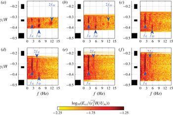
Finally, the spectral content of the concentration fluctuations is shown in figure 17. Different spectral peaks are observed at different downstream positions, however, those located at
 $f^{II}$
and
 $f^{III}$
are usually dominant. Except for those, there are also noticeable contributions from their harmonics at a few downstream locations. Interestingly, the peak at
 $f^{II}$
appears within the wake of the small bar (although this is the shedding frequency of the medium bar). At the initial position it coexists within the inner wake’s half with the peak at
 $f^{III}$
(figure 17
a) but downstream of
 $x/H=0.30$
, the peak
 $f^{III}$
is absent from the inner wake’s part. At the same time the outer part is still characterised by frequency
 $f^{III}$
exclusively. These spectral properties suggest that the bursting occurs at the shedding frequency of the medium bar. The limited transverse extent of the peak
 $f^{II}$
indicates that the bursting involves only the inner part of the wake. The rapid extinction of the
 $f^{III}$
peak coincides with the wakes’ intersection point location (i.e.
 $x/H=0.22$
).
Power spectral densities (PSDs) of concentration fluctuations in the flow past the multi-scale array evaluated at
 $x/H=$
(a)
 $0.12$
, (b)
 $0.18$
, (c)
 $0.24$
, (d)
 $0.30$
, (e)
 $0.36$
, (f)
 $0.42$
. Arrows indicate the positions of prominent spectral peaks (based on experiment
 $3$
).

Similar spectral analysis regarding the velocity field is reported by Baj & Buxton (Reference Baj and Buxton2017). Relatively strong secondary peaks residing at
 $f^{III}\pm f^{II}$
were recognised by the authors in addition to the primary shedding frequencies
 $f^{II}$
and
 $f^{III}$
. The associated secondary coherent motions were at their most energetic in the vicinities of the wake intersection points. The interrogation of the triple-decomposed energy budget performed by Baj & Buxton (Reference Baj and Buxton2017) showed that these secondary coherent motions are products of triadic interactions between the primary shedding motions. In particular, the low-frequency secondary fluctuations drain energy mostly from the high-frequency primary motion. It was speculated that this is the reason why the latter is observed to be less spatially persistent than the low-frequency secondary coherent motion. Contrastingly, the primary shedding motions are driven by the mean flow. Nothing similar can be seen in the case of the concentration PSD, i.e. at least not at a comparable level. This suggests that the energetic secondary coherent velocity motions are not directly important to the scalar transport. Nevertheless, they might be indirectly meaningful due to their mutual interactions with the primary shedding structures (in the context of the velocity field) since the latter are of the primary importance to the scalar transport.
4.3 Triple decomposition
Further insight into the studied flow’s physics can by brought by introducing the triple decomposition, as originally suggested by Hussain & Reynolds (Reference Hussain and Reynolds1970). This is fully justified in the context of the present flow, as particularly strong coherent fluctuations (manifesting themselves as spectral peaks in the PSDs) coexist with stochastic turbulent fluctuations. Let us, therefore, decompose an arbitrary field
 $a(\boldsymbol{x},\unicode[STIX]{x1D70F})$
into its temporal mean
 $\bar{a}$
, a number of coherent contributions associated with particular spectral peaks
 $\tilde{a}^{l}$
and the residual stochastic part
 $a^{\prime \prime }$
(
 $\boldsymbol{x}$
stands for a spatial coordinate and
 $\unicode[STIX]{x1D70F}$
represents time). This can be written as equation (4.2).
 $$\begin{eqnarray}\displaystyle a(\boldsymbol{x},\unicode[STIX]{x1D70F})=\bar{a}(\boldsymbol{x})+a^{\prime }(\boldsymbol{x},\unicode[STIX]{x1D70F})=\bar{a}(\boldsymbol{x})+\mathop{\sum }_{l}\tilde{a}^{l}(\boldsymbol{x},\unicode[STIX]{x1D70F})+a^{\prime \prime }(\boldsymbol{x},\unicode[STIX]{x1D70F}). & & \displaystyle\end{eqnarray}$$
The implementation of triple decomposition is not trivial and there are a number of different methods for performing it (e.g. Hosseini, Martinuzzi & Noack Reference Hosseini, Martinuzzi and Noack2016). A method introduced by Baj et al. (Reference Baj, Bruce and Buxton2015) and further extended in Baj & Buxton (Reference Baj and Buxton2017) is utilised in the present study (this decomposition technique allows an efficient segregation of fluctuations associated with particular wakes despite pronounced differences in energy levels). It relies on the optimal mode decomposition (OMD, see Wynn et al. (Reference Wynn, Pearson, Ganapathisubramani and Goulart2013)), i.e. the complex OMD modes
 $\unicode[STIX]{x1D6F7}$
that link to particular coherent fluctuations are recognised. Further, by projecting fluctuations onto the basis spanned by the selected modes, a set of complex projection coefficients is yielded. Their arguments can be interpreted as the instantaneous phase signal
 $\unicode[STIX]{x1D719}^{l}$
associated with the corresponding coherent mode, whereas their magnitudes represent the instantaneous modulation
 $A^{l}$
. Ultimately, coherent fluctuations
 $\tilde{a}^{l}$
can be represented as equation (4.3) (
 $\text{}\underline{a}$
represents the complex conjugate of
 $a$
).
 $$\begin{eqnarray}\displaystyle \tilde{a}^{l}(\boldsymbol{x},\unicode[STIX]{x1D70F})=A^{l}(\unicode[STIX]{x1D70F})(\unicode[STIX]{x1D6F7}(\boldsymbol{x})\exp (\text{i}\unicode[STIX]{x1D719}^{l}(\unicode[STIX]{x1D70F}))+\text{}\underline{\unicode[STIX]{x1D6F7}}(\boldsymbol{x})\exp (-\text{i}\unicode[STIX]{x1D719}^{l}(\unicode[STIX]{x1D70F}))). & & \displaystyle\end{eqnarray}$$
The stochastic fluctuations are evaluated simply as the residual of the total fluctuations once the coherent parts are subtracted (they should not be confused for some kind of uncorrelated random signal). Some further details of the utilised triple-decomposition technique are introduced in appendix A along with some example decompositions. More extensive characterisation can be found in the original work of Baj et al. (Reference Baj, Bruce and Buxton2015).
Energies of normalised coherent velocity modes associated with frequencies (a)
 $f^{II}$
, (c)
 $f^{III}-f^{II}$
, (e)
 $f^{III}$
, (g)
 $f^{III}+f^{II}$
and variances of normalised coherent concentration modes associated with frequencies (b)
 $f^{II}$
, (d)
 $f^{III}-f^{II}$
, (f)
 $f^{III}$
, (h)
 $f^{III}+f^{II}$
.

Let us start with an overview of the extracted coherent modes
 $\unicode[STIX]{x1D6F7}$
. Figure 18 presents the normalised energy and variance associated with the resolved velocity and concentration modes. Following Baj & Buxton (Reference Baj and Buxton2017), primary and secondary coherent modes are recognised. The velocity modes are unsurprisingly similar to those reported in the cited work. The counterpart concentration modes are relatively clearly defined in the case of the primary coherent motions (figure 18
b,f), whereas they are less defined in the secondary coherent motion cases (figure 18
d,h). This can be explained by the fact that the energy content of the secondary coherent fluctuations is negligible, as reported in table 5. The maximum local contribution to the total concentration variance does not exceed
 $1\,\%$
within the FOV. Therefore, the secondary coherent modes are likely polluted with relatively intense noise and so the appearance of the normalised modes is rather vague. Additionally, it follows from table 5 that the extracted modes are in general much more representative of the velocity field than of the concentration field. Similar conclusions are reached by Matsumura & Antonia (Reference Matsumura and Antonia1993), Lodato & Rossi (Reference Lodato and Rossi2013) who also performed a triple decomposition of concentration and velocity fields in the near wake of a bar. In both cases the authors observed the contribution of the coherent fluctuations to the total concentration variance to be approximately
 $20\,\%$
of the relative level. On the other hand, the contribution of coherent fluctuations to the variance of the transverse velocity fluctuations reached beyond
 $70\,\%$
in the study of Matsumura & Antonia (Reference Matsumura and Antonia1993). Although this is not an exact match with the present results (which in any case is unexpected), similar tendencies are observed between the current results and these previous findings.
Maximum local contributions of coherent velocity fluctuations to the total energy and maximum local contributions of coherent concentration fluctuations to the concentration variance (based on experiment
 $3$
).

The shape of the concentration mode associated with
 $f^{III}$
consists of two separate branches. Until approximately
 $x/H=0.17$
the branches are of equal strength. However, the inwards part starts vanishing rapidly downstream of this streamwise position and diminishes below
 $0.01$
(in the sense of the normalised mode’s local value) roughly at the wake intersection point. The outwards branch, on the other hand, reaches the same magnitude level around
 $x/H=0.30$
. The mode associated with
 $f^{II}$
consists of a singular branch only. Its edge at the inner side coincides with the small wake’s centreline, which is consistent with the previously presented PSDs (i.e. the peak
 $f^{II}$
does not extend into the outer half of the small wake).
The absolute value of transverse scalar flux induced by (a) coherent fluctuations associated with frequency
 $f^{II}$
, (b) coherent fluctuations associated with frequency
 $f^{III}$
, (c) stochastic fluctuations and (d) ratio between transverse integrals of the particular flux components and the total flux.

Having decomposed the fluctuations into coherent and stochastic parts, it is possible to study their influence on the total transverse scalar flux. The most significant contributions are depicted in figure 19 (note that the secondary coherent modes are omitted as their magnitudes are negligible). The primary coherent motions are, on the other hand, of the primary importance. Figure 19(d) presents a metric quantifying the contributions of the recognised fluctuation components to the total flux (i.e. the ratio between transverse integrals of the absolute value of the total flux and that of the components). The fluctuations associated with
 $f^{II}$
are responsible for the majority of the scalar flux roughly past the wakes’ intersection point. Spatially, their contribution is restricted to the inwards side of the small wake (see figure 19
a). The contribution from
 $f^{III}$
oscillates around
 $10\,\%$
upstream of the wakes’ intersection point, whilst it gradually decays past this point. In this case the outwards branch is mostly affected (see figure 19
b). The importance of the stochastic fluctuations is retained throughout the streamwise extent at a relatively high level (above
 $40\,\%$
). Matsumura & Antonia (Reference Matsumura and Antonia1993) reported similar statistics. The contribution from the coherent fluctuations was reported to decrease from
 $68\,\%$
down to
 $43\,\%$
at the downstream locations comparable to the initial and the final downstream stations of the present work. The share of roughly
 $50\,\%$
can be inferred from the data shown in Lodato & Rossi (Reference Lodato and Rossi2013) (at the comparable downstream positions). This indicates that the present results are in reasonable agreement with previously reported results. Note that in the present data the major part of the scalar flux within one wake is induced by the coherent fluctuations associated with another wake (unlike in the cited works). A similar situation, however, is observed by Zhou et al. (Reference Zhou, Zhang and Yiu2002) in the case of the two-frequency regime. Nevertheless, the coherent contribution to the total transverse scalar flux reported in this study is also comparable to the results of the present work (the share reaches
 $56.2\,\%$
at the position corresponding to the final downstream location considered in this work).
4.4 Conditional averaging
The previous paragraph investigated the triple decomposition, which identified a number of coherent fluctuations which contribute to the total fluctuations of the velocity and concentration fields. Now, let us evaluate and consider conditional averages of both fields based on the appearance of bursting events. This would enable an assessment of the mean topology of the velocity and concentration fields at different stages of bursting as well as the importance of particular coherent modes for the bursting phenomenon.
A relatively simple indicator of burst occurrence based on the recorded PLIF images is utilised in the present work. Transverse profiles of instantaneous concentration field, located at an arbitrary downstream position within the FOV, are joined into a single spatio-temporal representation of the flow (i.e. as if a Taylor hypothesis was applied), as shown in figure 20(a). Next, the resolved field is filtered with a Gaussian filter with a relatively large standard deviation and normalised with local positional maxima at every time instant to form the filtered field presented in figure 20(b). Ultimately, the isoline corresponding to a value of
 $0.1$
located at the inwards side is analysed to identify its local maxima and minima (highlighted with arrows in figure 20
b). It is assumed that the maxima indicate a phase value of
 $0$
whilst the minima occurs at a phase of
 $\unicode[STIX]{x03C0}$
. The reference phase signal
 $\hat{\unicode[STIX]{x1D719}}$
is linearly interpolated between the extrema to resolve phase values at every time instant as presented in figure 20(c). A bin-averaging process was executed based on the latter, i.e. all the snapshots were split into
 $64$
phase bins and averaged, yielding the bursting–locked conditional average of the concentration and velocity field (denoted as
 ${\hat{c}}$
and
 $\hat{\boldsymbol{u}}$
respectively). It is important to note that the sensitivity of the phase signal to the chosen Gaussian filter’s standard deviation and the isoline level is negligible in the neighbourhood of their selected values. The frequency associated with
 $\hat{\unicode[STIX]{x1D719}}$
was almost exactly equal to
 $f^{II}$
, which is hardly surprising given the spectral and triple decomposition results presented previously.
(a) Temporal evolution of an instantaneous concentration transverse profile (at an arbitrary streamwise position), (b) the Gaussian filtered version of figure 20(a) normalised with the local maximum (arrows indicate position of extrema of the
 $0.1$
isoline at the inwards side) and (c) the resultant bursting phase signal.

Figure 21 shows the phase evolution of the resolved conditional average. The initial phase is picked arbitrarily and the presented concentration field is normalised with the local transverse mean. It is very clear that the transverse bursts are correlated with the vortical structures that are shed from the medium bar. A positive velocity is induced between two consecutive vortices when the upstream vortex rotates anti-clockwise and the proceeding vortex rotates clockwise. This gust engulfs the dye from the smallest wake into the medium wake. Additionally, the vortical structures alter the streamwise distribution of the dye inside the small wake by transporting the scalar towards the induced gusts. It is hard to distinguish where the bursts begin to form based on the appearance of the conditional average. When the averaged burst arrives at the wakes’ intersection point, which is visible in figure 21(b), it already exists. Arguably, it already exists in figure 21(a).
Conditionally averaged concentration fields, normalised with local maxima, on top of the associated velocity field evaluated for phase values
 $\hat{\unicode[STIX]{x1D719}}=$
(a)
 $0$
, (b)
 $0.5\unicode[STIX]{x03C0}$
, (c)
 $\unicode[STIX]{x03C0}$
, (d)
 $1.5\unicode[STIX]{x03C0}$
(based on experiment
 $3$
).

The transverse profiles of the conditionally averaged concentration field at several downstream locations are presented in figure 22(a). The profile having the widest width is referred to as the burst profile whilst the one having the narrowest width is referred to as the waist profile (there are also profiles of the global temporal mean plotted in figure 22
a). The waist profiles are roughly symmetric around their maximum value, whereas the burst profiles, and so the resultant mean profiles, are skewed towards the medium wake. The maximum concentration magnitude of the burst profile is increased with respect to the mean (and decreased for the waist). This can be caused by the streamwise transport performed by the vortical structures of the medium wake. Figure 22(b,c) presents the downstream evolution of the profile centres
 $y_{{\hat{c}}}$
and widths
 $6\unicode[STIX]{x1D70E}_{{\hat{c}}}$
. Centres of the bursts are shifted inwards in comparison to waists. The discrepancy between the two grows roughly linearly between
 $x/H=0.1$
and
 $x/H=0.3$
and stays constant (i.e.
 $0.04H$
) past this downstream position. Both the width of the burst and the width of the waist seem to grow linearly with the streamline coordinate. At the very beginning the difference between the two is negligible. They diverge further downstream as the width of bursts increases more quickly. The extreme ratio between the two equals
 $1.8$
.
(a) Normalised transverse profiles of conditionally averaged concentration, (b) streamwise evolution of the transverse coordinate of the conditionally averaged concentration profile centres
 $y_{{\hat{c}}}$
and (c) streamwise evolution of the conditionally averaged concentration profile widths
 $6\unicode[STIX]{x1D70E}_{{\hat{c}}}$
(based on experiment
 $3$
).

Contribution of coherent fluctuations and stochastic fluctuations to (a) energy of the conditionally averaged velocity fluctuations and (b) variance of the conditionally averaged concentration fluctuations (based on experiment
 $3$
).

Let us finally consider the contributions of the previously recognised coherent fluctuations to the conditionally averaged bursts. This can be done by applying the conditional averaging procedure to the previously isolated coherent fluctuations. Figure 23 provides a comparison of the energy and scalar variance of the conditionally averaged coherent modes. In both cases the statistics are similar, the coherent fluctuations associated with
 $f^{II}$
are definitely dominant. Their contribution does not drop below
 $50\,\%$
along the entire streamwise extent. The remaining coherent modes seem negligible in comparison. The other important factor is the contribution from stochastic fluctuations. They are responsible for 10–50 % of the total. Note that harmonics of the primary shedding are also considered stochastic fluctuations here, however, their contribution was checked to be of negligible importance (even in the first downstream station where they might be relatively energetic judging by figure 17).
5 Conclusions
The analysis of passive scalar dispersion in the near wakes of single and multi-scale arrays of bars reported in the present work provides new information regarding the space-scale unfolding (SSU) mechanism postulated by Laizet & Vassilicos (Reference Laizet and Vassilicos2012). Indeed, a behaviour that resembles the SSU scenario described in the cited work is observed in the case of the flow past the multi-scale array for the first time. Numerous bursts of scalar are seen to emerge from the wake into which the scalar is initially released in the vicinity of the wake intersection points, as expected by Laizet & Vassilicos (Reference Laizet and Vassilicos2012). Moreover, a cascade of consecutive bursts also seems to exist. Scalar that was engulfed into the medium wake around the intersection with the small wake is observed to be conveyed into the big wake through another burst that occurs around the intersection of the medium and the big wake, demonstrating the spatial unfolding.
Inter-wake bursting is also observed around the respective wakes’ intersection point in the case of the single-scale array. Unlike in the multi-scale case, there is no burst cascade, which was actually foreseen by Laizet & Vassilicos (Reference Laizet and Vassilicos2012). Interestingly, there are prolonged periods of time where no bursting is observed. A plausible explanation for this observation can be a transient anti-phase locking between the wakes of similar sizes, which is observed in the flow past the single-scale array. As shown by e.g. Williamson (Reference Williamson1985), if two wakes are locked in an anti-phase, the scalar transfer between them becomes limited. On the other hand, if an in-phase synchronisation occurs, the scalar transfer is highly enhanced. Note that the occurrence of the phase locking effect is probably very sensitive to the initial conditions, e.g. spacing between the adjacent bars or Reynolds number (sensitivity of a flow past two side-by-side cylinders to Reynolds number was demonstrated by Xu, Zhou & So (Reference Xu, Zhou and So2003)). However, for a single-scale array with a given blockage the bar spacing is fixed and, therefore, our result should be representative for single-scale arrays/grids with blockage similar to ours. Transient periods of in- and anti-phase locking in cases of flows past two uniform side-by-side rectangular and circular cylinders were reported respectively by Alam, Bai & Zhou (Reference Alam, Bai and Zhou2016) and Hu & Zhou (Reference Hu and Zhou2008a
). In both studies the anti-phase locking dominated over the in-phase locking (this is also observed in the present work), however, the ratio of times over which these two scenarios were observed varied considerably with the bar spacing. In the case of Alam et al. (Reference Alam, Bai and Zhou2016) the locking effect was seen for non-dimensional separations above
 $2.7$
(this parameter was set to
 $2.6$
for our considered single-scale array). Note also, that the appearance of the locking effect might be limited in its streamwise extent as well. However, as depicted in figure 10, the anti-phase locking is dominant considerably far past the wakes’ intersection point and thus the impact of the decay of the anti-phase locking farther downstream on the SSU mechanism is likely minimal. On the other hand, synchronisation between wakes is hardly possible in the multi-scale case due to pronounced differences in their various shedding frequencies. This can be the reason why the bursting suppression only occurs in the single-scale case. Note that it might be important in some applications to ensure relatively constant (or at least predictable) transient mixedness level within a limited mixing zone. In such a case the reported bi-stable behaviour associated with the single-scale arrangement might have negative consequences.
Scalar bursts similar to those observed in this present work have been reported in the literature in the contexts of flows past two circular or rectangular cylinders. Song et al. (Reference Song, Tseng, Hsu and Kuo2015) presented qualitative PLIF images of flow past two side-by-side cylinders of diameter ratio
 $2$
and normalised separation
 $1.25$
(the bigger diameter was used for the normalisation) showing transverse scalar bursts transferring the fluorescent dye from the wake of the smaller bar towards the other. This was not the case for the lower cylinder separation considered by these authors (equal to
 $0.75$
). Note that the non-dimensional bar separations of our multi-scale array are equal to
 $0.91$
and
 $2.38$
. A similar scalar transfer phenomenon was also observed by Hu & Zhou (Reference Hu and Zhou2008a
), this time in the context of uniform circular bars in a staggered arrangement. The authors identified a zone in the parameter space (i.e. the bar non-dimensional spacing and the stagger angle between a line connecting the bar centres and the free-stream direction), where such a flow pattern, referred to as mode T-I, is present (i.e. the spacing should be greater than
 $2.5$
and the stagger angle within
 $20^{\circ }{-}88^{\circ }$
,
 $90^{\circ }$
being a side-by-side set-up). Except for the specific scalar transfer, the authors characterise mode T-I as the flow state, where two wakes of different widths are present (despite the cylinders being of the same size), which do not merge and preserve their distinctive frequencies. This resembles the flow past our considered multi-scale array to an extent. Moreover, Hu & Zhou (Reference Hu and Zhou2008b
) observed an intense interaction between the inner rows of shed vortex streets, which eventually led to complete decay of the inner row of vortices associated with the narrow wake. Additionally, a strong cross-stream vorticity flux between the inner rows of vortices was identified by the same authors. Alam et al. (Reference Alam, Bai and Zhou2016) recognised a similar flow pattern in flows past two uniform square cylinders. In this case, however, mode T-I is also recognised for the side-by-side arrangement (for non-dimensional bar spacing ranging from
 $1.8$
to
 $2.7$
). Unfortunately, these authors do not publish any scalar field visualisation showing bursting similar to the ones considered in the present work. Nevertheless, vigorous interactions between vortex streets in flow mode T-I, recognised by Hu & Zhou (Reference Hu and Zhou2008b
), form a strong clue in favour of the occurrence of such bursts. It is worth noting that the anti-phase locking present in the flow past the single-scale array is associated with another flow mode identified by Alam et al. (Reference Alam, Bai and Zhou2016), i.e. mode T-IIa. It seems, therefore, that flows past single- and multi-scale arrays studied in the present work could be classified to different flow regimes specified by Alam et al. (Reference Alam, Bai and Zhou2016). Nevertheless, although certain qualitative similarities are observed between our present results and data gathered in the contexts of flows past two cylinders, it has to be emphasised that one needs to be very careful when extrapolating these former findings over e.g. our considered specific geometries. Wake flows are known to be very sensitive to initial conditions (see e.g. Wygnanski, Champagne & Marasli (Reference Wygnanski, Champagne and Marasli1986)). Flows past two side-by-side cylinders, for instance, might exhibit different topologies depending on the Reynolds number, as demonstrated by Xu et al. (Reference Xu, Zhou and So2003) for relatively small gaps (i.e. gaps below
 $0.6$
cylinder diameter). More importantly, however, set-ups of multiple bars are known to produce complex, multi-stable patterns (see e.g. Hayashi, Sakurai & Ohya Reference Hayashi, Sakurai and Ohya1986; Guillaume & LaRue Reference Guillaume and LaRue2000).
The reported quantitative results are focused in the zone where bursts occur between the small and the medium wakes. The bursts sizeably alter the mean concentration distribution and the associated r.m.s. field, stretching the two towards the bigger wake. This effect becomes important past the intersection point as the centre of the averaged concentration profile starts to move towards the bigger wake downstream of this point. The spectral characteristics show that the bursting frequency is equal to the shedding frequency of the medium bar. This respective spectral peak is present in the small wake’s spatial domain even at the closest downstream location. There is a prominent difference in the characteristics of the inner and the outer halves of the small bar’s wake. The former gets dominated by the medium bar’s shedding frequency soon past the intersection point (initially two peaks coexist in the inner part), whilst the small bar’s shedding frequency is dominant in the outer part throughout. In fact the medium bar’s shedding peak does not appear in the outer part at any of the monitored downstream positions. Unlike in the velocity spectra reported by Baj & Buxton (Reference Baj and Buxton2017), no prominent secondary peaks are present in the concentration spectra except for the main shedding harmonics. The minor importance of the secondary coherent modes is further confirmed by the triple decomposition results. Generally speaking, the extracted coherent concentration modes are far less representative of the total concentration fluctuation variance than in the case of the velocity modes. On the other hand, the medium bar’s shedding mode plays the dominant role in the transverse scalar flux. It accounts for the majority of the transfer at the inner part of the small wake, i.e. where the bursting occurs. Stochastic fluctuations play a comparable role in the absolute sense, however they appear to be more symmetrical around the small wake’s centreline. The conditional averaging based on the burst appearance confirms the dominant role of the medium bar’s shedding for the bursting phenomenon. The appearance of the conditionally averaged velocity and concentration fields shows that the bursts are caused by the positive transverse gusts induced by the vortical structures shed from the medium bar. The gusts convey the scalar from the smaller wake and engulfs it into the medium wake. This effectively increases the width of the concentration profile. Concerning the open debate referenced in the introduction, results reported in the present work mitigate the divergence of the two extreme positions. On the one hand, the nature of the SSU mechanism seems to be different than that proposed by Laizet & Vassilicos (Reference Laizet and Vassilicos2012); the driving factor responsible for the fluid exchange between neighbouring wakes is the shedding of the bigger of the interacting wakes (i.e. the respective coherent fluctuations). The dominant role of the bigger wake (which usually corresponds to the bigger bar) is in line with the findings of Zhou et al. (Reference Zhou, Nagata, Sakai, Suzuki, Ito, Terashima and Hayase2014), Nedić & Tavoularis (Reference Nedić and Tavoularis2016), Melina et al. (Reference Melina, Bruce, Hewitt and Vassilicos2017). Indeed one can expect that once the medium wake of our considered flow intersects the big wake, the latter will become dominant and will dictate the farther downstream evolution. Transverse scalar flux caused by the turbulence (i.e. the stochastic component), although favouring transport towards the bigger wake, is much more symmetric around the smallest wake’s centreline. The Gaussian shape of the scalar mean profile observed by Nedić & Tavoularis (Reference Nedić and Tavoularis2016) in a flow past FG also seems consistent with the present results. Note that the scalar source considered by Nedić & Tavoularis (Reference Nedić and Tavoularis2016) was placed at the grid symmetry axes so no averaged transverse convection should be expected. On the other hand, the SSU mechanism can be seen as a relatively sophisticated stirring protocol which is present in flows past both single- and multi-scale arrays. However, during considerably long time periods its activity is suppressed in the case of the single-scale array, whereas such suppression is prevented in the multi-scale case. This is done by varying the thicknesses of the bars in the multi-scale array and, thereby, disabling instantaneous anti-phase locking of adjacent wakes, which is likely the cause of the bursting suppression in flows past the single-scale array. As a result, the net effect of the SSU mechanism is favourable for multi-scale objects, in line with the findings of, e.g. Coffey et al. (Reference Coffey, Hunt, Seoud and Vassilicos2007) and Laizet & Vassilicos (Reference Laizet and Vassilicos2015). All of this indicates that the SSU mechanism should be defined in the context of coherent fluctuations as opposed to turbulent eddy length scales (which rather associate with the stochastic fluctuations, as argued in appendix A) suggested by Laizet & Vassilicos (Reference Laizet and Vassilicos2012). This corresponds with other studies highlighting the importance of coherent fluctuations for scalar dispersion, e.g. in the context of uniformly sheared flows (see Vanderwel & Tavoularis Reference Vanderwel and Tavoularis2016) or various environmental flows (see e.g. Huang, Katul & Albertson Reference Huang, Katul and Albertson2013). Let us note, that it can be speculated based on the works of Hu & Zhou (Reference Hu and Zhou2008a ) and Alam et al. (Reference Alam, Bai and Zhou2016), that the SSU mechanism can also be continuously active in flows past a single-scale array. The required condition would be for the non-dimensional bar separations to be sufficiently small (i.e. within the range of the mode T-I). This, however, would require grids with very high blockage.
As a final remark let us highlight that the PLIF quantification method proposed by Baj et al. (Reference Baj, Bruce and Buxton2016) and utilised in the present work has proved invaluable. In particular, recognition of the secondary fluorescence effect appeared to be crucial, as confirmed by the hugely improved mass flow rate recovery.
Acknowledgements
The authors acknowledge support from EU through the FP7 People: Marie-Curie Actions (Grant Agreement No. 317269). We are also grateful to Dr A. Wynn, Dr D. Pearson, Dr B. Ganapathisubramani and Dr P. J. Goulart for sharing the MATLAB implementation of the OMD algorithm (it was downloaded from http://control.ee.ethz.ch/index.cgi?page=publications&action=details&id=4094).
Supplementary movies
Supplementary movies are available at https://doi.org/10.1017/jfm.2019.11.
Appendix A. Triple-decomposition basis
The fluctuations of concentration and velocity of the considered flow consist of strong coherent components as well as of the stochastic parts. Therefore a triple decomposition can be used instead of the Reynolds decomposition, i.e. the fluctuating quantities can be expressed as equation (4.3). The technique proposed by Baj et al. (Reference Baj, Bruce and Buxton2015) is utilised in the present work to extract coherent fluctuations associated with particular sheddings. The method is closely linked to optimal mode decomposition (OMD, see Wynn et al. (Reference Wynn, Pearson, Ganapathisubramani and Goulart2013) for a complete description), a snapshot-based technique for identification of an optimal linear approximation of the system’s dynamics. It is assumed in OMD that two consecutive measurements in a time-resolved sequence,
 $\boldsymbol{q}^{h}$
and
 $\boldsymbol{q}^{h+1}$
, are approximately linked via linear equation (A 1), where
 $\unicode[STIX]{x1D63F}$
denotes a time invariant matrix governing the system’s evolution (
 $m$
is the measurement’s size). This system is effectively described by the eigenvalues and eigenvectors of
 $\unicode[STIX]{x1D63F}$
and OMD is simply a method for approximating these properties. Note that a single measurement
 $\boldsymbol{q}^{h}$
is considered here as a vector consisting of all the velocity and concentration measurements acquired within an FOV at the time step
 $h$
.
 $$\begin{eqnarray}\displaystyle \left.\begin{array}{@{}c@{}}\boldsymbol{q}^{h+1}\simeq \unicode[STIX]{x1D63F}\boldsymbol{\cdot }\boldsymbol{q}^{h}\\ \unicode[STIX]{x1D63F}\in \mathbb{R}^{m\times m},\boldsymbol{q}^{h}\in \mathbb{R}^{m\times 1}.\end{array}\right\} & & \displaystyle\end{eqnarray}$$
The evolution matrix is considered constant during the acquisition time and thus an optimal
 $\unicode[STIX]{x1D63F}$
can be found that would minimise the error of this approximation across all the pairs
 $\boldsymbol{q}^{h}$
and
 $\boldsymbol{q}^{h+1}$
. This optimisation problem is expressed by equation (A 2) (
 $n$
is the total number of snapshots).
 $$\begin{eqnarray}\displaystyle \min _{\unicode[STIX]{x1D63F}}\Vert [\boldsymbol{q}^{2},\ldots ,\boldsymbol{q}^{n}]-\unicode[STIX]{x1D63F}\boldsymbol{\cdot }[\boldsymbol{q}^{1},\ldots ,\boldsymbol{q}^{n-1}]\Vert _{2}. & & \displaystyle\end{eqnarray}$$
The biggest practical problem behind solving this problem is the number of unknowns
 $m^{2}$
is usually larger than the number of constraints. However, even if the system was defined, its size would likely make it intractable. OMD provides an idea for approximating the original
 $\unicode[STIX]{x1D63F}$
with a matrix
 $\unicode[STIX]{x1D647}\boldsymbol{\cdot }\unicode[STIX]{x1D648}\boldsymbol{\cdot }\unicode[STIX]{x1D647}^{T}$
of an arbitrary rank
 $r<n$
, which turns the original problem into equation (A 3). Here both
 $\unicode[STIX]{x1D648}$
and
 $\unicode[STIX]{x1D647}$
are considered independent optimisation variables. The algorithm for solving this problem is proposed in Wynn et al. (Reference Wynn, Pearson, Ganapathisubramani and Goulart2013).
 $$\begin{eqnarray}\displaystyle \left.\begin{array}{@{}c@{}}\min _{\unicode[STIX]{x1D647},\unicode[STIX]{x1D648}}\Vert [\boldsymbol{q}^{2},\ldots ,\boldsymbol{q}^{n}]-\unicode[STIX]{x1D647}\boldsymbol{\cdot }\unicode[STIX]{x1D648}\boldsymbol{\cdot }\unicode[STIX]{x1D647}^{T}\boldsymbol{\cdot }[\boldsymbol{q}^{1},\ldots ,\boldsymbol{q}^{n-1}]\Vert _{2}\\ \unicode[STIX]{x1D647}^{T}\boldsymbol{\cdot }\unicode[STIX]{x1D647}=\boldsymbol{I},\unicode[STIX]{x1D647}\in \mathbb{R}^{m\times r},\unicode[STIX]{x1D648}\in \mathbb{R}^{r\times r}\end{array}\right\}. & & \displaystyle\end{eqnarray}$$
In the case of the current study
 $\boldsymbol{q}$
is composed of different physical quantities, i.e. concentration and velocity fluctuations. Their exact numerical values might be of different orders, depending on the physical units utilised to express them (i.e.
 $\text{m}~\text{s}^{-1}$
or
 $\text{mol}~\text{l}^{-1}$
). Note that this discrepancy has a direct effect on the solution of equation (A 3) as the contribution from the quantity whose numerical values are relatively small is not equally influential on this optimisation problem as is the contribution from the other quantity. In order to balance this situation, the concentration and velocity fields are normalised before any OMD calculations are conducted (i.e. the vector
 $\boldsymbol{q}$
is formed out of normalised quantities). In the case of the concentration field the standard deviation of the concentration fluctuations, averaged across the FOV, is used. On the other hand, the velocity field is normalised with the square-root of the velocity fluctuation energy (also averaged across the FOV; both velocity components are normalised with the same energy value).
After equation (A 3) is solved one can approximate the dominant eigenvalues and associated eigenvectors of the evolution matrix
 $\unicode[STIX]{x1D63F}$
with so-called OMD eigenvalues
 $\unicode[STIX]{x1D709}_{OMD}^{l}$
and OMD modes
 $\unicode[STIX]{x1D731}_{OMD}^{l}$
. These are defined by (A 4) and (A 5) respectively (
 $\unicode[STIX]{x1D709}_{\unicode[STIX]{x1D648}}^{l}$
and
 $\boldsymbol{z}^{l}$
are the eigenvalues and eigenvectors of
 $\unicode[STIX]{x1D648}$
, whereas
 $\unicode[STIX]{x1D6E5}_{\unicode[STIX]{x1D70F}}$
stands for the temporal spacing of consecutive measurements).
 $$\begin{eqnarray}\displaystyle & \displaystyle \unicode[STIX]{x1D709}_{OMD}^{l}=\frac{\ln \unicode[STIX]{x1D709}_{\unicode[STIX]{x1D648}}^{l}}{\unicode[STIX]{x1D6E5}_{\unicode[STIX]{x1D70F}}} & \displaystyle\end{eqnarray}$$
 $$\begin{eqnarray}\displaystyle & \displaystyle \unicode[STIX]{x1D731}_{OMD}^{l}=\unicode[STIX]{x1D647}\boldsymbol{\cdot }\boldsymbol{z}^{l}. & \displaystyle\end{eqnarray}$$
Some of the recovered OMD modes can be linked to particular primary spectral peaks (i.e. shedding peaks) and thus to the affiliated coherent fluctuations. These modes are recognised based on eigenvalues, i.e. they share their frequency with the PSD peaks and exhibit locally minimal damping (i.e. real part of the eigenvalue). The selected modes are then used as a basis onto which the fluctuations are projected (i.e. the basis contains the selected modes and their conjugates). Arguments of the projection coefficients are interpreted as the instantaneous phase signals
 $\unicode[STIX]{x1D719}^{l}$
associated with the corresponding coherent modes. Their magnitudes represent respective modulations
 $A^{l}$
.
OMD is not capable of recognising the secondary coherent modes in our considered flow, as reported by Baj & Buxton (Reference Baj and Buxton2017). Therefore, following the cited work, a phase-averaging technique is utilised to extract these modes. As their characteristic frequencies are equal to the sum and difference of the primary shedding frequencies, one can use linear combinations of phase signals of the primary shedding modes
 $\unicode[STIX]{x1D719}^{l}$
and
 $\unicode[STIX]{x1D719}^{m}$
, i.e.
 $\unicode[STIX]{x1D719}^{l}\pm \unicode[STIX]{x1D719}^{m}$
, as their phase reference signals. The phase average
 $\langle a^{\prime }\rangle (\unicode[STIX]{x1D719})$
of an arbitrary fluctuating quantify
 $a^{\prime }(\unicode[STIX]{x1D70F})$
can be evaluated for a given phase value
 $\unicode[STIX]{x1D719}_{0}$
as:
 $$\begin{eqnarray}\displaystyle \langle a^{\prime }\rangle (\unicode[STIX]{x1D719}_{0})=\underset{\unicode[STIX]{x1D719}^{l}(\unicode[STIX]{x1D70F})\pm \unicode[STIX]{x1D719}^{m}(\unicode[STIX]{x1D70F})\in G_{0}}{\text{mean}}a^{\prime }(\unicode[STIX]{x1D70F}), & & \displaystyle\end{eqnarray}$$
where
 $G_{0}$
represents a phase bin centred around
 $\unicode[STIX]{x1D719}_{0}$
and having certain width of
 $\unicode[STIX]{x1D6E5}_{\unicode[STIX]{x1D719}}$
. Therefore the snapshots are divided into a number of phase bins based on the reference signal and averaged across those. In the case of the present study
 $64$
bins were used.
One more step has to be taken in order to yield similar representation of the OMD based results and the phase-averaging results. Note that currently the OMD result is a set of complex modes affiliated to the primary shedding spectral peaks and the phase-averaging result is a set of discrete functions of
 $\unicode[STIX]{x1D719}$
affiliated to the secondary spectral peaks. Therefore one can expect that the majority of energy of these phase averages is associated with waves having wavelength of
 $2\unicode[STIX]{x03C0}$
. By evaluating the second Fourier modes of
 $\langle a^{\prime }\rangle (\unicode[STIX]{x1D719})$
(i.e. the second coefficients of the Fourier transform evaluated at each spatial location, which expresses the local amplitudes and phases of waves having wavelength of
 $2\unicode[STIX]{x03C0}$
), this contribution can be expressed in the form of a single complex mode, similarly to the OMD case. These Fourier modes of the phase-averaged results are considered equivalent to OMD modes in the present work and referred to as
 $\unicode[STIX]{x1D6F7}$
in the main text without any distinction. Such an approach was used in Baj & Buxton (Reference Baj and Buxton2017) to successfully identify these secondary coherent modes.
Example of the triple decomposition: (a) total, coherent and stochastic velocity fluctuation signals, (b) respective autocorrelation functions, (c) PDFs of the respective fluctuation components (based on experiment
 $3$
).

Figure 24(a) presents a typical example of the velocity signal decomposition (this signal was acquired near the wake of the medium bar). The total fluctuations comprise large-scale fluctuations, which are well approximated by the established coherent velocity signal. The residual stochastic fluctuations appear to be decoupled from their affiliated large-scale fluctuations. It should be noted that the amplitude of the coherent fluctuations changes in time (by ca.
 $50\,\%$
within the presented example). If this was not accounted for, the resultant stochastic fluctuations would still carry a prominent imprint of the coherent motion. Autocorrelations of particular velocity signals are depicted in 24(b). The cases of the total and coherent fluctuations are very similar except the latter stays even more coherent. It has to be noted that their cumulative integrals do not converge to fixed values despite a relatively long integration period (intense oscillations are present throughout). On the other hand, the autocorrelation of the stochastic signal retains the classical shape of an autocorrelation of a turbulent velocity. Importantly, its cumulative integral converges to a fixed value, allowing, thereby, evaluation of its integral length scale, unlike in the other two cases. This indicates that one should look at the stochastic part of the velocity signal when considering correlation time/distances of the energy-containing eddies within the underlying turbulence. Underlying turbulence, in this sense, refers to the constituent part of the turbulence that resembles that described by the model spectrum of Pope (Reference Pope2001), i.e. turbulence without any discernible spectral peaks present that may, for example, be produced sufficiently far downstream of a standard turbulence-generating grid. The probability density functions (PDFs) of the velocity fluctuations shown in figure 24(c) are also clearly affected by the decomposition. The quasi-Gaussian PDF of the stochastic fluctuations is considerably different from the M-shaped PDF of the total and coherent fluctuations (characteristic for flows with prominent vortex shedding). This example qualitatively demonstrates the differences between the coherent and stochastic fluctuations as well as the efficiency of the utilised decomposition.
For more in-depth discussion of the utilised triple decomposition please refer to Baj et al. (Reference Baj, Bruce and Buxton2015) and Baj & Buxton (Reference Baj and Buxton2017).