


1. Introduction
The need in effective tools for localization, following, and circumnavigation of group objects has motivated an extensive research on using autonomous robotic platforms in such missions. They are exemplified by pursuit and encirclement of flocks of potentially threatful or VIP objects for their monitoring or protection, respectively, civilian and military reconnaissance and surveillance [Reference Beard, McLain, Goodrich and Anderson5, Reference Kumar, Sawhney, Samarasekera, Hsu, Tao, Guo, Hanna, Pope, Wildes, Hirvonen, Hansen and Burt20], retrieval and fusion of data from spatially scattered spots, inspection of multiple objects in a single spatial structure, guarding the perimeter of an area defined by a set of reference points inside it, tracking migratory schools of fish [Reference Tang, Shinzaki, Lowe and Clark42], improving connectivity of multihop communication networks [Reference Zavlanos, Egerstedt and Pappas46], raising situational awareness before closer interaction, and acquisition of targets [Reference Bishop, Fidan, Anderson, Doğancay and Pathirana6, 31], to name just a few.
A typical mission in the class of interest is to localize and approach the targets and then to repeatedly orbit around them so that they become inscribed into the robot’s path and a pre-defined level of proximity to them is continually maintained. Up to now, the main body of research on this issue was focused on single-element groups (see e.g., refs. [Reference Fedele, D’Alfonso, Bono and Gazi13, Reference Jiang, Peng, Liu, Wang and Zhang17–Reference Kothari, Sharma, Postlethwaite, Beard and Pack19, Reference López-Nicolás, Aranda and Mezouar24, Reference Zakhar’eva, Matveev, Hoy and Savkin45, Reference Zhang, Duan and Zeng47] and the literature therein). In the last decades, there has nevertheless been a burst of an ever-growing interest to various scenarios with multiple targets. Continually maintaining a given distance to them is critical in many missions.
By interpolating the gaps between the targets, the task can be put (up to a certain point) into the framework of boundary following. If rich enough information about the scene is available, the targeted path can be pre-computed to some extent, after which a standard path-tracking controller can be put in use [Reference Adhami-Mirhosseini, Yazdanpanah and Aguiar1]. However, this approach typically calls for a fairly sophisticated sensor equipment and extensive data processing, which may not be suitable for, e.g., small-size robots. Also, general methods of interpolation often fail to be appropriate since they neglect various aspects essential for robotic applications, like limited maneuverability and related limits on the class of trackable paths, possible scarcity of knowledge about the scene, and low computational capacity of the robot. The focus on real-time implementation with minimization of the consumed resources has motivated interest to reactive controllers for which the current control output is a reflex-like response to the current observation and, maybe, values of a few inner variables of the controller.
Reactive and computationally efficient algorithms for autonomous sensor-based circumnavigation of group targets are a hot research area; see e.g., [Reference Cao, Li, Shi and Song7, Reference Chun and Tian10, Reference Deghat, Xia, Anderson and Hong11, Reference Li, Shi, Wu and Song23, Reference Matveev and Semakova26–Reference Matveev, Semakova and Savkin28, Reference Shao and Tian38, Reference Shi, Li and Teo39, Reference Wang, Shi and Li44] and the literature therein. Various scenarios have been examined, including those with motionless [Reference Cao, Li, Shi and Song7, Reference Li, Shi, Wu and Song23, Reference Wang, Shi and Li44], slowly drifting [Reference Deghat, Xia, Anderson and Hong11, Reference Shao and Tian38], and dynamic [Reference Chun and Tian10, Reference Matveev and Semakova26–Reference Matveev, Semakova and Savkin28, Reference Shi, Li and Teo39] targets. Most studies handle the situation where only relative data about the targets are available to the robot, including the cases of incomplete data, e.g., a bearing-only [Reference Chun and Tian10, Reference Deghat, Xia, Anderson and Hong11, Reference Li, Shi, Wu and Song23, Reference Shao and Tian38, Reference Wang, Shi and Li44] or distance-only [Reference Matveev and Semakova26–Reference Matveev, Semakova and Savkin28] information. Up to now, the particle model of the robot is most popular in this research field [Reference Cao, Li, Shi and Song7, Reference Chun and Tian10, Reference Deghat, Xia, Anderson and Hong11, Reference Matveev, Semakova and Savkin28, Reference Shao and Tian38, Reference Shi, Li and Teo39, Reference Wang, Shi and Li44], though nonholonomic underactuated robots were also considered [Reference Matveev and Semakova26, Reference Matveev, Semakova and Savkin27].
With an exception of ref. [Reference Matveev, Semakova and Savkin28], the previous research abides by two approaches to rigorously defining what circumnavigation of many targets means. Mostly, this is interpreted as circling around a particular characteristic point defined by the group, like the geometric center or something similar, by going over either a circular [Reference Deghat, Xia, Anderson and Hong11, Reference Li, Shi, Wu and Song23, Reference Matveev and Semakova26, Reference Matveev, Semakova and Savkin27, Reference Shao and Tian38, Reference Shi, Li and Teo39, Reference Wang, Shi and Li44] or an elliptic [Reference Chun and Tian10] orbit. Another point of view is that circumnavigation comes to tracking the locus of points lying at a given distance from the convex hull of the targets [Reference Cao, Li, Shi and Song7].
However, the first approach does not prohibit and may entail that a considerable portion of the targets remains outside the area encircled by the robot. The both approaches do not rule out large deviations from the targets, which are often highly undesirable, causing the degradation (up to cessation) of the sensory contact with the targets and loss of control over them. Among the factors that provoke such deviations, there are (fairly probable in practical setting) “deep concavities” in the area occupied by the targets, as well as a significant difference of its boundary from a circle or ellipse if the approach involving the robot’s motion over circular or elliptic orbits is employed. Furthermore, computation of a characteristic point of the entire group, like its geometric center, calls for access to a pretty comprehensive knowledge about the group’s overall deployment and motion. However, such information may be unavailable due to, e.g., a short sensing range of the robot and the lack of access to GPS.
With an aim to ensure tight circumnavigation of the targets via visiting concavities of the above area, the authors of ref. [Reference Matveev, Semakova and Savkin28] advocate tracking a path that is generated on-the-fly as an isoline (level set) of a scalar field artificially built on the basis of the measured distances to the targets. However, the developments of ref. [Reference Matveev, Semakova and Savkin28] presume that the robot has a potentially unconstrained maneuverability, which assumption hardly fits to nonholonomic underactuated robots. Furthermore, the resultant distance margin with the targets and the portion of the actually encircled ones depend on the parameters of the artificial field in a vague and very complicated way. As a result, attainment of a proper quality of circumnavigation via tuning the controller becomes a highly intricate matter, which, besides, is not elaborated in ref. [Reference Matveev, Semakova and Savkin28].
To fill the afore-identified gaps, we consider a planar nonholonimic underactuated Dubins car-like robot whose maneuverability is limited by a given lower bound on the turning radius. The plane of the robot’s operation hosts finitely many point-wise targets. In its local reference frame, the robot has access to the relative coordinates of the targets that lie within a given visibility distance; this distance can be so small that the whole group cannot be seen. The task of circumnavigating the targets is formulated as follows: while moving with the given speed, the robot should continually maintain a pre-specified distance to the currently nearest target and eventually go a path that surrounds all targets. Also, a given safety margin with the targets should be always respected. The posed objective means constantly keeping a close eye on the group target and may necessitate visiting concavities of the area occupied by it.
However, the above goal is typically unattainable. Indeed, the requested maintenance of a pre-specified distance means tracking the union of circular arcs (centered at some targets) that are concatenated at nonzero angles, which is beyond the capacity of the robot with a lower limited turning radius. Therefore, we first elaborate a computationally cheap algorithm for approximation of this union by smooth paths that are trackable by the robot. When doing so and elaborating the overall controller, we deal with not only stationary but also unpredictably moving targets, assuming that they keep a rigid formation pattern. Their number and this pattern are unknown, only upper bounds on individual speeds and accelerations of the targets and rotational parameters of the formation are available. The proposed algorithm builds an approximation that is optimal in the case of motionless targets, as well as for formation moving without any rotation in the worst case scenario possible within the given limits on the uncertainties in the targets’ behavior. We show that this approximation can be built on-the-fly and traced in a reactive fashion at a minimal computational cost and based on only local sensory data.
The paper as a whole presents a novel sliding-mode navigation law by using which the robot autonomously fulfills the mission of circumnavigating a group target with a given margin. Specifically, the robot is asymptotically driven to the just discussed approximating path and then repeatedly and stably traces it. Unlike many papers in the area of robotic guidance, this paper offers a mathematically rigorous justification of non-local convergence of the control law; the presented proofs cover the case of targets moving in a rigid formation. Moreover, if the targets are stationary or their formation moves without rotations, the convergence of the control law is proven under only slight and partly inevitable enhancement of conditions necessary for the mission feasibility. Comparison with necessary conditions is yet omitted in the case of rotating formations due to technical cumbersomeness of those conditions; in this case, we confine ourselves to only sufficient conditions for convergence. Theoretical findings are confirmed and extended via computer simulation tests and experiments with a real wheeled robot.
The body of the paper is organized as follows. Section 2 offers the problem setup and general assumptions. In Section 3, we present the proposed navigation law, whereas Section 4 discusses necessary conditions for the mission feasibility and assumptions specific for the case of moving targets. The main theoretical result is given in Section 5. Sections 6 and 7 report on results of computer simulation tests and real-life experiments. Section 9 offers conclusions. The proofs of the main results are placed in appendices.
The following notations and conventions are adopted:
-
• positive angles are counted counterclockwise;
-
•
 $\,:\!=\,$
, “is defined to be,” “is used to denote”;
-
•
$\left \langle \cdot ;\, \cdot \right \rangle$
and
$\|\cdot \|$
, Euclidean inner product and norm; -
•
$\vec {{e}}(\alpha ) \,:\!=\, ( \begin{smallmatrix} \cos \alpha \\ \sin \alpha \end{smallmatrix})$
, unit vector with a polar angle of
$\alpha$
; -
•
$\textbf {dist}\left [{\boldsymbol{r}};\,M\right ]\,:\!=\, \displaystyle {\inf _{{\boldsymbol{p}} \in M}}\|{\boldsymbol{r}}-{\boldsymbol{p}}\|$
, distance from point
${\boldsymbol{r}}$
to the set
$M$
; -
•
$R$
-circle, circle with a radius of
$R$
; -
•
${\boldsymbol{sp}}\,:\!=\, \frac {1}{2}\max _{i,j} \|{\boldsymbol{r}}_i-{\boldsymbol{r}}_j\|$
, half span of the formation; -
•
${\boldsymbol{r}}_i$
, location of the
$i^{\text{th}}$
target; -
•
$\mathscr{F}$
, reference frame attached to the formation of the targets.


2. Problem setup and general assumptions
A non-holonomic underactuated planar robot moves with a constant speed
 $v$
and is controlled by a variable angular velocity
 $u$
, which is limited in absolute value by a constant
 $\overline {u}$
. Such robots are well modeled as the classic Dubins car:
 \begin{equation} \dot {{\boldsymbol{r}}} = v \vec {{e}}(\theta ), \quad \dot {\theta } = u \in [-\overline {u}, \overline {u}], \quad {\boldsymbol{r}}(0) = {\boldsymbol{r}}_{\text{in}}, \quad \theta (0) = \theta _{\text{in}}. \end{equation}
Here
 ${\boldsymbol{r}}$
is the robot’s position vector, the angle
 $\theta$
represents its orientation with respect to the scene coordinate frame, and
 $v\gt 0, \overline {u} \gt 0$
. Due to Eq. (1), the robot is limited to tracing only paths whose curvature radius does not exceed
 $\mathcal{R} = \frac {v}{\overline {\omega }}$
.
There are
 $n \geq 2$
point-wise targets, labeled
 $1$
through
 $n$
. The robot has to approach them and then to repeatedly go around them at close range (i.e., to circumnavigate the targets). Furthermore, after a transition phase, the distance
 \begin{equation} \varrho ({\boldsymbol{r}})\,:\!=\,\min _i \|{\boldsymbol{r}} - {\boldsymbol{r}}_i\| \end{equation}
from the robot to the nearest target must be close to a given value
 $\varrho _0$
as much as possible. Here
 ${\boldsymbol{r}}_i$
is the position vector of the
 $i^{\text{th}}$
target in the scene’s frame. It is strongly discouraged to approach the targets closer than at a distance of
 $\varrho _0$
:
 \begin{equation} \varrho (t) \geq \varrho _0 \qquad \forall t \geq 0 . \end{equation}
(a) Ideal path of optimal circumnavigation; (b) Two subgroups; (c) Smoothing the perimeter.

Figure 1 Long description
The illustration depicts a typical mission scenario where robots are tasked with localizing and approaching targets, then orbiting around them to maintain a predefined level of proximity. The image is divided into three parts: (a) shows the ideal path of optimal circumnavigation with targets inscribed in the robots' path, (b) illustrates two subgroups of targets, and (c) demonstrates the smoothing of the perimeter around the targets. The robots' paths are represented by circles, with the inner and outer perimeters marked, and concatenation points indicated. The targets are represented as black dots within the paths.
The robot is equipped with sensors that in its local frame, give access to the relative positions of the targets within a visibility range
 $\mathcal{R}_{\,\text{vis}}\gt 0$
. The velocities and accelerations of the targets are not measured.
At first blush, the mission should consist of reaching the boundary
 $\partial \mathscr{D}_{\cup }^{\,\,\varrho _0}$
of the union
 $\mathscr{D}_{\cup }^{\,\,\varrho _0}$
of the
 $\varrho _0$
-discs centered at the targets and subsequently tracking this boundary. In its structure,
 $\partial \mathscr{D}_{\cup }^{\,\,\varrho _0}$
is the cyclic concatenation of arcs of the
 $\varrho _0$
-circles centered at some targets; see Figure 1(a). However, the second phase (i.e., tracking) may be technically infeasible at least due to the following possible impediments:
-
r.1) The curvature of the
$\varrho _0$
-circles exceeds the turning capacity of the robot; -
r.2) The boundary consists of plural connected components and so cannot be fully traced while always keeping the desired distance
$\varrho _0$
to the nearest target (see Figure 1(b)); -
r.3) While following the boundary, the robot cannot, in any case, go through any concatenation point (see Figure 1(a)) where the above circular arcs converge since this necessitates an instantaneous change in the robot’s orientation angle
$\theta$
, which is beyond the robot’s capabilities.


The situation from r.2) is illustrated in Figure 1(a), where the two connected components are given in red and blue, respectively. The only way to rule out r.1) is to assume that
 \begin{equation} \mathcal{R} \lt \varrho _0. \end{equation}
Regarding r.2), selection of a specific component for tracking is inevitable. The component encircling all targets (like the blue one in Figure 1(a)) is a logical option. However, there may be no such component: this is a sign that the above “group” is in fact a set of many groups, which are excessively distant from one another, like in Figure 1(b). This case is left for further research and is now excluded by the following.
Assumption 2.1.
The boundary
 $\partial \mathscr{D}_{\cup }^{\,\,\varrho _0}$
of the union
 $\mathscr{D}_{\cup }^{\,\,\varrho _0}$
of the
 $\varrho _0$
-discs centered at the targets has a connected component that is a Jordan loop
 $\mathscr{P}$
encircling all targets.
This loop is called the outer perimeter (of the targets). It cuts the plane into two regions; the one
 $\mathscr{E}$
without the targets is called the exterior of the group; in Figure 1(a), this is the area outside the blue curve. It is needed to reach the outer perimeter and then to trace it, thus moving around the targets.Footnote
1
Because of r.3), the requirement to trace the boundary perfectly must be relaxed near the points of concatenation. In other words, a reasonably smoothened path should be built and then tracked (see Figure 1(c)). Its composition must take into account the limited turning ability of the robot and preferably be somewhat close to the optimal approximation of the “ideal” targeted path
 $\mathscr{P}$
. These recommendations are fleshed out and complemented in the following section.
2.1. Specifying the navigation objective
When moving along the desired path
 $\mathscr{P}$
, the robot may arrive at a position where it is entrapped within a narrow “cave” of the exterior
 $\mathscr{E}$
of the targets: there is no opportunity for further movement, while complying with the requirement not to get too close to the targets by remaining in
 $\mathscr{E}$
. Such a situation is exemplified in Figure 2(a), where the red dashed circles illustrate attempted escapes from the confined space. The discussed sort of entrapment occurs if the width of a “cave” is less than the diameter
 $2 \mathcal{R}$
of the sharpest
 $U$
-turn of the robot or, otherwise stated, if it is impossible to place a
 $\mathcal{R}$
-disc in the cave. Though the robot might find the possibility to turn back deeper in the cave, not confidently knowing this due to the limited visibility range is a rationale to avoid risks of intruding in areas with even slightest and nebulous signs of being “narrow.”
(a) Being stuck in a cave; (b) The set Eq. (5) with two connected components.

Figure 2 Long description
The diagram consists of two parts labeled (a) and (b). In part (a), multiple circles are arranged in a pattern with a central circle highlighted by a dashed red line labeled 2R. The circles are interconnected, and an arrow indicates movement. In part (b), two connected components are shown, with circles grouped within each component. The outer perimeter of component 1 is highlighted, and a smaller area within component 2 is marked. The distance between certain circles is labeled as less than 2R, and a triangular area is shaded in red within the circles.
In the dry residue, it is reasonable for the robot to travel so that it is always covered with a continuously moving
 $\mathcal{R}$
-disc that lies in
 $\mathscr{E}$
. Such a disc is said to be accompanying, and any robot’s trajectory for which the above condition is satisfied is said to be trustworthy. Among them, the most appealing option is the trajectory nearest to the targets. When looking for it, it is worth taking into account that in general, trustworthy trajectories may cluster into several groups, each with its own group-wide optimal element, whereas competition among various groups does not make sense.
To clarify the last assertion, we firt observe that the center of the accompanying disc moves in the set
 \begin{equation} \mathscr{E}^{\,\,\downarrow }_{\mathcal{R}}\,:\!=\,\{{\boldsymbol{c}} \in \mathscr{E}\,:\, \textbf {dist}\left [{\boldsymbol{c}};\mathscr{P}\right ] \geq \mathcal{R}\};\, \end{equation}
see Figure 1a. Since this center moves continuously, it remains in a specific connected component
 $Q$
of this set. (Figures 2(a) and (b) illustrate scenarios where only one and, respectively, two such components exist.) Consequently, the robot remains in the
 $\mathcal{R}$
-neighborhood of
 $Q$
:
 \begin{equation} N_{\mathcal{R}}(Q)\,:\!=\, \{{\boldsymbol{r}}\,:\, \textbf {dist}\left [{\boldsymbol{r}};\,Q\right ] \leq \mathcal{R} \} . \end{equation}
As can be shown, the neighborhoods of distinct components
 $Q$
have no points in common. It follows that the set of trustworthy trajectories is partitioned into non-intersecting classes, where each class consists of all trajectories belonging to the neighborhood Eq. (6) of a specific component
 $Q$
. The following assumption means that in this paper, we limit ourselves to the case where there is only one component and class.
Assumption 2.2. The set Eq. ( 5 ) and its interior are connected.
In turn, this yields the following.
Remark. When following a trustworthy trajectory, the robot is always in the set
 $N_{\mathcal{R}}(\mathscr{E}^{\,\,\downarrow }_{\mathcal{R}})$
and so cannot come to the targets closer than the boundary
 $\partial N_{\mathcal{R}}(\mathscr{E}^{\,\,\downarrow }_{\mathcal{R}})$
of this set does.
Hence, a trustworthy trajectory is optimal whenever
 \begin{equation} \textbf {dist}\left [{\boldsymbol{r}}(t);\,\partial N_{\mathcal{R}}(\mathscr{E}^{\,\,\downarrow }_{\mathcal{R}})\right ] \to 0 \quad \text{as} \, t \to \infty . \end{equation}
The formal control objective is in fact defined in the following.
Definition 2.1.
The robot is said to
 $\mathcal{R}$
-expertly encircle the targets if Eqs. (
3
) and (
7
) hold and its trajectory is trustworthy.
It is needed to design a controller that ensures this property.
The last remark on the problem statement is bottomed on the note that the above concept of the accompanying disc tacitly accepts feasibility to turn back inside a cave by moving with the minimum turning radius even if the respective circular path multiply touches the boundary of the forbidden region. However, then the robot is unable to counteract accidental disturbances that push it to that region since an even sharper turn might be necessary to avoid this.
To overcome this challenge, the value of
 $\mathcal{R}$
is in fact taken greater than the robot’s minimum turning radius
 $\mathcal{R}_{\,\min }\,:\!=\,v/\overline {u}$
in all constructions, considerations, assumptions, and definitions from Section 2.1:
 \begin{equation} \mathcal{R} \gt \mathcal{R}_{\,\min }. \end{equation}
When doing so, both Eq. (4) and Asm. 2.2 should be kept valid, which is possible by taking, e.g.,
 $\mathcal{R} \gtrsim \mathcal{R}_{\,\min }$
. As a result,
 $\mathcal{R}$
gets the status of a parameter of the navigation law.
3. Navigation law
3.1. Core idea of the navigation law
This idea is borrowed from refs. [Reference Matveev, Teimoori and Savkin29, Reference Matveev, Wang and Savkin30] and is represented by the following equation:
 \begin{align} u = \overline {u} \cdot \textbf {sgn}\, \big \{\,\, \dot {\!\!d}_{\mathcal{R}}(t) + \mu \chi [d_{\mathcal{R}}]\big \} . \end{align}
Here
 $\mu \gt 0$
is a free parameter and
 $d_{\mathcal{R}}$
is the distance from the robot to the targeted path
 $\partial N_{\mathcal{R}}(\mathscr{E}^{\,\,\downarrow }_{\mathcal{R}})$
. To build the controller Eq. (9), a continuous and piece-wise smooth function
 $\chi (z) \in \mathbb{R}$
of
 $z \in \mathbb{R}$
should be first chosen so that
 \begin{align} z \chi (z) \gt 0 \, \forall z \neq 0, \quad \chi (0) = 0 , \end{align}
 \begin{align} \overline {\chi } \,:\!=\, \sup _{z \in \mathbb{R}} |\chi (z)| \lt \infty , \quad \overline {\chi }^\prime \,:\!=\, \sup _{z \in \mathbb{R}} |\chi ^\prime (z\pm )| \lt \infty . \end{align}
Examples include
 $\chi (z) = a\chi _\ast (z/b)$
, where
 $a,b\gt 0$
and
 $\chi _\ast (z) = \arctan (z), \tanh (z), \frac {z}{\sqrt {1+z^2}}$
.
There are two main challenges to implementation of Eq. (9).
-
p.1) In contrast to refs. [Reference Matveev, Teimoori and Savkin29, Reference Matveev, Wang and Savkin30], the targeted path
$\partial N_{\mathcal{R}}(\mathscr{E}^{\,\,\downarrow }_{\mathcal{R}})$
does not exists in reality (it is a “mental construct”), making it infeasible to directly measure the distance
$d_{\mathcal{R}}$
to it; -
p.2) The conclusions drawn in refs. [Reference Matveev, Teimoori and Savkin29, Reference Matveev, Wang and Savkin30] strongly rely on the assumption that the robot operates within a region where the distance function remains smooth.


According to ref. [Reference Arnold3], this function is non-differentiable at points where the distance
 $d_{\mathcal{R}}$
is achieved at multiple locations in
 $\partial N_{\mathcal{R}}(\mathscr{E}^{\,\,\downarrow }_{\mathcal{R}})$
. Even for a very smooth curve, this occurs due to its concave portions (which are surely present in
 $\partial N_{\mathcal{R}}(\mathscr{E}^{\,\,\downarrow }_{\mathcal{R}})$
near the concatenation points of
 $\partial \mathscr{D}_{\cup }^{\,\,\varrho _0}$
), unless the point of interest is sufficiently close to the curve. It follows that in general, the results of refs. [Reference Matveev, Teimoori and Savkin29, Reference Matveev, Wang and Savkin30] are only valid when the initial state is already in proximity to the desired path.
Before presenting the overall control law, we discuss a way to handle the challenges p.1) and p.2).
3.2. Computation of the distance
$d_{\mathcal{R}}$
and its derivative
$\dot {d}_{\mathcal{R}}$


The proposed procedure is discussed for locations on a trustworthy trajectory
 ${\boldsymbol{r}} (t)$
and operates in two modes:
 $\mathbb{S}$
(single) and
 $\mathbb{M}$
(multiple). Depending on the mode, the following auxiliary constructs are built.
Mode
 $\mathbb{S}$
: For any visible target
 ${\boldsymbol{r}}_i$
that is nearest to the robot
 $\|{\boldsymbol{r}} - {\boldsymbol{r}}_i\| = \varrho ({\boldsymbol{r}})$
, calculate a point
 ${\boldsymbol{c}}$
that is located at a distance
 $\mathcal{R}+\varrho _0$
from the target in the direction to the robot:
 \begin{equation} {\boldsymbol{c}} \,:\!=\, {\boldsymbol{r}}_i + (\mathcal{R}+\varrho _0) \frac {{\boldsymbol{r}} - {\boldsymbol{r}}_i}{\|{\boldsymbol{r}} - {\boldsymbol{r}}_i\|}. \end{equation}
Mode
 $\mathbb{M}$
: An angle
 $\mathbb{A}$
(a set between two rays) is determined when mode
 $\mathbb{M}$
is switched on; this angle is stored in memory until the next switch
 $\mathbb{S} \mapsto \mathbb{M}$
is performed.
The initial mode is
 $\mathbb{S}$
. The switching logic is as follows:
 \begin{align} \mathbb{S} \mapsto \mathbb{M} \quad \text{whenever} \, \left \{\begin{array}{c} \varrho \leq \mathcal{R}+\varrho _0 \, \text{and either} \\[4pt] \text{the visible target ${\boldsymbol{r}}_i$ closest to}\, {\boldsymbol{r}} \, \text{is not unique or} \\[4pt] \text{it is unique but the point (12) has multiple closest targets,} \end{array} \right . \nonumber \\[4pt] \mathbb{M} \mapsto \mathbb{S} \quad \text{whenever the robot exits} \, \mathbb{A}. \end{align}
When
 $\mathbb{S} \mapsto \mathbb{M}$
, the robot selects a closest target
 ${\boldsymbol{r}}_i$
, builds the related point
 $c$
in accordance with Eq. (13), and defines
 $\mathbb{A}$
as the minimum-angle sector with vertex at
 $c$
that includes all targets closest to
 $c$
.
Let
 $\mathbf{ver}[\mathbb{A}]$
denote the vertex of
 $\mathbb{A}$
. Finally,
 $d_{\mathcal{R}}$
is computed as follows
 \begin{equation} d_{\mathcal{R}}\,:\!=\, \begin{cases} \varrho - \varrho _0 & \text{in mode} \, \mathbb{S}, \\[5pt] \mathcal{R}-\|\mathbf{ver}[\mathbb{A}] -{\boldsymbol{r}}(t)\| & \text{in mode} \, \mathbb{M}. \end{cases} \end{equation}
In the following Lemmas 3.1 and 3.2, steady targets are assumed. (This will be relaxed in Section 4.)
Lemma 3.1.
Let the considered trustworthy trajectory lie at a distance
 $\leq \mathcal{R}+\varrho _0$
from the targets and
 $\mathcal{R}_{\,\text{vis}} \gt 2(\mathcal{R}+ \varrho _0)$
. Then, the above procedure is well-defined, avoids sliding-mode effects, and correctly computes the distance
 $d_{\mathcal{R}}$
. The situation where there are many targets closest to the robot never occurs.
The time derivative
 $\boldsymbol{\dot {d}_{\mathcal{R}}}$
can be obtained through numerical differentiation of
 $d_{\mathcal{R}}$
with respect to time. The following lemma presents an alternative to this method.
Lemma 3.2.
Let the assumptions of Lem. 3.1 be true. For almost all
 $t$
, the following relations hold:
 \begin{align} \dot {d}_{\mathcal{R}} = \begin{cases} \underset {i:\, \|{\boldsymbol{r}}-{\boldsymbol{r}}_i\| = d_{\mathcal{R}}+ \varrho _0 }{\min } \left \langle \dfrac {{\boldsymbol{r}}-{\boldsymbol{r}}_i}{\|{\boldsymbol{r}}-{\boldsymbol{r}}_i\|};\, v\vec {{e}}(\theta ) \right \rangle & \text{in mode} \, \mathbb{S}, \\[12pt] \left \langle \dfrac {\mathbf{ver}[\mathbb{A}]-{\boldsymbol{r}}}{\|\mathbf{ver}[\mathbb{A}]-{\boldsymbol{r}}\|};\, v\vec {{e}}(\theta ) \right \rangle & \text{in mode} \, \mathbb{M}. \end{cases} \end{align}
3.3. A scheme to avoid singularities of the distance function
$d_{\mathcal{R}}$

The term “singularity” denotes a point
 ${\boldsymbol{r}}$
where the function is non-differentiable. So long as we deal with the distance to the smooth curve
 $\partial N_{\mathcal{R}}(\mathscr{E}^{\,\,\downarrow }_{\mathcal{R}})$
, singularities do not occur in close proximity to the curve, though they may exist far away from it [Reference Arnold3].
Passing through singularities is inadvisable. The point is that the control law Eq. (9) relies on the expectation that sliding motion over its discontinuity surface commences sooner or later and is maintained subsequently. From then on,
 $S\,:\!=\,\dot {d}_{\mathcal{R}}(t) + \mu \chi [d_{\mathcal{R}}] =0$
, which ODE implies that
 $d_{\mathcal{R}} \to 0$
as
 $t \to \infty$
thanks to Eq. (10), i.e., the control objective Eq. (7) is attained. However, the gradient of
 $d_{\mathcal{R}}$
abruptly changes when passing through a singularity [Reference Arnold3]. This typically causes an abrupt jump of the first addend
 $\dot {d}_{\mathcal{R}}=v \left \langle \nabla d_{\mathcal{R}} ; \vec {{e}}(\theta ) \right \rangle$
in the definition of
 $S$
, whereas the second addend
 $\mu \chi [d_{\mathcal{R}}]$
varies continuously. This ruins the sliding mode regime
 $S=0$
, contrary to what is desired.
To erase the harm from singularities, the following is done:
-
d.1) The control law Eq. (9) is fed by the primary distance
$d_{\mathcal{R}}$
only in proximity to the targeted path; -
d.2) Otherwise, it is fed by the distance
$d_R$
to a similar but yet different path
$\partial N_{R}(\mathscr{E}^{\,\,\downarrow }_{R})$
, where(16)
\begin{equation} R\gt \mathcal{R} . \end{equation}


The idea behind d.1) and d.2) is based on the fact that as can be shown, the latter path
 $\partial N_{R}(\mathscr{E}^{\,\,\downarrow }_{R})$
converges to the boundary of the convex hull
 $H$
of the outer perimeter
 $\mathscr{P}$
as
 $R \to \infty$
. So
 $d_R$
goes to the distance to this hull, which distance function has no singularities thanks to the convexity of
 $H$
[Reference Arnold3]. In turn, this is a reason for the singularities of
 $d_R$
to move to infinity as
 $R \to \infty$
. Hence, they can be “shipped out” of any bounded workspace of the robot by taking
 $R$
large enough.
Combinability of d.1) and d.2) is principally founded on two facts. First, the properly tuned control law Eq. (9) does succeed in the absence of en-route singularities and so
 $d_R \to 0$
at phase d.2). Second, the primary
 $\partial N_{\mathcal{R}}(\mathscr{E}^{\,\,\downarrow }_{\mathcal{R}})$
and auxiliary
 $\partial N_{R}(\mathscr{E}^{\,\,\downarrow }_{R})$
paths have common pieces so that convergence to the latter entails any degree of closeness to the former at some moments of circumnavigation. At the moment when a pre-specified (and high enough) degree is detected, d.2) is switched to d.1).
3.4. Final formulation of the navigation law
In summary, a hybrid control law with two discrete modes
 $\mathfrak{A}$
(approaching) and
 $\mathfrak{M}$
(main) is advocated. They correspond to d.2) and d.1), respectively. Mode
 $\mathfrak{A}$
uses adjustable parameters
 $R \gt \mathcal{R}$
and
 $\beta \in (0,1)$
, where
 $\beta$
sets the above “degree of closeness” and is used to trigger the switch
 $\mathfrak{A} \mapsto \mathfrak{M}$
.
In both modes, the control rule is defined by formula Eq. (9), which is interpreted literally in mode
 $\mathfrak{M}$
and is modified via substituting
 $R$
in place of
 $\mathcal{R}$
in mode
 $\mathfrak{A}$
. The results from Section 3.2 remain valid for calculation of
 $d_R$
and
 $\dot {d}_R$
, provided that
 $\mathcal{R}$
is changed to
 $R$
everywhere in Section 3.2.
The robot starts in mode
 $\mathfrak{A}$
; the modes are switched only once and according to the following rule:
 \begin{equation} \mathfrak{A} \xrightarrow {\quad d_R({\boldsymbol{r}})\leq \varrho ({\boldsymbol{r}}) -\varrho _0 \leq (1-\beta ) \mathcal{R}, t \geq 3 \pi /\overline {u} \quad} \mathfrak{M} . \end{equation}
We recall that the distance to the targets
 $\varrho ({\boldsymbol{r}})$
is defined by Eq. (2).
For the proposed control law to be implementable, the robot should have access to the distances
 $\varrho ({\boldsymbol{r}}), d_{\mathcal{R}}$
, and
 $d_R$
. By taking into account the procedure from Section 3.2, which includes observation of all targets nearest to the point Eq. (12), we see that the law is well defined whenever the visibility range is large enough and the robot operates not excessively far from the targets:
 \begin{equation*} 2(R+\varrho _0) \lt \mathcal{R}_{\,\text{vis}}, \qquad \varrho ({\boldsymbol{r}}) \lt \begin{cases} R+\varrho _0 & \text{in mode} \, \mathfrak{A}, \\ \mathcal{R}+\varrho _0 & \text{in mode} \, \mathfrak{M}. \end{cases} \end{equation*}
The proposed control law is discontinuous. So the closed-loop solutions are understood in the Filippov’s convexification sense [[Reference Filippov14], a), Section 4]. Since the control
 $u$
is bounded, existence of solutions for all
 $t \geq 0$
is guaranteed by Lem. 1 and 3 [[Reference Filippov14], Section 6] and Thm. 1 [[Reference Filippov14], Section 7]. Uniqueness of the solutions is a more intricate matter. We omit its discussion and consider all solutions except non-viable ones. They are those going (even temporarily) over a repulsive discontinuity surface. They are practically non-existant due to extreme finite-horizon instability: virtually any infinitesimal perturbation causes a significant deviation from these trajectories.
4. Necessary conditions of the mission feasibility and assumptions for moving targets
This paper is focused on the case where the targets move, whereas little is known about their motion. Specifically, neither the number of the targets nor their trajectories are known, and their motion is unpredictable. However, the following holds.
Assumption 4.1. The moving targets maintain a rigid formation: the distances between them remain constant over time.
The layout and size of this formation are unknown. Let
 $\mathscr{F}$
stand for the moving frame attached to it.
Since the robot is limited in its speed and acceleration, it is unrealistic to hope that the mission’s objective can be attained if the targets are not constrained in similar respects. So we adopt the following.
Assumption 4.2.
The speed and acceleration of any target always do not exceed some constants
 $\overline {V}$
and
 $\overline {A}$
, respectively.
Discussion in Sections 2–3 tacitly assumes motionless targets. Since they are stationary w.r.t. the moving frame
 $\mathscr{F}$
, much of that discussion now remains valid in
 $\mathscr{F}$
. The main distinction is in the minimum turning radius of the robot: when registered in
 $\mathscr{F}$
, it differs from
 $v/\overline {u}$
. The matter is complicated by the fact that uncertainties in the motion of
 $\mathscr{F}$
and the limits of knowledge about them should be taken into account. So the minimum turning radius in
 $\mathscr{F}$
is meant as the least curvature radius of the robot’s path that can be implemented in any scenario where the limitations on the targets from Asm. 4.1 and 4.2 are met.
Modulo this modification, all constructions, assumptions, and definitions from Sections 2.1, 3.1, 3.3, and 3.4 are still relevant and applied (in
 $\mathscr{F}$
). Needless to say that in
 $\mathscr{F}$
, the outer perimeter
 $\mathscr{P}$
and any set of the form
 $\partial N_{\rho }(\mathscr{E}^{\,\,\downarrow }_{\rho })$
are stationary. To characterize the turning capacity of the robot in
 $\mathscr{F}$
, the following lemma addresses its ability to track the targeted path
 $\partial N_{\mathcal{R}}(\mathscr{E}^{\,\,\downarrow }_{\mathcal{R}})$
with some given
 $\mathcal{R}$
, i.e., to simultaneously cope with the contortions of this path and compensate for unpredictable displacements of the targets.
Lemma 4.1.
Let
 $\mathcal{R} \in (0, \varrho _0]$
be given, Eq. (
4
) hold and the robot be able to track the path
 $\partial N_{\mathcal{R}}(\mathscr{E}^{\,\,\downarrow }_{\mathcal{R}})$
from Eq. (
7
), tangentially starting from any of its point, in any direction and in any scenario where the limitations on the targets from Section 2 and Asm.
4.1
,
4.2
are met and the formation moves without any rotation. Then
 \begin{align} v \gt \overline {V}, \qquad \overline {u} \gt \frac {\overline {A}}{\sqrt {v^2-\overline {V}^2}}, \end{align}
 \begin{align} \mathcal{R} \geq \mathcal{R}_{\,\min }^{\text{mov}}\,:\!=\,\max _{V_n \in [0,\overline {V}]} \frac { \left [\sqrt { v^2 - V_n^2} + \sqrt {\overline {V}^2 - V_n^2} \right ]^2 }{\overline {u} \sqrt {v^2 - V_n^2} - \overline {A} }. \end{align}
The proof of this lemma is given in App. A. Analysis of this proof yields the following.
Remark. If the robot’s turning is registered in the moving frame
 $\mathscr{F}$
and the formation moves without any rotation, the minimum value of the turning radius that can be realized with any feasible behavior of the targets (within the scope of Asm. 4.1 and 4.2) equals
 $\mathcal{R}_{\,\min }^{\text{mov}}$
from Eq. (19).
By putting
 $V_n\,:\!=\, 0$
in and using
 $\overline {A} \geq 0$
in Eq. (19), we see that
 $\mathcal{R}_{\,\min }^{\text{mov}} \geq \frac { ( v + \overline {V} )^2 }{\overline {u} v } = \mathcal{R}_{\,\min } \left ( 1+\overline {V}/v\right )^2$
, where
 $\mathcal{R}_{\,\min }=v/\overline {u}$
is the minimum turning radius of the robot in the scene frame. If
 $\overline {V}\gt 0$
, then
 $\mathcal{R}_{\,\min }^{\text{mov}} \gt \mathcal{R}_{\,\min }$
.
We omit detailed proof of Rem. 4 due to its illustrative purpose.
In the dry residue,
 $\mathcal{R}_{\,\min }$
is to be replaced by
 $\mathcal{R}_{\,\min }^{\text{mov}}$
in the problem statement and entire discussion from Section 2, including Eq. (8), if the formation moves without rotations.
In Lem. 4.1, the assumption of no rotations means that the velocities of the targets are identical and so the formation undergoes translational motion. We omit extension of Lem. 4.1 to the case where rotations are permitted since its formulation is much more technically cumbersome. The same is true for the overall analysis of this case. This paper is limited to the situation where rotations, even if they do occur, are upper bounded in the angular speed in the sense of the following.
Assumption 4.3.
There are
 $\overline {\omega } , \overline {\varepsilon } \geq 0$
and
 $R_\ast \gt \mathcal{R}_{\,\min }$
such that the angular velocity and acceleration of formation rotation do not exceed
 $\overline {\omega }$
and
 $\overline {\varepsilon }$
, respectively, in absolute value and the following analog of Eqs. (
18
) and (
19
) (with
 $\mathcal{R}\,:\!=\, \varrho _0$
) holds:
 \begin{gather} v \gt \overline {V}_\ast , \qquad \overline {u} \gt \max _{V_n \in [0,\overline {V}_\ast ]} \left \{ \frac {\overline {A}_\ast }{\sqrt {v^2 - V_n^2}} + 2 \overline {\omega } \left [ \frac {\sqrt {\overline {V}_\ast ^2 - V_n^2}}{\sqrt {v^2 - V_n^2}} + 1 \right ] \right \}, \end{gather}
 \begin{gather} \varrho _0\gt \mathcal{R}_{\,\min }^{\text{rot}}\,:\!=\, \max _{V_n \in [0,\overline {V}_\ast ]} \frac {\left [\sqrt { v^2 - V_n^2} + \sqrt {\overline {V}_\ast ^2 - V_n^2} \right ]^2}{\Lambda (V_n)}, \end{gather}
 \begin{gather} \text{where} \, \Lambda (V_n)\,:\!=\, \overline {u} \sqrt {v^2 - V_n^2} - \overline {A}_\ast - 2 \overline {\omega } \left [ \sqrt {v^2 - V_n^2} + \sqrt {\overline {V}_\ast ^2 - V_n^2}\right ], \end{gather}
 \begin{gather} \overline {V}_\ast \,:\!=\, \overline {V} + \overline {\omega } \sqrt {R_\ast ^2 + (R_\ast +\varrho _0)^2 }, \qquad \overline {A}_\ast \,:\!=\, \overline {A} + \sqrt {\overline {\omega }^2 + \overline {\varepsilon }^2 }\sqrt {R_\ast ^2 + (R_\ast +\varrho _0)^2 }. \end{gather}
In Eq. (21),
 $\Lambda (V_n) \gt 0$
thanks to Eqs. (20) and (22). As will be shown in App. B, the expressions Eq. (23) upper estimate the speed and acceleration of particles
 ${\boldsymbol{r}} \in \mathscr{F}$
that lie at a distance
 $\leq R_\ast$
from the targeted path.
If the formation does not rotate,
 $\overline {\omega }=0, \overline {\varepsilon }=0$
, and Asm. 4.3 is true with arbitrary
 $R_\ast \gt 0$
and comes to Eqs. (18) and (19), where
 $\geq \mapsto \gt$
and
 $\mathcal{R} \mapsto \varrho _0$
in Eq. (19). Conversely, if these relations are true, Asm. 4.3 is met if
 $\overline {\omega }$
and
 $\overline {\varepsilon }$
are small enough and
 $\mathcal{R}$
is close enough to
 $\varrho _0$
. For motionless targets, Asm. 4.3 means that Eq. (4) holds with
 $\mathcal{R}\,:\!=\, \mathcal{R}_{\,\min }$
. If Asm. 4.3 holds with particular values of
 $\overline {\omega }, \overline {\varepsilon }$
, and
 $R_\ast$
, it is clearly met for all lesser values. If rotations occur, extra addends with the multiplier
 $2 \overline {\omega }$
in Eqs. (20) and (22) (as compared with Eqs. (18) and (19)) are due to the necessity to compensate for the Coriolis effect (see Rem. B.1).
In the case of rotations,
 $\mathcal{R}_{\,\min }^{\text{rot}}$
from Eq. (21) is a clear analog of the minimum turning radius
 $\mathcal{R}_{\,\min }^{\text{mov}}$
from Eq. (19). So in this case,
 $\mathcal{R}_{\,\min }$
is replaced by
 $\mathcal{R}_{\,\min }^{\text{rot}}$
in the problem statement and entire discussion from Section 2, including Eq. (8), from now on.
The
 $\pm$
-initial circle
 $\mathscr{C}_{\text{in}}^{\,\pm }$
is the path of the robot (in the scene frame) from its initial state in Eq. (1) under the constant control
 $u \equiv \pm \overline {u}$
. The
 $\pm$
-initial disc
 $\mathscr{D}_{\text{in}}^{\,\pm }$
is the disc bounded by
 $\mathscr{C}_{\text{in}}^{\,\pm }$
.
Assumption 4.4.
For
 $t \in T\,:\!=\,[0,3 \pi /\overline {u}]$
, the initial discs
 $\mathscr{D}_{\text{in}}^{\,\pm }$
lie in the exterior
 $\mathscr{E}$
of the targets and so that
 $\max _{{\boldsymbol{r}} \in \mathscr{D}^\pm _{\text{ in}}}\varrho ({\boldsymbol{r}}) \lt R_\ast - \varrho _0$
. Also, during this period they are far enough from the targets: there is a steady straight line
 $L$
that separates
 $\mathscr{D}^\pm _{\text{in}}$
and the targets for
 $t \in T$
. Moreover, the distance from the targets to
 $L$
is always greater than
 $\varrho _0$
.
As will be shown in App. B, the inequality
 $\max _{{\boldsymbol{r}} \in \mathscr{D}^\pm _{\text{ in}}}\varrho ({\boldsymbol{r}}) \lt R_\ast - \varrho _0$
means that the initial discs lie deep enough in the zone where the estimates Eqs. (20) and (21) are valid. If the targets move without rotations, this requirement is void since
 $R_\ast$
can be taken arbitrarily large, as was discussed just after Asm. 4.3.
4.1. Computation of
$d_{\mathcal{R}}$
and
$\dot {d}_{\mathcal{R}}$
in the case of moving targets


As for the procedure from Section 3.2, the robot should memorize the angle
 $\mathbb{A}$
in the frame
 $\mathscr{F}$
. A way to accomplish this is as follows. Whenever
 $\mathbb{S} \mapsto \mathbb{M}$
and so an angle
 $\mathbb{A}$
should be computed and memorized, the robot remembers two targets
 $i$
and
 $j$
that define the bounding rays of
 $\mathbb{A}$
, as well as the location of the vertex
 $\mathbf{ver}[\mathbb{A}]$
relative to
 ${\boldsymbol{r}}_i$
and
 ${\boldsymbol{r}}_j$
. The latter may be done via calculating the height or the length of the legs of the isosceles triangle with the vertices
 ${\boldsymbol{r}}_i, {\boldsymbol{r}}_j$
, and
 $\mathbf{ver}[\mathbb{A}]$
. At any time
 $t$
during the subsequent mode
 $\mathbb{M}$
the robot restores the isosceles triangle based on the current locations
 ${\boldsymbol{r}}_i(t), {\boldsymbol{r}}_j(t)$
and defines
 $\mathbb{A}$
as the angle opposite to the base.
This saves the validity of Lem. 3.1. Lem. 3.2 remains valid only if the second multiplier
 $v\vec {{e}}(\theta )$
is replaced by
 $v\vec {{e}}(\theta ) - \dot {{\boldsymbol{r}}}_i$
and
 $v\vec {{e}}(\theta ) - \frac {d}{dt} \mathbf{ver}[\mathbb{A}]$
in the first and second line from Eq. (15), respectively. So practical use of Lem. 3.2 assumes that the robot is able to assess the relative velocities of the visible targets. Since this is a technically demanding, we rely on numerical differentiation of
 $d_{\mathcal{R}}$
when computing
 $\dot {d}_{\mathcal{R}}$
.
5. Main theoretical result
This result uses upper bounds
 ${\boldsymbol{sp}}$
and
 ${\boldsymbol{rem}}$
on the half span of the formation and the degree of remoteness of the initial discs from the targets during an initial period, respectively:
 \begin{equation} \frac {1}{2}\max _{i,j} \|{\boldsymbol{r}}_i-{\boldsymbol{r}}_j\| \leq {\boldsymbol{sp}}, \quad \max _{{\boldsymbol{r}} \in \mathscr{D}^\pm _{\text{in}}, t \in [0,3 \pi /\overline {u}]}\varrho ({\boldsymbol{r}}) \leq {\boldsymbol{rem}} . \end{equation}
Theorem 5.1.
Let Asm.
2.1
,
2.2
,
4.1
–
4.4
be true. Suppose that Eq. (
24
) holds and the parameters
 $\mathcal{R}, R, \mu , \nu$
of the controller and an auxiliary parameter
 $\eta$
are chosen so that
 \begin{align} \mu \gt 0, \quad \mu \overline {\chi } \lt v - \overline {V}_\ast , \quad \mathcal{R} \lt \varrho _0, \quad \nu ,\eta \in (0,1), \quad 2(R+\varrho _0) \lt \mathcal{R}_{\,\text{vis}}, \end{align}
 \begin{align} \sqrt {\mathcal{R}^2 +(\mathcal{R} + \varrho _0)^2} \lt R_\ast , \quad {\boldsymbol{rem}} + \varrho _0 \lt (1-\eta ) R, \end{align}
 \begin{align} \varrho _0^2 \!+\!2 R \big [(1-\eta ) (R + \varrho _0 )\! + \!\eta \min \{ {\boldsymbol{sp}};\, R + \varrho _0 \} \big ] \!\lt \!R_\ast ^2 , \end{align}
 \begin{align} & \Lambda _\mu (V_n) \,:\!=\, \overline {u} \sqrt {v^2 - (V_n + \mu \overline {\chi })^2} -\mu ^2 \overline {\chi }^\prime \overline {\chi } \nonumber\\ - \overline {A}_\ast - 2 \overline {\omega }& \left [ \sqrt {v^2 - (V_n + \mu \overline {\chi })^2} + \sqrt {\overline {V}_\ast ^2 - V_n^2} \right ] \gt 0 \quad \forall V_n \in [0,\overline {V}_\ast ] , \end{align}
 \begin{align} \min \{\nu \mathcal{R},\eta R\} \gt \max _{V_n \in [0,\overline {V}_\ast ]} \frac {\left (\sqrt {v^2\! - \!\lfloor V_n\! - \!\mu \overline {\chi }\rfloor _+^2} + \sqrt {\overline {V}_\ast ^2\! - \!V_n^2} \right )^2}{ \Lambda _\mu (V_n) }, \end{align}
where
 $\lfloor a \rfloor _+ \,:\!=\, \max \{a,0\}$
, and
 $\overline {V}_\ast , \overline {A}_\ast$
come from Eq. (
23
).
Then, the robot driven by the proposed control law first is always in the zone where this law is well-defined and second,
 $\mathcal{R}$
-expertly encircles the targets in the sense of Defn.
2.1
.
The proof of this theorem is given in App. B. Now we discuss and specify Asm. 4.1–4.4 and the conditions (25)–(29) in particular cases.
a) Motionless targets. Then,
 $\overline {V}=\overline {V}_\ast =0, \overline {A}=\overline {A}_\ast =0, \overline {\omega } =0, \overline {\varepsilon }=0$
, and
 $R_\ast$
may be arbitrarily large. Asm. 4.1 and 4.2 are trivially fulfilled. Asm. 4.3 comes to
 $\varrho _0 \gt v/\overline {u}$
and is satisfied due to the general context established in Section 2 (see Eq. (4)), Asm. 4.4 reduces to its last two sentences.
The requirement Eq. (27) and the first inequality in Eq. (26) can be trivially met by taking
 $R_\ast$
large enough. The other conditions in the range Eqs. (25)–(29) shape into:
 \begin{align} \mu \gt 0, \quad \mu \overline {\chi } \lt v , \quad \mathcal{R} \lt \varrho _0, \quad \nu ,\eta \in (0,1), \quad 2(R+\varrho _0) \lt \mathcal{R}_{\,\text{vis}}, \end{align}
 \begin{align} \mu ^2 \frac {\overline {\chi }^\prime \overline {\chi } }{\sqrt {v^2 - (\mu \overline {\chi })^2}} \lt \overline {u}, \quad {\boldsymbol{rem}} + \varrho _0 \lt (1-\eta ) R, \quad \min \{\nu \mathcal{R},\eta R\} \gt \frac {v^2}{\overline {u} \sqrt {v^2 - ( \mu \overline {\chi })^2} -\mu ^2 \overline {\chi }^\prime \overline {\chi } }. \end{align}
The last two inequalities in Eq. (31) yield that
 $\varrho _0 \gt \mathcal{R}_{\,\min } = v/\overline {u}$
and
 $R \gt \max \left \{ \frac {{\boldsymbol{rem}} + \varrho _0}{1-\eta }; \frac {\mathcal{R}_{\,\min }}{\eta } \right \}$
. The best choice of
 $\eta$
is the minimizer
 $\eta \,:\!=\, \frac {\mathcal{R}_{\,\min }}{{\boldsymbol{rem}} + \varrho _0+\mathcal{R}_{\,\min }}$
of the r.h.s., which shapes the last inequality into
 $R\gt {\boldsymbol{rem}} + \varrho _0+\mathcal{R}_{\,\min }$
. Then by invoking the last inequality in Eq. (30), we see that
 \begin{equation} \varrho _0 \gt \mathcal{R}_{\,\min }, \qquad \mathcal{R}_{\,\text{vis}} \gt 2({\boldsymbol{rem}} + 2 \varrho _0+\mathcal{R}_{\,\min }). \end{equation}
Conversely, if these necessary conditions are satisfied, then all the requirements fpr the controller parameters from Eqs. (30) and (31) can be met. To this end, it suffices to pick
 $R\gt {\boldsymbol{rem}} + \varrho _0+\mathcal{R}_{\,\min }$
close enough to
 ${\boldsymbol{rem}} + \varrho _0+\mathcal{R}_{\,\min }$
, to put
 $\eta \,:\!=\, \frac {\mathcal{R}_{\,\min }}{{\boldsymbol{rem}} + \varrho _0+\mathcal{R}_{\,\min }}$
, to choose
 $\mathcal{R} \lt \varrho _0$
and
 $\nu \in (0,1)$
so close to
 $\varrho _0$
and
 $1$
, respectively, that
 $\nu \mathcal{R} \gt v/\overline {u}$
, and finally to pick
 $\mu \gt 0$
small enough.
b) Formation moving without rotations. Then
 $\overline {V}_\ast =\overline {V}, \overline {A}_\ast = \overline {A}, \overline {\omega } =0, \overline {\varepsilon }=0$
, and
 $R_\ast$
can still be taken as large as desired. Asm. 4.1, 4.2, and 4.4 cannot be specified further. Asm. 4.3 comes to Eq. (18) and the inequality
 $\varrho _0\gt \mathcal{R}_{\,\min }^{\text{mov}}$
. By Eq. (4) and Lem. 4.1, both inequalities are necessary for the mission feasibility.
The first claim in Eqs. (26) and (27) are trivially met. The other conditions in the range Eqs. (25)–(29) come to
 \begin{gather*} \mu \gt 0, \quad \mu \overline {\chi } \lt v - \overline {V}, \quad \mathcal{R} \lt \varrho _0, \quad \nu ,\eta \in (0,1), \quad 2(R+\varrho _0) \lt \mathcal{R}_{\,\text{vis}}, \\ \overline {u} \sqrt {v^2 - (\overline {V} + \mu \overline {\chi })^2} \gt \mu ^2 \overline {\chi }^\prime \overline {\chi } + \overline {A} , \quad {\boldsymbol{rem}} + \varrho _0 \lt (1-\eta ) R, \\ \min \{\nu \mathcal{R},\eta R \} \gt \max _{V_n \in [0,\overline {V}]} \frac {\left (\sqrt {v^2\! - \!\lfloor V_n\! - \!\mu \overline {\chi }\rfloor _+^2} + \sqrt {\overline {V}^2\! - \!V_n^2} \right )^2}{\overline {u} \sqrt {v^2 - (V_n + \mu \overline {\chi })^2} -\mu ^2 \overline {\chi }^\prime \overline {\chi } - \overline {A} }. \end{gather*}
By retracing a), we see that necessary conditions for the mission feasibility consist of Eqs. (18) and (32), where
 $\mathcal{R}_{\,\text{vis}} \mapsto \mathcal{R}_{\,\min }^{\text{mov}}$
. If they are satisfied, the requirements to the controller parameters can be met. To this end, it suffices to define
 $R, \eta$
like in the case a) (with
 $\mathcal{R}_{\,\text{vis}} \mapsto \mathcal{R}_{\,\min }^{\text{mov}}$
), to choose
 $\mathcal{R} \lt \varrho _0$
and
 $\nu \in (0,1)$
so close to
 $\varrho _0$
and
 $1$
, respectively, that
 $\nu \mathcal{R} \gt \mathcal{R}_{\,\min }^{\text{mov}}$
, and to pick
 $\mu \gt 0$
small enough.
In the cases a) and b), we see that whenever the mission is solvable, our control law can be tuned so that it does solve the mission (provided that the robot’s visibility range is large enough). This holds with any function
 $\chi (\!\cdot\! )$
that meets Eqs. (10) and (11). The considerations worded by using “small, close, or large enough” can be viewed as guidelines for experimentally tuning the controller. With the bounds from Asm. 4.2 and Eq. (24) at hands, Thm. 5.1 can be used for tuning analytically.
c) General case (rotations are permitted). The respective necessary conditions for the mission solvability are omitted in this paper because of their cumbersomeness. So existence of the required controller parameters is analyzed by itself.
Lemma 5.2.
The requirements to the controller parameters from Thm.
5.1
can be satisfied if the visibility range is large enough and the following system of inequalities has a solution
 $R_\ast \gt 0$
:
 \begin{gather} \varrho _0^2 +2 ({\boldsymbol{rem}}+\Upsilon +\varrho _0) ({\boldsymbol{rem}}+\Upsilon +2\varrho _0) \lt R_\ast ^2, \, \varrho _0\gt \Upsilon , \text{where} \Upsilon =\Upsilon (\overline {\omega },\overline {\varepsilon },R_\ast )\, \text{is r.h.s. of (21)}. \end{gather}
In general, solvability of Eq. (33) can be tested presumably by using only numerical methods. It is surely solvable with
 $\overline {\omega }=0$
and
 $\overline {\varepsilon }=0$
provided that the mission is feasible. (Then the second inequality from Eq. (33) reduces to the necessary condition (19), where
 $\mathcal{R}$
is replaced by
 $\varrho _0\gt \mathcal{R}$
, whereas
 $\Upsilon$
does not depend on
 $R_\ast$
and so the first inequality in Eq. (33) can be met by all large enough
 $R_\ast$
.) Since
 $\Upsilon (\overline {\omega },\overline {\varepsilon },R_\ast )$
is a continuous function, the system Eq. (33) remains solvable whenever
 $\overline {\omega }$
and
 $\overline {\varepsilon }$
are sufficiently small.
Proof of Lem. 5.2: It is easy to see that to meet the requirements of Thm. 5.1, it is beneficial to choose
 $\mu \gt 0$
small enough and
 $\nu \lt 1$
close enough to
 $1$
. So the consistency of the requirements can be analyzed in the limit as
 $\mu \to 0$
and
 $\nu \to 1$
. Then Eq. (28) takes the form of Eqs. (20) and (29) comes to
 \begin{equation} \min \{\mathcal{R},\eta R\} \gt \Upsilon . \end{equation}
To simplify the matters, we use the estimate
 $\min \{ {\boldsymbol{sp}};\, R + \varrho _0 \} \leq R + \varrho _0$
to ensure Eq. (27) by the following
 \begin{equation} \varrho _0^2 +2 R (R + \varrho _0 ) \lt R_\ast ^2 . \end{equation}
For Eq. (35), the smaller
 $R$
the better. Here
 $R$
is lower limited only by Eq. (34) and the second inequality in Eq. (26):
 \begin{equation} R\gt \max \left \{ \frac {{\boldsymbol{rem}}+\varrho _0}{1-\eta }, \frac {\Upsilon }{\eta } \right \}. \end{equation}
Since
 $\eta$
affects no other requirements, its optimal choice is the minimizer of the r.h.s. in Eq. (36), which is
 $\eta =\frac {\Upsilon }{{\boldsymbol{rem}}+\varrho _0+\Upsilon }$
. Then, Eqs. (36) and (35) shape into
 $R\gt {\boldsymbol{rem}}+\varrho _0+\Upsilon$
and Eq. (33), respectively, and
 $\eta R$
can be neglected in Eq. (34) from now on. The bounds on
 $\mathcal{R}$
come from Eq. (25)
 $\mathcal{R} \lt \varrho _0$
, Eq. (26)
 $\mathcal{R}^2 +(\mathcal{R} + \varrho _0)^2 \lt R_\ast ^2$
, and Eq. (34)
 $\mathcal{R}\! \gt \!\Upsilon$
. They are consistent if and only if
 $ \varrho _0 \gt \Upsilon , \Upsilon ^2 +(\Upsilon + \varrho _0)^2 \lt R_\ast ^2$
. Here the first inequality is identical to the second one in Eq. (33), and the second inequality follows from Eq. (33).
Given a root of Eq. (33) (if any) and the bounds from Asm. 4.2 and Eq. (24), controller tuning can be performed largely via backstepping the arguments from the proof of Lem. 5.2.
6. Simulations of tight circumnavigation
6.1. Simulation environment
It was developed based on the physics library MuJoCo. The employed robot’s model is the TurtleBot, a classic robot with a differential drive. To meet the Dubins car (1) model employed for the theoretical design of the control law, a desired constant longitudinal speed is chosen by the experimenter, whereas the angular velocity of the robot’s body is generated by the proposed controller, and finally, these speeds and velocity are recalculated into the rotational velocities of the left and right wheels. When starting the simulator, the robot’s model is loaded in the Unified Robot Description Format. The scene example is illustrated in Figure 3. Despite the algorithm is based on a planar both scene and robot models, the simulation handles 3D models, partly in order to obtain feasible results for real-world experiments. The moving targets are created so that they maintain a pre-specified formation. While the simulator is running, the minimum distance to the targets within the visibility range is constantly calculated. These computations are based on modeling a LIDAR operation, including measurement noises. Noise characteristics are aligned with the parameters of some mainstream robotic devices, which are presented in Table I. The range measurement accuracy is commonly higher for industrial units than for entry-level ones. In the simulation tests, noise parameters are based on the performance of entry-level LIDARs for medium measurement distances: an additive zero-mean Gaussian noise with the standard deviation
 $ \sigma = 0.015$
m is used. This noise is injected into the sensor measurements immediately in the simulator engine.
Parameters of some mainstream LIDAR sensors.

Table I Long description
The table compares parameters of mainstream LIDAR sensors, including Model, Field of View, Range, Range Accuracy, and Horizontal Resolution. The models listed are SLAMTECH RPLIDAR A1, Waveshare STL-27L, Velodyne VLP-16, and Livox Mid-360. The Field of View varies, with some models offering 360 degrees horizontally. The Range spans from 0.15 to 12 meters for SLAMTECH RPLIDAR A1 and up to 100 meters for Velodyne VLP-16. Range accuracy is highest for Velodyne VLP-16 and Livox Mid-360 at 30 millimeters. Horizontal resolution ranges from 0.09 degrees to 0.2 degrees.
 $^1$
Field of view (horizontal
 $\times$
vertical).
 $^2$
Under a scanning frequency of 10 Hz.
Scene with the blue robot in MuJoCo simulator. The targets are the small red cylinders, and the yellow segments show the LIDAR rays that detect the targets.

Figure 3 Long description
A blue robot in a MuJoCo simulator detects small red cylinders using yellow LIDAR rays. The scene shows the robot emitting multiple yellow rays that intersect with the red cylinders, indicating detection. The background consists of a grid pattern in varying shades of blue. The robot is positioned on the left side of the image, while the red cylinders are scattered to the right, with some rays extending beyond the cylinders. The setup illustrates the robot's ability to localize and track multiple targets simultaneously.
To compute the forward dynamics in MuJoCo, implicitfast integrator was used with the integration step
 $0.005$
s. The following values of the robot and scenario parameters are used in all simulation tests:
 \begin{gather*} v = 0.45 \ \text{m/s}, \quad \bar u = 0.325 \ \text{rad/s}, \quad \mathcal{R}_{\,\text{vis}} = 10.0 \ \text{m}, \quad \mathcal{R}_{\,\min } = 1.38 \ \text{m}, \quad \mu = 0.5 \ \text{m/s}, \quad \beta = 0.615 . \end{gather*}
The parameter
 $R$
from Eq. (16) (used in the approaching mode) is chosen individually for every experiment. In Eq. (9), the following linear function with saturation is employed:
 \begin{equation} \xi (z) = \left \{\begin{matrix} \gamma z, & \ \text{if} \ |z| \leq \Delta , \\ \gamma \Delta \textbf {sgn}\, z, & \ \text{if} \ |z| \gt \Delta , \end{matrix}\right . \qquad \text{where} \quad \gamma = 0.25 \ \text{1/m}, \, \Delta = 0.75 \ \text{m}. \end{equation}
Architecture of the controlled system.

Figure 4 Long description
The flowchart illustrates the architecture of a controlled system. It begins with a time source labeled 't' feeding into the platform, which includes the chassis, sensors, and compute unit. The process starts with scanning once, producing outputs labeled as rho_n and theta_n. These outputs feed into the calculation of ri, which then leads to the calculation of phi(r). A check labeled (17) follows, leading to the setting of the target distance. Parallelly, local odom provides input 'r' to a check labeled (13), which sets the operational mode. The operational mode influences the calculation of d_R and d_dot_R, which further feed into the calculation labeled (9). The result 'u' from this calculation is used to apply control. The flowchart includes decision points and conditional paths, illustrating the flow of data and control within the system.
6.2. Overall architecture of the controlled system and some implementation issues
This architecture is shown in Figure 4 as a computation graph and is applied equally in our simulation tests and real-world experiments. In Figure 4, Platform block denotes either the physical robotic platform or its digital twin in the simulation environment and provides the external inputs fed to the algorithm. In particular, Platform provides (i) a time signal
 $t$
, (ii) LIDAR measurements acquired in a single scan cycle (represented by the set
 $\{\rho _n,\theta _n\}$
), and (iii) local odometry, which yields the current estimate of the robot’s state and, in particular, the current position vector
 $r$
.
The left branch of the graph summarizes the “perception” pipeline: Scan once block provides a set of detected targets
 $\{r_i\}$
that are processed to compute the distance Eq. (2). This value is then evaluated against the condition from (17), which determines whether the transition between the approaching
 $\mathfrak{A}$
and main
 $\mathfrak{M}$
modes must be triggered.
The middle branch implements the logics Eq. (13) of switching between the modes
 $\mathbb{S}$
and
 $\mathbb{M}$
. Odometry-derived quantities are checked against the conditions from Eq. (13) to set the current operating mode, which is subsequently used to carry out the distance-related computations in the upper part of the graph.
The right branch describes control synthesis and actuation. Based on the selected mode, the value of the distance
 $d_R$
and its rate of change
 $\dot d_R$
(evaluated via either numerical differentiation or applying Lemma3.2) are computed and forwarded to the block (9), which calculates the control signal
 $u$
in accordance with Eq. (9). Apply Control block represents the low-level chassis controller that converts
 $u$
into actuator commands. Its output affects the platform motion and therefore closes the feedback loop through subsequent odometry and LIDAR updates.
6.3. Description of the simulation scenarios
Simulation tests for the following scenarios were performed:
-
1. A rigid formation of seven point-wise objects is dynamically controlled to move with a small linear speed and a constant angular velocity, see Figure 5(a);
-
2. Five point-wise objects move with common and constant linear speed and angular velocity of rotation around individual centers so that they maintain a rigid
$\Pi$
-shaped formation moving without any self-rotation, see Figure 6(a); -
3. Eleven point-wise objects are arranged into a three-pointed star-like shape and move as a whole with constant speeds and angular velocities, see Figure 7(a);
-
4. Twelve point-wise objects are arranged into a three-pointed star-like shape with a “tail” moving with quasi-constant speeds and angular velocities, see Figure 8(a).

In Figure 5–8, all units of measurement are given in the SI system. In every of these figures, the subfigure (a) describes the initial deployment of the objects. The subfigure (b) presents the scene’s snapshots taken at various time instants during the experiment, and the paths of the robot and targets are shown in blue and gray, respectively. The subfigure (c) illustrates the performance of the navigation law by providing the graph of the distance to the group target as a function of time. More precisely, this is the distance computed by the robot based on the noisy LIDAR measurements. In this subfigure, the vertical dashed line indicates the moment when the controller switches from the approaching mode
 $\mathfrak{A}$
to the main one
 $\mathfrak{M}$
. The subfigure (d) exhibits the output of the digital processing unit generated in accordance with the discontinuous control law Eq. (9).
6.4. First simulation scenario
The robot has to circumnavigate a formation of seven moving targets at a distance of
 $\varrho _0 = 2.5$
m. In the approaching mode
 $\mathfrak{A}$
, the targeted distance
 $R$
from Eq. (16) is set to
 $4.0$
m. The targets maintain a rigid formation illustrated in Figure 5(a); as a whole, this formation slowly drifts to the right with a speed of
 $0.01$
m/s and rotates with an angular velocity of
 $0.05$
rad/s.
Since the employed model assumes that LIDAR is mounted rather low on the robot, additional noise due to shaking occurs (especially at long measurement distances) whenever the chassis turns quickly. This effect is clearly noticeable at the beginning of the simulation, when the mobile robot is at a considerable distance from the targeted group of objects (
 $ t \lt 45$
s). This shaking occurs since the chassis may slightly stagger around the wheels axis, which in turn affects the LIDAR position and orientation and entails an increase of inaccuracy in distance measurements. Despite this, the robot reaches the targeted equidistant curve with confidence, switches to the mode
 $\mathfrak{M}$
, and confidently accompanies the objects at the desired distance.
First simulation scenario: (a) Layout of the formation; (b) Snapshots of the scene top view; (c) Minimum distance to the targets; (d) Control signal.

Figure 5 Long description
The image contains four graphs depicting a simulation scenario for autonomous robotic platforms. The first graph, labeled (a), shows the layout of the formation with five red stars arranged in a vertical line, each separated by 1.4 meters horizontally and 0.7 meters vertically, spanning a total height of 5.6 meters. The second graph, labeled (b), displays eight snapshots of the scene top view at different time intervals, showing the movement and positioning of a blue dot within a grid. The third graph, labeled (c), illustrates the minimum distance to the targets over time, with a blue line representing the actual distance and an orange line representing a constant reference distance. The fourth graph, labeled (d), presents the control signal over time, with a blue bar graph indicating the desired angular velocity and red dashed lines marking the upper and lower bounds of the control signal. The graphs collectively demonstrate the effectiveness of autonomous robotic platforms in localization, following, and circumnavigation of group objects.
6.5. Second simulation scenario
In this scenario, a scene with five point-wise objects forming the letter
 $\Pi$
is considered. The relative positions of objects in the formation are illustrated in Figure 6(a). The group moves along an arc with constant linear
 $\bar v = 0.006$
m/s and angular
 $\bar \omega = 0.005$
rad/s speeds without changing its orientation relative to the global coordinate frame. The robot has to accompany the group at a distance of
 $\rho _0 = 1.75$
m. In the approaching mode, the preliminary distance
 $R$
is set to
 $3$
m. As can be seen in Figure 6(c), the robot quickly caught up with the targets and then escorts them with a safe margin.
Second simulation scenario: (a) Deployment of the objects in the formation; (b) Snapshots of the scene top view; (c) Distance to the group target; (d) Control signal.

Figure 6 Long description
The image contains four graphs illustrating a simulation scenario. The first graph shows the deployment of objects in a formation, with objects positioned in a rectangular grid. The second set of graphs provides snapshots of the scene from a top view at different time intervals, showing the movement and interaction of the objects. The third graph displays the minimum distance to the group target over time, with a blue line representing the distance and an orange line indicating a threshold. The fourth graph illustrates the desired control signal in radians per second over time, with a blue line showing the signal and red dashed lines indicating upper and lower bounds. The graphs collectively demonstrate the dynamics of the simulation scenario.
6.6. Third simulation scenario
Eleven point-wise objects are arranged in the shape of a triangular star; their relative positions are illustrated in Figure 7(a). This formation moves with a high linear velocity
 $\bar v = 0.085$
m/s, while quickly rotating about the star’s center
 $\bar \omega = 0.0075$
rad/s. The robot has to accompany the objects at a distance of
 $\rho _0 = 2$
m; in the approaching mode,
 $R = 3.5$
m. The level of the noise in the sensory data is fairly large at the beginning of the experiment, partly due to the reasons discussed in Section 6.4. Nevertheless, the robot copes with the mission. Moreover, the static tracking error appears to be smaller than in the previous scenarios, in spite of the more rapid dynamics of the objects.
Third simulation scenario: (a) Deployment of the objects in the formation; (b) Snapshots of the scene top view; (c) Distance to the group target; (d) Control signal.

Figure 7 Long description
The image contains four graphs depicting a simulation scenario involving autonomous sensor-based circumnavigation of group targets. The first graph (a) shows the deployment of objects in the formation with concentric circles labeled with different radii. The second graph (b) presents snapshots of the scene top view at different time intervals, illustrating the movement of objects. The third graph (c) displays the distance to the group target over time, with a blue line representing the minimum distance and an orange line representing a constant value. The fourth graph (d) shows the control signal over time, with a blue area representing the desired angular velocity and red lines indicating upper and lower bounds. The graphs collectively illustrate the dynamic interaction and control of the robot in navigating around group targets.
6.7. Fourth simulation scenario
Twelve point-wise objects are arranged in the shape shown in Figure 8a. The formation is not rigid: it moves as if the objects are connected to one another by spring-and-damper links as is illustrated in Figure 8a (where every link is represented by only its spring part). The central object plays the role of the pacemaker, and its motion is set exogenously, whereas the other objects are driven by the link forces. The force from the
 $i$
th link is given by
 \begin{equation*} F_i(t) = k_p \cdot \big [ || r_j(t) - r_k(t) || - \rho _{i}^0 \big ] + k_d \cdot \frac {d}{dt} || r_j(t) - r_j(t) ||. \end{equation*}
Here
 $j$
and
 $k$
are the serial numbers of the objects at the ends of this link,
 $r_j$
and
 $r_k$
are their respective locations,
 $\rho _i^0$
is the natural length of the spring in the
 $i$
th link, and
 $k_p\gt 0,k_d\gt 0$
are given coefficients.
The central pacemaker moves rectilinearly from right to left with a speed of
 $0.085$
m/s; the initial velocities of the other objects correspond to virtual rotation about the initial location of the pacemaker with an angular velocity of
 $0.0075$
rad/s. The robot has to accompany the targets at a distance of
 $\rho _0 = 2$
m.; in the approaching mode,
 $R = 3.5$
m. By comparing Figures 7 and 8, we see that the overall performance of the navigation law is now similar to that in the previous experiment, whereas the control signal
 $u$
switches more frequently. This is presumably due to the more sophisticated motion generally inherent to non-rigid formations as compared with rigid ones. This in turn is expected to increase the diversity of events and frequency of their changes and so calls for more frequent alteration of the control decisions. Nevertheless, the robot copes with the mission. Moreover, the averaged steady state error surprisingly looks as the best among all four simulation tests.
Fourth simulation scenario results. (a) Distribution of objects in target formation; (b) Snapshots of the scene top view; (c) Distance to the target group as a function of time; (d) Control signal generated by navigation algorithm.

Figure 8 Long description
The image contains four subfigures illustrating the results of a simulation scenario. Subfigure (a) shows the distribution of objects in a target formation, with objects represented as red stars and distances labeled. Subfigure (b) presents snapshots of the scene's top view at different time intervals, showing the movement and positioning of objects. Subfigure (c) is a line graph depicting the distance to the target group as a function of time, with the blue line representing the distance and the orange line indicating a reference distance. Subfigure (d) displays a bar graph of the control signal generated by the navigation algorithm over time, with different shades of blue representing various signal components. All values are approximated.
7. Experiments with a real robot
7.1. Hardware experimental setup
To test the robustness of the navigation law against various uncertainties, noises, disturbances, and other real-world imperfections, experiments were performed with a physical robot. Specifically, two mobile robots were used, as is shown in Figure 9. The first of them has to perform the circumnavigation mission, is driven by the proposed control law, and uses the LIDAR RPLIDAR A1 as a sensor device. In this case, Dubins car (1) was emulated by using the classic Diffbot platform: the experimenter sets a desired constant longitudinal speed, the angular velocity of the robot’s body is generated by the proposed controller, and finally, these speeds and velocity are recalculated into the rotational velocities of the left and right wheels. The second robot was mounted on the Pololu Zumo chassis and served as a carrier of rigidly fixed thin vertical plastic tubes, which played the role of a rigid group of point-wise objects. The distance gap between them is
 $10.0$
cm. The carrier robot moves over a given trajectory with a given speed; practical implementation of this motion was achieved by using lower-level PD feedback controllers fed by data from built-in encoders.
Mobile robots employed for real-world experiments.

Figure 9 Long description
The image shows two mobile robots positioned on a wooden floor. The robot on the left has a white structure with three vertical antennas and two horizontal bars. The robot on the right has a circular top with a black component and a red button, connected by a blue cable. It also has yellow wheels with star-shaped hubs. The robots are placed on a wooden floor with visible grain patterns.
The choice of the controller parameters was mainly based on the theoretical recommendations refined and specified using the above computer simulation tests, although minor modifications were also made particularly for real-world experiments. In Eq. (9), the linear function with saturation Eq. (37) (where
 $\gamma = 0.275$
and
 $\Delta = 0.625$
) was employed. Unlike the experiments in simulation environments, the frequencies of the control and LIDAR data updates were equalized and were equal to
 $10$
Hz. Other key parameters are as follows:
 \begin{gather*} v = 0.2 \ \text{m/s}, \ \bar u = 0.7 \ \text{rad/s}, \ \rho _0 = 0.2 \ \text{m}, \mathcal{R}_{\,\text{vis}} = 3.0 \ \text{m} \\ \mathcal{R}_{\,\min } = 0.286 \ \text{m}, \ \mu = 0.52, \ \beta = 0.725, R = 0.5 \ \text{m} . \end{gather*}
7.2. Hardware test scenario and results
In the experiment, the carrier robot moves rectilinearly with a constant speed of
 $0.05$
m/s without any rotation; hence, so does the group of three thin targets mounted atop. Figure 10(a)–(f) offer consecutive snapshots of the scene during the experiment, where the carrier travels from right to left. More detailed and clearer representation of the spatial information is given in Figure 11, which is built upon the telemetry data. In this figure, the targets are depicted as three colored small stars moving rectilinearly from bottom to top; the gray segments behind them represent the trails they traveled until the current time instant. The robot performing the basic mission of circumnavigation is shown as a larger blue dot; the track it has covered is curved and shown in blue. Overall, Figure 11 provides a general evidence that the robot does repeatedly encircle the group target, while moving close to it.
Successive snapshots of the top view of the scene.

Figure 10 Long description
The image consists of six photos arranged in a grid, each capturing a different moment in time as a robot moves around a stationary object. The photos are labeled with time stamps indicating intervals of 10 seconds. In the first photo, the robot is positioned near the object with its arm extended. In the second photo, the robot has moved slightly to the right. In the third photo, the robot continues to move around the object, with its arm now pointing downward. In the fourth photo, the robot is positioned to the left of the object. In the fifth photo, the robot moves further to the left, and in the sixth photo, it completes the circumnavigation, returning to a position near its starting point. The background is a wooden floor, providing a consistent setting for the sequence.
Top views of the scene built based on the telemetry data.

Figure 11 Long description
The image contains eight separate graphs arranged in a two-by-four grid, each representing a different time snapshot of a robot's movement around a group of targets. The graphs show the robot's position and orientation at various time intervals, with the x-axis representing the horizontal position and the y-axis representing the vertical position. Each graph includes a blue contour representing the targets, a blue dot indicating the robot's position, and green and orange stars marking specific points related to the robot's orientation. The time intervals range from 7.15 seconds to 56.65 seconds, showing the progression of the robot's movement around the targets. The graphs illustrate the robot's ability to navigate and circumnavigate the group of targets efficiently. All values are approximated.
The distance
 $d$
to the nearest target as a function of time.

Figure 12 Long description
The line graph displays the minimum distance to the nearest target as a function of time. The x-axis represents time in seconds, ranging from 0 to 60 seconds. The y-axis represents the minimum distance in meters, ranging from 0 to 1.5 meters. The blue line represents the distance to the nearest target, which starts at approximately 1.5 meters and gradually decreases to around 0.5 meters over time. The orange line represents a constant value, likely a reference distance, which remains steady throughout the time period. A vertical dashed line at around 5 seconds marks a significant point on the x-axis. All values are approximated.
In more detail, the algorithm’s performance is illustrated in Figure 12. It shows that the pursuer robot promptly finds and approaches the targets: starting at a distance of
 $\approx 160.0$
cm from them, it reduces this distance to
 $\approx 60.0$
cm as quickly as in
 $\approx 4.0$
s and then moves away no further than this distance. As for the requested distance
 $\rho _0 = 20.0$
cm to the currently closest and (nearly) point-wise target, it should be remarked that perfectly maintaining such a distanceFootnote
2
means moving over a circle with a radius of
 $\rho _0 =20.0$
cm. This is, however, infeasible for the robot with the minimal turning radius
 $\mathcal{R}_{\,\min } = 28.6$
cm. This gives an idea that the posed control objective with
 $\rho _0 =20.0$
cm is in fact unattainable. Meanwhile, it can be seen in Figure 12 that despite this challenge, after a transient the average distance to the nearest target equals a quite decent value
 $\approx 30.0$
cm (which is close to
 $\mathcal{R}_{\,\min }$
), never exceeds
 $50.0$
cm, and only rarely and slightly reduces below the safety margin
 $20.0$
cm. Thus, we see that the algorithm demonstrates a fairly good performance in a somewhat difficult situation in spite of the low frequency of the controller and sensor and associated delays in updating the control signals and sensory data. We recall that this holds with the controller parameters elaborated by using theoretical and computer simulation models. This provides an extra evidence in favor of the robustness of the proposed control law against model’s uncertainties.
Control signal generated by navigation algorithm.

Figure 13 Long description
A line graph displays the control signal generated by a navigation algorithm over a period of 60 seconds. The y-axis represents the desired angular velocity in radians per second, ranging from negative to positive values, while the x-axis represents time in seconds. The graph features three distinct lines: a solid blue line representing the control signal, a dashed red line indicating the upper bound, and a dashed black line indicating the lower bound. The control signal oscillates rapidly between the upper and lower bounds throughout the time period, maintaining a consistent amplitude. All values are approximated.
During the experiment, the robot once switches from the mode
 $\mathfrak{A}$
to
 $\mathfrak{M}$
. At the same time, it consistently alternates the modes
 $\mathbb{S}$
and
 $\mathbb{M}$
since while moving around the targets, the robot recurrently passes by singular points of the targeted equidistant curve. Figure 13 illustrates a typical behavioral pattern of the control signal generated at the output of the digital processing unit in accordance with the discontinuous control law (9).
Multimedia of real-life experiments are available at “ https://youtu.be/PhyzMy9-TSA ”
8. Discussion
The results of computer simulation tests in Scenario 4 show that the proposed algorithm applies to non-rigid formations, at least in some cases. However, such formations may exhibit so complex behaviors that essential additions to the algorithm may be required. Very roughly, they seem to be less critical if Asm. 2.1 still holds with the permission that the outer perimeter may vary with time: all moving targets are constantly embraced by a dynamic Jordan loop composed of points whose distance to the nearest target equals
 $\varrho _0$
. Then extra developments in the sensor-based online approximation of this perimeter are basically concerned with the events of alteration of the set of the “nearest” targets influencing the outer perimeter. Meanwhile, elaboration of applicability of the proposed control law originally designed to trace a rigid curve (the approximation of the outer perimeter) to deforming curves is in line with developments of, e.g., [Reference Matveev and Semakova26–Reference Matveev, Semakova and Savkin28, Reference Matveev, Wang and Savkin30], where similar in spirit discontinuous control laws are examined.
Things become more complicated if there is no common outer perimeter embracing all targets. In broad outline, this situation can be viewed as coexistence of many subgroups of targets, each with its own outer perimeter and with substantial distance gaps in between. Among others, the control objective may be to trace any single perimeter, or the perimeter of a pre-specified group, or to consecutively trace all perimeters, sometimes traveling from one to another. The last setup requires to endow the robot with means for proper division of the targets into subgroups and establishing the order of the visits. These issues seem to be more about higher-level decision-making rather than about computationally cheap reactive control based on data from finite-range sensors, which is among the main concerns of this paper. The second setup needs elaboration of means and procedures for identification of the required group. As for the first problem setup, the proposed algorithm seems to be ready, to some extent, to deal with it (up to minor modifications). However, the resultant “choice” of the subgroup to be circumnavigated may be poor and strange since this choice is much determined by the scene (including the robot’s initial state). To overcome this drawback, extra algorithmic developments are needed. Finally, the situation becomes even more complex if the subgroups split and merge.
In the case of many subgroups, it seems reasonable to identify a subgroup that is of the greatest interest and to encircle it. To accompany other groups, it makes sense to request more robots. Then the developments of this paper can be used for driving any particular robot around the designated subgroup. At the same time, these developments are to be complemented with methods of preventing inter-robot collisions and keeping every robot focused on its own subgroup. Complementary algorithmic developments of another kind may also be needed to cope with situations where the robot temporarily looses track of essential targets due to some reason. For the proposed control law, they are the nearest targets. So if some target obscures the robot’s view of another one, the latter target is of no interest for the controller. Anyway, a feasible approach to handle temporarily loosing track of an essential target is via extrapolating the available reliable sensory data. For rigid formations, an approach to recover the location of a temporarily “invisible” target is based on using the positions of its “visible” neighbors, provided that data about the relative positions of the targets are available.
The proposed algorithms adhere to the classic sliding mode control paradigm, which has garnered an increasing attention from academia and industry due to its well known benefits, including robustness against uncertainties, including sudden changes in speed and direction of the targets, low sensitivity to noises and disturbances, simple implementation, and good dynamic response, and is one of the most effective tools to cope with large uncertainties (we refer the reader to refs. [Reference Bandyopadhyay, Janardhanan and Spurgeon4, Reference Fridman, Moreno, Bandyopadhyay, Kamal and Chalanga15, Reference Nguyen, Phung and Ha32, Reference Nugroho and Taha33, Reference Qi, Feng and Yang36, Reference Rubagotti, Vedova and Ferrara37, Reference Shtessel, Edwards, Fridman and Levant40, Reference Tan, Fan, Yan, Wang and Feng41] for a detailed discussion). In practical applications, the major problem with sliding-mode controllers is the possibility of harmful chattering, typically caused by unmodeled dynamics that increase the relative degree of the output beyond the theoretically profitable value of 1 [Reference Bandyopadhyay, Janardhanan and Spurgeon4, Reference Fridman, Moreno, Bandyopadhyay, Kamal and Chalanga15, Reference Shtessel, Edwards, Fridman and Levant40].
The model studied in this paper assumes the relative degree 1, whereas the emergence of chattering in practical applications is optional [Reference Fridman, Moreno, Bandyopadhyay, Kamal and Chalanga15, Reference Matveev, Savkin, Hoy and Wang25, Reference Shtessel, Edwards, Fridman and Levant40]. The popularity of the sliding-mode controllers is partly due to the availability of efficient generic techniques of chattering suppression and elimination; see, e.g., [Reference Bandyopadhyay, Janardhanan and Spurgeon4, Reference Edwards, Fossas and Fridman12, Reference Fridman, Moreno, Bandyopadhyay, Kamal and Chalanga15, Reference Lee and Utkin21, Reference Lee, Utkin and Malinin22, Reference Utkin, Poznyak, Orlov and Polyakov43] for a survey. They include the use of low-pass filters, smoothing discontinuous controllers, and higher-order sliding modes, to name just a few. Whether noteworthy chattering be encountered when implementing the proposed controller, this unwanted effect can be treated by using these methods.
9. Conclusions and future work
A novel navigation paradigm is proposed for tracking an environmental boundary of a priory unknown scalar unsteady field based on only point-wise measurements of the field value at the robot’s current location. The proposed strategy does not employ estimation of the field derivatives. The obtained solution is applied to the problem of circumnavigation of a group of moving targets based on range-only measurements. Simulation results confirmed the applicability and safe performance of the proposed navigation approach.
Future work includes extending the findings of this paper to more general scenarios, including those with a critical loss of formation rigidity, non-stationarity/manipulability of the minimum turning radius, and operation in the presence of obstacles. In the last case, certain expectations may lie with the approach [Reference Matveev, Savkin, Hoy and Wang25, Reference Matveev, Teimoori and Savkin29, Reference Matveev, Wang and Savkin30] that offers to run the algorithm designed to perform the basic mission in the obstacle-free environment when being far from the obstacles and to switch to following the boundary of the nearest obstacle when coming close enough to it. Another approaches, e.g., those from refs. [Reference Alotaibi, Oubbati, Atiquzzaman, Alromithy and Altimania2, Reference Matveev, Savkin, Hoy and Wang25], are also to be attempted. Relaxation of Asm. 2.1 and 2.2 by permitting many connected components, as well as consideration of systems with higher-degree outputs by using higher-order sliding modes [Reference Chalanga, Kamal, Fridman, Bandyopadhyay and Moreno8, Reference Fridman, Moreno, Bandyopadhyay, Kamal and Chalanga15, Reference Shtessel, Edwards, Fridman and Levant40, Reference Utkin, Poznyak, Orlov and Polyakov43] are also on our agenda. We also plan to refine the presented results for more specific systems and more detailed dynamic models than those considered in this paper. Another direction is to develop the proposed algorithm so that it be able to effectively handle situations where the robot temporarily loses track of the targets and operates in a highly dynamic environment or/and as a part of a group; discussion of related challenges and recommendations is offered in, e.g., refs. [Reference Oubbati, Alotaibi, Alromithy, Atiquzzaman and Altimania34, Reference Oubbati, Chaib, Lakas and Bitam35].
Acknowledgements
This work was supported by the grant of the state program of the “Sirius” Federal Territory “Scientific and technological development of the “Sirius” Federal Territory”
Author contributions
V.A. Chernov and A.S. Matveev conceived and designed the study. V.A. Chernov and A.S. Matveev wrote the article. A.S. Matveev performed project administration and review. V.A. Chernov conducted simulation and experimental data gathering.
Financial support
This work was supported by the grant of the state program of the “Sirius” Federal Territory “Scientific and technological development of the “Sirius” Federal Territory” (Agreement No. 18-03 date 10.09.2024)
Competing interests
The authors declare no conflicts of interest exist.
Ethical approval
Not applicable.
Use of AI
None.
Appendix
A. General facts and the proof of Lemma 4.1
The following notations are used in the appendices:
-
•
$\mathscr{F}$
, reference frame attached to the rigid formation of the targets; -
•
${\boldsymbol{r}}_\ast (t)$
, radius vector of its origin in the scene frame; -
•
$\vec {v}(t)$
and
$\vec {a}(t)$
, velocity and acceleration of the origin; -
•
$\mathscr{MP}_t$
, moving (rigid) plane attached to the targets; -
•
$\omega (t)$
, angular velocity of its rotation; -
•
$\vec {V}({\boldsymbol{r}},t)$
, velocity of the particle in
$\mathscr{MP}_t$
that occupies the position
${\boldsymbol{r}}$
at time
$t$
; -
•
$\vec {A}({\boldsymbol{r}},t)$
, acceleration of this particle at time
$t$
; -
•
$\varphi (t)$
, angle of rotation of this plane in the period zero to
$t$
; -
•
${\boldsymbol{sp}} \in (0, \infty ]$
, upper bound on
$\max _{i \neq j}\|{\boldsymbol{r}}_i-{\boldsymbol{r}}_j\|/2$
; -
•
${\boldsymbol{q}}$
, radius-vector of the robot in
$\mathscr{F}$
; -
•
${\boldsymbol{q}}_i$
, radius-vector of the
$i$
th target in
$\mathscr{F}$
; -
•
$\mathscr{R}(\theta ) \! = \! \left ( \begin{smallmatrix} \cos \theta & - \sin \theta \\ \sin \theta & \cos \theta \end{smallmatrix}\right )$
, matrix of rotation;


We recall the following elementary formulas:
 \begin{align} \left \langle \vec {{e}}(\varphi );\, \vec {{e}}(\psi ) \right \rangle = \cos (\varphi - \psi ), \quad \mathscr{R}(\varphi )^\top = \mathscr{R}(-\varphi ), \quad \mathscr{R}(\varphi ) \vec {{e}}(\psi ) = \vec {{e}}(\varphi +\psi ), \quad \left \langle \mathscr{R}(\varphi )\vec {a};\, \mathscr{R}(\varphi )\vec {b} \right \rangle = \left \langle \vec {a};\, \vec {b} \right \rangle , \nonumber \\ \mathscr{R}(\varphi ) \mathscr{R}(\psi ) = \mathscr{R}(\varphi +\psi ), \quad \frac {d \mathscr{R}(\theta )}{d \theta } = \mathscr{R}(\pi /2+\theta ) , \quad \frac {d \vec {e}(\theta )}{d \theta } = \mathscr{R}(\pi /2) \vec {e}(\theta ) \Rightarrow \|\vec {e}(\theta ) - \vec {e}(\theta _\ast )\| \leq |\theta - \theta _\ast |. \end{align}
We also need some facts established in ref. [Reference Chernov and Matveev9]. A
 $\mathcal{R}$
-disc
 $\mathscr{B}$
is said to be touching if its interior lies in
 $\mathscr{E}$
, whereas its boundary and the outer perimeter
 $\mathscr{P}$
have common (contact) points. Such a disc is said to roll on
 $\mathscr{P}$
if it continuously depends on a real parameter and is always touching. Any touching disc can be rolled on
 $\mathscr{P}$
so that it returns to the initial position and the set of the contact points constantly shifts over
 $\mathscr{P}$
in any pre-specified direction [Reference Chernov and Matveev9]. This motion consists of finitely many contact stages, each of a nonzero duration, and gap instants in between [Reference Chernov and Matveev9]. During any contact stage, there is a single contact point, it traces an arc of a
 $\varrho _0$
-circle (called a contact arc) centered at the target
 ${\boldsymbol{r}}_i$
that is closest to the disc center, does not change, and is unique. At any gap instant, there are multiple contact points, they belong to the arc of the boundary of
 $\mathscr{B}$
(called the gap arc) between the two extreme contact points. The boundary
 $\partial N_{\mathcal{R}}(\mathscr{E}^{\,\,\downarrow }_{\mathcal{R}})$
is the smooth concatenation of all arcs of both types [Reference Chernov and Matveev9].
A.1. Proof of Lemma 4.1
Since the formation does not rotate, the speed and acceleration are common for all points of
 $\mathscr{F}$
:
 $\vec {V}({\boldsymbol{r}},t) = \vec {V}(t), \vec {A}({\boldsymbol{r}},t) = \vec {A}(t)$
. In the frame
 $\mathscr{F}$
, the targets are motionless, hence so is the targeted boundary
 $\partial N_{\mathcal{R}}(\mathscr{E}^{\,\,\downarrow }_{\mathcal{R}})$
and the related contact and gap arcs. They are arcs of
 $\varrho _0$
- and
 $\mathcal{R}$
-circles, which are steady in
 $\mathscr{F}$
. The ability to trace
 $\partial N_{\mathcal{R}}(\mathscr{E}^{\,\,\downarrow }_{\mathcal{R}})$
comes to the capacity of tracking these arcs.
This capacity means that the robot can move so that
 $\|{\boldsymbol{r}}-{\boldsymbol{c}}\| = \rho$
and
 $\varsigma \,:\!=\,\textbf {sgn}\,\, \dot {\varphi }$
is constant and arbitrary, where
 $\varphi$
is the polar angle of the vector
 ${\boldsymbol{r}}-{\boldsymbol{c}}$
,
 ${\boldsymbol{c}}$
is the circle’s center, and
 $\rho =\mathcal{R}, \varrho _0$
. In turn, this means that
 \begin{gather} {\boldsymbol{r}}-{\boldsymbol{c}} = \rho \vec {{e}} (\varphi ) \overset {\text{(1), (A.1)}}{=\!=\!=\!\Rightarrow } v \vec {{e}}(\theta ) = \vec {V} + \rho \dot {\varphi } \vec {{e}} (\varphi +\pi /2), \end{gather}
 \begin{gather} v u \vec {{e}}(\theta +\pi /2) \overset {\text{(1), (A.1)}}{=\!=\!=} \vec {A} + \rho \ddot {\varphi } \vec {{e}} (\varphi +\pi /2) - \rho (\dot {\varphi })^2 \vec {{e}} (\varphi ). \end{gather}
We put
 $\alpha \,:\!=\, \theta -\varphi$
, multiply Eq. (A.2) by
 $\vec {{e}}(\varphi )$
and
 $\vec {{e}}(\varphi +\pi /2)$
, and use Eq. (A.1) to see that
 \begin{gather} V_{n} \,:\!=\, \left \langle \vec {V};\, \vec {{e}} (\varphi ) \right \rangle = v \cos \alpha , \qquad V_{\tau } \,:\!=\, \left \langle \vec {V};\, \vec {{e}} (\varphi +\pi /2) \right \rangle = v \sin \alpha - \rho \dot {\varphi } . \end{gather}
Within the freedom given to the scenario, a fixed value of
 $\varphi$
can be combined with any the pair
 $(V_{n}, V_{\tau })$
such that
 \begin{equation} V_{n}^2+ V_{\tau }^2 \leq \overline {V}^2. \end{equation}
By considering
 $V_{n}\,:\!=\,0, V_{\tau } \,:\!=\, \overline {V} \textbf {sgn}\, \dot {\varphi }$
in Eq. (A.4), we arrive at the first inequality in Eq. (18). Also, we see that
 $V_{\tau } + \rho \dot {\varphi } = \sigma \sqrt {v^2-V_{n}^2}$
, where
 $\sigma \,:\!=\, \textbf {sgn}\, (V_{\tau } + \rho \dot {\varphi })$
. Multiplying Eq. (A.3) by
 $\vec {{e}} (\varphi )$
yields that
 \begin{gather*} \left \langle \vec {A};\, \vec {{e}} (\varphi ) \right \rangle - \rho (\dot {\varphi })^2 = v u \left \langle \vec {{e}}(\theta +\pi /2);\, \vec {{e}} (\varphi ) \right \rangle \overset {\text{(A.1)}}{=} v u \cos (\pi /2+\alpha ) = - v u \sin \alpha = - u \sigma \sqrt {v^2-V_{n}^2} \\ \Rightarrow \overline {u} \overset {\text{(1)}}{\geq } |u| =\frac {\left | \left \langle \vec {A};\, \vec {{e}} (\varphi ) \right \rangle - \rho ^{-1} \big ( \sigma \sqrt {v^2-V_{n}^2}-V_{\tau } \big )^2\right |}{\sqrt {v^2-V_{n}^2}} . \end{gather*}
By considering here
 $\vec {A}\,:\!=\,-\overline {A}\vec {{e}} (\varphi )$
,
 $V_{\tau } \,:\!=\, - \sigma \sqrt {\overline {v}^2-V_{n}^2}$
, we get
 \begin{gather} \overline {u} \geq \frac {\overline {A} + \rho ^{-1} \left (\sqrt {v^2-V_{n}^2} + \sqrt {\overline {v}^2-V_{n}^2} \right )^2}{\sqrt {v^2-V_{n}^2}}. \end{gather}
Here
 $V_{n}\,:\!=\, \left \langle \vec {V}; \vec {{e}} (\varphi ) \right \rangle$
may range over
 $[-\overline {V}, \overline {V}]$
. By noting that the second addend in the numerator from Eq. (A.6) is positive due to the first inequality in Eq. (18) and dropping this addend, we arrive at the second inequality in Eq. (18). With
 $\rho \,:\!=\,\mathcal{R}$
, Eq. (A.6) trivially shapes into Eq. (19).
B. Proof of Theorem5.1
B.1. Preliminaries
We consider a parameter
 $\rho \geq \mathcal{R}$
and recall that
 $d_\rho$
is the distance to
 $\partial N_{\rho }(\mathscr{E}^{\,\,\downarrow }_{\rho })$
. For any
 $\zeta \in [0,1)$
, we also denote
 \begin{equation} \Xi _\rho (\zeta ) \,:\!=\, \{ {\boldsymbol{r}} \in N_{\rho }(\mathscr{E}^{\,\,\downarrow }_{\rho }): 0\lt d_\rho \lt (1-\zeta ) \rho \}. \end{equation}
Lemma B.1.
For any
 ${\boldsymbol{r}} \in \Xi _\rho (0)$
, there is a unique point
 ${\boldsymbol{p}}={\boldsymbol{p}}_\rho ({\boldsymbol{r}})$
(the projection of
 ${\boldsymbol{r}}$
) that furnishes the minimum distance
 $d_\rho$
from
 ${\boldsymbol{r}}$
to
 $\partial N_{\rho }(\mathscr{E}^{\,\,\downarrow }_{\rho })$
. When being viewed as functions of a point of the moving frame, the functions
 ${\boldsymbol{p}}_\rho (\!\cdot\! )$
and
 $d_\rho (\!\cdot\! )$
are continuous and
 $C^1$
-smooth, respectively, on
 $\Xi _\rho (0)$
; they are piecewise
 $C^\infty$
-smooth there.
Proof:
All considerations are carried out in
 $\mathscr{F}$
, so
 ${\boldsymbol{r}}$
is replaced by its
 $\mathscr{F}$
-related counterpart
 ${\boldsymbol{q}}$
. Let
 ${\boldsymbol{p}}$
be some minimum-distance point. We consider separately two possible cases.
Point
 ${\boldsymbol{p}}$
lies on a contact arc
 $\mathscr{A}$
.
Then the rim of a rolling
 $\rho$
-disc
 $\mathscr{B}$
rolls through
 ${\boldsymbol{p}}$
at some time during its tour over
 $\mathscr{P}$
, and
 ${\boldsymbol{p}}$
is the contact point. Let
 ${\boldsymbol{c}}$
stand for the center of
 $\mathscr{B}$
at the respective moment. Then,
 ${\boldsymbol{c}} - {\boldsymbol{p}}$
and
 ${\boldsymbol{q}}-{\boldsymbol{p}}$
are normal to
 $\mathscr{P}$
at the point
 ${\boldsymbol{p}}$
. So the disc
 $\mathscr{D}$
with a radius of
 $\|{\boldsymbol{q}}-{\boldsymbol{p}}\| \lt \rho$
centered at
 ${\boldsymbol{q}}$
lies in the interior of
 $\mathscr{B}$
except for
 ${\boldsymbol{p}}$
, whereas this interior is disjoint with
 $\mathscr{P}$
. Hence,
 $\mathscr{P}$
contains no points
 ${\boldsymbol{p}}_\ast \neq {\boldsymbol{p}}$
at a minimum distance
 $\|{\boldsymbol{q}}-{\boldsymbol{p}}\|$
.
The arc
 $\mathscr{A}$
is a part of a
 $\varrho _0$
-circle centered at the target
 ${\boldsymbol{q}}_i$
closest to the center of
 $\mathscr{B}$
, which remains the closest while
 $\mathscr{B}$
rolls over
 $\mathscr{A}$
. So for
 ${\boldsymbol{q}}_\dagger \approx {\boldsymbol{q}}$
, the following relations hold:
 \begin{gather} d_\rho ({\boldsymbol{q}}_\dagger ) = \|{\boldsymbol{q}}_\dagger - {\boldsymbol{q}}_i\| - \varrho _0, \quad {\boldsymbol{p}}({\boldsymbol{q}}_\dagger ) = {\boldsymbol{q}}_i + \varrho _0 \frac {{\boldsymbol{q}}_\dagger - {\boldsymbol{q}}_i}{\|{\boldsymbol{q}}_\dagger - {\boldsymbol{q}}_i \|}, \quad \nabla d_\rho ({\boldsymbol{q}}_\dagger ) = \frac {{\boldsymbol{q}}_\dagger - {\boldsymbol{q}}_i}{\|{\boldsymbol{q}}_\dagger - {\boldsymbol{q}}_i\|}. \end{gather}
Hence, both
 $d_\rho (\!\cdot\! )$
and
 ${\boldsymbol{p}}(\!\cdot\! )$
are of class
 $C^\infty$
in a vicinity of
 ${\boldsymbol{q}}$
.
Point
 ${\boldsymbol{p}}$
lies on a gap arc.
This arc is a part of the boundary
 $\partial \mathscr{B}$
of
 $\mathscr{B}$
at a gap instant. Since
 ${\boldsymbol{q}}-{\boldsymbol{p}}$
is normal to
 $\partial \mathscr{B}$
at point
 ${\boldsymbol{p}}$
, the above disc
 $\mathscr{D}$
still lies in the interior of
 $\mathscr{B}$
except for
 ${\boldsymbol{p}}$
, whereas this interior is disjoint with
 $\mathscr{P}$
. So the proof of the uniqueness is completed like in the case of the contact arc.
Let
 ${\boldsymbol{p}}$
lies inside the arc at hands, and let
 ${\boldsymbol{c}}$
stand for the center of
 $\mathscr{B}$
. If
 ${\boldsymbol{q}}_\dagger$
is close enough to
 ${\boldsymbol{q}}$
, we have
 \begin{gather} d_\rho ({\boldsymbol{q}}_\dagger ) = \rho - \|{\boldsymbol{q}}_\dagger - {\boldsymbol{c}}\|, \quad {\boldsymbol{p}}({\boldsymbol{q}}_\dagger ) = {\boldsymbol{c}} + \rho \frac {{\boldsymbol{q}}_\dagger - {\boldsymbol{c}}}{\|{\boldsymbol{q}}_\dagger - {\boldsymbol{c}}\|}, \end{gather}
 \begin{gather} - \nabla d_\rho ({\boldsymbol{q}}_\dagger ) = \frac {{\boldsymbol{q}}_\dagger - {\boldsymbol{c}}}{\|{\boldsymbol{q}}_\dagger - {\boldsymbol{c}}\|}. \end{gather}
It follows that both
 $d_\rho (\!\cdot\! )$
and
 ${\boldsymbol{p}}(\!\cdot\! )$
are of class
 $C^\infty$
in this vicinity.
If
 ${\boldsymbol{p}}$
is the point where some contact
 $\mathscr{A}_A$
and gap
 $\mathscr{A}_B$
arcs concatenate, both vectors
 ${\boldsymbol{q}}_i - {\boldsymbol{p}}$
and
 ${\boldsymbol{c}} - {\boldsymbol{p}}$
are normal to the smooth path
 $\partial N_{\rho }(\mathscr{E}^{\,\,\downarrow }_{\rho })$
at a common point
 ${\boldsymbol{p}}$
and so are colinear. Since
 ${\boldsymbol{p}}$
lies between
 ${\boldsymbol{q}}_i$
and
 ${\boldsymbol{c}}$
, both
 ${\boldsymbol{p}}(\!\cdot\! )$
and
 $\nabla d_\rho (\!\cdot\! )$
do not jump as
 ${\boldsymbol{p}}$
passes through the concatenation point, which completes the proof.
Lemma B.2.
In the moving frame
 $\mathscr{F}$
, the equations of the robot’s motion are as follows:
 \begin{align} \dot {{\boldsymbol{q}}} = v \vec {{e}}(\alpha ) - \mathscr{R}(-\varphi )\vec {V}({\boldsymbol{r}},t),\quad \text{where}\, \alpha \,:\!=\, \theta - \varphi , \end{align}
 \begin{align} \ddot {{\boldsymbol{q}}} = v [ u -2 \omega ]\mathscr{R}(\pi /2) \vec {{e}}(\alpha ) + 2 \omega \mathscr{R}(\pi /2-\varphi )\vec {V}({\boldsymbol{r}},t) - \mathscr{R}(-\varphi )\vec {A}({\boldsymbol{r}},t). \end{align}
Proof:
By differentiating the equation
 ${\boldsymbol{r}} = \mathscr{R}(\varphi ) {\boldsymbol{q}} + {\boldsymbol{r}}_\ast$
, we have
 \begin{gather*} v \vec {{e}}(\theta ) \overset {\text{(1)}}{=} \dot {{\boldsymbol{r}}} \overset {\text{(A.1)}}{=} \underbrace {\omega \mathscr{R}(\pi /2)\mathscr{R}(\varphi ) {\boldsymbol{q}} + \dot {{\boldsymbol{r}}}_\ast }_{\vec {V}({\boldsymbol{r}},t)} + \mathscr{R}(\varphi ) \dot {{\boldsymbol{q}}} \\ \Rightarrow \dot {{\boldsymbol{q}}} = v \mathscr{R}(-\varphi ) \vec {{e}}(\theta ) - \mathscr{R}(-\varphi ) \vec {V} \overset {\text{(A.1)}}{=} v \vec {{e}}(\alpha ) - \mathscr{R}[-\varphi ]\vec {V} \Rightarrow \text{(B.5)}. \end{gather*}
By differentiating twice, we get
 \begin{gather*} v u \mathscr{R}(\pi /2) \vec {{e}}(\theta ) = \ddot {{\boldsymbol{r}}} \overset {\text{(A.1)}}{=} \underbrace {\dot {\omega } \mathscr{R}(\pi /2)\mathscr{R}(\varphi ) {\boldsymbol{q}} - \omega ^2 \mathscr{R}(\varphi ) {\boldsymbol{q}} + \ddot {{\boldsymbol{r}}}_\ast }_{\vec {A}({\boldsymbol{r}},t)} + 2 \omega \mathscr{R}(\pi /2)\mathscr{R}(\varphi ) \dot {{\boldsymbol{q}}} + \mathscr{R}(\varphi ) \ddot {{\boldsymbol{q}}} \\ \overset {\text{(B.5)}}{=} \vec {A} + 2 \omega \mathscr{R}(\pi /2)\mathscr{R}(\varphi ) \left [ v \vec {{e}}(\alpha ) - \mathscr{R}(-\varphi )\vec {V} \right ] + \mathscr{R}(\varphi ) \ddot {{\boldsymbol{q}}} \overset {\text{(A.1)}}{\Rightarrow }\\ v (u - 2 \omega )\mathscr{R}(\pi /2) \vec {{e}}(\alpha ) = \mathscr{R}(-\varphi ) \vec {A} - 2 \omega \mathscr{R}(\pi /2 -\varphi )\vec {V} + \ddot {{\boldsymbol{q}}} \Rightarrow \text{(B.6)}. \end{gather*}
Remark. Rotations of the formation affect Eq. (B.6) via two addends. The both contain the multiplier
 $2 \omega$
and represent the Coriolis effect. Upgrade of Eqs. (18) and (19) up to Eqs. (20) and (21), respectively, stems from the necessity for empowering the robot to compensate for this effect. The Coriolis effect is relevant since the mission objective is to track the path that is stationary in the moving frame. So the effects caused by the frame motion are significant.
Lemma B.3. For any
 $ {\boldsymbol{r}} \in N_{\rho }(\mathscr{E}^{\,\,\downarrow }_{\rho })$
, the following inequality holds
 \begin{gather} d_\rho ({\boldsymbol{r}}) \leq \varrho ({\boldsymbol{r}}) - \varrho _0 . \end{gather}
Proof.
The straight line segment bridging
 ${\boldsymbol{r}}$
with the closest target
 ${\boldsymbol{r}}_i$
links point
 ${\boldsymbol{r}}$
from the exterior of
 $\partial N_{\rho }(\mathscr{E}^{\,\,\downarrow }_{\rho })$
with point
 ${\boldsymbol{r}}_i$
inside it. So it intersects
 $\partial N_{\rho }(\mathscr{E}^{\,\,\downarrow }_{\rho })$
at some point
 ${\boldsymbol{r}}_+$
. Since the interior of the
 $\varrho _0$
-disc centered at
 ${\boldsymbol{r}}_i$
lies inside
 $\partial N_{\rho }(\mathscr{E}^{\,\,\downarrow }_{\rho })$
, we have
 $\|{\boldsymbol{r}}_+-{\boldsymbol{r}}_i\| \geq \varrho _0$
. To arrive at Eq. (B.7), it remains to note that
 $\varrho ({\boldsymbol{r}}) = \|{\boldsymbol{r}} - {\boldsymbol{r}}_i\| = \|{\boldsymbol{r}} - {\boldsymbol{r}}_+\|+ \|{\boldsymbol{r}}_+ - {\boldsymbol{r}}_i\| \geq \|{\boldsymbol{r}} - {\boldsymbol{r}}_+\|+\varrho _0 \geq d_\rho ({\boldsymbol{r}})+\varrho _0$
.
Lemma B.4.
For any
 $ {\boldsymbol{r}} \in \Xi _\rho (\zeta )$
, the following inequality holds
 \begin{align} \varrho ({\boldsymbol{r}}) \leq \max \left \{ (1-\zeta )\rho + \varrho _0 ; \sqrt {\rho ^2 + (\rho +\varrho _0)^2 - 2 \zeta \rho \aleph } \right \}, \end{align}
 \begin{align} \text{where} \quad \aleph \,:\!=\, \sqrt {( \rho + \varrho _0)^2 - \min \{ {\boldsymbol{sp}}^2;\, (\rho + \varrho _0)^2 \}}. \end{align}
Proof.
Let
 ${\boldsymbol{r}}_\star \in \partial N_{\rho }(\mathscr{E}^{\,\,\downarrow }_{\rho })$
be a point that furnishes the distance to
 $\partial N_{\rho }(\mathscr{E}^{\,\,\downarrow }_{\rho })$
, i.e.,
 $d_\rho ({\boldsymbol{r}}) = \|{\boldsymbol{r}} - {\boldsymbol{r}}_\star \|$
. Then, the vector
 ${\boldsymbol{r}} - {\boldsymbol{r}}_\star$
is normal to the regular curve
 $\partial N_{\rho }(\mathscr{E}^{\,\,\downarrow }_{\rho })$
at point
 ${\boldsymbol{r}}_\star$
.
Suppose that
 ${\boldsymbol{r}}_\star$
lies on a contact arc
 $\mathscr{A}$
. By the afore-given description of the contact stage,
 $\mathscr{A}$
is an arc of a
 $\varrho _0$
-circle centered at some target
 ${\boldsymbol{r}}_i$
. Then,
 ${\boldsymbol{r}}_\star - {\boldsymbol{r}}_i$
is also normal to
 $\partial N_{\rho }(\mathscr{E}^{\,\,\downarrow }_{\rho })$
at
 ${\boldsymbol{r}}_\star$
and so co-linear with
 ${\boldsymbol{r}} - {\boldsymbol{r}}_\star$
. Hence,
 ${\boldsymbol{r}}_\star$
lies on the straight line segment bridging
 ${\boldsymbol{r}}$
and
 ${\boldsymbol{r}}_i$
and so
 $\varrho ({\boldsymbol{r}}) \leq \|{\boldsymbol{r}} - {\boldsymbol{r}}_i\| = \|{\boldsymbol{r}} - {\boldsymbol{r}}_\star \|+\|{\boldsymbol{r}}_\star - {\boldsymbol{r}}_i\| = d_\rho ({\boldsymbol{r}}) + \varrho _0$
, which implies Eq. (B.8) thanks to Eq. (B.1).
If
 ${\boldsymbol{r}}_\star$
does not lie on contact arcs, it belongs to a gap arc
 $\mathscr{A}$
. By its description,
 $\mathscr{A}$
is an arc of a
 $\rho$
-circle between two contact points
 ${\boldsymbol{c}}_1$
and
 ${\boldsymbol{c}}_2$
; see Figure 14a. Since
 ${\boldsymbol{c}}_i$
lie on the boundary
 $\partial \mathscr{D}_{\cup }^{\,\,\varrho _0}$
of the union
 $\mathscr{D}_{\cup }^{\,\,\varrho _0}$
of the
 $\varrho _0$
-discs centered at the targets, there are two targets
 ${\boldsymbol{r}}_i$
and
 ${\boldsymbol{r}}_j$
such that
 ${\boldsymbol{c}}_1$
and
 ${\boldsymbol{c}}_2$
belong to the
 $\varrho _0$
-circles centered at
 ${\boldsymbol{r}}_i$
and
 ${\boldsymbol{r}}_j$
, respectively. Since the direction from any contact point to the center
 ${\boldsymbol{c}}$
of the rolling disc is normal to the curve
 $\partial \mathscr{D}_{\cup }^{\,\,\varrho _0}$
on which this disc rolls,
 ${\boldsymbol{c}}_1$
and
 ${\boldsymbol{c}}_2$
lie on the straight line segments going from
 ${\boldsymbol{c}}$
to
 ${\boldsymbol{r}}_i$
and
 ${\boldsymbol{r}}_j$
, respectively.
By applying the law of cosines to the pink triangle from Figure 14b, we see that the distance
 $\varrho ({\boldsymbol{r}})$
does not exceed
 \begin{align*} \|{\boldsymbol{r}} - {\boldsymbol{r}}_j\| &= \sqrt {(\rho -d_\rho )^2 + (\rho +\varrho _0)^2 - 2 (\rho -d_\rho )(\rho +\varrho _0) \cos \gamma }\nonumber\\&\!\!\!\!\!\! \overset {d_\rho \leq (1 -\zeta ) \rho }{\leq } \sqrt {\rho ^2 + (\rho +\varrho _0)^2 - 2 \zeta \rho (\rho +\varrho _0) \cos \gamma } . \end{align*}
The angle
 $\gamma \leq \pi /2$
attains its maximum value
 $\gamma _{\max }$
in the scenario where the vector
 ${\boldsymbol{r}} - {\boldsymbol{r}}_\star$
is perpendicular to
 ${\boldsymbol{r}}_j-{\boldsymbol{r}}_i$
and
 $\|{\boldsymbol{r}}_j-{\boldsymbol{r}}_i\|$
assumes its maximum possible value
 $2 \min \{ {\boldsymbol{sp}}; \rho + \varrho _0 \}$
. Hence
 $ \cos \gamma \geq \cos \gamma _{\max } = \frac {\aleph }{ \rho + \varrho _0}$
, which implies Eq. (B.8).
(a) Gap arc
 $\mathscr{A}$
; (b) Pink triangle.

Figure 14 Long description
The diagram consists of two parts labeled (a) and (b). In part (a), a gap arc labeled as $mathscr{A}$ is shown with points $C$, $r_i$, and $r_j$ connected by lines. The angle $theta_0$ is marked at the base. In part (b), a pink triangle is depicted with points $C$, $r_i$, and $r_j$ connected by lines. The angle $gamma$ and the distance $d_p$ are marked within the triangle. Both parts include circles with radius $rho$ centered at point $C$.
Lemma B.5.
For
 ${\boldsymbol{r}} \in \Xi _{\rho }(\zeta )$
, the following estimates are true
 \begin{align} \|\vec {V}({\boldsymbol{r}},t)\| \leq \overline {V}_\ast \overset {\text{(23)}}{=} \overline {V} + \overline {\omega } \sqrt {\rho ^2 + (\rho +\varrho _0)^2 } , \end{align}
 \begin{align} \|\vec {A}({\boldsymbol{r}},t)\| \leq \overline {A}_\ast \overset {\text{(23)}}{=} \overline {A} + \sqrt {\overline {\omega }^2 + \overline {\varepsilon }^2 }\sqrt {\rho ^2 + (\rho +\varrho _0)^2 }. \end{align}
Proof. Based on Eqs. (B.8) and (B.9), we see that
 \begin{gather} \varrho ({\boldsymbol{r}}) \leq \sqrt {\rho ^2 + (\rho +\varrho _0)^2 }. \end{gather}
For any target
 $i$
closest to
 ${\boldsymbol{r}}$
at time
 $t$
, we have
 $\varrho ({\boldsymbol{r}}) = \|{\boldsymbol{r}} - {\boldsymbol{r}}_i\|$
. Since
 $\vec {V}({\boldsymbol{r}},t) = \vec {V}({\boldsymbol{r}}_i,t) + \omega (t) \mathscr{R}(\pi /2)({\boldsymbol{r}}-{\boldsymbol{r}}_i)$
and
 $\vec {A}({\boldsymbol{r}},t) = \vec {A}({\boldsymbol{r}}_i,t) - \omega ^2 ({\boldsymbol{r}} - {\boldsymbol{r}}_i) + \dot {\omega } \mathscr{R}(\pi /2) ({\boldsymbol{r}} - {\boldsymbol{r}}_i)$
, we see that
 \begin{gather*} \|\vec {V}({\boldsymbol{r}},t)\| \overset {\mathrm{Asm.\,4.2}}{\leq } \overline {V} + |\omega | \varrho ({\boldsymbol{r}}) \overset {\mathrm{Asm.\,4.3}}{\leq } \overline {V} + \overline {\omega } \varrho ({\boldsymbol{r}}) \overset {\text{(B.12)}}{=\!=\!\Rightarrow } \text{(B.10)}, \\ \|\vec {A}({\boldsymbol{r}},t)\| \overset {\mathrm{Asm.\,4.2}}{\leq } \overline {A} + \sqrt {\omega ^4 + |\dot {\omega }|^2}\varrho ({\boldsymbol{r}}) \overset {\mathrm{Asm.\,4.3}}{\leq } \overline {A} + \sqrt {\overline {\omega }^2 + \overline {\varepsilon }^2 }\varrho ({\boldsymbol{r}}) \overset {\text{(B.12)}}{=\!=\!\Rightarrow } \text{(B.11)}. \end{gather*}
Lemma B.6.
For
 $\beta$
taken from Eq. (
17
) and
 $\eta$
from Thm.
5.1
, the following inequality holds:
 \begin{gather} \varrho ({\boldsymbol{r}}) \leq R_\ast \quad \forall {\boldsymbol{r}} \in \Xi _{\mathcal{R}}(\beta ) \cup \Xi _{R}(\eta ). \end{gather}
Proof.
For
 ${\boldsymbol{r}} \in \Xi _{\mathcal{R}}(\beta )$
, we see that
 $\aleph \geq 0$
by Eq. (B.9), whereas Eq. (B.8) (where
 $\rho \,:\!=\, \mathcal{R}, \zeta \,:\!=\, \beta$
) yields that
 \begin{gather*} \varrho ({\boldsymbol{r}}) \overset {\text{(B.1)}}{\leq } \max \left \{ (1-\beta ) \mathcal{R} + \varrho _0 ; \sqrt {\mathcal{R}^2 + (\mathcal{R}+\varrho _0)^2} \right \} \leq \sqrt {\mathcal{R}^2 + (\mathcal{R}+\varrho _0)^2}. \end{gather*}
So Eq. (B.13) holds by Eq. (26). For
 ${\boldsymbol{r}} \in \Xi _{R}(\eta )$
, inequality Eq. (B.8) (where
 $\rho \,:\!=\, R, \zeta \,:\!=\, \eta$
) similarly yields that
 \begin{gather*} \varrho ({\boldsymbol{r}}) \leq \max \left \{ (1-\eta )R + \varrho _0 ;\, \sqrt {R^2 + (R+\varrho _0)^2 - 2 \eta R\aleph } \right \}, \\ \text{where} \quad \aleph \,:\!=\, \sqrt {( R + \varrho _0)^2 - \min \{ {\boldsymbol{sp}}^2 ;\, (R + \varrho _0)^2 \}}. \end{gather*}
We proceed by putting
 $a\,:\!=\, R + \varrho _0 \geq b\,:\!=\, \min \{ {\boldsymbol{sp}} ;\, R + \varrho _0 \}$
and using the elementary inequality
 $\sqrt {a^2-b^2} \geq a - b$
:
 \begin{gather*} \aleph \geq R + \varrho _0 - \min \{ {\boldsymbol{sp}} ;\, R + \varrho _0 \} = \max \{R + \varrho _0 - {\boldsymbol{sp}} ;\, 0\}, \\ R^2 + (R+\varrho _0)^2 - 2 \eta R\aleph \leq R^2 + (R+\varrho _0)^2 - 2 R(R + \varrho _0 ) +2 (1-\eta ) R(R + \varrho _0 ) + 2 \eta R \min \{ {\boldsymbol{sp}};\, R + \varrho _0 \}\\ = \varrho _0^2 +2 (1-\eta ) R(R + \varrho _0 ) + 2 \eta R \min \{ {\boldsymbol{sp}};\, R + \varrho _0 \} \overset {\text{(27)}}{\Rightarrow } \text{(B.13)}. \end{gather*}
B.2. Key lemmas
In this section, the pair
 $(\rho ,\zeta )$
assumes two values:
 $(\mathcal{R},\beta )$
and
 $(R,\eta )$
. The state of the robot is given by the triplet
 $\mathfrak{s} = ({\boldsymbol{q}},\vec {{e}} = \vec {{e}}(\alpha ),t)$
, where
 $\vec {{e}} \in S_0^1\,:\!=\, \{\vec {{e}} \in \mathbb{R}^2: \| \vec {{e}} \|=1\}$
. We introduce the following surface in the state space:
 \begin{equation} \mathfrak{S}_\rho \,:\!=\, \big \{ \mathfrak{s}\,:\, {\boldsymbol{q}} \in \Xi _{\rho }(\zeta ), S_\rho \,:\!=\, \big \langle \nabla d_\rho ({\boldsymbol{q}}) ;\, v\vec {{e}}- \mathscr{R}(-\varphi )\vec {V}({\boldsymbol{r}},t)\big \rangle + \mu \chi [d_\rho ({\boldsymbol{q}})] =0 \big \}. \end{equation}
Let
 $\vec {\tau }({\boldsymbol{q}})$
and
 $\vec {n}({\boldsymbol{q}})\,:\!=\, \mathscr{R}(\frac {\pi }{2}) \vec {\tau }({\boldsymbol{q}})$
denote the unit vectors that are tangent and normal, respectively, to
 $\partial N_{\rho }(\mathscr{E}^{\,\,\downarrow }_{\rho })$
at the projection
 ${\boldsymbol{p}}_{\rho }({\boldsymbol{q}})$
. The vector
 $\vec {\tau }$
is oriented so that
 $\mathscr{E}$
is to the right when traveling on
 $\partial N_{\rho }(\mathscr{E}^{\,\,\downarrow }_{\rho })$
in the direction of
 $\vec {\tau }$
.
Lemma B.7.
The following inequality holds for any
 $V_n \in [0,\overline {V}_\ast ]$
:
 \begin{align} \wp &\,:\!=\,\overline {u} - 2 \overline {\omega } - \frac {\big (\sqrt {v^2 - (V_n - \mu \overline {\chi })^2} + \sqrt {\overline {V}^2_\ast - V_n^2} \big )^2}{\min \{\beta \mathcal{R},\eta R, \varrho _0\} \sqrt {v^2 - (V_n + \mu \overline {\chi })^2}} \nonumber \\[4pt] &\quad-\frac {2 \overline {\omega } \sqrt {\overline {V}^2_\ast - V_n^2} + \overline {A}_\ast }{\sqrt {v^2 - (V_n + \mu \overline {\chi })^2}} - \mu ^2 \frac {\overline {\chi }^\prime \overline {\chi } }{\sqrt {v^2 - (V_n + \mu \overline {\chi })^2}} \gt 0. \end{align}
Proof.
Owing to Eq. (29) and the third inequality from Eq. (25), we have for
 $V_n \in [0,\overline {V}_\ast ]$
 \begin{equation*} \Lambda _\mu (V_n) \gt \frac {\left (\sqrt {v^2\! - \!\lfloor V_n\! - \!\mu \overline {\chi }\rfloor _+^2} + \sqrt {\overline {V}_\ast ^2\! - \!V_n^2} \right )^2}{\min \{\beta \mathcal{R},\eta R, \varrho _0\} }. \end{equation*}
The proof is completed by expanding
 $\Lambda _\mu (V_n)$
based on Eq. (28), moving all addends, except for
 $\overline {u} \sqrt {v^2 - (V_n + \mu \overline {\chi })^2}$
, from the l.h.s. to the r.h.s., and dividing the resultant inequality by
 $\sqrt {v^2 - (V_n + \mu \overline {\chi })^2}$
.
Lemma B.8.
Let the robot be driven by the control law Eq. (
9
), where
 $\mathcal{R}\,:\!=\, \rho$
. There exists a constant
 $\xi \gt 0$
such that
 $|\left \langle \vec {{e}} ;\, \vec {\tau }({\boldsymbol{q}}) \right \rangle | \geq \xi$
on the surface Eq. (
B.14
). The part
 $\mathfrak{S}^\pm _\rho$
where
 $\pm \left \langle \vec {{e}};\, \vec {\tau }({\boldsymbol{r}}) \right \rangle \lt 0$
is sliding/repulsive, respectively.
Proof.
By Eq. (23) and Lemmas B.5, B.6,
 $\|\vec {V}({\boldsymbol{q}},t)\| \leq \overline {V}_\ast$
and
 $\|\vec {A}({\boldsymbol{q}},t)\| \leq \overline {A}_\ast$
on the surface
 $\mathfrak{S}_\rho$
and near it. Let
 $\mathscr{A}$
be the contact or gap arc that hosts
 ${\boldsymbol{p}}\,:\!=\,{\boldsymbol{p}}({\boldsymbol{q}}) \in \partial N_{\rho }(\mathscr{E}^{\,\,\downarrow }_{\rho })$
. By Eqs. (B.2) and (B.4),
 $\nabla d_\rho ({\boldsymbol{q}}) = \vec {n}({\boldsymbol{q}})$
. So Eqs. (B.14) and (11) yield that in a proximity of
 $\mathfrak{S}_\rho$
,
 \begin{gather} 0 = \left \langle \vec {n}; v\vec {{e}}- \mathscr{R}[-\varphi ]\vec {V} \right \rangle + \mu \chi [d_\rho ({\boldsymbol{q}})] \Rightarrow \left |\left \langle \vec {n};\, \vec {{e}} \right \rangle \right | = v^{-1} \left | \left \langle \vec {n};\, \mathscr{R}\,[-\varphi ]\vec {V} \right \rangle - \mu \chi [d_\rho ({\boldsymbol{q}})]\right | \overset {\text{(11)}}{\leq } v^{-1} [\mu \overline {\chi }+\overline {V}_\ast ] \end{gather}
 \begin{gather} \Rightarrow \left |\left \langle \vec {\tau };\, \vec {{e}} \right \rangle \right | \overset {\text{(25)}}{\geq } \xi \,:\!=\, v^{-1}\sqrt {v^2 - (\mu \overline {\chi }+\overline {V}_\ast )^2} \overset {\text{(25)}}{\gt } 0. \end{gather}
In terms of
 $V_n\,:\!=\, \left \langle \vec {n};\, \mathscr{R}(-\varphi )\vec {V} \right \rangle , V_\tau \,:\!=\, \left \langle \vec {\tau };\, \mathscr{R}(-\varphi )\vec {V} \right \rangle$
, we have
 \begin{gather*} v \left \langle \vec {{e}};\, \vec {n} \right \rangle = V_n + \delta , \, \text{where} \, |\delta | \leq \mu \overline {\chi }, v \left \langle \vec {{e}};\, \vec {\tau } \right \rangle = \pm \sqrt {v^2 - (V_n + \delta )^2}. \end{gather*}
For any
 $\mathfrak{s}=({\boldsymbol{q}}, \vec {{e}},t) \in \mathfrak{S}_\rho$
, the following holds [Reference Filippov14]:
 \begin{equation} \lim _{\mathfrak{s}_\dagger \to \mathfrak{s}: S_\rho (\mathfrak{s}_\dagger ) \neq 0} S_\rho \dot {S}_\rho \begin{cases} \lt 0 \Rightarrow \mathfrak{s}\,\text{is a sliding point}, \\ \gt 0 \Rightarrow \mathfrak{s}\, \text{is a repulsive point}. \end{cases} \end{equation}
Here
 $\dot {S}_\rho = \digamma - \mu \Omega$
, where
 $\digamma \,:\!=\, \frac {d}{dt} \left \langle \nabla d_\rho ({\boldsymbol{q}});\, \dot {{\boldsymbol{q}}} \right \rangle$
and
 \begin{gather*} \Omega \,:\!=\, \frac {d}{dt} \chi [d_\rho ({\boldsymbol{q}})] = \chi ^\prime \left \langle \nabla d_\rho ;\, \dot {{\boldsymbol{q}}} \right \rangle \overset {\text{(B.5)}}{=} \chi ^\prime \left \langle \vec {n};\, v \vec {{e}} - \mathscr{R}(-\varphi )\vec {V} \right \rangle \end{gather*}
So on the surface
 $\mathfrak{S}_\rho$
, formulas Eqs. (11) and (B.16) yield that
 \begin{gather*} |\Omega | = \mu |\chi ^\prime | |\chi | \leq \mu \overline {\chi }^\prime \overline {\chi } . \end{gather*}
We proceed by considering separately two possible cases.
1) The projection
 ${\boldsymbol{p}}\,:\!=\, {\boldsymbol{p}}({\boldsymbol{q}})$
lies in a contact arc
 $\mathscr{A}$
.
By Eq. (B.2),
 \begin{gather*} \nabla d_\rho ({\boldsymbol{q}}) = \vec {n}({\boldsymbol{q}})=\frac {{\boldsymbol{q}} - {\boldsymbol{q}}_i}{\|{\boldsymbol{q}} - {\boldsymbol{q}}_i \|}, \\ \frac {d}{dt} \nabla d_\rho ({\boldsymbol{q}}) = \frac {\dot {{\boldsymbol{q}} }}{\|{\boldsymbol{q}} - {\boldsymbol{q}}_i \|} - \left [ {\boldsymbol{q}} - {\boldsymbol{q}}_i \right ] \frac {\left \langle {\boldsymbol{q}} - {\boldsymbol{q}}_i;\, \dot {{\boldsymbol{q}}} \right \rangle }{\|{\boldsymbol{q}} - {\boldsymbol{q}}_i \|^3} = \frac {\dot {{\boldsymbol{q}} }}{\|{\boldsymbol{q}} - {\boldsymbol{q}}_i \|} - \vec {n} \frac {\left \langle \vec {n};\, \dot {{\boldsymbol{q}}} \right \rangle }{\|{\boldsymbol{q}} - {\boldsymbol{q}}_i \|} = \frac {\left \langle \vec {\tau };\, \dot {{\boldsymbol{q}}} \right \rangle }{\|{\boldsymbol{q}} - {\boldsymbol{q}}_i \|}\vec {\tau }({\boldsymbol{q}}) , \\ \digamma = \frac {\left \langle \vec {\tau };\, \dot {{\boldsymbol{q}}} \right \rangle ^2}{\|{\boldsymbol{q}} - {\boldsymbol{q}}_i \|} + \left \langle \vec {n};\, \ddot {{\boldsymbol{q}}} \right \rangle \overset {\text{(A.1), (B.6)}}{=\!=\!=\!=\!=} \frac {\left \langle \vec {\tau };\, \dot {{\boldsymbol{q}}} \right \rangle ^2}{\|{\boldsymbol{q}} - {\boldsymbol{q}}_i \|} + v (u -2 \omega ) \left \langle \vec {\tau };\, \vec {{e}} \right \rangle + 2 \omega V_\tau + \left \langle \vec {n}; - \mathscr{R}(-\varphi )\vec {A} \right \rangle . \end{gather*}
Due to Eqs. (B.5), (B.14), and (9),
 \begin{equation} \dot {d}_\rho + \mu \chi (d_\rho )= S_\rho \Rightarrow u = \overline {u}\, \textbf {sgn}\, S_\rho . \end{equation}
By using Eq. (4) and the inequality
 $\|{\boldsymbol{q}} - {\boldsymbol{q}}_i \| \geq \varrho _0$
, we thus see that
 \begin{gather} \digamma \frac {\textbf {sgn}\, S }{v \left \langle \vec {\tau }; \vec {{e}} \right \rangle } \geq \overline {u} - 2 \overline {\omega } - \frac {\left \langle \vec {\tau }; \dot {{\boldsymbol{q}}} \right \rangle ^2}{ v\varrho _0 |\left \langle \vec {\tau }; \vec {{e}} \right \rangle |} -\frac {2 \overline {\omega } |V_\tau | +\overline {A}}{v|\left \langle \vec {\tau }; \vec {{e}} \right \rangle |}\\ \nonumber = \overline {u} - 2 \overline {\omega } - \frac {\varrho _0^{-1}\big ( v \left \langle \vec {\tau }; \vec {{e}} \right \rangle - V_\tau \big )^2+ 2 \overline {\omega } |V_\tau | + \overline {A}}{\sqrt {v^2 - (V_n + \delta )^2}} \\ \nonumber \geq \overline {u} - 2 \overline {\omega } - \frac {\big (\sqrt {v^2 - (V_n + \delta )^2} + \sqrt {\overline {V}^2 - V_n^2} \big )^2}{\varrho _0 \sqrt {v^2 - (V_n + \delta )^2}} -\frac {2 \overline {\omega } \sqrt {\overline {V}^2 - V_n^2} + \overline {A}}{\sqrt {v^2 - (V_n + \delta )^2}}. \end{gather}
By bringing the pieces together, we see that
 \begin{align*} \dot {S} \frac {\textbf {sgn}\, S }{v \left \langle \vec {\tau }; \vec {{e}} \right \rangle } \overset {\text{(16)}}{\geq } \overline {u} - 2 \overline {\omega } - \frac {\big (\sqrt {v^2 - (V_n - \mu \overline {\chi })^2} + \sqrt {\overline {V}^2 - V_n^2} \big )^2}{\varrho _0 \sqrt {v^2 - (V_n + \mu \overline {\chi })^2}} \\ -\frac {2 \overline {\omega } \sqrt {\overline {V}^2 - V_n^2} + \overline {A}}{\sqrt {v^2 - (V_n + \mu \overline {\chi })^2}} - \mu ^2 \frac {\overline {\chi }^\prime \overline {\chi } }{\sqrt {v^2 - (V_n + \mu \overline {\chi })^2}} \overset {\text{(B.15)}}{\geq } \wp \gt 0. \end{align*}
This completes the proof in the case 1) thanks to Eq. (B.18).
2) The projection
 ${\boldsymbol{p}}\,:\!=\, {\boldsymbol{p}}({\boldsymbol{q}})$
lies in a gap arc
 $\mathscr{A}$
.
By Eq. (B.4),
 \begin{gather*} \nabla d_\rho ({\boldsymbol{q}}) = - \frac {{\boldsymbol{q}} - {\boldsymbol{c}}}{\|{\boldsymbol{q}} - {\boldsymbol{c}} \|} = \vec {n}({\boldsymbol{q}}), \\ \frac {d}{dt} \nabla d_\rho ({\boldsymbol{q}}) = - \frac {\dot {{\boldsymbol{q}} }}{\|{\boldsymbol{q}} - {\boldsymbol{c}} \|} + \left [ {\boldsymbol{q}} - {\boldsymbol{c}} \right ] \frac {\left \langle {\boldsymbol{q}} - {\boldsymbol{c}}; \dot {{\boldsymbol{q}}} \right \rangle }{\|{\boldsymbol{q}} - {\boldsymbol{c}} \|^3} = - \frac {\dot {{\boldsymbol{q}} }}{\|{\boldsymbol{q}} - {\boldsymbol{c}} \|} + \vec {n} \frac {\left \langle \vec {n}; \dot {{\boldsymbol{q}}} \right \rangle }{\|{\boldsymbol{q}} - {\boldsymbol{c}} \|} = - \frac {\left \langle \vec {\tau }; \dot {{\boldsymbol{q}}} \right \rangle }{\|{\boldsymbol{q}} - {\boldsymbol{c}} \|}\vec {\tau }({\boldsymbol{q}}) , \\ \Lambda = - \frac {\left \langle \vec {\tau }; \dot {{\boldsymbol{q}}} \right \rangle ^2}{\|{\boldsymbol{q}} - {\boldsymbol{c}} \|} + \left \langle \vec {n}; \ddot {{\boldsymbol{q}}} \right \rangle \overset {\text{(B.6)}}{=} - \frac {\left \langle \vec {\tau }; \dot {{\boldsymbol{q}}} \right \rangle ^2}{\|{\boldsymbol{q}} - {\boldsymbol{c}} \|} + v (u -2 \omega ) \left \langle \vec {\tau }; \vec {{e}} \right \rangle + 2 \omega V_\tau + \left \langle \vec {n}; - \mathscr{R}(-\varphi )\vec {A} \right \rangle \end{gather*}
Here
 $ \|{\boldsymbol{q}} - {\boldsymbol{c}} \| \overset {\text{(B.3)}}{=} \rho - d_\rho ({\boldsymbol{q}}) \overset {{\boldsymbol{q}} \in \Xi _{\rho }(\zeta ), \text{(B.1)}}{\geq } \zeta \rho .$
We thus see that
 \begin{gather*} \Lambda \frac {\textbf {sgn}\, S }{v \left \langle \vec {\tau }; \vec {{e}} \right \rangle } \geq \overline {u} - 2 \overline {\omega } - \frac {\left \langle \vec {\tau }; \dot {{\boldsymbol{q}}} \right \rangle ^2}{ v\zeta \rho |\left \langle \vec {\tau }; \vec {{e}} \right \rangle |} -\frac {2 \overline {\omega } |V_\tau | +\overline {A}}{v|\left \langle \vec {\tau }; \vec {{e}} \right \rangle |}. \end{gather*}
This is identical to Eq. (B.20) up to the change
 $\mathcal{R} \mapsto \zeta \rho$
. With invoking that the pair
 $(\rho ,\zeta )$
assumes two values
 $(\mathcal{R},\beta )$
and
 $(R,\eta )$
, the proof is completed like in the case 1).
Lemma B.9.
Let the assumptions of Lem. B.8 holds. If the robot starts in the surface
 $\mathfrak{S}^+_\rho$
, it remains there afterwards and
 $d_\rho \to 0$
as
 $t \to \infty$
.
Proof.
By Lem. B.8, sliding motion over
 $\mathfrak{S}^+_\rho$
starts at
 $t=0$
and continues while
 $0\lt d_\rho \lt (1-\zeta ) \rho$
. During this motion
 \begin{gather*} 0 \overset {\text{(B.14)}}{=} \left \langle \nabla d_\rho ({\boldsymbol{q}}); v\vec {{e}}(\alpha )- \mathscr{R}(-\varphi )\vec {V} \right \rangle + \mu \chi [d_\rho ({\boldsymbol{q}})] \overset {\text{(B.5)}}{=} \left \langle \nabla d_\rho ({\boldsymbol{q}}); \dot {{\boldsymbol{q}}} \right \rangle + \mu \chi [d_\rho ({\boldsymbol{q}})] = \frac {d}{dt} d_\rho ({\boldsymbol{q}}) + \mu \chi [d_\rho ({\boldsymbol{q}})]. \end{gather*}
Thus, the function
 $y(t) \,:\!=\, d_\rho [{\boldsymbol{q}}(t)]$
solves the ODE
 $\dot {y} = - \mu \chi (y)$
and
 $0\lt y(0) \lt (1-\zeta ) \rho$
. Due to the first inequality,
 $y(t)$
always exceeds the solution
 $y_\ast (t) \,:\!=\, 0 \, \forall t \geq 0$
of the same ODE that starts with
 $y_\ast (0) =0$
thanks to ref. [[Reference Hartman16], Ch. III, Thm. 5.1]. Then by Eq. (10),
 $y(\!\cdot\! )$
monotonically decreases and so is always less than
 $(1-\zeta ) \rho$
and goes to the unique equilibrium
 $0$
of that ODE as
 $t \to \infty$
. It follows that
 ${\boldsymbol{q}}(t)$
does not leave the set
 $\Xi _{\rho }(\zeta )$
given by Eq. (B.1). Hence, sliding motion over
 $\mathfrak{S}^+_\rho$
never terminates, which completes the proof.
Lemma B.10.
There exists a time instant
 $t_\ast \in [0, 3\pi /\overline {u}]$
such that the robot is in
 $\Xi _{R}(\eta )$
for
 $t \in [0,t_\ast ]$
and reaches
 $\mathfrak{S}^+_R$
at
 $t=t_\ast$
.
Proof.
For
 $t \in [0, 3\pi /\overline {u}]$
, Asm. 4.4, Lem. B.3, the second inequality from Eq. (26), and Eq. (B.1) guarantee that
 $\mathscr{D}^\pm _{\text{in}} \subset \Xi _{R}(\eta )$
. In particular, the robot starts in
 $\Xi _{R}(\eta )$
. If it starts in
 $\mathfrak{S}^+_R$
, the statement of the lemma is evident. If the robot starts in
 $\mathfrak{S}^-_R$
, it immediately leaves
 $\mathfrak{S}_R$
since the surface
 $\mathfrak{S}^-_R$
is repulsive by Lem. B.8. Then by shifting a bit the zero of time to the right, we see that in any case, it suffices to examine the situation where initially the robot is outside
 $\mathfrak{S}_R$
. Then,
 $S_R(0) \neq 0$
by Eq. (B.14). We suppose that
 $S_R(0)\gt 0$
, the case
 $S_R(0) \lt 0$
is handled likewise.
It suffices to show that for
 $t \in [0, 3\pi /\overline {u}]$
the robot reaches the surface
 $\mathfrak{S}_R$
since it cannot arrive at its repulsive part
 $\mathfrak{S}^-_R$
. Let us accept the hypothesis H) that the contrary holds. While the robot remains in
 $\Xi _{R}(\eta )$
, the quantity
 $S_R(t)$
continuously evolves with time by Eqs. (B.2), (B.4), (B.14), and Lem. B.1. So during the respective period,
 $S_R(t) \gt 0$
. Hence
 $u = \overline {u}$
by Eq. (B.19) and the robot moves over the initial circle
 $\mathscr{C}^+_{\text{in}} \subset \Xi _{R}(\eta )$
. It follows that this period covers the entire interval
 $[0, 3\pi /\overline {u}]$
. By Asm. 4.4, the targets remain at a distance
 $\gt \varrho _0$
from the line
 $L$
that separates them and
 $\mathscr{D}_{\text{in}}^+$
. Hence this line also separates
 $\mathscr{D}_{\text{in}}^+$
from the perimeter
 $\mathscr{P}$
and so from
 $\partial N_{R}(\mathscr{E}^{\,\,\downarrow }_{R})$
. The projection
 ${\boldsymbol{p}}(t) = {\boldsymbol{p}}[{\boldsymbol{r}}(t)]$
of the robot onto
 $\partial N_{R}(\mathscr{E}^{\,\,\downarrow }_{R})$
continuously evolves with time by Lem. B.1, so does the vector
 $\vec {n}(t) \,:\!=\, \frac {{\boldsymbol{r}}(t) - {\boldsymbol{p}}(t)}{\|{\boldsymbol{r}}(t) - {\boldsymbol{p}}(t)\|}$
. Since
 ${\boldsymbol{r}}(t)$
and
 ${\boldsymbol{p}}(t)$
are always on the opposite sides of
 $L$
, the angle of total rotation of this vector does not exceed
 $\pi$
in absolute value. Meanwhile the vector
 $\vec {{e}}[\theta (t)]$
turns about the angle
 $3 \pi$
. So there are time instants
 $t_i \in [0, 3\pi /\overline {u}]$
such that
 $\vec {{e}}[\theta (t_i)] = (-1)^i \vec {n}(t_i)$
. Then
 \begin{gather*} (-1)^iS(t_i) = (-1)^i\dot {d}_R(t_i) + \mu (-1)^i \chi (d_R) \\ = (-1)^i \left \langle v \vec {{e}}[\theta (t_i)] - \vec {V}[{\boldsymbol{r}}(t_i),t_i]; \vec {n}(t_i) \right \rangle + \mu (-1)^i \chi (d_R) \overset {\text{(11), (B.10)}}{\geq } v - \overline {V}_\ast - \mu \overline {\chi } \overset {\text{(25)}}{\gt } 0. \end{gather*}
Thus, the continuous function
 $S(t)$
takes values of opposite signs at times
 $t_1$
and
 $t_2$
and so vanishes between them, in violation of the hypothesis H). This contradiction shows that H) fails to be true, which completes the proof.
Lemma B.11.
Suppose that the switch Eq. (
17
) is disabled and the robot is always in mode
 $\mathfrak{A}$
. Then, the robot approaches
 $\partial N_{R}(\mathscr{E}^{\,\,\downarrow }_{R})$
as close as desired, while remaining in
 $\Xi _R(\eta )$
. Meanwhile, the projection
 ${\boldsymbol{p}}_R[{\boldsymbol{r}}(t)]$
of the robot onto
 $\partial N_{R}(\mathscr{E}^{\,\,\downarrow }_{R})$
eventually progresses over this curve in a fixed directions and with a lower limited speed.
Proof.
The second sentence is true by Lem. B.9, B.10, and Eq. (B.14). To prove the third sentence, we invoke the notations
 $\vec {\tau }(\!\cdot\! )$
and
 $\vec {n}(\!\cdot\! )$
introduced just after Eq. (B.14) (where we now assume
 $\rho =R$
). Let
 ${\boldsymbol{q}} = {q}(s)$
be the natural parametric representation of
 $\partial N_{R}(\mathscr{E}^{\,\,\downarrow }_{R})$
and
 $s(t)$
be the natural parameter of
 ${\boldsymbol{p}}_R[{\boldsymbol{q}}(t)]$
. Then
 \begin{gather*} {\boldsymbol{q}}(t) = {q}[s(t)] - d_R(t)\vec {n}[s(t)] . \end{gather*}
Let
 $\varkappa (s)$
stand for the signed curvature of
 $\partial N_{R}(\mathscr{E}^{\,\,\downarrow }_{R})$
. By invoking the Frenet-Serrat equations, we see that
 \begin{gather*} \dot {{\boldsymbol{q}}} = \vec {\tau } \dot {s} - \dot {d}_R\vec {n} + \varkappa d_R \vec {\tau } \dot {s} \Rightarrow \left \langle \dot {{\boldsymbol{q}}}; \vec {n} \right \rangle = - \dot {d}_R, \quad \left \langle \dot {{\boldsymbol{q}}}; \vec {\tau } \right \rangle = (1+ \varkappa d_R) \dot {s}. \end{gather*}
Let
 $t \to \infty$
. Then
 $d_R \to 0$
and
 $\dot {d}_R = - \mu \chi (d_R) \to 0$
by Lem. B.8, B.9, and Eq. (10). Since
 $\left \langle \dot {{\boldsymbol{q}}}; \vec {\tau } \right \rangle ^2 = \|\dot {{\boldsymbol{q}}}\|^2 - \left \langle \dot {{\boldsymbol{q}}}; \vec {n} \right \rangle ^2 = \|\dot {{\boldsymbol{q}}}\| - (\dot {d}_R)^2$
and
 $\|\dot {{\boldsymbol{q}}}\| \geq v - \overline {V}_\ast \gt 0$
by (25), (B.5), and Eq. (B.10), we infer that the continuous function
 $\dot {s}$
does not change its sign and
 $|\dot {s}| \geq (v - \overline {V}_\ast )/4 \gt 0$
for large enough
 $t$
’s.
B.3. Completion of the proof of thm. 5.1
We are going to show first that S) the switch Eq. (17) does occur. Suppose to the contrary that S) is untrue and so the robot is always in mode
 $\mathfrak{A}$
. By Lem. B.11, it approaches
 $\partial N_{R}(\mathscr{E}^{\,\,\downarrow }_{R})$
as close as desired, while remaining in
 $\Xi _R(\eta )$
. The “rolling disc characterization” of
 $\partial N_{R}(\mathscr{E}^{\,\,\downarrow }_{R})$
and
 $\partial N_{\mathcal{R}}(\mathscr{E}^{\,\,\downarrow }_{\mathcal{R}})$
and the last inequality from Eq. (25) imply that all contact arcs of the former are contact arcs of the latter. By Lem. 3.1, the condition
 $d_R({\boldsymbol{r}})=\varrho ({\boldsymbol{r}}) -\varrho _0$
from Eq. (17) is a criterion for the projection
 ${\boldsymbol{p}}_R[{\boldsymbol{r}}(t)]$
to be a contact point for the former curve and so for the both ones.
By Lem. B.11, the projection
 ${\boldsymbol{p}}_R[{\boldsymbol{r}}(t)]$
eventually progresses over the curve
 $\partial N_{R}(\mathscr{E}^{\,\,\downarrow }_{R})$
in a fixed direction and with a lower limited speed, and so repeatedly sweeps the entirety of this curve. So it inevitably arrives at a contact point for
 $t \gt 3 \pi /\overline {u}$
and with
 $d_R({\boldsymbol{r}})=\varrho ({\boldsymbol{r}}) -\varrho _0 \lt (1-\beta ) \mathcal{R}$
. Then the triggering conditions from Eq. (17) are met and the robot switches to mode
 $\mathfrak{M}$
, in violation of the starting assumption. Thus, we see that S) does hold.
At the switching time,
 $d_R({\boldsymbol{r}})=\varrho ({\boldsymbol{r}}) -\varrho _0$
by Eq. (17) and so
 ${\boldsymbol{p}}_R[{\boldsymbol{q}}]$
is a contact point for
 $\partial N_{R}(\mathscr{E}^{\,\,\downarrow }_{R})$
due to Lem. 3.1. By the foregoing,
 ${\boldsymbol{p}}_R[{\boldsymbol{q}}]$
is also a contact point for
 $\partial N_{\mathcal{R}}(\mathscr{E}^{\,\,\downarrow }_{\mathcal{R}}), d_R = d_{\mathcal{R}}$
and
 ${\boldsymbol{p}}_R[{\boldsymbol{q}}]= {\boldsymbol{p}}_{\mathcal{R}}[{\boldsymbol{q}}]$
. Then,
 $\dot {d}_R = \dot {d}_{\mathcal{R}}$
by Lem. 3.2. Due to the inequality from the triggering conditions in Eq. (17) and Lem. B.9, B.10,
 $\left \langle \vec {{e}};\, \vec {\tau } \right \rangle \lt 0$
and
 $\dot {d}_\rho + \mu \chi (d_\rho ) =0$
with
 $\rho \,:\!=\, R$
at the switching time; so the equation holds with
 $\rho \,:\!=\, \mathcal{R}$
. Hence, the robot starts mode
 $\mathfrak{M}$
on the sliding surface
 $\mathfrak{S}_{\mathcal{R}}$
. Lem. B.9 and Defn. 2.1 complete the proof.




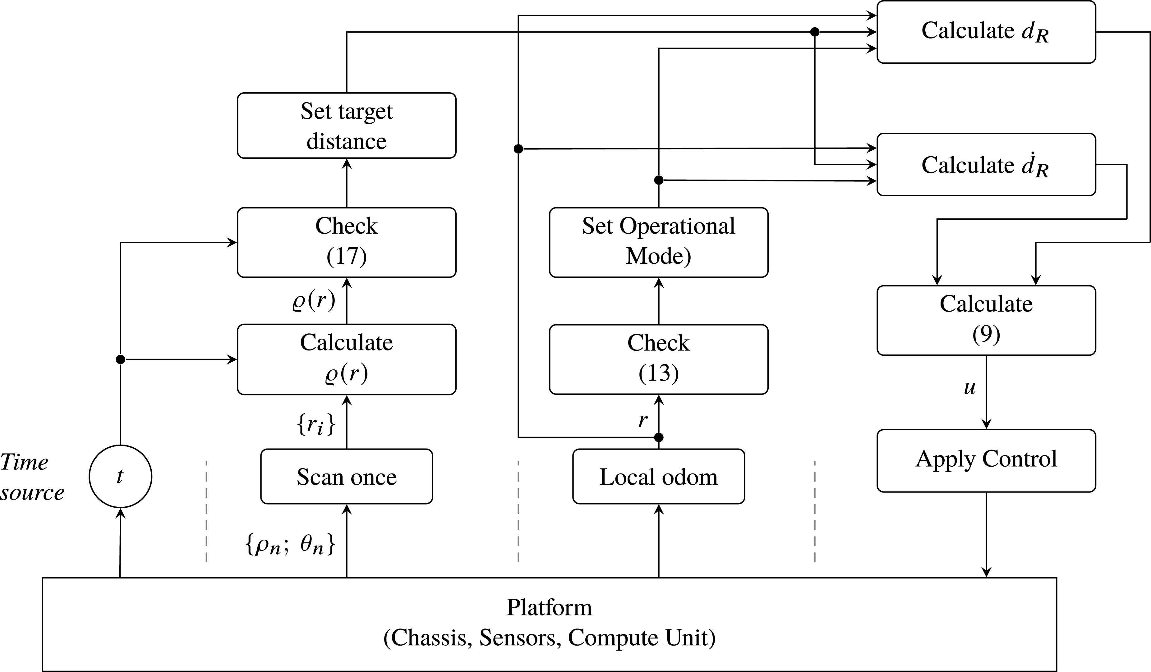


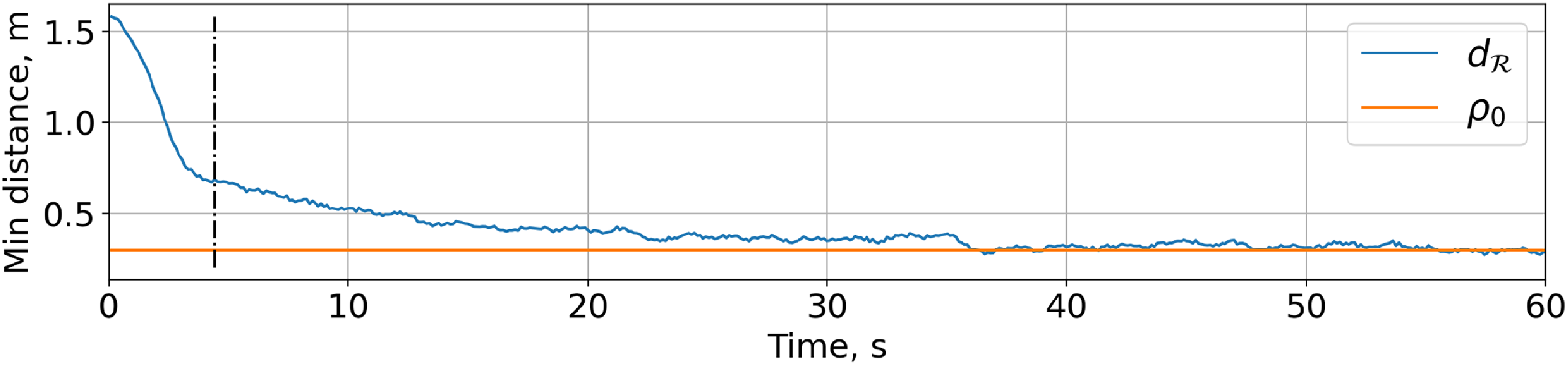
 d
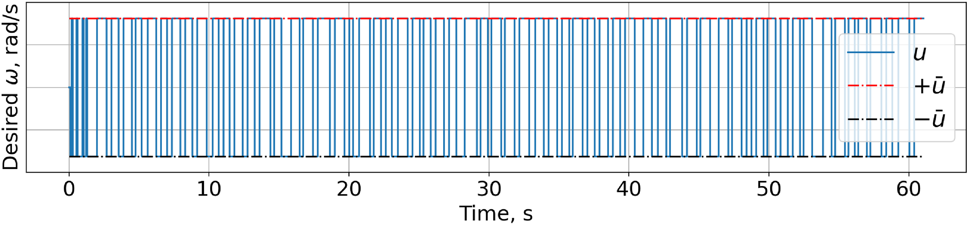
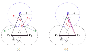
 A


