Theoretical collision model of elongated particles in turbulence

Haoran Luo; Jianda Huang; Lihao Zhao

doi:10.1017/jfm.2026.11240

Theoretical collision model of elongated particles in turbulence

Published online by Cambridge University Press: 05 March 2026

and

Haoran Luo: Affiliation:
Xingjian College, Tsinghua University, Beijing 100084, PR China
Jianda Huang: Affiliation:
AML, Department of Engineering Mechanics, Tsinghua University, Beijing 100084, PR China
Lihao Zhao*: Affiliation:
AML, Department of Engineering Mechanics, Tsinghua University, Beijing 100084, PR ChinaState Key Laboratory of Advanced Space Propulsion, Tsinghua University, 100084, Beijing
*: Corresponding author: Lihao Zhao, zhaolihao@mail.tsinghua.edu.cn

Article contents

Abstract
Introduction
Numerical methods
Results
Conclusions and outlooks
Funding
Declaration of interests
References

Rights & Permissions

Abstract

The collisions between elongated particles in turbulence play an important role in various natural and industrial processes. In this study, we establish a theoretical model to estimate the collision kernels of monodisperse elongated passive particles in homogeneous isotropic turbulence. The model is composed of two terms: the collision kernel with fixed relative angles and the angular-volumetric number density of neighbouring pairs, where we first derive under the Gaussian hypothesis of the fluid velocity gradients and then incorporate a non-Gaussianity factor into the formulations. The collision kernels obtained by the present model are in a good agreement with that of direct numerical simulations. Moreover, our model provides insights into the mechanism of the relative alignment between nearby particle pairs and the chain formation in turbulence, from the perspective of particle collisions.

JFM classification

Turbulent Flows: Isotropic turbulence Biological Fluid Dynamics: Collective behaviour

Information

Type: JFM Papers
Information: Journal of Fluid Mechanics , Volume 1030 , 10 March 2026, A38
DOI: https://doi.org/10.1017/jfm.2026.11240 [Opens in a new window]
Copyright: © The Author(s), 2026. Published by Cambridge University Press

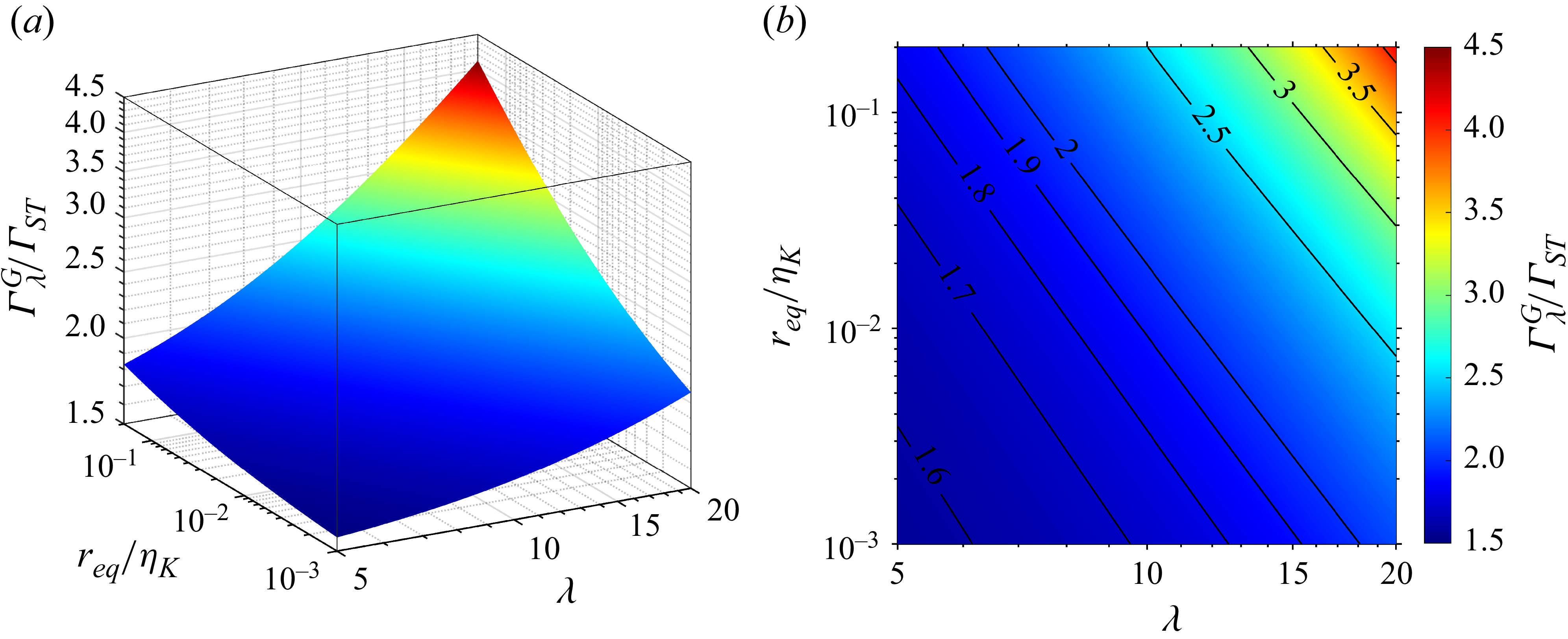
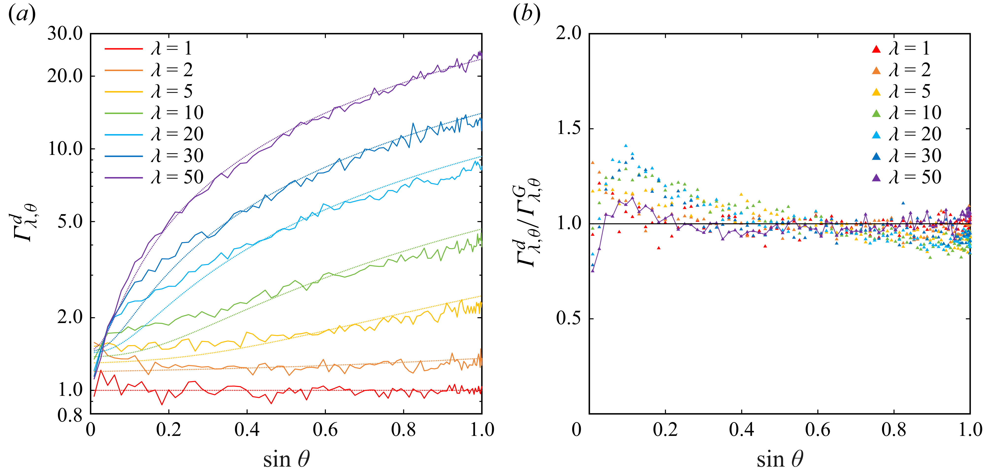
1. Introduction

Suspensions of non-spherical particles in turbulence are commonly observed in natural and industrial processes (Voth & Soldati Reference Voth and Soldati2017; Brandt & Coletti Reference Brandt and Coletti2022), such as phytoplankton in oceanic flows (Guasto, Rusconi & Stocker Reference Guasto, Rusconi and Stocker2012; Durham et al. Reference Durham, Climent, Barry, Lillo, Boffetta, Cencini and Stocker2013; Sengupta, Carrara & Stocker Reference Sengupta, Carrara and Stocker2017), ice crystals in turbulent clouds (Pruppacher & Klett Reference Pruppacher and Klett2010; Jucha et al. Reference Jucha, Naso, Lévêque and Pumir2018; Sheikh et al. Reference Sheikh, Gustavsson, Lévêque, Mehlig, Pumir and Naso2022) and pulp fibres in papermaking (Lundell, Söderberg & Alfredsson Reference Lundell, Söderberg and Alfredsson2011). These suspended particles collide with each other and merge into larger aggregates or split into fragments, which triggers the formation of marine snow (Thornton Reference Thornton2002) and the generation of secondary atmospheric ice particles (Vardiman Reference Vardiman1978; Lawson et al. Reference Lawson, Bruintjes, Woods and Gurganus2022). Therefore, it is necessary to understand the collision behaviour of non-spherical particles in turbulence, despite their complex geometry.

As a simplified case, collisions of spherical particles in turbulence have been widely studied (Sundaram & Collins Reference Sundaram and Collins1997; Wang et al. Reference Wang, Wexler and Zhou1998a , Reference Wang, Wexler and Zhoub ; Mei & Hu Reference Mei and Hu1999; Meyer & Deglon Reference Meyer and Deglon2011). Specifically, in a multi-particle system, the collision rate of dispersed particles is quantified by the collision kernel defined as

(1.1)

\begin{align} \varGamma ^{{d}}=\frac {2\dot {n}_{\textit{coll}}}{n_{\textit{part}}^2}, \end{align}

where $\dot {n}_{\textit{coll}}$ denotes the number of collisions that occur per unit volume and per unit time and $n_{\textit{part}}$ denotes the number of particles per unit volume (Wang et al. Reference Wang, Wexler and Zhou1998a ). The collision kernel defined in (1.1) is referred to as the dynamic collision kernel (denoted by the superscript ‘d’ in this paper). One needs to detect and count collision events in the multi-particle system to obtain $\varGamma ^{{d}}$ (Wang et al. Reference Wang, Ayala, Kasprzak and Grabowski2005), either by conducting experiments or by Monte Carlo simulations.

Alternatively, the collision kernel can also be described in an equivalent kinematic manner as the average inward flux of particles across the surface of a contact region per unit time (Saffman & Turner Reference Saffman and Turner1956; Wang, Wexler & Zhou Reference Wang, Wexler and Zhou2000). Here, the concept of contact region is applied to recognise the finite range in the particle frame where two particles can interact, thus collisions happen when the centre of one particle moves into another’s contact region. For spherical particles, the contact region is a concentric sphere with a radius equal to the particle diameter (Saffman & Turner Reference Saffman and Turner1956; Gerritsen & Strickler Reference Gerritsen and Strickler1977; Evans Reference Evans1989; Lewis & Pedley Reference Lewis and Pedley2000; Wang et al. Reference Wang, Wexler and Zhou2000). The kinematic collision kernel of spherical tracers in homogeneous isotropic turbulence (HIT) was first estimated by Saffman & Turner (Reference Saffman and Turner1956), using the total inward flux of relative fluid velocity on the spherical surface of the contact region:

(1.2)

\begin{align} \varGamma _{\textit{ST}}(r) = 4\pi R^2 \big\langle |\Delta u_r^-(R)|\big\rangle = (2r)^3\sqrt {\frac {8\pi \varepsilon }{15\nu }}. \end{align}

Here, $\nu$ and $\varepsilon$ are the fluid kinematic viscosity and the mean energy dissipation rate of turbulence, respectively; $r$ is the particle radius and $\Delta u_r(R)$ is the radial relative velocity (RRV) of the fluid, with a separation distance $R=2r$ . Additionally, $\langle |\Delta u_r^-(R)|\rangle =\langle -\min \{\Delta u_r(R), 0\}\rangle$ represents the value of the negative-part expectation of RRV, equal to $\langle |\Delta u_r^+(R)|\rangle =\langle \max \{\Delta u_r(R), 0\}\rangle$ since the inward and outward fluxes balance on the spherical surface by incompressibility. To derive (1.2), Saffman & Turner (Reference Saffman and Turner1956) assumed that (i) $r\lt \eta _{{K}}=(\nu ^3/\varepsilon )^{1/4}$ (the Kolmogorov length scale of turbulence), (ii) the flow is locally isotropic and (iii) the probability distributions of the velocity gradients $A_{\textit{ij}}=\partial u_i/\partial x_j$ are Gaussian, which lead to

(1.3)

\begin{align} \big\langle |\Delta u_r^-(R)| \big\rangle =R\big\langle |A_{11}^-| \big\rangle =R\frac {1}{\sqrt {2\pi }}\sqrt {\frac {\varepsilon }{15\nu }}. \end{align}

Subsequent studies have incorporated the radial distribution function $g(R)$ into the collision kernel formulation to account for the non-uniform concentration of spherical particles with inertia (Sundaram & Collins Reference Sundaram and Collins1997; Reade & Collins Reference Reade and Collins2000; Wang et al. Reference Wang, Wexler and Zhou2000; Franklin et al. Reference Franklin, Vaillancourt, Yau and Bartello2005), which reduces to $g(R)=1$ for passive inertialess particles with random seeding considered in this paper. For simplicity and clarity, all the collision kernels without the superscript ‘d’ refer to the kinematic kernels, distinguished from the dynamic ones.

However, very few theoretical advancements have been made for the collision kernel of non-spherical particles in previous studies. Siewert, Kunnen & Schröder (Reference Siewert, Kunnen and Schröder2014) considered gravitational settling ellipsoids with uncorrelated random orientations in weak turbulence, in which the kinematic kernel is approximately integrated on the surface of an equal-volume spherical region, while Gavze & Khain (Reference Gavze and Khain2022) introduced a collecting area between settling pairs by geometric analyses, without considering the influence of turbulent flow. Słomka & Stocker (Reference Słomka and Stocker2020) and Jiang, Xu & Zhao (Reference Jiang, Xu and Zhao2024) also studied the collision kernels of rods and spheroids with an offset mass centre, respectively, when settling in a quiescent fluid with random or fixed pitch angles. In addition to the aforementioned theoretical studies, recently, direct numerical simulation (DNS) has been widely adopted for simulating spheroidal particles in turbulence and computing the dynamic kernel by numerical data directly, which is however computationally expensive (Arguedas-Leiva et al. Reference Arguedas-Leiva, Słomka, Lalescu, Stocker and Wilczek2022; Grujić et al. Reference Grujić, Bhatnagar, Sardina and Brandt2024). Therefore, a theoretical model is needed for accurate and efficient predictions of the collision kernel for non-spherical particles in turbulence.

In this paper, we focus on the particles with representative elongated geometry and establish a theoretical collision model for monodisperse elongated passive particles in HIT. We adopt theoretical analyses and statistics of DNS to construct our model, which performs well in predicting the collision kernels of particles in a wide range of particle size, aspect ratio and Reynolds number. Based on our model, we further explore the intriguing physics of the relative alignment between colliding particle pairs.

2. Numerical methods

Apart from theoretical derivations, we obtain statistics from DNS for the construction, analyses and verification of our collision model. In DNS, we adopt a one-way coupling Eulerian–Lagrangian method to simulate elongated passive particles in HIT. The dynamics of the fluid phase is solved in a Eulerian frame and each particle is tracked along the Lagrangian trajectory using local flow information at the centre of the particle (Qiu et al. Reference Qiu, Cui, Climent and Zhao2022a , Reference Qiu, Mousavi, Zhao and Gustavssonb , Reference Qiu, Cui, Climent and Zhao2024).

2.1. Fluid phase

The HIT is directly simulated by solving the incompressible Navier–Stokes equations

(2.1)

\begin{align} \frac {\partial \boldsymbol{u}}{\partial t}+\boldsymbol{u}\boldsymbol{\cdot }\boldsymbol{\nabla }\boldsymbol{u}=-\frac {\boldsymbol{\nabla }\!p_{\kern-2pt {f}}}{\rho _{\kern-1.5pt{f}}}+\nu {\nabla} ^2\boldsymbol{u}+\boldsymbol{f}, \\[-28pt] \nonumber \end{align}

(2.2)

\begin{align} \boldsymbol{\nabla }\boldsymbol{\cdot }\boldsymbol{u}=0, \\[0pt] \nonumber \end{align}

where $\boldsymbol{u}$ is the fluid velocity, while $p_{\kern-2pt {f}}$ , $\rho _{\kern-1.5pt{f}}$ and $\nu$ are the pressure, density and kinematic viscosity of the fluid, respectively. To sustain the turbulence, an external force $\boldsymbol{f}$ is applied to the large scales and injects energy, which balances the rate of viscous dissipation at the Kolmogorov length scale $\eta _{{K}}$ (Machiels Reference Machiels1997).

Equations (2.1) and (2.2) are solved in the Eulerian frame using a pseudospectral method (Pope Reference Pope2000). For time integration, we use an explicit second-order Adams–Bashforth scheme (Rogallo Reference Rogallo1981). The size of the cubic computational domain is $(2\pi )^3$ and three-dimensional periodic boundary conditions are applied to each wall of the domain.

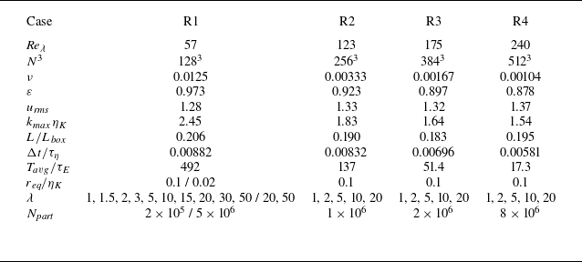
In DNS, we simulate four cases with different Taylor–Reynolds number $ \textit{Re}_{\lambda } = u_{\textit{rms}}^2 \sqrt {15/\nu \varepsilon }$ (where $u_{\textit{rms}}$ is the root-mean-square fluid velocity), referred to as ‘R1–R4’ (see table 1 for the parameters). HIT with $ \textit{Re}_{\lambda }=57, 123, 175$ and $240$ is resolved by $128^3$ , $256^3$ , $384^3$ and $512^3$ grid points, respectively. In each case, $k_{\textit{max}}\eta _{{K}}\gt 1.5$ , ensuring that the maximum resolved wavenumber is adequately greater than the Kolmogorov wavenumber. The time step $\Delta t$ is much smaller than the Kolmogorov time scale $\tau _{\eta }=\sqrt {\nu /\varepsilon }$ to resolve small-scale flow dynamics, and to precisely capture particle motions and collision events.

Table 1.

Cases and corresponding parameters of the fluid and particles in DNS. Here, $L$ is the integral length scale of turbulence (characterised by the domain size $L_{{box}}=2\pi$ ), $\tau _{{E}} = L/u_{\textit{rms}}$ is the large-eddy turnover time and other parameters are defined in the main text. All values are dimensionalised or in code units.

2.2. Particle phase

In the present collision model, the geometry of elongated particles is modelled as a cylinders with hemispherical caps (Arguedas-Leiva et al. Reference Arguedas-Leiva, Słomka, Lalescu, Stocker and Wilczek2022). Given the radius $a$ and aspect ratio $\lambda$ , the width and length of particles are $2a$ and $2\lambda a$ , respectively. An equivalent radius $r_{\textit{eq}}=a\lambda ^{1/3}$ is proposed to quantify the characteristic size of particles and is fixed when discussing the elongation effect.

Although the particle geometry is complex for the point-particle approach, previous studies by the slender-body theory, simulations and experiments have demonstrated that the rotation rate of small rigid rod-like particles in HIT coincides well with that of inertialess ellipsoids (Shin & Koch Reference Shin and Koch2005; Parsa et al. Reference Parsa, Guasto, Kishore, Ouellette, Gollub and Voth2011, Reference Parsa, Calzavarini, Toschi and Voth2012; Ravnik & Marchioli Reference Ravnik and Marchioli2018). Hence, the translation and rotation of our elongated passive particles are governed by

(2.3)

\begin{align} \frac {\mathrm{d}\boldsymbol{x}}{\mathrm{d}t} = \boldsymbol{u}(\boldsymbol{x}), \\[-28pt] \nonumber \end{align}

(2.4)

\begin{align} \frac {\mathrm{d}\boldsymbol{p}}{\mathrm{d}t} = \frac {1}{2} \boldsymbol{\varOmega }(\boldsymbol{x}) \times \boldsymbol{p} + \varLambda [ \unicode{x1D644}-\boldsymbol{p}\boldsymbol{p}] \boldsymbol{\cdot }\unicode{x1D64E}(\boldsymbol{x}) \boldsymbol{\cdot }\boldsymbol{p}, \\[-2pt] \nonumber \end{align}

where the shape factor is

(2.5)

\begin{align} \varLambda = \frac {\lambda ^2-1}{\lambda ^2+1}, \end{align}

which relies on the aspect ratio $\lambda$ (Jeffery Reference Jeffery1922). Here, $\boldsymbol{x}$ and $\boldsymbol{p}$ are the position and orientation of particles, respectively. Additionally, $\boldsymbol{u}(\boldsymbol{x})$ , $\boldsymbol{\varOmega }(\boldsymbol{x})$ and $ \unicode{x1D64E}(\boldsymbol{x})$ stand for the velocity, vorticity, and strain rate of the local fluid, respectively, all interpolated by a second-order Lagrangian method using fluid information at the Eulerian grid points.

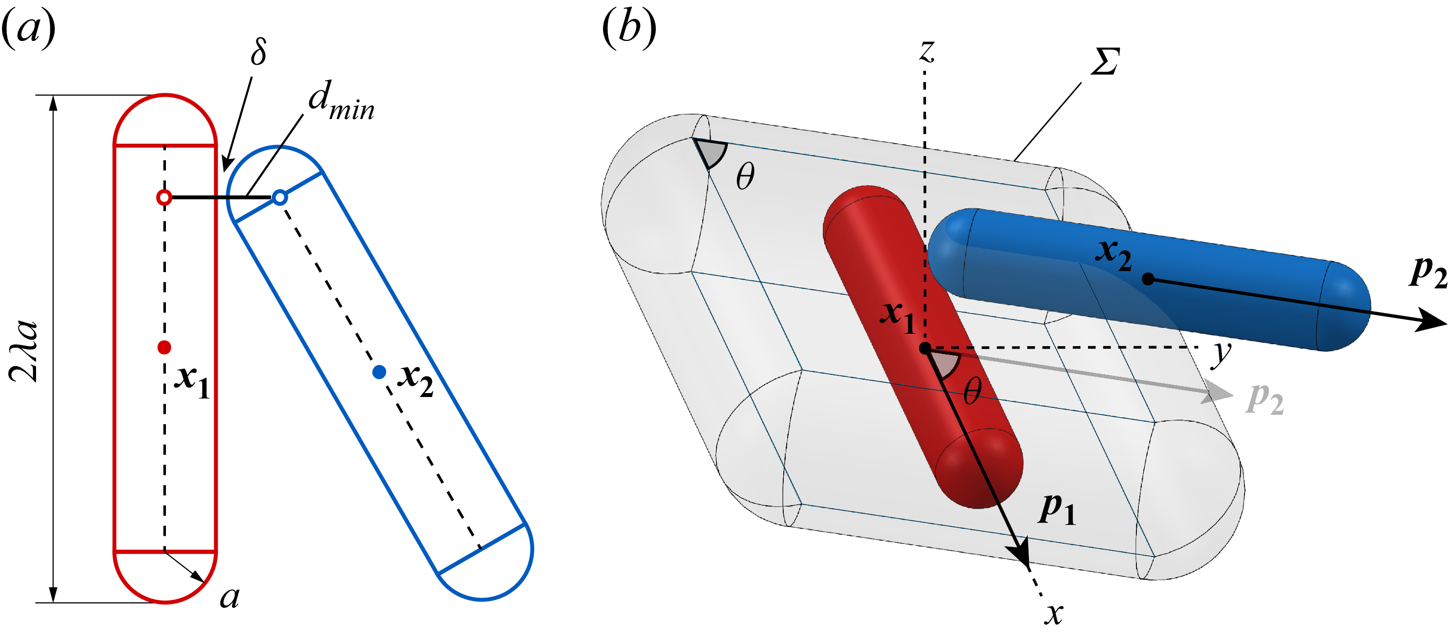
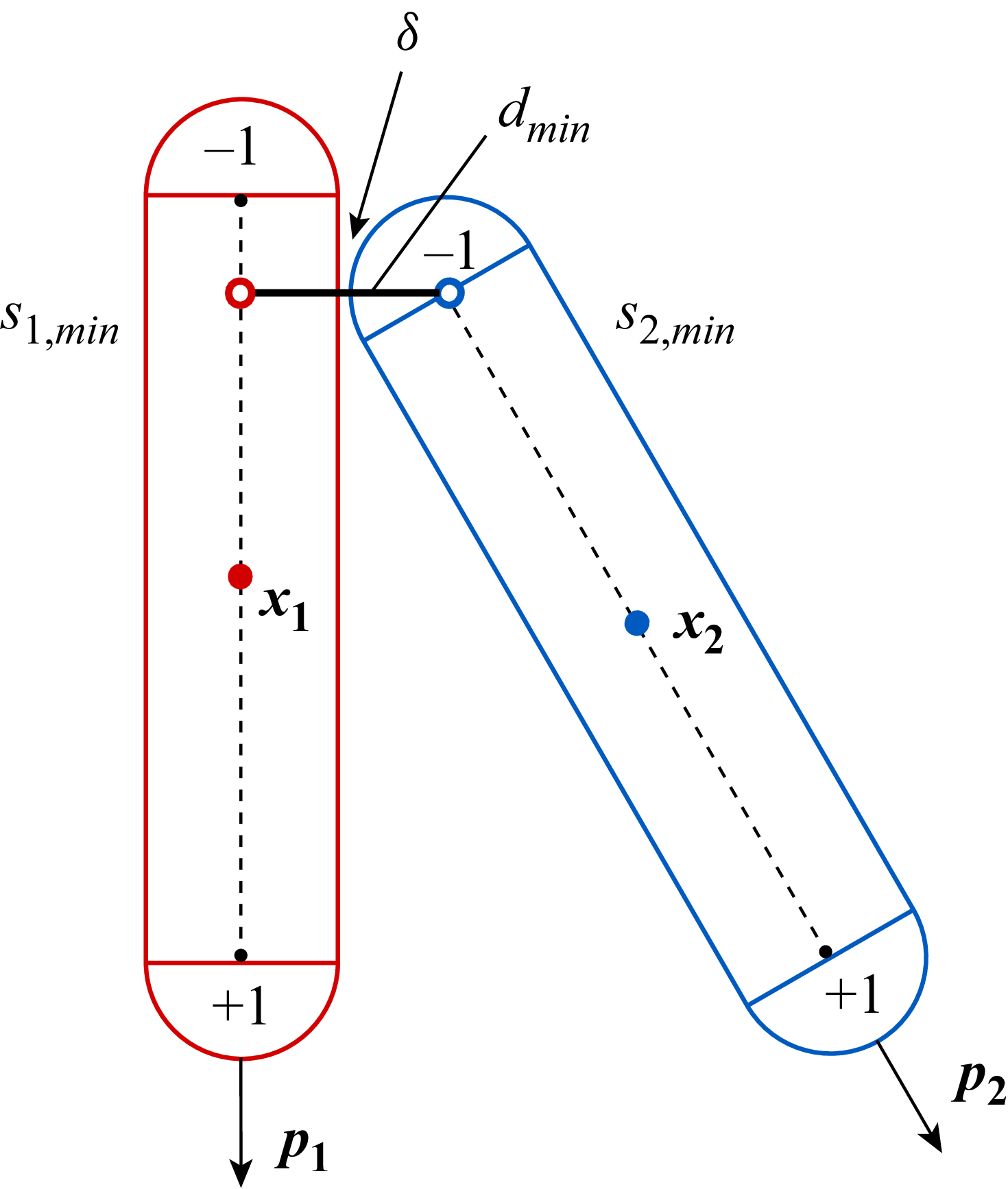
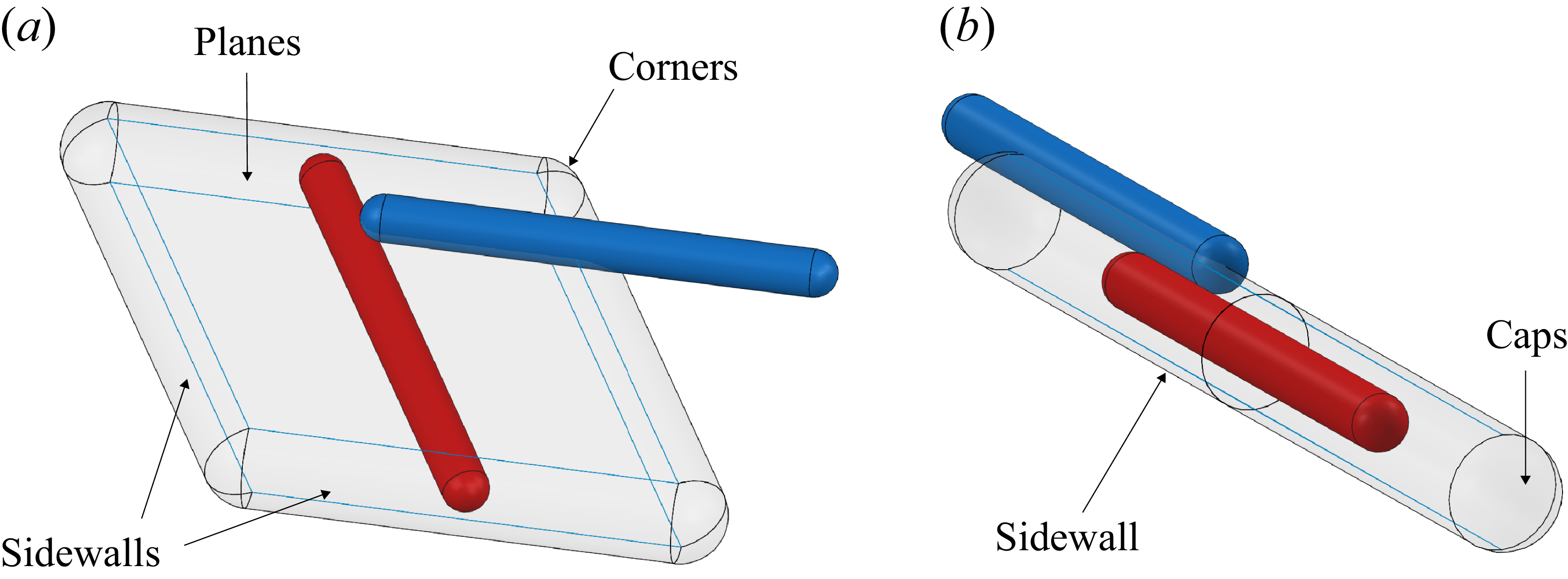
The collision detection of elongated particles is performed by calculating the minimal distance $d_{\textit{min}}$ between the two symmetry axes of a pair of particles, and comparing the interparticle distance $\delta =d_{\textit{min}}-2a$ with zero (see figure 1 a for sketch and Appendix A for detailed algorithm). Meanwhile, the ghost collision assumption is adopted, so that particles do not affect each other during the collision process. This idealised assumption is appropriate and widely applied for dilute suspensions with low collision frequency (Zhou, Wexler & Wang Reference Zhou, Wexler and Wang2001; Bec et al. Reference Bec, Celani, Cencini and Musacchio2005, Reference Bec, Biferale, Cencini, Lanotte and Toschi2010; Wang et al. Reference Wang, Rosa, Gao, He and Jin2009; Arguedas-Leiva et al. Reference Arguedas-Leiva, Słomka, Lalescu, Stocker and Wilczek2022; Grujić et al. Reference Grujić, Bhatnagar, Sardina and Brandt2024; Jiang et al. Reference Jiang, Xu and Zhao2024), and is naturally compatible with both kinematic and dynamic formulations of the collision kernel (Wang et al. Reference Wang, Wexler and Zhou1998a ). Near-contact hydrodynamic interactions and post-contact outcomes (e.g. lubrication, adhesion, coalescence and rebound) are commonly absorbed into a separate efficiency factor by more realistic numerical simulations or experiments (Bordás et al. Reference Bordás, Hagemeier, Wunderlich and Thévenin2011, Reference Bordás, Roloff, Thévenin and Shaw2013; Chen, Yau & Bartello Reference Chen, Yau and Bartello2018; Ababaei et al. Reference Ababaei, Rosa, Pozorski and Wang2021), and are therefore out of the present scope to isolate the effects of turbulence and particle shape on the collision dynamics.

After the turbulence is fully developed, elongated passive particles are released with random initial positions and orientations. For each particle parameter configuration, elongated particles with a total amount $N_{\textit{part}}$ are simulated over $10\tau _{\eta }$ until statistically stationary, and then the statistics are averaged over a subsequent $T_{{avg}}$ . Detailed particle configurations are also listed in table 1.

3. Results

Despite the evolution of particle orientations during the collision process, we focus on the collision instant, and thus first explore the theoretical collision kernel with fixed relative angles defined at collisions, in § 3.1. We then compute the probability of particle pairs approaching at a given relative angle by DNS in § 3.2, thereby closing and validating our model in § 3.3. Moreover, we demonstrate the insights of our model into the physics of preferential alignment in § 3.4 and the statistics of collision states in § 3.5.

3.1. Collision kernel with fixed relative angles

To theoretically derive the collision kernel, we reconstruct the contact region for elongated particles in our model, which is technically obtained by fixing one particle (particle 1) at the origin and tracing the centre of another particle (particle 2) while moving along the surface of particle 1, with their orientations fixed. We define $\theta \in [0,\pi /2]$ as the relative angle between the orientations of a pair of particles to characterise their relative alignment. By setting the orientations $\boldsymbol{p}_1 = [1,0,0]^{\prime }$ and $\boldsymbol{p}_2 = [\cos \theta ,\sin \theta ,0]^{\prime }$ for a pair of particles at the collision instant, the geometry of the contact region is correspondingly demonstrated in figure 1(b). The contact region is composed of a quadrangular prism, four hemicylinders and four portions of a sphere. Here, $\varSigma$ represents the surface of the contact region, with its normal vector denoted by $\boldsymbol{n}_{\varSigma }$ .

Figure 1.

(a) Sketch of an elongated particle pair and the collision detection method. (b) The contact region (grey) with its surface $\varSigma$ , when particle 2 (blue) approaches particle 1 (red) with a fixed relative angle $\theta$ . The contact region is a quadrangular prism with hemicylindrical sidewalls and spherical corners.

3.1.1. General theoretical formulation

In contrast to spherical particles, the rotational dynamics of elongated particles are important in their collision process. Specifically, the collision rates are dependent on the relative velocity between the two colliding points on the surface of a particle pair. Here, we consider a subset of particles, in which all collisions occur with a fixed relative angle $\theta$ . As a result, the collision kernel in this subset is theoretically expressed by integrating the average inward flux of the relative velocity between the colliding points, performed on the surface of the contact region (see the verification in Appendix E):

(3.1)

where $\boldsymbol{v}_{\!p1}(\boldsymbol{x}_{\textit{coll}})$ and $\boldsymbol{v}_{\!p2}(\boldsymbol{x}_{\textit{coll}})$ are the velocity of the two colliding points, respectively, and (3.1) depends on the negative-part expectation of surface-normal relative velocity, i.e. $\langle | [ ( \boldsymbol{v}_{\!p2}(\boldsymbol{x}_{\textit{coll}})-\boldsymbol{v}_{\!p1}(\boldsymbol{x}_{\textit{coll}}) ) \boldsymbol{\cdot }\boldsymbol{n}_{\varSigma } ]^- | \rangle$ . In the frame of particle 1, $\boldsymbol{x}_2$ (the centre of particle 2) is on $\varSigma$ , while the relative velocity between the colliding points is

(3.2)

\begin{align} \boldsymbol{v}_{\!p2}(\boldsymbol{x}_{\textit{coll}})-\boldsymbol{v}_{\!p1}(\boldsymbol{x}_{\textit{coll}}) = \boldsymbol{v}_2^{(1)}+\boldsymbol{\omega }_2^{(1)} \times (\boldsymbol{x}_{\textit{coll}}-\boldsymbol{x}_2), \end{align}

where $\boldsymbol{v}_2^{(1)}$ and $\boldsymbol{\omega }_2^{(1)}$ are the velocity and angular velocity of particle 2 in the frame of particle 1, respectively. We use the equivalent form of (2.4), which governs the angular velocity of passive ellipsoidal particles in the Eulerian frame:

(3.3)

\begin{align} \boldsymbol{\omega }(\boldsymbol{x},\boldsymbol{p}) = \frac {1}{2}\boldsymbol{\varOmega }(\boldsymbol{x})+\varLambda \boldsymbol{p}\times \unicode{x1D64E}(\boldsymbol{x})\boldsymbol{\cdot }\boldsymbol{p}. \end{align}

According to Helmholtz velocity decomposition and the governing equations of particles, we transform the relative velocity and angular velocity of local fluid into the frame of particle 1 by setting $\boldsymbol{x}_1 = \boldsymbol{0}$ , $\boldsymbol{p}_1 = [1,0,0]^{\prime }$ and $\boldsymbol{p}_2 = [\cos \theta ,\sin \theta ,0]^{\prime }$ . As a result,

(3.4)

\begin{align} \boldsymbol{v}_2^{(1)}&=\boldsymbol{u}(\boldsymbol{x}_2)-\boldsymbol{u}(\boldsymbol{0})-\boldsymbol{\omega }(\boldsymbol{0},\boldsymbol{p}_1)\times \boldsymbol{x}_2 \nonumber \\[4pt]&\approx \left (\frac {1}{2}\boldsymbol{\varOmega }\times \boldsymbol{x}_2+\boldsymbol{x}_2\boldsymbol{\cdot }\unicode{x1D64E}\right ) - \left (\frac {1}{2}\boldsymbol{\varOmega }+\varLambda \boldsymbol{p}_1\times \unicode{x1D64E}\boldsymbol{\cdot }\boldsymbol{p}_1\right )\times \boldsymbol{x}_2 \nonumber \\[4pt]&=\boldsymbol{x}_2\boldsymbol{\cdot }\unicode{x1D64E}-\varLambda (\boldsymbol{p}_1\times \unicode{x1D64E}\boldsymbol{\cdot }\boldsymbol{p}_1)\times \boldsymbol{x}_2 \nonumber \\[4pt]&=\begin{bmatrix} {S}_{11} & (1+\varLambda ){S}_{21} & (1+\varLambda ){S}_{31} \\[4pt] (1-\varLambda ){S}_{12} & {S}_{22} & {S}_{32} \\[4pt] (1-\varLambda ){S}_{13} & {S}_{23} & {S}_{33} \\ \end{bmatrix} \boldsymbol{x}_2, \\[-28pt] \nonumber \end{align}

(3.5)

\begin{align} \boldsymbol{\omega }_2^{(1)} &= \boldsymbol{\omega }(\boldsymbol{x}_2,\boldsymbol{p}_2)-\boldsymbol{\omega }(\boldsymbol{0},\boldsymbol{p}_1) \nonumber\\[4pt]&\approx \boldsymbol{\omega }(\boldsymbol{0},\boldsymbol{p}_2)-\boldsymbol{\omega }(\boldsymbol{0},\boldsymbol{p}_1) \nonumber\\[4pt]&= \varLambda (\boldsymbol{p}_2\times \unicode{x1D64E}\boldsymbol{\cdot }\boldsymbol{p}_2 - \boldsymbol{p}_1\times \unicode{x1D64E}\boldsymbol{\cdot }\boldsymbol{p}_1) \nonumber\\[4pt]&= \varLambda \sin \theta \begin{bmatrix} {S}_{13}\cos \theta +{S}_{23}\sin \theta \\[4pt] {S}_{13}\sin \theta -{S}_{23}\cos \theta \\[4pt] ({S}_{22}-{S}_{11})\cos \theta -2{S}_{12}\sin \theta \\ \end{bmatrix} \!. \\[0pt] \nonumber \end{align}

Here, $\boldsymbol{\varOmega }$ and $ \unicode{x1D64E}$ are both extracted at the centre of particle 1 in the Eulerian frame, and ${S}_{\textit{ij}} = (\partial u_i/\partial x_j+\partial u_{\kern-1.5pt j}/\partial x_i)/2$ is the component of the strain-rate tensor $ \unicode{x1D64E}$ . Introducing the velocity gradient tensor (VGT) $ \unicode{x1D63C}=\boldsymbol{\nabla }\boldsymbol{u}$ , the surface-normal relative velocity is expressed as a linear combination of $A_{\textit{ij}}$ :

(3.6)

\begin{align} ( \boldsymbol{v}_{\!p2}(\boldsymbol{x}_{\textit{coll}})-\boldsymbol{v}_{\!p1}(\boldsymbol{x}_{\textit{coll}}) ) \boldsymbol{\cdot }\boldsymbol{n}_{\varSigma } = \unicode{x1D63E}: \unicode{x1D63C} = C_{\textit{ij}}A_{\textit{ij}}, \end{align}

which is a scalar. Apart from the relative angle $\theta$ , the coefficients of this linear combination, $C_{\textit{ij}}$ , also depend on the centre position $\boldsymbol{x}_2$ of particle 2 and the colliding point $\boldsymbol{x}_{\textit{coll}}$ . Accordingly, the collision kernel with fixed relative angles is reformulated as

(3.7)

Here, we first derive the standard deviation of $ \unicode{x1D63E}: \unicode{x1D63C}$ . In incompressible HIT, the second-order statistics of VGT components are given by

(3.8)

\begin{align} \left \langle A_{\textit{ij}}(\boldsymbol{x}) A_{kl}(\boldsymbol{x}) \right \rangle = \frac {\varepsilon }{30\nu }(4\delta _{ik}\delta _{jl}-\delta _{il}\delta _{jk}-\delta _{\textit{ij}}\delta _{kl}), \end{align}

where $\delta _{\textit{ij}}$ denotes the Kronecker delta. Specifically, the variances and covariances of longitudinal and transverse VGT components are

(3.9)

\begin{align} \big \langle A_{11}^2 \big \rangle = \sigma ^2,\quad \big \langle A_{12}^2\big \rangle = 2\sigma ^2,\quad\left \langle A_{11}A_{22}\right \rangle = \left \langle A_{12}A_{21}\right \rangle = -\frac {\sigma ^2}{2}, \end{align}

where $\sigma = \sqrt {\varepsilon /15\nu }$ . Therefore, the standard deviation of $ \unicode{x1D63E}: \unicode{x1D63C}$ is

(3.10)

\begin{align} \sigma _{ \unicode{x1D63E}: \unicode{x1D63C}} = \sigma \sqrt {2\Vert \unicode{x1D63E}\Vert _F^2 - \frac {1}{2}\mathrm{tr}( \unicode{x1D63E}^2) - \frac {1}{2}(\mathrm{tr} \unicode{x1D63E})^2} = \sigma \sqrt {2C_{\textit{ij}}C_{\textit{ij}} - \frac {1}{2}C_{\textit{ij}}C_{\textit{ji}} - \frac {1}{2}(C_{\textit{ii}})^2}. \end{align}

Figure 2.

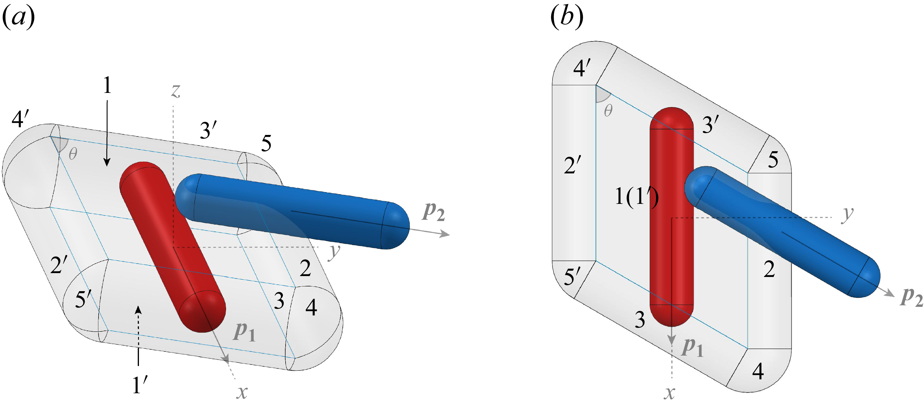
(a) Zone divisions on the surface of the contact region, with the top view in panel (b). The plotted case corresponds to $\lambda =5$ and $\theta =\pi /3$ .

Further considering the surface integration in (3.7), we devide the surface of the contact region into five pairs of zones, as shown in figure 2: the upper and lower planes (zones $1\unicode{x2013}1'$ ), the left–right and front–back hemicylindrical sidewalls (zones $2\unicode{x2013}2'$ and $3\unicode{x2013}3'$ ), and the major and minor spherical corners (zones $4\unicode{x2013}4'$ and $5\unicode{x2013}5'$ ). 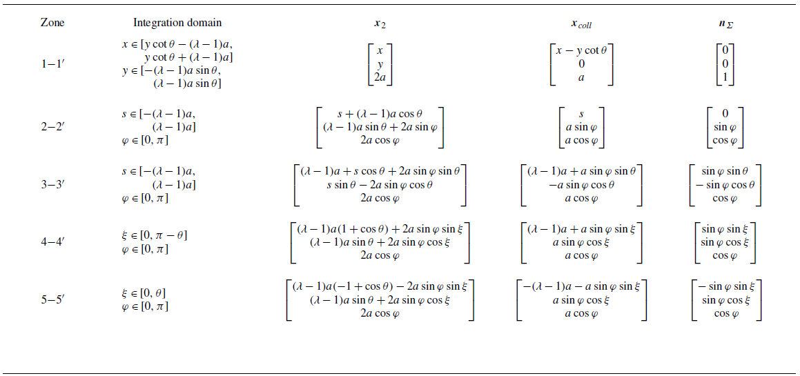Numerical integrations are performed separately in all these zones, with the integration domains and key parameters ( $\boldsymbol{x}_2$ , $\boldsymbol{x}_{\textit{coll}}$ and $\boldsymbol{n}_{\varSigma }$ ) listed in table 2. The coefficient tensor $ \unicode{x1D63E}$ in each zone can therefore be calculated separately.

Table 2.

Numerical integration domains and parameters in different zones of the contact region. Here, $x$ , $y$ , $s$ and $\xi$ , $\varphi$ stand for lengthwise and angular coordinates, respectively.

Take zone 1 (the upper plane) as an example. For each point $[x,y,2a]^{\prime }$ in zone 1,

(3.11)

\begin{align} ( \boldsymbol{v}_{\!p2}(\boldsymbol{x}_{\textit{coll}})& -\boldsymbol{v}_{\!p1}(\boldsymbol{x}_{\textit{coll}}) ) \boldsymbol{\cdot }\boldsymbol{n}_{\varSigma } = \left ( \begin{bmatrix} {S}_{11} & (1+\varLambda ){S}_{21} & (1+\varLambda ){S}_{31} \\[4pt] (1-\varLambda ){S}_{12} & {S}_{22} & {S}_{32} \\[4pt] (1-\varLambda ){S}_{13} & {S}_{23} & {S}_{33} \\ \end{bmatrix} \begin{bmatrix} x \\ y \\ 2a \\ \end{bmatrix} \right . \nonumber \\&\left . \quad + \varLambda \sin \theta \begin{bmatrix} {S}_{13}\cos \theta +{S}_{23}\sin \theta \\[4pt] {S}_{13}\sin \theta -{S}_{23}\cos \theta \\[4pt] ({S}_{22}-{S}_{11})\cos \theta -2{S}_{12}\sin \theta \\ \end{bmatrix} \times \begin{bmatrix} -y\cot \theta \\ -y \\ -a \\ \end{bmatrix} \right ) \boldsymbol{\cdot }\begin{bmatrix} 0 \\ 0 \\ 1 \\ \end{bmatrix} \nonumber \\&= (1-\varLambda ) x {S}_{13}+(1-\varLambda ) y {S}_{23}+2a {S}_{33} \nonumber \\&= \frac {1-\varLambda }{2}x\left (A_{13}+A_{31}\right ) + \frac {1-\varLambda }{2}y\left (A_{23}+A_{32}\right ) + 2a A_{33}. \end{align}

Hence, we obtain the coefficient tensor in matrix form:

(3.12)

\begin{align} \unicode{x1D63E}_{z1}= \begin{bmatrix} 0 & 0 & \frac {1-\varLambda }{2}x \\[3pt] 0 & 0 & \frac {1-\varLambda }{2}y \\[3pt] \frac {1-\varLambda }{2}x & \frac {1-\varLambda }{2}y & 2a \\ \end{bmatrix}\!, \end{align}

where the subscript ‘ $z1$ ’ denotes zone 1. According to (3.10), the standard deviation of $ \unicode{x1D63E}_{z1}: \unicode{x1D63C}$ is therefore calculated as

(3.13)

\begin{align} \sigma _{z1} = \sigma \sqrt {\frac {3(1-\varLambda )^2}{4}(x^2+y^2)+4a^2}, \end{align}

which varies with the position $(x,y)$ in zone 1. Similar derivations can be performed in other zones to obtain $\sigma _{zi}$ and $\sigma _{zi^{\prime }}\,(i=1 {-} 5)$ .

However, the standard deviations $\sigma _{zi}$ alone are insufficient to determine the negative-part expectation of surface-normal relative velocity, i.e. $\langle |( \unicode{x1D63E}: \unicode{x1D63C})^- | \rangle$ , required in (3.7). The full probability distribution functions (p.d.f.s) of $A_{\textit{ij}}$ must be incorporated for closure. The derivations in §§ 3.1.2–3.1.5 are based on the Gaussian hypothesis, while a non-Gaussian model with the DNS-based first-order statistics of $A_{\textit{ij}}$ is proposed in § 3.1.6.

3.1.2. Gaussian model

Although velocity gradients in turbulent flows are known to be non-Gaussian (Johnson & Wilczek Reference Johnson and Wilczek2024), previous theoretical works since Saffman & Turner (Reference Saffman and Turner1956) have widely adopted the Gaussian hypothesis to derive analytical expressions for the kinematic collision kernel of spherical particles in HIT, as shown in (1.1) and (1.2). The present theoretical framework also first hypothesises the joint Gaussianity of VGT components, motivated by three considerations:

(i) The Gaussian hypothesis has been shown to incur limited errors in the collision kernel of sub-Kolmogorov spheres, especially in low- $ \textit{Re}_\lambda$ HIT (Wang et al. Reference Wang, Wexler and Zhou1998b ). Extending this closure to non-spherical particles is therefore intuitive and worth exploring.
(ii) The low-order moments of $A_{\textit{ij}}$ are much less sensitive to the non-Gaussian heavy tails than higher-order moments, and the leading-order expansions of the surface-normal relative velocity in (3.6) involve only first-order moments of velocity gradients.
(iii) The Gaussian model, which by construction does not capture intermittency and does not explicitly depend on $ \textit{Re}_\lambda$ , provides a baseline for comparison and extension to high- $ \textit{Re}_\lambda$ cases, as presented in § 3.1.6 (non-Gaussian model) and § 3.3 (DNS results).

Under the present Gaussian hypothesis, the surface-normal relative velocity in zone 1, i.e. $( \boldsymbol{v}_{\!p2}(\boldsymbol{x}_{\textit{coll}})-\boldsymbol{v}_{\!p1}(\boldsymbol{x}_{\textit{coll}}) ) \boldsymbol{\cdot }\boldsymbol{n}_{\varSigma } = \unicode{x1D63E}_{z1}: \unicode{x1D63C}$ , also obeys a zero-mean Gaussian distribution with a negative-part expectation

(3.14)

\begin{align} \langle |( \unicode{x1D63E}_{z1}: \unicode{x1D63C})^- | \rangle = \frac {1}{\sqrt {2\pi }} \sigma _{z1}, \end{align}

where $\sigma _{z1}$ is the standard deviation calculated in (3.13). According to (3.7), the contribution of zone 1 to the collision kernel is

(3.15)

\begin{align} \begin{aligned} \varGamma _{z1}^{{G}} &= \int _{-(\lambda -1)a\sin \theta }^{(\lambda -1)a\sin \theta }\int _{y\cot \theta -(\lambda -1)a}^{y\cot \theta +(\lambda -1)a} \frac {1}{\sqrt {2\pi }} \sigma _{z1}(x,y)\,\mathrm{d}x\,\mathrm{d}y \\ &= \frac {\varGamma _{\textit{ST}}(r_{\textit{eq}})}{4\pi \lambda } \int _{-(\lambda -1)\sin \theta /2}^{(\lambda -1)\sin \theta /2}\int _{\hat {y}\cot \theta -(\lambda -1)/2}^{\hat {y}\cot \theta +(\lambda -1)/2} \sqrt {1+\frac {3(1-\varLambda )^2}{4}(\hat {x}^{2}+\hat {y}^{2})}\, \mathrm{d}\hat {x}\,\mathrm{d}\hat {y}, \end{aligned} \end{align}

where $\hat {x}=x/2a$ , $\hat {y}=y/2a$ and $\varGamma _{\textit{ST}}(r_{\textit{eq}}) = (2r_{\textit{eq}})^3\sqrt {8\pi \varepsilon /15\nu }$ is the collision kernel of equal-volume spherical particles. The superscript ‘G’ denotes kinematic collision kernels obtained by the Gaussian model.

Contributions of the other zones are similarly integrated. Due to the symmetry properties, there are $\varGamma _{z2}^{{G}} = \varGamma _{z3}^{{G}}$ and $\varGamma _{zi^{\prime }}^{{G}} = \varGamma _{zi}^{{G}} \, (i=1 {-} 5)$ . The collision kernel with a fixed relative angle $\theta$ is calculated by

(3.16)

\begin{align} \varGamma _{\lambda ,\theta }^{{G}} = 2\sum _{i=1}^{5} \varGamma _{zi}^{{G}} = 2\sum _{i=1}^{5} \iint _{\varSigma _{zi}}\frac {1}{\sqrt {2\pi }} \sigma _{zi}\, \mathrm{d}\varSigma . \end{align}

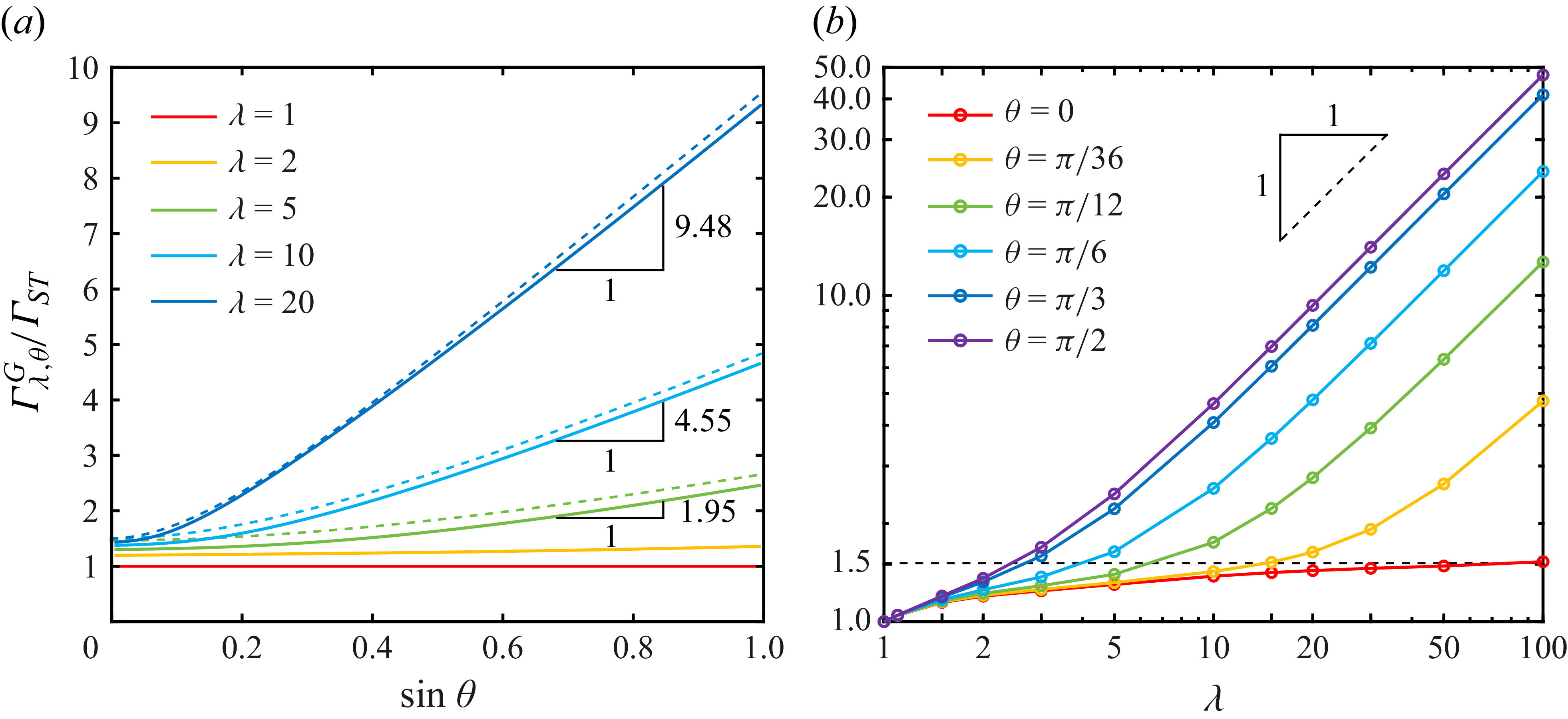
By numerical integration, we show the theoretical solutions of $\varGamma _{\lambda ,\theta }^{{G}}$ in figure 3, normalised by the equal-volume spherical kernel $\varGamma _{\textit{ST}}(r_{\textit{eq}})$ . From the asymptotes and their slopes, we find simple approximations at both the small- and large-relative-angle regimes, showing a close agreement with the theoretical solutions for highly elongated particles with $\lambda \geq 5$ :

(3.17)

\begin{align} \frac {\varGamma _{\lambda ,\theta }^{{G}}(r_{\textit{eq}},\lambda ;\theta )}{\varGamma _{\textit{ST}}(r_{\textit{eq}})} \approx \left \{ \begin{array}{ll} \,\frac {3}{2}, & \,\,\theta \rightarrow 0, \\[8pt] \frac {3}{2\pi }\lambda \sin \theta , & \,\,\frac {\pi }{6} \lesssim \theta \lt \frac {\pi }{2}, \\ \end{array} \right . \end{align}

corresponding to the almost parallel and perpendicular collisions, respectively. In §§ 3.1.3 and 3.1.4, we provide theoretical explanations for the two approximations in (3.17), which contribute to the generalisation for all relative angles in § 3.1.5.

3.1.3. Large-relative-angle regime: ${\pi }/{6} \lesssim \theta \lt {\pi }/{2}$

Here, we consider highly elongated particles colliding with almost perpendicular relative alignment, i.e. $\theta \rightarrow {\pi }/{2}$ (from figure 3 a, we find the approximation is actually precise enough when $\theta \gtrsim {\pi }/{6}$ ). As shown in figure 4(a), the contributions of the four corners to the collision kernel, i.e. $\varGamma _{z4}^{{G}}$ , $\varGamma _{z4^{\prime }}^{{G}}$ , $\varGamma _{z5}^{{G}}$ and $\varGamma _{z5^{\prime }}^{{G}}$ , are comparatively negligible due to the highly elongated particle geometry.

For the upper and lower planes (zones $1\unicode{x2013}1'$ ), the term in (3.15) satisfies

(3.18)

\begin{align} \sqrt {1+\frac {3(1-\varLambda )^2}{4}(\hat {x}^{2}+\hat {y}^{2})} \sim 1+\mathcal{O}(\lambda ^{-1}), \end{align}

where $\varLambda \sim 1-\mathcal{O}(\lambda ^{-2})$ and $\hat {x},\hat {y} \sim \mathcal{O}(\lambda )$ . Therefore,

(3.19)

\begin{align} \begin{aligned} \varGamma _{z1}^{{G}} \approx \frac {\varGamma _{\textit{ST}}}{4\pi \lambda } \int _{-(\lambda -1)\sin \theta /2}^{(\lambda -1)\sin \theta /2}\int _{\hat {y}\cot \theta -(\lambda -1)/2}^{\hat {y}\cot \theta +(\lambda -1)/2} \,\mathrm{d}\hat {x}\,\mathrm{d}\hat {y} \approx \varGamma _{\textit{ST}} \boldsymbol{\cdot }\frac {1}{4\pi } \lambda \sin \theta , \end{aligned} \end{align}

where the $\mathcal{O}(\lambda ^{-1})$ terms are ignored.

Figure 3.

Theoretical collision kernel $\varGamma _{\lambda ,\theta }^{{G}}$ of elongated particles with a fixed relative angle $\theta$ (obtained by the Gaussian model), scaled by the kernel of equal-volume spheres $\varGamma _{\textit{ST}}(r_{\textit{eq}})$ , as a function of (a) $\sin \theta$ and (b) aspect ratio $\lambda$ . The slopes of the asymptotes marked beside the vertical line segments are close to those of the two approximations in (3.17), while the coloured dashed curves correspond to the fitting results of (3.35).

Figure 4.

Geometry and zone divisions of the contact region surface with (a) large relative angles ( ${\pi }/{6} \lesssim \theta \lt {\pi }/{2}$ ) and (b) small relative angles ( $\theta \rightarrow 0$ ) at collisions, for highly elongated particle pairs with $\lambda \geq 5$ . The plotted cases correspond to $\lambda =10$ .

Meanwhile, for each point on the sidewalls, we consider a point in zone 2 with coordinate $[s+(\lambda -1)a\cos \theta ,\,(\lambda -1)a\sin \theta +2a\sin \varphi ,\,2a\cos \varphi ]^{\prime }$ (according to table 2):

(3.20)

\begin{align} ( \boldsymbol{v}_{\!p2}(\boldsymbol{x}_{\textit{coll}})& -\boldsymbol{v}_{\!p1}(\boldsymbol{x}_{\textit{coll}}) ) \boldsymbol{\cdot }\boldsymbol{n}_{\varSigma } \approx \left ( \begin{bmatrix} {S}_{11} & 2{S}_{21} & 2{S}_{31} \\[4pt] 0 & {S}_{22} & {S}_{32} \\[4pt] 0 & {S}_{23} & {S}_{33} \\ \end{bmatrix} \begin{bmatrix} s+\lambda a\cos \theta \\[4pt] \lambda a\sin \theta \\[4pt] 2a\cos \varphi \end{bmatrix} \right . \nonumber\\[5pt]&\left . \quad + \sin \theta \begin{bmatrix} {S}_{13}\cos \theta +{S}_{23}\sin \theta \\[4pt] {S}_{13}\sin \theta -{S}_{23}\cos \theta \\[4pt] ({S}_{22}-{S}_{11})\cos \theta -2{S}_{12}\sin \theta \\ \end{bmatrix} \times \begin{bmatrix} -\lambda a\cos \theta \\[4pt] -\lambda a\sin \theta \\[4pt] -a\cos \varphi \end{bmatrix} \right ) \boldsymbol{\cdot }\begin{bmatrix} 0 \\[4pt] \sin \varphi \\[4pt] \cos \varphi \\ \end{bmatrix} \nonumber\\[5pt]&= \lambda a \sin \theta \sin \varphi \big({S}_{11}\cos ^2\theta + {S}_{22}\sin ^2\theta + 2{S}_{12}\sin \theta \cos \theta \big) \nonumber\\[5pt]&= \lambda a \sin \theta \sin \varphi \big (A_{11}\cos ^2\theta + A_{22}\sin ^2\theta + \left (A_{12}+A_{21}\right )\sin \theta \cos \theta \big ), \end{align}

with the standard deviation

(3.21)

\begin{align} \sigma _{z2} = \lambda a \sigma \sin \theta \sin \varphi , \end{align}

approximately unrelated to the axial position $s$ . Therefore,

(3.22)

\begin{align} \varGamma _{z2}^{{G}} = \int _{-(\lambda -1)a}^{(\lambda -1)a}\int _{0}^{\pi } \frac {1}{\sqrt {2\pi }} \sigma _{z2}(\varphi ) \boldsymbol{\cdot }2a \,\mathrm{d}\varphi\, \mathrm{d}s \approx \frac {1}{4\pi }\sqrt {\frac {8\pi \varepsilon }{15\nu }}(2a)^3\lambda ^2\sin \theta = \varGamma _{\textit{ST}} \boldsymbol{\cdot }\frac {1}{4\pi } \lambda \sin \theta , \end{align}

with $\varGamma _{z3}^{{G}} = \varGamma _{z2}^{{G}}$ .

As a result, the collision kernel of highly elongated particles that collide with almost perpendicular relative alignment is

(3.23)

\begin{align} \varGamma _{\lambda ,\theta }^{{G}} \approx 2\sum _{i=1}^{3} \varGamma _{zi}^{{G}} = \varGamma _{\textit{ST}}\boldsymbol{\cdot }\frac {3}{2\pi } \lambda \sin \theta ,\,\,\,\,\lambda \geq 5,\,\,\frac {\pi }{6} \lesssim \theta \lt \frac {\pi }{2}. \end{align}

3.1.4. Small-relative-angle regime: $\theta \rightarrow 0$

We then consider highly elongated particles colliding with almost parallel relative alignment, i.e. $\theta \rightarrow 0$ . In this case, the surface of the contact region is approximately composed of a cylindrical sidewall and two hemispherical caps only, as shown in figure 4(b).

On the sidewall, the coordinate of each point could be represented by $[x,2a,0]^{\prime }$ due to the cylindrical symmetry. By ignoring the terms with $\sin \theta$ , we have

(3.24)

\begin{align} \begin{aligned} ( \boldsymbol{v}_{\!p2}(\boldsymbol{x}_{\textit{coll}})-\boldsymbol{v}_{\!p1}(\boldsymbol{x}_{\textit{coll}}) ) \boldsymbol{\cdot }\boldsymbol{n}_{\varSigma } \approx \! \left ( \begin{bmatrix} {S}_{11} & 2{S}_{21} & 2{S}_{31} \\ 0 & {S}_{22} & {S}_{32} \\ 0 & {S}_{23} & {S}_{33} \\ \end{bmatrix} \! \begin{bmatrix} x \\ 2a \\ 0 \end{bmatrix} \right ) \boldsymbol{\cdot }\begin{bmatrix} 0 \\ 1 \\ 0 \\ \end{bmatrix} = 2a {S}_{22} = 2a {A}_{22}, \end{aligned} \end{align}

with the standard deviation

(3.25)

\begin{align} \sigma _{\textit{side}} = 2a\sigma , \end{align}

approximately unrelated to the axial position $x$ . This irrelevance is consistent with the DNS results shown in figure 10(b,e), where an almost constant areal density of colliding points is observed on the sidewall. Given the area of the sidewall $\mathcal{A}_{\textit{side}} = 4\pi (2a)^2(\lambda -1)$ , thus,

(3.26)

\begin{align} \varGamma _{\textit{side}}^{{G}} = \frac {1}{\sqrt {2\pi }} \sigma _{\textit{side}} \mathcal{A}_{\textit{side}} \approx \sqrt {\frac {8\pi \varepsilon }{15\nu }}(2a)^3\lambda = \varGamma _{\textit{ST}}. \end{align}

Note that an additional condition $\lambda \sin \theta \rightarrow 0$ is required for (3.24)–(3.26).

Similarly, on the spherical caps, the coordinate of each point could be represented by $[2(\lambda -1)a+2a\cos \zeta ,\,2a\sin \zeta ,\,0]^{\prime }$ , and there is

(3.27)

\begin{align} \begin{aligned} ( \boldsymbol{v}_{\!p2}(\boldsymbol{x}_{\textit{coll}})-\boldsymbol{v}_{\!p1}(\boldsymbol{x}_{\textit{coll}}) ) \boldsymbol{\cdot }\boldsymbol{n}_{\varSigma } &\approx \left ( \begin{bmatrix} {S}_{11} & 2{S}_{21} & 2{S}_{31} \\ 0 & {S}_{22} & {S}_{32} \\ 0 & {S}_{23} & {S}_{33} \\ \end{bmatrix} \begin{bmatrix} 2\lambda a \\ 2a\sin \zeta \\ 0 \end{bmatrix} \right ) \boldsymbol{\cdot }\begin{bmatrix} \cos \zeta \\ \sin \zeta \\ 0 \\ \end{bmatrix} \\[5pt]&\approx 2\lambda a\cos \zeta {S}_{11} = 2\lambda a\cos \zeta {A}_{11}, \end{aligned} \end{align}

with the standard deviation

(3.28)

\begin{align} \sigma _{\textit{cap}} = 2\lambda a \sigma \cos \zeta , \end{align}

unrelated to the circular position $\phi$ . Therefore,

(3.29)

\begin{align} \varGamma _{\textit{cap}}^{{G}} = \int _{0}^{2\pi } \int _{0}^{\pi /2} \frac {1}{\sqrt {2\pi }} \sigma _{\textit{cap}}(\zeta ) \boldsymbol{\cdot }(2a)^2\sin \zeta \,\mathrm{d}\zeta \,\mathrm{d}\phi = \frac {1}{4}\sqrt {\frac {8\pi \varepsilon }{15\nu }}(2a)^3\lambda = \frac {1}{4}\varGamma _{\textit{ST}}. \end{align}

As a result, the collision kernel of highly elongated particles that collide with almost parallel relative alignment is

(3.30)

\begin{align} \varGamma _{\lambda ,\theta }^{{G}} \approx \varGamma _{\textit{side}}^{{G}}+2\varGamma _{\textit{cap}}^{{G}} = \frac {3}{2}\varGamma _{\textit{ST}},\,\,\,\,\lambda \geq 5,\,\theta \rightarrow 0. \end{align}

3.1.5. Generalisation for all relative angles

The derivation results in (3.23) and (3.30) are consistent with the two approximations in (3.17), which serve as theoretical explanations for the small- and large-relative-angle regimes. Furthermore, we aim to find a generalised function for all relative angles $\theta$ at collisions:

(3.31)

\begin{align} F(\lambda ,\theta ) \equiv \frac {\varGamma _{\lambda ,\theta }^{{G}}(r_{\textit{eq}},\lambda ;\theta )}{\varGamma _{\textit{ST}}(r_{\textit{eq}})}. \end{align}

Based on the variations of $F(\lambda \geq 5,\theta )$ in figure 3 and the above-mentioned derivations, we expect that

(3.32)

\begin{gather} F \approx \frac {3}{2},\,\,\,\,\theta \rightarrow 0, \end{gather}

(3.33)

\begin{gather} \frac {\partial F}{\partial \theta } \approx 0,\,\,\,\,\theta \rightarrow 0, \end{gather}

(3.34)

\begin{gather} F \approx \frac {3}{2\pi }\lambda \sin \theta ,\,\,\,\,\frac {\pi }{6} \lesssim \theta \lt \frac {\pi }{2}. \end{gather}

Therefore, an exponential term is introduced to fit the curves:

(3.35)

\begin{align} \frac {\varGamma _{\lambda ,\theta }^{{G}}(r_{\textit{eq}},\lambda ;\theta )}{\varGamma _{\textit{ST}}(r_{\textit{eq}})} \approx \frac {3}{2}\left (e^{-\tfrac {\lambda }{\pi }\sin \theta }+\frac {\lambda }{\pi }\sin \theta \right )\!,\,\,\,\,\lambda \geq 5,\,\theta \in \left [0,\frac {\pi }{2}\right ], \end{align}

plotted by the coloured dashed curves in figure 3(a). Although slight overestimates, (3.35) is in overall good agreement with the theoretical solutions by numerical integration. A residual analysis (not shown) confirms that the systematic overestimation, which decreases monotonically with increasing $\lambda$ , is primarily due to the neglected $\mathcal{O}(\lambda ^{-1})$ terms.

3.1.6. Non-Gaussian model and $ \textit{Re}_\lambda$ -dependence

The above-mentioned theoretical model, referred to as the Gaussian model, is based on the joint Gaussianity of VGT components. However, velocity gradients in turbulent flows are known to be non-Gaussian, with increasing non-Gaussianity and intermittency at higher Reynolds numbers. Here, we further construct a non-Gaussian model, and investigate the impact of non-Gaussianity on the theoretical collision kernel and its $ \textit{Re}_\lambda$ -dependence.

Figure 5.

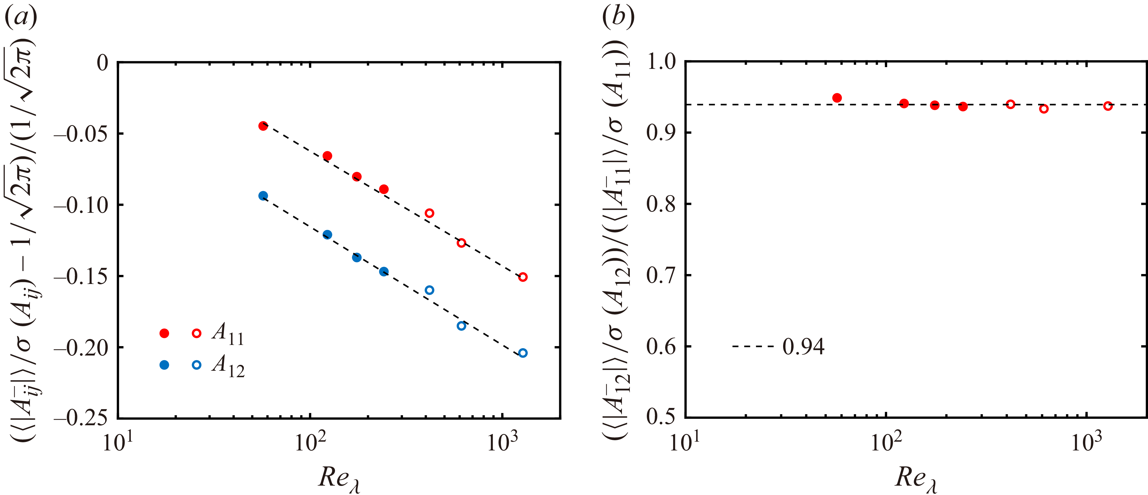
(a) $ \textit{Re}_\lambda$ -dependent relative deviations of the negative-part expectations of $A_{11}$ and $A_{12}$ (normalised by their standard deviations) from that of a Gaussian distribution. In natural log scale, the two dashed lines represent the linear least-squares fits in (3.36) and (3.37), respectively. (b) Ratios between the normalised negative-part expectations of $A_{12}$ and $A_{11}$ . The horizontal dashed line represents the average ratio in (3.38). In both panels, the closed symbols represent results obtained from our DNS at $ \textit{Re}_{\lambda }=57, 123, 175$ and $240$ (cases R1–R4), while the open symbols represent statistics obtained from JHTDB at $ \textit{Re}_{\lambda }=418, 613$ and $1280$ .

We first estimate the non-Gaussian statistics of VGTs in HIT by extracting the longitudinal and transverse VGT components from the fluid phase in our DNS (see § 2). In cases R1–R4, full VGT components $A_{\textit{ij}}$ are sampled at the Eulerian grid points in several snapshots, yielding $3 \times 128^3 \times 100$ , $3 \times 256^3 \times 10$ , $3 \times 384^3 \times 10$ and $3 \times 512^3 \times 10$ samples for $A_{11}$ and twice for $A_{12}$ at $ \textit{Re}_\lambda =57, 123, 175$ and $240$ , respectively. Additionally, we examined the cases with higher $ \textit{Re}_\lambda$ ( $418, 613$ and $1280$ ) from Johns Hopkins Turbulence Database (JHTDB) (Li et al. Reference Li, Perlman, Wan, Yang, Meneveau, Burns, Chen, Szalay and Eyink2008; Yeung et al. Reference Yeung, Donzis and Sreenivasan2012, Reference Yeung, Zhai and Sreenivasan2015) to better show the statistical characteristics in a wide $ \textit{Re}_\lambda$ -range. We calculate the negative-part expectations $\langle |A_{11}^-| \rangle$ and $\langle |A_{12}^-| \rangle$ (normalised by their standard deviations), and compare them with that of a Gaussian distribution, i.e. $1/\sqrt {2\pi }$ . As shown in figure 5(a), both $\langle |A_{11}^-| \rangle$ and $\langle |A_{12}^-| \rangle$ show deviations from the Gaussian approximation which increase with $ \textit{Re}_\lambda$ , and the relative deviation of $A_{12}$ from Gaussianity is always larger than that of $A_{11}$ . Specifically, the impact of non-Gaussianity on the normalised negative-part expectations is relatively small at low $ \textit{Re}_\lambda$ , since the relative deviations of $\langle |A_{11}^-| \rangle$ and $\langle |A_{12}^-| \rangle$ from Gaussianity are $-4.47\,\%$ and $-9.37\,\%$ , respectively, at $ \textit{Re}_\lambda =57$ (case R1). Even at the highest $ \textit{Re}_\lambda =240$ (case R4) in our DNS, the relative deviation of $\langle |A_{11}^-| \rangle$ is only $-8.91\,\%$ from Gaussianity.

Moreover, as shown by the dashed lines in figure 5(a), the linear least-squares fits of the data indicate two scaling laws:

(3.36)

(3.37)

which serve as quantitative predictions of $\langle |A_{11}^-| \rangle$ and $\langle |A_{12}^-| \rangle$ at arbitrary $ \textit{Re}_\lambda$ within the plotted range. Although the normalised negative-part expectations of $A_{12}$ and $A_{11}$ are both $ \textit{Re}_\lambda$ -dependent, their ratio remains almost $ \textit{Re}_\lambda$ -independent, which is observed in both figure 5(b) and the division between (3.36) and (3.37):

(3.38)

\begin{align} \frac {\left \langle \left | A_{12}^- \right | \right \rangle }{\sqrt {\left \langle A_{12}^2 \right \rangle }} \bigg / \frac {\left \langle \left | A_{11}^- \right | \right \rangle }{\sqrt {\left \langle A_{11}^2 \right \rangle }} \approx 0.94. \end{align}

The almost constant ratio in (3.38) indicates that the p.d.f.s of $A_{11}$ and $A_{12}$ possess a statistical self-similarity within the plotted $ \textit{Re}_\lambda$ -range. Since the kinematic collision kernels rely on $\langle |( \unicode{x1D63E}: \unicode{x1D63C})^- | \rangle$ (i.e. the negative-part expectations of the surface-normal relative velocity at collisions), which is a linear combination of both $A_{11}$ and $A_{12}$ , a natural intuition is to find a $ \textit{Re}_\lambda$ -dependent factor to characterise the impact of non-Gaussianity on the collision kernel, with the self-similar $\langle | A_{11}^-| \rangle$ and $\langle | A_{12}^-| \rangle$ evolving with $ \textit{Re}_\lambda$ proportionally to this factor.

Figure 6.

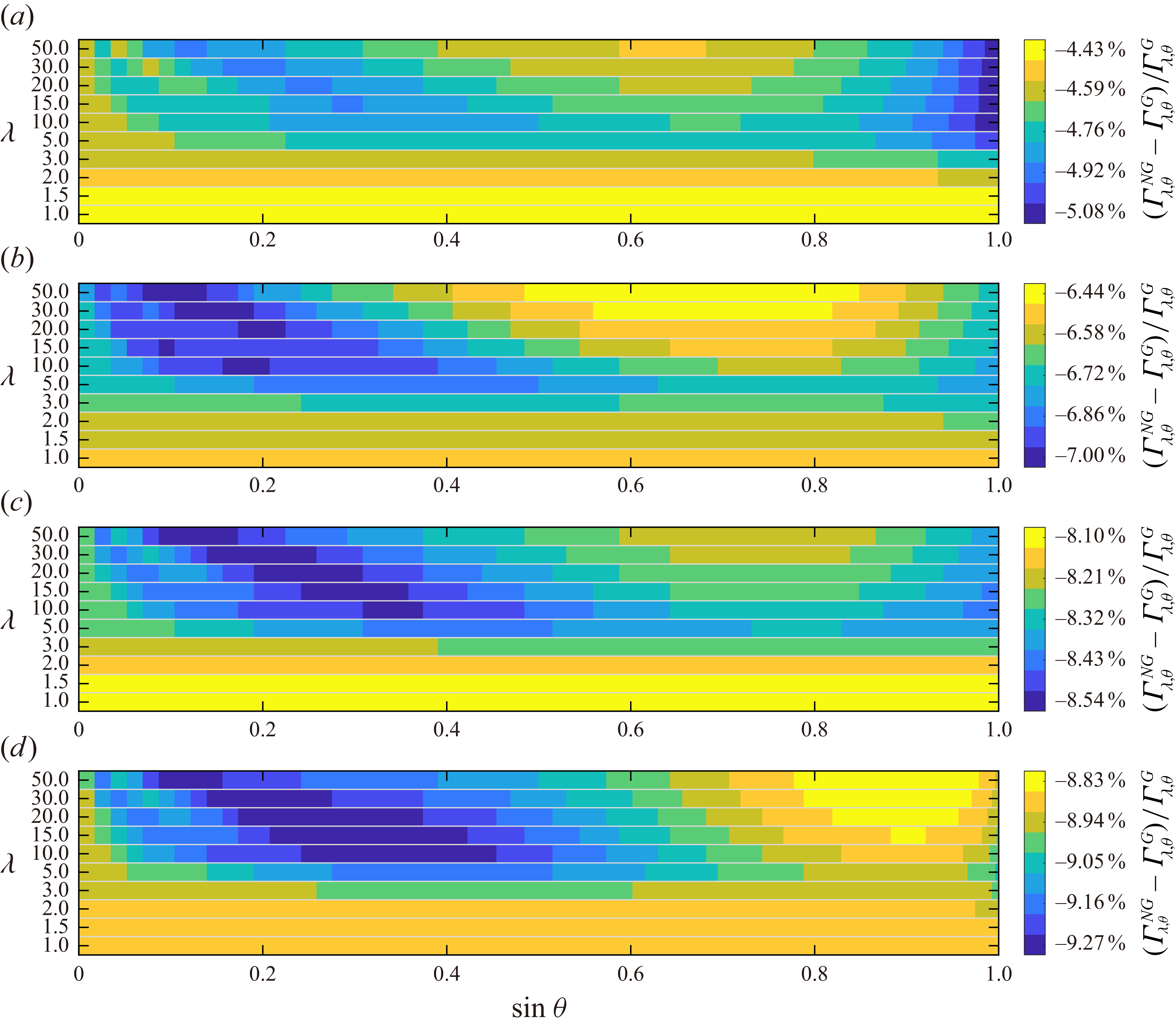
Relative deviations of the non-Gaussian kinematic collision kernels from the Gaussian ones, i.e. $(\varGamma _{\lambda ,\theta }^{\textit{NG}}-\varGamma _{\lambda ,\theta }^{{G}})/\varGamma _{\lambda ,\theta }^{{G}}$ , visualised as contour plots in the ( $\lambda$ , $\sin \theta$ ) parameter space. Panels (a)–(d) correspond to $ \textit{Re}_\lambda =57, 123, 175$ and $240$ (cases R1–R4), respectively.

Therefore, we then construct the non-Gaussian model for the kinematic collision kernels of elongated passive particles, using the VGTs obtained from DNS. Replacing the Gaussian-approximated $\sigma _{zi}/\sqrt {2\pi }$ in (3.16) by the statistical expectations of $( \unicode{x1D63E}_{zi}: \unicode{x1D63C})^-$ , the formulation of the non-Gaussian kinematic collision kernel is expressed as

(3.39)

\begin{align} \varGamma _{\lambda ,\theta }^{\textit{NG}} = 2\sum _{i=1}^{5} \varGamma _{zi}^{\textit{NG}} = 2\sum _{i=1}^{5} \iint _{\varSigma _{zi}}\left \langle \big |( \unicode{x1D63E}_{zi}: \unicode{x1D63C})^- \big | \right \rangle \,\mathrm{d}\varSigma , \end{align}

where the superscript ‘NG’ denotes the non-Gaussian model. Equation (3.39) is calculated numerically through a Monte Carlo approach, directly using adequate samples of VGTs with full components $A_{\textit{ij}}$ extracted from DNS. The relative deviations of the non-Gaussian collision kernels from the Gaussian ones with the same $\lambda$ and $\theta$ , i.e. $(\varGamma _{\lambda ,\theta }^{\textit{NG}}-\varGamma _{\lambda ,\theta }^{{G}})/\varGamma _{\lambda ,\theta }^{{G}}$ , is plotted in figure 6(a–d) at four $ \textit{Re}_\lambda$ . It is found that the non-Gaussianity of VGTs reduce the kinematic collision kernel by limited percentages ( $4.4\,\%{-} 9.3\,\%$ ) in the plotted $ \textit{Re}_\lambda$ -range, with increasing deviations from Gaussianity at higher $ \textit{Re}_\lambda$ , similar to $\langle |A_{11}^-| \rangle$ and $\langle |A_{12}^-| \rangle$ . Furthermore, two features are extracted from the contour plots.

(i) The relative deviations form similar patterns in the ( $\lambda$ , $\sin \theta$ ) parameter space at different $ \textit{Re}_\lambda$ , partly due to the self-similarity between the p.d.f.s of $A_{11}$ and $A_{12}$ in (3.38).
(ii) The relative deviations at a given $ \textit{Re}_\lambda$ vary slightly with $\lambda$ and $\theta$ , indicating that the non-Gaussian impact on the collision kernel is approximately independent of the particle geometry and relative alignment. This observation justifies the use of a single $ \textit{Re}_\lambda$ -dependent non-Gaussianity factor to characterise the non-Gaussian impact on the kinematic collision kernel. Moreover, the relative deviations from Gaussianity are adequately close to those of $\langle |A_{11}^-| \rangle$ , compared with $\langle |A_{12}^-| \rangle$ , which further supports the approximate non-Gaussianity factor:

(3.40)

\begin{align} \mathcal{K}^{\textit{NG/G}} = \frac {\left \langle \left | A_{11}^- \right | \right \rangle }{\sqrt {\left \langle A_{11}^2 \right \rangle }} \bigg / \frac {1}{\sqrt {2\pi }} = -0.0346\ln Re_\lambda + 1.10, \end{align}

dependent only on $ \textit{Re}_\lambda$ . The non-Gaussian collision kernels at arbitrary $ \textit{Re}_\lambda$ within the present range can therefore be directly obtained from the Gaussian ones by

(3.41)

\begin{align} \varGamma _{\lambda ,\theta }^{\textit{NG}} \approx \mathcal{K}^{\textit{NG/G}} \varGamma _{\lambda ,\theta }^{{G}}. \end{align}

In Appendix B, we provide a further justification for the use of $\langle |A_{11}^-| \rangle$ as the non-Gaussianity factor.

In summary of this section, we first construct the Gaussian model for kinematic collision kernels, where figure 3 and the approximation (3.35) demonstrate the profile of $\varGamma _{\lambda ,\theta }^{{G}}$ with arbitrary relative angles and aspect ratios. Further introducing the non-Gaussian model, figure 6 demonstrates the $ \textit{Re}_\lambda$ -dependent but limited errors due to the non-Gaussianity of VGTs, and a non-Gaussianity factor $\mathcal{K}^{\textit{NG/G}}$ is proposed in (3.40) to obtain the non-Gaussian collision kernels $\varGamma _{\lambda ,\theta }^{\textit{NG}}$ directly from the Gaussian-approximated $\varGamma _{\lambda ,\theta }^{{G}}$ , at any $ \textit{Re}_\lambda$ .

Unaffected by the non-Gaussianity, we observe a consistently positive correlation between the present collision kernel $\varGamma _{\lambda ,\theta }$ and the relative angle $\theta$ , which is approximately proportional to $\sin \theta$ for highly elongated particles. Specifically, at $\lambda =20$ , the collision kernel of perpendicular pairs is approximately sixfold higher than that of the parallel pairs. In other words, if two subsets of particles with identical number density are considered at the limits $\theta \rightarrow 0$ and ${\pi }/{2}$ , substantially more collisions would happen with perpendicular relative alignment, while parallel alignment suppresses collisions. However, elongated nearby particles in turbulence tend to align with the identical direction of Lagrangian fluid stretching (Pumir & Wilkinson Reference Pumir and Wilkinson2011; Chevillard & Meneveau Reference Chevillard and Meneveau2013; Ni, Ouellette & Voth Reference Ni, Ouellette and Voth2014; Zhao et al. Reference Zhao, Gustavsson, Ni, Kramel, Voth, Andersson and Mehlig2019), intuitively leading to more collisions with parallel alignment. It could be speculated that, except for the collision kernel with fixed relative angles, the non-uniform distribution of the relative angles between nearby particle pairs is essential to be considered in the theoretical model.

3.2. Angular probability distribution of nearby pairs

Given the above-mentioned analyses, we further illustrate the probability of elongated nearby particle pairs with specific relative angles. This p.d.f. is obtained from DNS for elongated passive particles in HIT with $ \textit{Re}_{\lambda } =57$ .

In DNS, we focus on the potentially colliding pairs, which are technically classified as neighbours if their relative angles and interparticle distances satisfy the conditions $\theta ^{(i)}-\Delta \theta /2 \lt \theta \lt \theta ^{(i)}+\Delta \theta /2$ and $0 \lt \delta \lt \Delta \delta$ , respectively, where we set $\Delta \theta = \pi /1800$ and $\Delta \delta = 0.01a$ . In other words, the centre of one particle is located inside a thin layer with a thickness $\Delta \delta$ over the contact region of a neighbouring particle, with their relative angle in a small neighbourhood of the sampling angle $\theta ^{(i)}$ . By counting the total number of the afore-defined neighbouring pairs $N_{\textit{neig},\theta ^{(i)}}$ in the simulation, averaged over sufficient samples, the angular-volumetric number density of neighbouring pairs is calculated by

(3.42)

\begin{align} n_{\lambda ,\theta ^{(i)}}=\frac {1}{\Delta \theta }\frac {N_{\textit{neig},\theta ^{(i)}}/N_{\textit{pair}}}{\mathcal{A}_{\varSigma }\Delta \delta /V}, \end{align}

which is normalised by the number density of all particle pairs. Here, $N_{\textit{pair}} = N_{\textit{part}}^2/2$ is the total amount of pairs in the computation domain with volume $V$ , and is the surface area of the contact region.

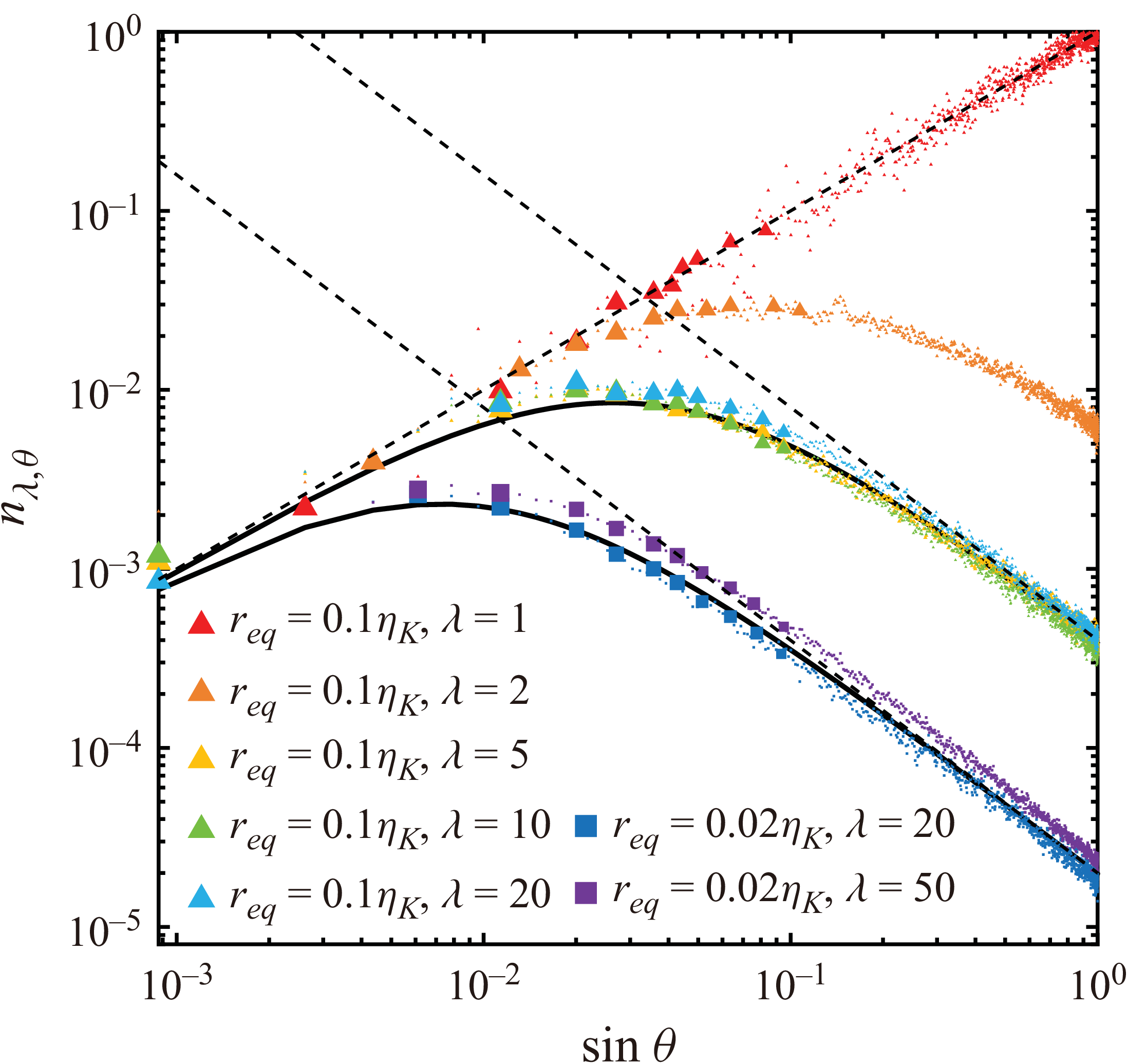
We consider seven particle configurations with various aspect ratios ( $\lambda =1 \sim 50$ ) and equivalent radii ( $r_{\textit{eq}}=0.1\eta _{{K}}$ and $0.02\eta _{{K}}$ ). The normalised angular-volumetric number density $n_{\lambda ,\theta }$ is plotted by coloured scatters in figure 7, revealing the angular p.d.f. of the relative angle between neighbouring pairs. We find $n_{\lambda ,\theta } \approx \sin \theta$ for elongated pairs with small relative angles, similar to the spherical tracers with independently and identically random orientations which lead to $n_{\lambda =1,\theta } = \sin \theta$ (verified by the red scatters). However, a considerable decrease by $2{-} 4$ orders of magnitude in $n_{\lambda ,\theta }$ is found at large relative angles for elongated particles, compared with the spherical ones. For highly elongated particles with $\lambda \geq 5$ , the angular p.d.f.s remain almost the same regardless of the aspect ratio, where we observe a rise when $\theta$ increases from 0, followed by a peak around $\sin \theta =10^{-2} \sim 10^{-1}$ and then a steep descent. Two distinct power laws are recognised in both the small- and large-relative-angle regimes:

(3.43)

\begin{align} n_{\lambda ,\theta }(r_{\textit{eq}},\lambda ;\theta )=\left \{ \begin{array}{ll} n_{\lambda ,\theta }^{\parallel } \approx \sin \theta , & 0\lt \sin \theta \lesssim 10^{-2},\\[5pt] n_{\lambda ,\theta }^{\perp } \approx c_{\lambda }^{\perp }(\sin \theta )^{-1.3}, & 10^{-1} \lesssim \sin \theta \lt 1, \\ \end{array} \right . \end{align}

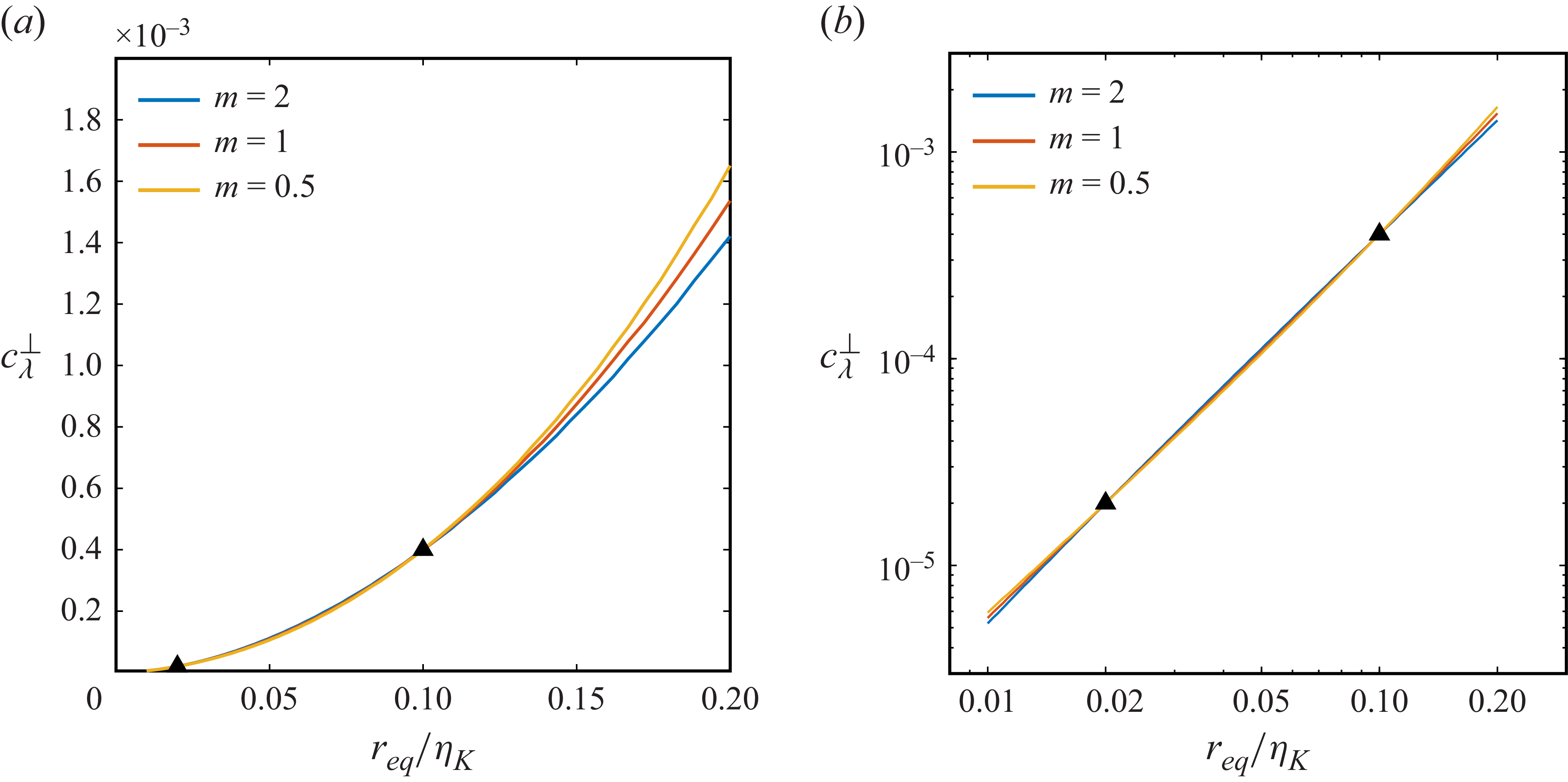
shown by dashed lines in figure 7. The exponents are found almost independent of the equivalent radius, with the parameter $c_{\lambda }^{\perp }=4\times 10^{-4}$ and $2\times 10^{-5}$ for $r_{\textit{eq}}=0.1\eta _{{K}}$ and $0.02\eta _{{K}}$ , respectively. For generalisation, $c_{\lambda }^{\perp }$ can be easily extended to particles with any sub-Kolmogorov size, according to $c_{\lambda }^{\perp } \propto (r_{\textit{eq}}/\eta _{{K}})^{1.86}$ (see Appendix C for details). We fit all the scatters by

(3.44)

\begin{align} n_{\lambda ,\theta }(r_{\textit{eq}},\lambda ;\theta ) = \left [\left (n_{\lambda ,\theta }^{\parallel }\right )^k+\left (n_{\lambda ,\theta }^{\perp }\right )^k \right ]^{{1}/{k}},\,\,\,\,\lambda \geq 5,\,\theta \in \left [0,\frac {\pi }{2}\right ], \end{align}

where $k=-1/2$ , and the results are plotted by solid curves in figure 7, applicable to all relative angles. Moreover, the non-monotonic variation of $n_{\lambda ,\theta }$ provides the detailed angular structure of neighbouring particles’ relative alignment. The leftward shift trend of the curves reflects an increasing tendency for the neighbouring pairs to align with each other as their elongation grows. As a direct evidence, the statistics at $ \textit{Re}_{\lambda } =57$ and $\lambda =5$ indicate that up to 38.4 % of collisions happen with $|\boldsymbol{p}_1 \boldsymbol{\cdot }\boldsymbol{p}_2|=\cos \theta \gt 0.99$ , but only 5.3 % with $\cos \theta \lt 0.2$ .

Figure 7.

The normalised angular-volumetric number density $n_{\lambda ,\theta }$ of neighbouring pairs with different equivalent radii $r_{\textit{eq}}$ and aspect ratios $\lambda$ , as functions of $\sin \theta$ . The number density of spherical particles is scaled by $n_{\lambda =1,\theta =\pi /2}$ , while all distributions are vertically shifted to the same level at $\theta \rightarrow 0$ , without any impact on the subsequent calculation of the collision kernel. The sizes of scatters are adjusted only for the sake of visualisation. In the log–log scale, the dashed lines represent the power laws in (3.43) and the fitting results of (3.44) are shown by the solid curves.

3.3. Overall collision kernel

Using the theoretical collision kernels with fixed relative angles in § 3.1 and the p.d.f.s of the relative angles between neighbouring pairs in § 3.2, we finally close the theoretical expressions of the overall kinematic collision kernels $\varGamma _{\lambda }$ for elongated passive particles in HIT, by integration and discrete summation separately:

(3.45)

\begin{align} \varGamma _{\lambda }(r_{\textit{eq}},\lambda ) = \frac {\int _0^{{\pi }/{2}} \varGamma _{\lambda ,\theta } n_{\lambda ,\theta } \mathrm{d}\theta }{\int _0^{{\pi }/{2}} n_{\lambda ,\theta } \mathrm{d}\theta } \approx \frac {\sum \varGamma _{\lambda ,\theta ^{(i)}} n_{\lambda ,\theta ^{(i)}}}{\sum n_{\lambda ,\theta ^{(i)}}}. \end{align}

For the Gaussian model aimed at $\varGamma _{\lambda }^{{G}}$ , the summation form involves $\varGamma _{\lambda ,\theta ^{(i)}}^{{G}}$ directly from (3.16) and the DNS-based $n_{\lambda ,\theta ^{(i)}}$ in (3.42), both at the sampling angle $\theta ^{(i)}$ ; while the integration form adopts the fitting results in (3.35) and (3.44) validated for $\lambda \geq 5$ . As for the non-Gaussian model aimed at $\varGamma _{\lambda }^{\textit{NG}}$ , we simply use the summation form by adopting $\varGamma _{\lambda ,\theta ^{(i)}}^{\textit{NG}}$ from (3.39) and the same DNS-based $n_{\lambda ,\theta ^{(i)}}$ .

For comparison, we calculate the dynamic collision kernels by DNS data, according to the statistically averaged formulation of (1.1):

(3.46)

\begin{align} \varGamma _{\lambda }^{{d}} = \frac {2N_{\textit{coll}}V}{N_{\textit{part}}^2 T}, \end{align}

where $N_{\textit{coll}}$ is the total number of collisions recorded in the simulation with volume $V$ , during a sampling time window $T$ .

Figure 8.

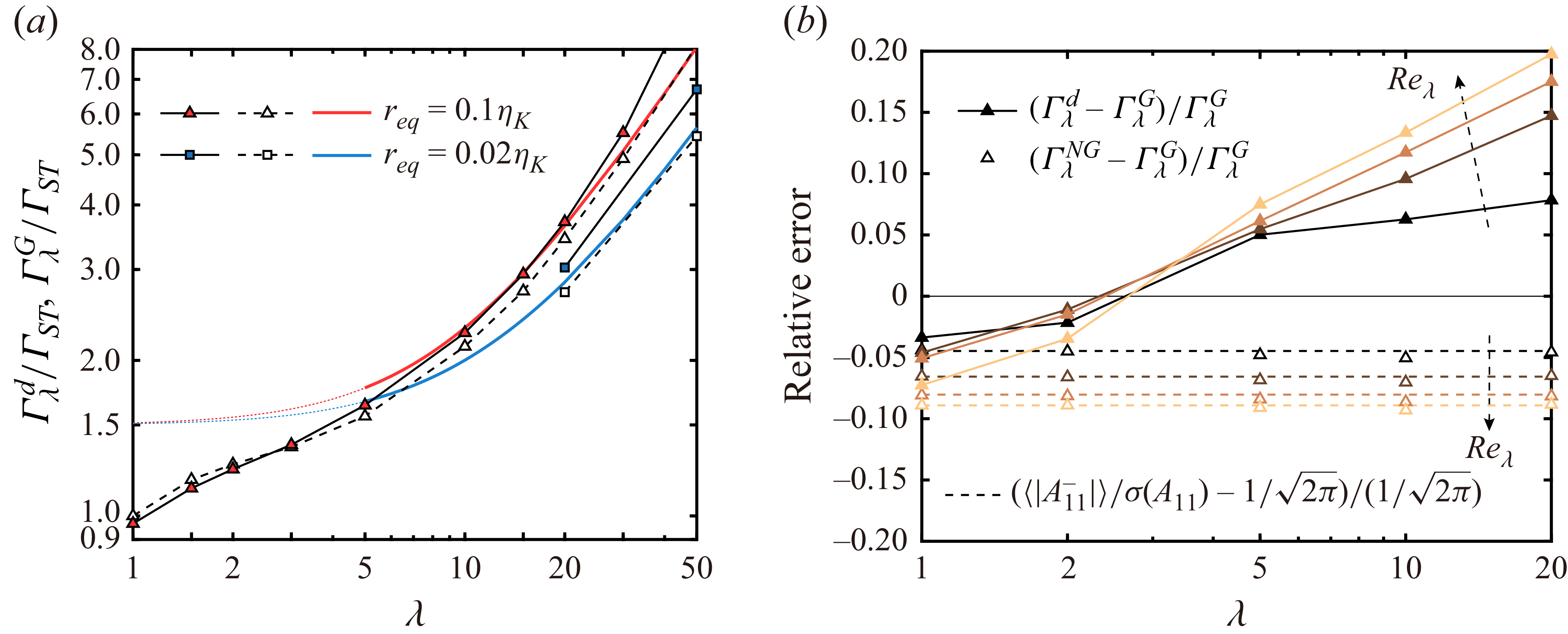
(a) Kinematic collision kernel ratios $\varGamma _{\lambda }^{{G}}/\varGamma _{\textit{ST}}$ (predicted by the Gaussian model) separately yielded by the integration form (coloured curves) and the summation form (open symbols) in (3.45), compared with the dynamic kernel ratios $\varGamma _{\lambda }^{{d}}/\varGamma _{\textit{ST}}$ (closed symbols) obtained from DNS at $ \textit{Re}_{\lambda } =57$ . (b) Relative errors of the dynamic collision kernels and the non-Gaussian kinematic collision kernels with respect to the Gaussian ones, i.e. $(\varGamma _{\lambda }^{{d}}-\varGamma _{\lambda }^{{G}})/\varGamma _{\lambda }^{{G}}$ (closed symbols) and $(\varGamma _{\lambda }^{\textit{NG}}-\varGamma _{\lambda }^{{G}})/\varGamma _{\lambda }^{{G}}$ (open symbols) at $ \textit{Re}_{\lambda }=57, 123, 175$ and $240$ (increasing along the arrows) and $r_{\textit{eq}}=0.1\eta _{{K}}$ . The horizontal dashed lines show the corresponding relative deviations of $\langle |A_{11}^-| \rangle /\sigma (A_{11})$ from Gaussianity in (3.36).

First, we estimate the accuracy of the Gaussian model. The kinematic and dynamic collision kernels of elongated passive particles in HIT are plotted in figure 8(a), where the open symbols and solid curves stand for the results of the summation and integration forms in (3.45), respectively. We observe that the kinematic collision kernels obtained by both forms of the Gaussian model are in good agreement with the dynamic ones from DNS at $ \textit{Re}_{\lambda } =57$ (shown by the closed symbols), despite the relatively large errors in extremely large aspect ratios ( $\lambda \gt 20$ ). There are three main approximations or hypotheses that may contribute to this mismatch.

(i) The formulation $ \unicode{x1D63E}: \unicode{x1D63C}$ in (3.6) is a first-order expansion of the surface-normal relative velocity at one of the particle centres, which is applicable only when the separation distance between the two particle centres is smaller than $\eta _{{K}}$ at collisions. For particles with $r_{\textit{eq}}=0.1\eta _{{K}}$ and $\lambda \gt 20$ , the major-axis length of particles exceeds $1.5\eta _{{K}}$ , making the first-order approximation less accurate.
(ii) The derivations to obtain $\langle |( \unicode{x1D63E}: \unicode{x1D63C})^- | \rangle$ implicitly assume that the VGTs $ \unicode{x1D63C}$ remain statistically isotropic in the particle frame $(x,y,z)$ shown in figure 1(b), which is not the fact due to the aforementioned preferential alignment of elongated particles with the Lagrangian fluid stretching directions, especially for extremely elongated ones.
(iii) $n_{\lambda ,\theta }$ is defined as a layer-averaged number density of neighbouring particle centres in (3.42), while the local number density $n_{\lambda ,\theta }(\boldsymbol{x}_2)$ ( $\boldsymbol{x}_2 \in \varSigma$ ) can in fact vary across $\varSigma$ , especially for extremely elongated particles. However, this spatial non-uniformity is neglected in the present theoretical model (3.45). Additionally, the $ \textit{Re}_\lambda$ -dependence of $n_{\lambda ,\theta }$ is not yet examined.

Nevertheless, the overall good agreement in figure 8(a) validates the Gaussian model as a reasonable baseline for predicting the collision kernels, and the finite impacts attributed to approximations (i)–(iii) are briefly discussed in § 4.

Then, we further estimate the accuracy and $ \textit{Re}_\lambda$ -dependence of the non-Gaussian model. Figure 8(b) quantifies the relative errors of the dynamic kernels and the non-Gaussian kinematic kernels with respect to the Gaussian ones (calculated by the summation form). At all four $ \textit{Re}_\lambda$ , the relative errors of the non-Gaussian kinematic kernels shown by the open symbols, $(\varGamma _{\lambda }^{\textit{NG}}-\varGamma _{\lambda }^{{G}})/\varGamma _{\lambda }^{{G}}$ , are negative and almost independent of $\lambda$ , with magnitudes of approximately $4.4\,\% {-} 9.3\,\%$ that increase with $ \textit{Re}_{\lambda }$ . These open symbols nearly collapse onto the horizontal dashed lines representing the relative deviations of $\langle |A_{11}^-| \rangle /\sigma (A_{11})$ from Gaussianity, which comfirms that the non-Gaussianity factor defined in (3.40) further provides an accurate estimation of the overall kinematic collision kernel predicted by the non-Gaussian model:

(3.47)

\begin{align} \varGamma _{\lambda }^{\textit{NG}} \approx \mathcal{K}^{\textit{NG/G}} \varGamma _{\lambda }^{{G}}. \end{align}

In contrast, the relative errors of the dynamic kernels shown by the closed symbols, $(\varGamma _{\lambda }^{{d}}-\varGamma _{\lambda }^{{G}})/\varGamma _{\lambda }^{{G}}$ , change signs from negative to positive as $\lambda$ grows. Specifically, for spherical tracers ( $\lambda =1$ ), the dynamic collision kernels are lower than the Gaussian kinematic collision kernels with magnitudes of approximately $3.4\,\% {-} 7.3\,\%$ that increase with $ \textit{Re}_{\lambda }$ , and are consistent in trend but slightly higher than the non-Gaussian kernels. Similar negative errors are found in the regime with $1\leq \lambda \lesssim 3$ , which indicates that the non-Gaussian model captures the non-Gaussianity effects of VGTs and provides better predictions of the dynamic kernels for spherical-like elongated particles than the Gaussian model. However, for $\lambda \gtrsim 3$ , both the Gaussian and non-Gaussian models underestimate the dynamic kernels, with the relative errors growing monotonically with $\lambda$ and $ \textit{Re}_\lambda$ . We notice that, at relatively low $ \textit{Re}_\lambda$ (e.g. $ \textit{Re}_\lambda =57$ ), the Gaussian model already provides good predictions of the dynamic kernels for highly elongated particles with $\lambda$ up to 20, with relative errors less than $8\,\%$ .

As discussed in § 4, the first-order approximation (i) introduces an almost $ \textit{Re}_\lambda$ -independent impact, which could partly explain the underestimations of the present models when applied to extremely elongated particles at low $ \textit{Re}_\lambda$ . Moreover, the errors introduced by hypotheses (ii) and (iii) are expected to be positively correlated with $\lambda$ and $ \textit{Re}_\lambda$ due to the increasing anisotropy of $ \unicode{x1D63C}$ and non-uniformity of $n_{\lambda ,\theta }(\boldsymbol{x}_2)$ in the particle frame.

Despite the systematic errors when predicting by the Gaussian and non-Gaussian models, an obvious positive correlation is found between the collision kernel and aspect ratio, indicating that elongated particles collide with each other more frequently than equal-volume spherical tracers in turbulence, which is consistent with the previous findings (Arguedas-Leiva et al. Reference Arguedas-Leiva, Słomka, Lalescu, Stocker and Wilczek2022; Grujić et al. Reference Grujić, Bhatnagar, Sardina and Brandt2024). However, by decomposing the collision kernel, our theoretical collision model identifies two competing effects induced by particle elongation effect, i.e. the increase in $\varGamma _{\lambda ,\theta }$ , which enhances collisions, and the leftward shift in the distribution of $n_{\lambda ,\theta }$ , which aligns the neighbouring pairs and suppresses their collisions as elongation grows. The monotonically increasing trend of $\varGamma _{\lambda }$ in figure 8(a) reveals that the enhancement effect is the dominant factor. Nevertheless, it remains important to elucidate the relative alignment mechanism of the elongated colliding pairs, using nearby particle statistics (see § 3.4).

3.4. Physics of the aligning process

To clarify the physics of the aligning process of colliding pairs with different relative angles at collisions, we investigate their history effect by tracking them backward over several Kolmogorov time scales $\tau _{\eta }$ prior to collisions.

Figure 9.

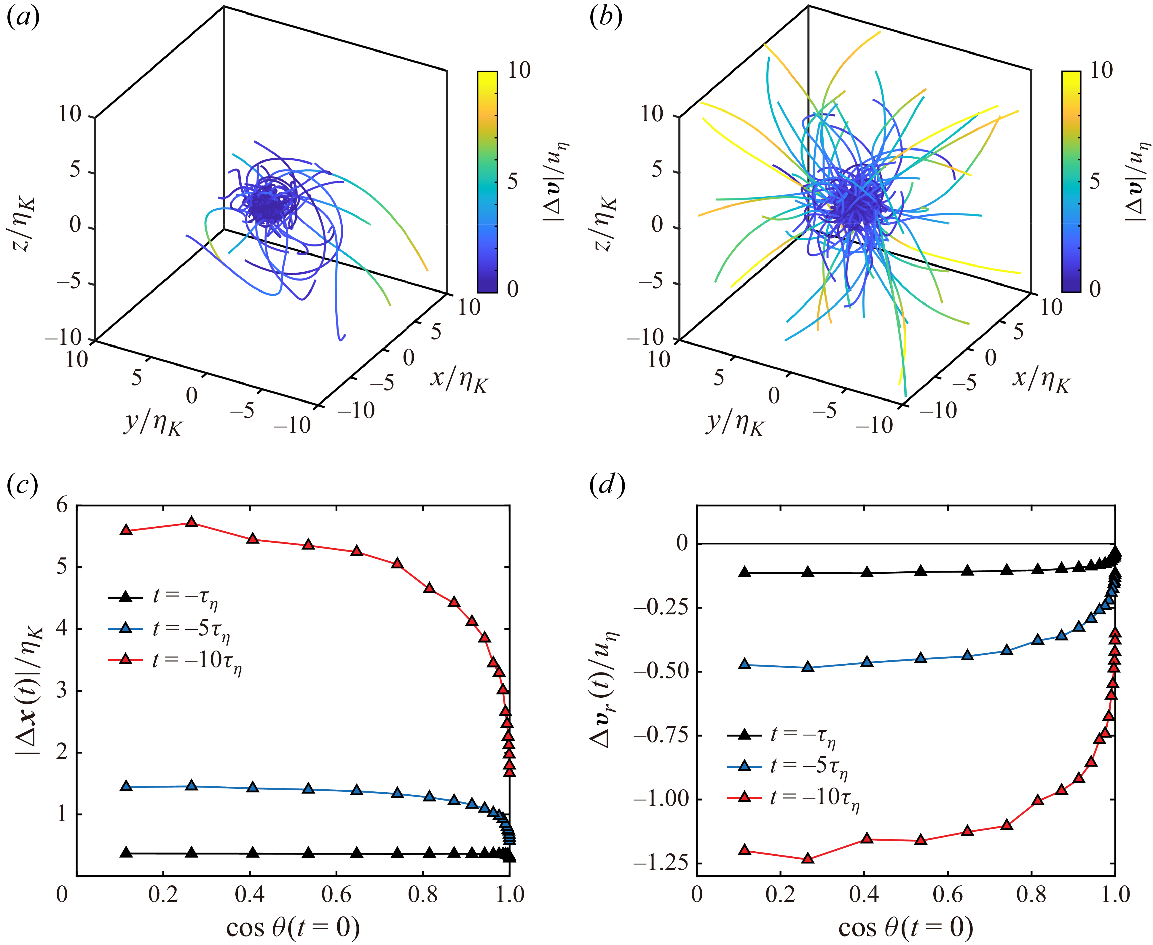
Trajectories of one particle with $\lambda = 5$ relative to another (fixed at the origin) in 200 colliding pairs, tracked over $10\tau _{\eta }$ before colliding with (a) $\cos \theta \gt 0.99$ and (b) $\cos \theta \lt 0.2$ . Colours represent the relative velocity $|\varDelta \boldsymbol{v}|$ between particle pairs, normalised by the Kolmogorov velocity scale $u_{\eta }=\eta _{{K}}/\tau _{\eta }$ . (c) Separation distance $|\Delta \boldsymbol{x}(t)|$ and (d) radial relative velocity $\Delta v_{r}(t)$ (negative stands for approaching) of 200 000 colliding pairs at $\tau _{\eta }$ , $5\tau _{\eta }$ , $10\tau _{\eta }$ before collisions. The triangular symbols mark the means of every 5 % segment, as functions of $\cos \theta$ at the collision instant $t=0$ . Here, $ \textit{Re}_{\lambda } =57$ .

Figure 9(a,b) illustrates the trajectories of single elongated particles in $10\tau _{\eta }$ before colliding with almost parallel and perpendicular relative alignment, respectively, transformed into the frames of their collision partners. We find remarkable differences in the separation distance and relative velocity induced by turbulent dispersion, with the perpendicular pairs exhibiting greater separation and higher relative velocity than that of the parallel pairs. As for collisions with general relative angles, weak correlations are observed between the historical separation distance $|\Delta \boldsymbol{x}(t)|$ and $\cos \theta$ at the collision instant if $\theta \gt \pi /4$ , followed by steep declines as the colliding pairs tend to align with each other (see figure 9 c). Similar trends are found in the radial relative velocity $\Delta v_{r}(t)$ in figure 9(d), indicating that parallel colliding pairs undergo less dispersion in both velocity and distance compared with the perpendicular ones, thereby allowing more time to align with the local fluid vorticity if approaching from the same initial separation distance (Parsa et al. Reference Parsa, Guasto, Kishore, Ouellette, Gollub and Voth2011; Ni et al. Reference Ni, Ouellette and Voth2014; Zhao & Andersson Reference Zhao and Andersson2016). Conversely, perpendicular pairs require a significantly higher approaching velocity to encounter. Since large local velocity differences are of little possibility in HIT, those perpendicular pairs are less likely to neighbour each other, explaining the reduction in $n_{\lambda ,\theta }$ for elongated neighbouring pairs with large relative angles.

We emphasise that the discussion here is restricted to inertialess particles with relative motions governed by the radial relative velocity on large scales and local velocity gradients when approaching. When particle inertia is non-negligible, inertialess hydrodynamics and near-contact dynamics may alter the statistical observations.

3.5. Statistics of the collision states

While the theory, statistics and phenomena discussed previously are mainly based on the relative angles, more detailed information concerning the relative positions of particle centres and colliding points is also crucial in the analyses of the collision process.

Figure 10.

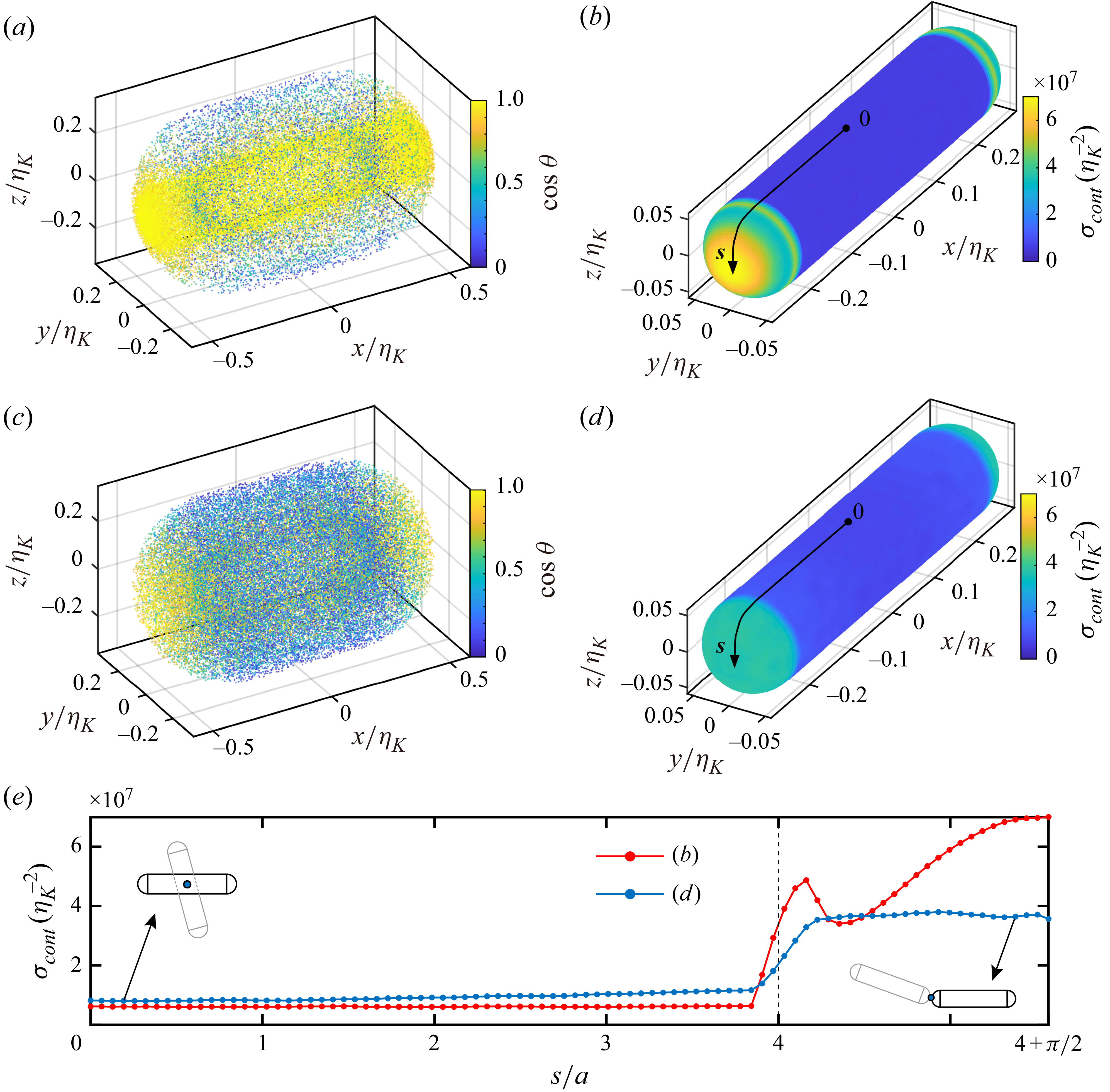
(a) Relative positions of particle centres with $\lambda = 5$ at the collision instant. The scatters are coloured by $\cos \theta$ . (b) Contour of the areal density of colliding points $\sigma _{\textit{coll}} = \Delta N_{\textit{coll}}/\Delta \mathcal{A}_{\mathrm{s}}$ , calculated by the count of collisions in per unit area of the particle surface. Strong aggregations appear in parallel collisions (yellow scatters in figure 10 a) and edge-to-edge collisions (yellow regions in figure 10 b), compared with (c,d) the non-rotational tracers with orientations randomly initialised and rotation turned off. (e) Cross-section view of $\sigma _{\textit{coll}}$ along the curve $\boldsymbol{s}$ . Here, $ \textit{Re}_{\lambda } =57$ .

We record 200 000 collisions for each particle configuration in DNS, and plot the three-dimensional relative positions of particle centres and the areal density $\sigma _{\textit{coll}}$ of colliding points in figure 10(a,b), respectively, both in the particle frame. By contrast, additional simulations of non-rotational tracers are conducted, in which we artificially turn off the rotation of particles but keep their translational motion. The corresponding results are presented in figure 10(c,d).

Apart from the anomalously large proportion of parallel collisions (represented by yellow scatters), the scatters of particle centres are found much denser close to the symmetry axis. Meanwhile, we observe an aggregation of colliding points on the spherical caps of particles, compared with non-rotational tracers. The variation of $\sigma _{\textit{coll}}$ along the curve $\boldsymbol{s}$ is plotted in figure 10(e). Despite the peaks at both ends of the sidewall, the maximum areal density lies exactly at the edge points, one order of magnitude higher than on the sidewall. Furthermore, $\sigma _{\textit{coll}}$ at the edge points is also twofold higher than the maximum for non-rotational tracers. Therefore, elongated passive particles tend to engage in parallel and edge-to-edge collisions in HIT, primarily attributable to their rotational dynamics.

This is probably an explanation for the chain-formation process of elongated phytoplankton in aquatic environments (Fraga, Gallager & Anderson Reference Fraga, Gallager and Anderson1989; Park et al. Reference Park, Jeong, Lee, Cho and Kwon2001; Smayda Reference Smayda2010; Sohn et al. Reference Sohn, Seo, Choi, Lee, Kang and Kang2011). Our explanation is a fundamental one as we introduce a mechanism of parallel and edge-to-edge collisions between passive particles in turbulence, which is validated for physical particles only when they are far from contact, or when the near-contact hydrodynamic interactions are negligible or restricted to very short ranges. By further involving real interactions between particles, such as lubrication and adhesion, the preferential collision states found in the present paper are expected to be verified or further corrected.

4. Conclusions and outlooks

A theoretical framework is established to estimate the collision kernels $\varGamma _{\lambda }$ for elongated passive particles in HIT. The overall collision kernels are composed of two decisive terms as follows. First, $\varGamma _{\lambda ,\theta }$ is proposed to quantify the collision kernels of particles with fixed relative angles at the collision instant, while $\varGamma _{\lambda ,\theta }^{{G}}$ is theoretically derived under the Gaussian hypothesis of VGTs and is extended to $\varGamma _{\lambda ,\theta }^{\textit{NG}}$ by introducing an $ \textit{Re}_\lambda$ -dependent non-Gaussianity factor. Then $n_{\lambda ,\theta }$ is obtained from DNS data and represents the angular p.d.f.s of the relative angles of the neighbouring pairs. The overall collision kernels are therefore calculated separately by the summation and integration forms, also incorporating the Gaussian and non-Gaussian models. Additionally, to interpret the non-monotonic variations of $n_{\lambda ,\theta }$ , we study the history effect of the colliding pairs with different relative angles and clarify the physics of their aligning behaviour.

Our model can reliably provide the collision kernels of elongated particles in turbulence, with the generalisation ability in a wide range of aspect ratio, particle size and Reynolds number, despite the relatively large errors in large aspect ratio and high- $ \textit{Re}_\lambda$ cases. Here, we comment on the impact of the three approximations and hypotheses mentioned in § 3.3, and discuss possible improvements for future studies.

(i) The first-order expansions of the surface-normal relative velocity at the particle centres. We examine the contribution ratios of the $m$ th-order longitudinal fluid velocity gradients to the RRV of two points with a separation distance $R$ , normalised by that of the first-order longitudinal velocity gradient:

(4.1)

\begin{align} \mathcal{P}_m(R)= \frac {R^{m-1}}{m!\langle | A_{11}^- | \rangle } \left \langle \left | \left ( \frac {\partial ^m u_1}{\partial x_1^m} \right )^- \right | \right \rangle \propto R^{m-1}. \end{align}

The ratios with $m=2,3,4$ and $R=\eta _{{K}}$ are listed in table 3 at various $ \textit{Re}_{\lambda }$ , which indicate that the contribution of the second-order fluid velocity gradients (i.e. the velocity Hessian) is not negligible for Kolmogorov-scale particles, since two elongated particles with the major-axis length exceeding $\eta _{{K}}$ could collide with a separation distance $R\gt \eta _{{K}}$ . Another observation is that the contribution ratios are almost $ \textit{Re}_{\lambda }$ -independent, which comfirms the finite errors caused by the neglected higher-order terms when the present model is applied to high- $ \textit{Re}_\lambda$ HIT.

Table 3.

Contribution ratios $\mathcal{P}_m(R)$ of the second-, third- and fourth-order longitudinal fluid velocity gradients to the RRV with a separation distance $R=\eta _{{K}}$ , obtained from DNS at $ \textit{Re}_{\lambda }=57, 123, 175$ and $240$ (cases R1–R4).

Involving the velocity Hessian in the model requires more complicated derivations and adequate statistics from DNS, and thus is left for future work.

(ii) The anisotropy of VGTs in the particle frame. In the derivations of the Gaussian model and the Monte Carlo approach for the non-Gaussian model, calculating $\langle |( \unicode{x1D63E}: \unicode{x1D63C})^-| \rangle$ relies on the isotropy of $A_{\textit{ij}}$ in the particle frame identical to that in the Eulerian frame. However, the real VGTs $ \unicode{x1D63C}^\ast$ correlate with the particle orientations, which potentially affects the statistics of $ \unicode{x1D63E}: \unicode{x1D63C}^\ast$ .

We try to interpret the limited impact of this anisotropy by a general explanation. Similar to Appendix B, one may diagonalise $ \unicode{x1D63E}$ at each point on the contact region surface, so that $ \unicode{x1D63E}: \unicode{x1D63C}^\ast = \unicode{x1D63E}^\prime : \unicode{x1D63C}^{\ast \prime }$ becomes a linear combination of $A^{\ast \prime }_{11}$ , $A^{\ast \prime }_{22}$ and $A^{\ast \prime }_{33}$ . Although the anisotropy of $ \unicode{x1D63C}^{\ast \prime }$ remains, the collision kernel formulation (3.7) involves a surface integration of $\langle ( \unicode{x1D63E}: \unicode{x1D63C}^\ast )^-\rangle$ over the whole contact region, where $ \unicode{x1D63C}^{\ast \prime }$ is obtained from $ \unicode{x1D63C}^\ast$ transformed into various principal coordinates of $ \unicode{x1D63E}$ , with its anisotropic effect partially averaged out. Nevertheless, a quantitative analysis on the impact of this anisotropy would be a natural refinement of the present model.

(iii) The hypothesis of spatially uniform $n_{\lambda ,\theta }$ . Strictly, the exact collision kernel with a fixed relative angle can be formulated as an integration of the local collision flux on the contact region surface:

(4.2)

and the exact overall collision kernel is therefore

(4.3)

whereas formulations (3.1) and (3.45) replace the position-dependent $n_{\lambda ,\theta }(\boldsymbol{x}_2)$ ( $\boldsymbol{x}_2 \in \varSigma$ ) by its layer-averaged value $n_{\lambda ,\theta }$ .

Hypothesis (iii) also incurs limited errors. For example, we estimate on elongated particles with $\lambda =5$ that the ratio of number density at the edge points of the contact region surface to that on the sidewall is $n_{\lambda ,\theta }(\boldsymbol{x}_{2,\textit{edge}})/n_{\lambda ,\theta }(\boldsymbol{x}_{2,\textit{side}}) \approx 1.15$ , only slightly higher than unity. Nevertheless, a more refined and position-resolved description of $n_{\lambda ,\theta }(\boldsymbol{x}_2)$ would be a natural extension of the present theory, especially for particles with extremely elongated or more complex geometry.

As a final remark, the present theoretical model also provides insights into other granular matters in turbulence except for collision rate predictions, including the chain-formation mechanism of phytoplankton. Extending the present approach to include bidisperse or polydisperse particle collisions would be essential to quantitatively describe the nature of chain-formation. Furthermore, the impacts of near-contact hydrodynamic interactions between elongated particles on their collision kernels and behaviours remain worthy of future exploration. With the subsequent implementation of our theoretical collision model, more applications such as forecasting the phytoplankton blooms (Burd & Jackson Reference Burd and Jackson2009) and rainfall/snowfall (Phillips et al. Reference Phillips, Formenton, Bansemer, Kudzotsa and Lienert2015; Chandrakar et al. Reference Chandrakar, Morrison, Grabowski and Lawson2024) are expected.

Funding

This work is supported by the National Natural Science Foundation of China (Grant Nos. 125B1013, 12532011, 12388101 and 12472224) and Xingjian College (College of Future Technology) Future Technology Challenge Project. The authors also acknowledge the support by State Key Laboratory of Advanced Space Propulsion (No. 2025ASP0101).

Declaration of interests

The authors report no conflict of interest.

Appendix A. Collision detection algorithm in DNS

For each particle pair that potentially collides, we need to find the minimal distance $d_{\textit{min}}$ between the two symmetry axes (represented by dashed lines in figure 11). With the normalised parameters $s_1,s_2\in [-1,1]$ , the coordinates of points located on the two symmetry axes are expressed as

(A1)

\begin{align} \boldsymbol{r}_k(s_k) = \boldsymbol{x}_k + a (\lambda -1)\boldsymbol{p}_k s_k,\,\,\,\,s_k \in [-1,1],\,k=1,2, \end{align}

and their distance is

(A2)

\begin{align} d(s_1,s_2) = \sqrt {\big[\boldsymbol{r}_1(s_1) - \boldsymbol{r}_2(s_2)\big]^2} = \sqrt {\big[\Delta \boldsymbol{x}+a(\lambda -1)(\boldsymbol{p}_1s_1-\boldsymbol{p}_2s_2) \big]^2}, \end{align}

where $\Delta \boldsymbol{x} = \boldsymbol{x}_1 - \boldsymbol{x}_2$ is the separation vector between the two particle centres. By applying $\boldsymbol{\nabla} _{s_1,s_2} d=0$ , we arrive at the parameters corresponding to the nearest points on the two symmetry axes, expressed as

(A3)

\begin{equation} \begin{bmatrix} s_{1,\textit{min}} \\ s_{2,\textit{min}} \end{bmatrix} = \frac{1}{a(\lambda-1)} \frac{1}{1-(\boldsymbol{p}_1\cdot\boldsymbol{p}_2)^2} \begin{bmatrix} -1 & \boldsymbol{p}_1\cdot\boldsymbol{p}_2 \\ -\boldsymbol{p}_1\cdot\boldsymbol{p}_2 & 1 \end{bmatrix} \begin{bmatrix} \Delta\boldsymbol{x}\cdot\boldsymbol{p}_1 \\[2pt] \Delta\boldsymbol{x}\cdot\boldsymbol{p}_2 \end{bmatrix}\end{equation}

If $|s_{1,\textit{min}}| \leq 1$ and $|s_{2,\textit{min}}| \leq 1$ , the minimal distance is

(A4)

\begin{align} d_{\textit{min}} = d(s_{1,\textit{min}},s_{2,\textit{min}}). \end{align}

However, if $|s_{1,\textit{min}}| \gt 1$ or $|s_{2,\textit{min}}| \gt 1$ , at least one of the two nearest points is on the extended lines of the axes, and thus we need to consider the following cases. When fixing $s_{2} = \pm 1$ in (A2), $\boldsymbol{\nabla} _{s_1} d=0$ leads to

(A5)

\begin{align} s_{1,\textit{min}}(s_{2}) = s_{2}\boldsymbol{p}_1\boldsymbol{\cdot }\boldsymbol{p}_2 - \frac {1}{a(\lambda -1)} \Delta \boldsymbol{x}\boldsymbol{\cdot }\boldsymbol{p}_1. \end{align}

Otherwise, when fixing $s_{1} = \pm 1$ in (A2), $\boldsymbol{\nabla} _{s_2} d=0$ leads to

(A6)

\begin{align} s_{2,\textit{min}}(s_{1}) = s_{1}\boldsymbol{p}_1\boldsymbol{\cdot }\boldsymbol{p}_2 + \frac {1}{a(\lambda -1)} \Delta \boldsymbol{x}\boldsymbol{\cdot }\boldsymbol{p}_2. \end{align}

Therefore, in this case, (A3) and (A4) are then replaced by (A5), (A6) and

(A7)

\begin{align} d_{\textit{min}} = \min \left \{ d(s^*_{1,\textit{min}}(\pm 1),\pm 1),\,d(\pm 1,s^*_{2,\textit{min}}(\pm 1)) \right \}, \end{align}

where $s^* = s / \max \{|s|,1\}$ is the normalisation function. Figure 11 demonstrates a simplified example of two-dimensional collisions, where $d_{\textit{min}} = d(s_{1,\textit{min}}(-1),-1)$ .

According to (A4) or (A7), the collisions of particles are judged by the interparticle distance $\delta =d_{\textit{min}}-2a$ . If there is a subtle changes from $\delta \gt 0$ to $\delta \lt 0$ , a collision event is recorded. Given that the separation distance of a particle pair at the collision instant are limited by $|\Delta \boldsymbol{x}| \leq 2\lambda a$ , technically, only nearby particle pairs with $|\Delta \boldsymbol{x}| \lt 3\lambda a$ in the current time step are possibly colliding in the next time step and are thus involved in the collision detection algorithm.

Figure 11.

Principle of the collision detection algorithm in DNS. The plotted case corresponds to $\lambda =5$ .

Appendix B. Semi-theoretical justification for the non-Gaussianity factor

In § 3.1.6, a non-Gaussianity factor is introduced to approximate the the ratio $\varGamma _{\lambda ,\theta }^{\textit{NG}}/\varGamma _{\lambda ,\theta }^{{G}}$ between two kinematic collision kernels obtained by the Gaussian model and the non-Gaussian model separately, which directly uses the normalised negative-part expectation of $A_{11}$ (devided by $1/\sqrt {2\pi }$ ). Here, we provide a semi-theoretical justification for this approximate non-Gaussianity factor.

From the general formulation of the kinematic collision kernels in § 3.1.1, we indicate that the surface-normal relative velocity $( \boldsymbol{v}_{\!p2}(\boldsymbol{x}_{\textit{coll}})-\boldsymbol{v}_{\!p1}(\boldsymbol{x}_{\textit{coll}}) ) \boldsymbol{\cdot }\boldsymbol{n}_{\varSigma }$ at each point on the contact region surface is originally expressed as a linear combination of the strain-rates $S_{\textit{ij}}$ . Therefore, when further written as the linear combination $ \unicode{x1D63E}: \unicode{x1D63C}$ ( $ \unicode{x1D63C}$ is the VGT), the corresponding coefficient tensor $ \unicode{x1D63E}$ is a symmetric tensor determined only by the geometry of the contact region. Hence, $ \unicode{x1D63E}$ is applicable for HIT with any $ \textit{Re}_\lambda$ , while the $ \textit{Re}_\lambda$ -dependence of the collision kernel is induced by the intermittent $ \unicode{x1D63C}$ . Furthermore, $ \unicode{x1D63E}$ can be diagonalised as $ \unicode{x1D63E}= \unicode{x1D64C} \boldsymbol{\cdot }\unicode{x1D63E}^\prime \boldsymbol{\cdot }\unicode{x1D64C}^\top$ with $ \unicode{x1D63E}^\prime =\mathrm{diag}\{\kappa _1, \kappa _2, \kappa _3\}$ ; thus,

(B1)

\begin{align} \unicode{x1D63E}: \unicode{x1D63C} = \unicode{x1D63E}^\prime : \unicode{x1D63C}^\prime , \end{align}

which is equivalent to a rotation of the reference frame. Without loss of generality, the eigenvalues of $ \unicode{x1D63E}$ are ranked as $\kappa _1\gt \kappa _2\gt \kappa _3$ . Due to isotropy, the statistics of $ \unicode{x1D63C}^\prime$ are identical to those of $ \unicode{x1D63C}$ before the rotation of coordinates, and thus the unified notation is used subsequently. Meanwhile, since $A_{\textit{ii}}=0$ ,

(B2)

\begin{align} \unicode{x1D63E}: \unicode{x1D63C} = \kappa _1A_{11}+\kappa _2A_{22}+\kappa _3A_{33} = (\kappa _1-\kappa _3)A_{11} + (\kappa _2-\kappa _3)A_{22}, \end{align}

which does not depend explicitly on the transverse VGT components. At each point on the surface of the contact region, $ \unicode{x1D63E}: \unicode{x1D63C}$ can be transformed into such linear combination. Under each set of parameters $(\lambda , \theta )$ , we estimate the overall proportions of $A_{11}$ and $A_{22}$ terms in $ \unicode{x1D63E}: \unicode{x1D63C}$ by the average ratio between the two positive coefficients (i.e. the two reduced eigenvalues), defined as

(B3)

The average ratios, as functions of $\sin \theta$ , are plotted in figure 12(a) for various $\lambda$ , which turn out to be always less than 0.5. This seemingly indicates that the contribution of $A_{11}$ is generally more significant than that of $A_{22}$ in the collision kernel formulation.

Figure 12.

(a) Reduced eigenvalues ratio of $ \unicode{x1D63E}$ , $(\kappa _2-\kappa _3)/(\kappa _1-\kappa _3)$ , averaged on the contact region surface $\varSigma$ with fixed $\sin \theta$ and $\lambda =2,5,10,20$ and $50$ . (b) Relative deviation of the normalised negative-part expectation of $X(\bar {\kappa })$ from a Gaussian distribution, as a function of $\bar {\kappa }$ (red curve), which is compared with the relative deviation of $A_{11}$ (dashed line). $A_{\textit{ij}}$ data are obtained from DNS at $ \textit{Re}_\lambda =57$ . The $0.5\lt \bar {\kappa }\lt 1$ regime (not shown) is symmetric to the $0\lt \bar {\kappa }\lt 0.5$ regime currently plotted.

For further justification, we compute the probability distribution of a variable

(B4)

\begin{align} X(\bar {\kappa }) = A_{11} + \bar {\kappa } A_{22} \end{align}

by the Monte Carlo approach described in § 3.1.6, directly using VGTs extracted at the Eulerian grid points in the computational domain of DNS. Here, we select case R1 at $ \textit{Re}_\lambda =57$ . In figure 12(b), the normalised negative-part expectations of $X(\bar {\kappa })$ , i.e. $\langle |X^-| \rangle / \langle X^2 \rangle ^{1/2}$ (demonstrated by the red curve), is close but slightly less than that of $A_{11}$ (dashed line) when $\bar {\kappa }\gt 0$ . The statistical influence introduced by the $A_{22}$ terms in $X(\bar {\kappa })$ is limited, since the largest deviation of $\langle |X^-| \rangle / \langle X^2 \rangle ^{1/2}$ from Gaussianity (i.e. $1/\sqrt {2\pi }$ ) is $-5.16\,\%$ when $\bar {\kappa }=0.5$ , compared with $-4.47\,\%$ for $A_{11}$ alone when $\bar {\kappa }=0$ . Therefore, the $A_{11}$ component plays a leading role in determining the non-Gaussianity of the linear combination $ \unicode{x1D63E}: \unicode{x1D63C}$ . Similar characteristics are also found and verified in the higher- $ \textit{Re}_\lambda$ cases R2–R4 (not shown here).

Note that $A_{11}$ and $A_{22}$ are identical non-Gaussian distributions with a correlation coefficient $\mathrm{Corr}(A_{11},A_{22}) = -1/2$ . However, the correlations between the higher-order moments $A_{11}^m$ and $A_{22}^n$ are indispensable for a purely mathematical explanation for the weak dependence of $\langle |X^-| \rangle / \langle X^2 \rangle ^{1/2}$ on $\bar {\kappa }$ , which exceeds the scope of the present paper.

This observation is consistent with the weak dependence of the relative deviation of non-Gaussian kinematic collision kernels from the Gaussian ones, i.e. $(\varGamma _{\lambda ,\theta }^{\textit{NG}}/\varGamma _{\lambda ,\theta }^{{G}}-1/\sqrt {2\pi })/(1/\sqrt {2\pi })$ on $\lambda$ and $\theta$ , as shown in figure 6. It also justifies the use of the negative-part expectation of $A_{11}$ to serve as the non-Gaussianity factor in (3.40).

Appendix C. Generalisation for the angular p.d.f.s of neighbouring pairs

With only two equivalent radii ( $r_{\textit{eq}}=0.1\eta _{{K}}$ and $0.02\eta _{{K}}$ ) included in our DNS in § 3.2, generalisation to any particle size is necessary. Here, we generalise the parameter $c_{\lambda }^{\perp }(r_{\textit{eq}})$ in (3.43) with the help of the angular structure function.

Zhao et al. (Reference Zhao, Gustavsson, Ni, Kramel, Voth, Andersson and Mehlig2019) introduced the angular structure function, defined as the moment of steady orientational differences between pairs of elongated passive particles in turbulence: $\mathcal{S}_m(R) = \langle | \boldsymbol{p}(\boldsymbol{x}+\boldsymbol{R},t) \pm \boldsymbol{p}(\boldsymbol{x},t) |^m \rangle _R$ . Here, $\boldsymbol{p}(\boldsymbol{x},t)$ represents the steady orientation field of passive particles reaching the position $\boldsymbol{x}$ at the time $t$ , while $m$ is the order of the moment. Additionally, $\mathcal{S}_m(R)$ is averaged over a sufficient number of pairs with a fixed separation distance $R \equiv |\boldsymbol{R}|$ and the sign ‘ $\pm$ ’ corresponds to their smaller orientational difference. In the previous experiments and DNS by Zhao et al. (Reference Zhao, Gustavsson, Ni, Kramel, Voth, Andersson and Mehlig2019), power laws were found under the Kolmogorov length scale, i.e. $\mathcal{S}_m(R) \propto (R/\eta _{{K}})^{\alpha _{m}}$ when $R/\eta _{{K}} \lesssim 1$ .

Although the fixed separation distance $R$ is not applicable to elongated colliding pairs, we can still refer to the definition and the above-mentioned power laws, since the equivalent radius $r_{\textit{eq}}$ is proportional to the mean separation distance between neighbouring pairs. Similarly, we define

(C1)

\begin{align} \widetilde {\mathcal S}_m(r_{\textit{eq}}) = \big\langle |\boldsymbol{p}(\boldsymbol{x}_2,t) \pm \boldsymbol{p}(\boldsymbol{x}_1,t)|^m \big\rangle _{\textit{neig}}. \end{align}

Here, the subscript ‘neig’ means that $\boldsymbol{x}_2-\boldsymbol{x}_1$ is located inside a thin layer over the contact region of particle 1 (see the main text). The current angular structure function satisfies

(C2)

\begin{align} \widetilde {\mathcal S}_m(r_{\textit{eq}}) = \frac {\int _{0}^{\pi /2} \left(2\sin \frac {\theta }{2} \right)^m n_{\lambda ,\theta } \mathrm{d}\theta }{\int _{0}^{\pi /2} n_{\lambda ,\theta } \mathrm{d}\theta } \propto (r_{\textit{eq}}/\eta _{{K}})^{\beta _{m}},\,\,\,\,r_{\textit{eq}}/\eta _{{K}} \lesssim 1. \end{align}

Using the DNS-based parameters $c_{\lambda }^{\perp }(0.1\eta _{{K}})=4\times 10^{-4}$ and $c_{\lambda }^{\perp }(0.02\eta _{{K}})=2\times 10^{-5}$ at $ \textit{Re}_\lambda =57$ (case R1), we calculate the scaling exponents $\beta _m$ for $m=2$ , 1 and 0.5 separately. As listed in table 4, $\beta _m$ is found very close to the corresponding $\alpha _m$ .

Table 4.

Scaling exponents $\beta _m$ of the angular structure function $\widetilde {\mathcal S}_m(r_{\textit{eq}})$ for $m=2$ , 1 and 0.5, compared with $\alpha _m$ (Zhao et al. Reference Zhao, Gustavsson, Ni, Kramel, Voth, Andersson and Mehlig2019).

Figure 13.

Predicted parameter $c_{\lambda }^{\perp }$ as functions of the equivalent radius $r_{\textit{eq}}$ , using the power laws of the angular structure function $\widetilde {\mathcal S}_m(r_{\textit{eq}})$ with $m=2$ , 1 and 0.5, separately. The black triangular symbols correspond to the DNS results, with $r_{\textit{eq}}/\eta _{{K}}=0.1$ and 0.02, respectively. Panel (b) is in the log–log scale.

The exponents $\beta _m$ are then applied to calculate the parameter $c_{\lambda }^{\perp }$ for any equivalent radius $r_{\textit{eq}}$ by solving the inverse solution from (3.43) and (C2). The generalised $c_{\lambda }^{\perp }(r_{\textit{eq}})$ are plotted in figure 13, and the coloured curves correspond to the results using $\beta _2$ , $\beta _1$ and $\beta _{0.5}$ separately. In a wide range of radii ( $0.01 \leq r_{\textit{eq}}/\eta _{{K}} \leq 0.15$ ), the three curves are in a good agreement. Moreover, from figure 13(b) in the log–log scale, we find that $c_{\lambda }^{\perp }(r_{\textit{eq}})$ also possesses an approximate power law:

(C3)

\begin{align} c_{\lambda }^{\perp }(r_{\textit{eq}}) = 0.0291(r_{\textit{eq}}/\eta _{{K}})^{1.86}. \end{align}

Therefore, we propose a rapid and precise approach to obtain the parameters $c_{\lambda }^{\perp }$ , either by interpolating the curves in figure 13 or applying (C3) directly. Subsequently, the generalised estimation and analyses of the overall collision kernel $\varGamma _{\lambda }$ is explained in Appendix D.

Appendix D. Impact analyses of elongation and enlargement on the collision kernel

The overall collision kernel of elongated passive particles is calculated by integration and discrete summation separately in (3.45). Due to the limitation of the discrete summation which requires $n_{\lambda ,\theta ^{(i)}}$ at the sampling angle $\theta ^{(i)}$ from DNS statistics, we generalise the overall collision kernels of elongated particles with any size under the Kolmogorov length $\eta _{{K}}$ by the integration, with the help of $c_{\lambda }^{\perp }(r_{\textit{eq}})$ in (C3).

Figure 14.

(a) Predictions of the collision kernel ratio $\varGamma _{\lambda }^{{G}}(r_{\textit{eq}},\lambda ) / \varGamma _{\textit{ST}}(r_{\textit{eq}})$ yielded by (3.45) and (C3). Here, $10^{-3}\leq r_{\textit{eq}}/\eta _{{K}}\leq 0.2$ , $5\leq \lambda \leq 20$ , with all three axes in the log scale. (b) Contour graph in the $(r_{\textit{eq}},\lambda )$ parameter space.

The predicted collision kernel ratio $\varGamma _{\lambda }^{{G}}(r_{\textit{eq}},\lambda ) / \varGamma _{\textit{ST}}(r_{\textit{eq}})$ (obtained by the Gaussian model) is plotted in figure 14, with $10^{-3}\leq r_{\textit{eq}}/\eta _{{K}}\leq 0.2$ and $5\leq \lambda \leq 20$ . The predictions are in a good agreement with the dynamic collision kernel $\varGamma _{\lambda }^{{d}}$ (see § 3.3 in the main text). Moreover, from figure 14(b) in the log–log scale, we find good linearity and similar slopes in the contour lines. We obtain a representative slope from the contour line $\varGamma _{\lambda }^{{G}}/\varGamma _{\textit{ST}}=2$ , which indicates that

(D1)

\begin{align} \frac {\varGamma _{\lambda }^{{G}}(r_{\textit{eq}},\lambda )}{\varGamma _{\textit{ST}}(r_{\textit{eq}})} = \mathcal{F}(r_{\textit{eq}} \lambda ^\gamma ),\,\,\,\,\gamma \approx 5. \end{align}

The exponent may be adjusted in the intervel $\gamma \in [4.5,5.5]$ to apply to various particle sizes and shapes in the $(r_{\textit{eq}},\lambda )$ -parameter space. Equation (D1) reveals the scales of impacts of particle elongation and enlargement factors on their collision kernel. Qualitatively, the elongation factor is dominant in the increase of collision kernel, while the particle enlargement factor also contributes to the rise of the ratio $\varGamma _{\lambda }^{{G}}/\varGamma _{\textit{ST}}$ and magnifies the promotional effect of particle elongation on collisions.

Appendix E. Verification of the theoretical collision model

Here, we re-examine the following terms in our theoretical model by DNS statistics.

(i) The theoretical collision kernel with fixed relative angles, $\varGamma _{\lambda ,\theta }$ .
(ii) The angular-volumetric number density of neighbouring pairs, $n_{\lambda ,\theta }$ .
(iii) The method to calculate the overall collision kernel, $\varGamma _{\lambda }$ .

Figure 15.

(a) Dynamic collision kernels $\varGamma _{\lambda ,\theta }^{{d}}$ for elongated particles with $r_{\textit{eq}}=0.1\eta _{{K}}$ and $\lambda = 1 \sim 50$ (solid lines), compared with the theoretical collision kernels $\varGamma _{\lambda ,\theta }^{{G}}$ with fixed relative angles (dashed curves). (b) Ratios $\varGamma _{\lambda ,\theta }^{{d}} / \varGamma _{\lambda ,\theta }^{{G}}$ as distributions of $\sin \theta$ , represented by coloured triangular symbols. The purple line stands for $\lambda =50$ .

Similar to the dynamic collision kernel $\varGamma _{\lambda }^{{d}}$ obtained by (3.46), we investigate the dynamic collision kernel $\varGamma _{\lambda ,\theta ^{(i)}}^{{d}}$ with fixed relative angles $\theta ^{(i)}$ , through the reverse process of (3.45):

(E1)

\begin{align} \varGamma _{\lambda ,\theta ^{(i)}}^{{d}} = \frac {\sum n_{\lambda ,\theta ^{(j)}}}{n_{\lambda ,\theta ^{(i)}}} \frac {2 N_{\textit{coll},\theta ^{(i)}} V}{N_{\textit{part}}^2 T}, \end{align}

where $N_{\textit{coll},\theta ^{(i)}}$ is the number of collisions that occur with relative angle $\theta ^{(i)}-\Delta \theta /2 \lt \theta \lt \theta ^{(i)}+\Delta \theta /2$ , recorded in the domain with volume $V$ during a sampling time window $T$ . For each particle parameter configuration, a total amount of collision events $N_{\textit{coll}} = \sum N_{\textit{coll},\theta ^{(i)}} = 1\times 10^5 {-} 5\times 10^5$ are involved here.

The dynamic kernels $\varGamma _{\lambda ,\theta }^{{d}}$ with fixed relative angles are plotted in figure 15(a) by solid lines, as functions of $\sin \theta$ . We find that the dynamic kernels are in a good agreement with the theoretical kernels $\varGamma _{\lambda ,\theta }^{{G}}$ , represented by coloured dashed curves (the same as figure 3(a) in the main text, but with y-axis in the log scale). The ratios $\varGamma _{\lambda ,\theta }^{{d}}/\varGamma _{\lambda ,\theta }^{{G}}$ are plotted in figure 15(b) by coloured symbols, which are very close to the ratio $1$ .

The results of (E1) are obtained from the DNS statistics without using any theoretical results in our model. Therefore, the consistency between the theoretical collision kernels with fixed relative angles and that of DNS verifies our theoretical collision model.

References

Ababaei, A., Rosa, B., Pozorski, J. & Wang, L.-P. 2021 On the effect of lubrication forces on the collision statistics of cloud droplets in homogeneous isotropic turbulence. J. Fluid Mech. 918, A22.CrossRef Google Scholar

Arguedas-Leiva, J.-A., Słomka, J., Lalescu, C.C., Stocker, R. & Wilczek, M. 2022 Elongation enhances encounter rates between phytoplankton in turbulence. Proc. Natl Acad. Sci. USA 119 (32), e2203191119.CrossRef Google Scholar PubMed

Bec, J., Biferale, L., Cencini, M., Lanotte, A.S. & Toschi, F. 2010 Intermittency in the velocity distribution of heavy particles in turbulence. J. Fluid Mech. 646, 527–536.CrossRef Google Scholar

Bec, J., Celani, A., Cencini, M. & Musacchio, S. 2005 Clustering and collisions of heavy particles in random smooth flows. Phys. Fluids 17 (7), 073301.CrossRef Google Scholar

Bordás, R., Hagemeier, T., Wunderlich, B. & Thévenin, D. 2011 Droplet collisions and interaction with the turbulent flow within a two-phase wind tunnel. Phys. Fluids 23 (8), 085105.CrossRef Google Scholar

Bordás, R., Roloff, C., Thévenin, D. & Shaw, R.A. 2013 Experimental determination of droplet collision rates in turbulence. New J. Phys. 15 (4), 045010.CrossRef Google Scholar

Brandt, L. & Coletti, F. 2022 Particle-laden turbulence: progress and perspectives. Annu. Rev. Fluid Mech. 54, 159–189.CrossRef Google Scholar

Burd, A.B. & Jackson, G.A. 2009 Particle aggregation. Annu. Rev. Mar. Sci. 1, 65–90.CrossRef Google Scholar PubMed

Chandrakar, K.K., Morrison, H., Grabowski, W.W. & Lawson, R.P. 2024 Are turbulence effects on droplet collision–coalescence a key to understanding observed rain formation in clouds? Proc. Natl Acad. Sci. USA 121 (27), e2319664121.CrossRef Google Scholar PubMed

Chen, S., Yau, M.K. & Bartello, P. 2018 Turbulence effects of collision efficiency and broadening of droplet size distribution in cumulus clouds. J. Atmos. Sci. 75 (1), 203–217.CrossRef Google Scholar

Chevillard, L. & Meneveau, C. 2013 Orientation dynamics of small, triaxial–ellipsoidal particles in isotropic turbulence. J. Fluid Mech. 737, 571–596.CrossRef Google Scholar

Durham, W., Climent, E., Barry, M., Lillo, F., Boffetta, G., Cencini, M. & Stocker, R. 2013 Turbulence drives microscale patches of motile phytoplankton. Nat. Commun. 4, 2148.CrossRef Google Scholar PubMed

Evans, G.T. 1989 The encounter speed of moving predator and prey. J. Plankton Res. 11 (2), 415–417.CrossRef Google Scholar

Fraga, S., Gallager, S.M. & Anderson, D. 1989 Chainforming dinoflagellates: an adaptation to red tides. In Red Tides: Biology, Environmental Science, and Toxicology, pp. 281–284. Elsevier.Google Scholar

Franklin, C.N., Vaillancourt, P.A., Yau, M.K. & Bartello, P. 2005 Collision rates of cloud droplets in turbulent flow. J. Atmos. Sci. 62 (7), 2451–2466.CrossRef Google Scholar

Gavze, E. & Khain, A. 2022 Gravitational collision of small nonspherical particles: swept volumes of prolate and oblate spheroids in calm air. J. Atmos. Sci. 79 (6), 1493–1514.CrossRef Google Scholar

Gerritsen, J. & Strickler, J.R. 1977 Encounter probabilities and community structure in zooplankton: a mathematical model. J. Fisheries Res. Board Canada 34 (1), 73–82.CrossRef Google Scholar

Grujić, A., Bhatnagar, A., Sardina, G. & Brandt, L. 2024 Collisions among elongated settling particles: the twofold role of turbulence. Phys. Fluids 36 (1), 013319.CrossRef Google Scholar

Guasto, J.S., Rusconi, R. & Stocker, R. 2012 Fluid mechanics of planktonic microorganisms. Annu. Rev. Fluid Mech. 44, 373–400.CrossRef Google Scholar

Jeffery, G.B. 1922 The motion of ellipsoidal particles immersed in a viscous fluid. Proc. R. Soc. Lond. A 102, 161–179.CrossRef Google Scholar

Jiang, X., Xu, C. & Zhao, L. 2024 Settling and collision of spheroidal particles with an offset mass centre in a quiescent fluid. J. Fluid Mech. 984, A40.CrossRef Google Scholar

Johnson, P.L. & Wilczek, M. 2024 Multiscale velocity gradients in turbulence. Annu. Rev. Fluid Mech. 56, 463–490.CrossRef Google Scholar

Jucha, J., Naso, A., Lévêque, E. & Pumir, A. 2018 Settling and collision between small ice crystals in turbulent flows. Phys. Rev. Fluids 3, 014604.CrossRef Google Scholar

Lawson, R.P., Bruintjes, R., Woods, S. & Gurganus, C. 2022 Coalescence and secondary ice development in cumulus congestus clouds. J. Atmos. Sci. 79 (4), 953–972.CrossRef Google Scholar

Lewis, D.M. & Pedley, T.J. 2000 Planktonic contact rates in homogeneous isotropic turbulence: theoretical predictions and kinematic simulations. J. Theor. Biol. 205 (3), 377–408.CrossRef Google Scholar PubMed

Li, Y., Perlman, E., Wan, M., Yang, Y., Meneveau, C., Burns, R., Chen, S., Szalay, A. & Eyink, G. 2008 A public turbulence database cluster and applications to study Lagrangian evolution of velocity increments in turbulence. J. Turbul. 9, N31.CrossRef Google Scholar

Lundell, F., Söderberg, L.D. & Alfredsson, P.H. 2011 Fluid mechanics of papermaking. Annu. Rev. Fluid Mech. 43, 195–217.CrossRef Google Scholar

Machiels, L. 1997 Predictability of small-scale motion in isotropic fluid turbulence. Phys. Rev. Lett. 79, 3411–3414.CrossRef Google Scholar

Mei, R. & Hu, K.C. 1999 On the collision rate of small particles in turbulent flows. J. Fluid Mech. 391, 67–89.CrossRef Google Scholar

Meyer, C.J. & Deglon, D.A. 2011 Particle collision modeling — a review. Miner. Engng 24 (8), 719–730.CrossRef Google Scholar

Ni, R., Ouellette, N.T. & Voth, G.A. 2014 Alignment of vorticity and rods with Lagrangian fluid stretching in turbulence. J. Fluid Mech. 743, R3.CrossRef Google Scholar

Park, J.G., Jeong, M.K., Lee, J.A., Cho, K.-J. & Kwon, O.-S. 2001 Diurnal vertical migration of a harmful dinoflagellate, Cochlodinium polykrikoides (Dinophyceae), during a red tide in coastal waters of Namhae Island, Korea. Phycologia 40 (3), 292–297.CrossRef Google Scholar

Parsa, S., Calzavarini, E., Toschi, F. & Voth, G.A. 2012 Rotation rate of rods in turbulent fluid flow. Phys. Rev. Lett. 109, 134501.CrossRef Google Scholar PubMed

Parsa, S., Guasto, J.S., Kishore, M., Ouellette, N.T., Gollub, J.P. & Voth, G.A. 2011 Rotation and alignment of rods in two-dimensional chaotic flow. Phys. Fluids 23 (4), 043302.CrossRef Google Scholar

Phillips, V.T.J., Formenton, M., Bansemer, A., Kudzotsa, I. & Lienert, B. 2015 A parameterization of sticking efficiency for collisions of snow and graupel with ice crystals: theory and comparison with observations. J. Atmos. Sci. 72 (12), 4885–4902.CrossRef Google Scholar

Pope, S.B. 2000 Turbulent Flows. Cambridge University Press.Google Scholar

Pruppacher, H.R. & Klett, J.D. 2010 Microphysics of Clouds and Precipitation. Springer Dordrecht.CrossRef Google Scholar

Pumir, A. & Wilkinson, M. 2011 Orientation statistics of small particles in turbulence. New J. Phys. 13, 093030.CrossRef Google Scholar

Qiu, J., Cui, Z., Climent, E. & Zhao, L. 2022 a Gyrotactic mechanism induced by fluid inertial torque for settling elongated microswimmers. Phys. Rev. Res. 4, 023094.CrossRef Google Scholar

Qiu, J., Cui, Z., Climent, E. & Zhao, L. 2024 Clustering of settling microswimmers in turbulence. Nonlinear Proc. Geophys. 31 (2), 229–236.CrossRef Google Scholar

Qiu, J., Mousavi, N., Zhao, L. & Gustavsson, K. 2022 b Active gyrotactic stability of microswimmers using hydromechanical signals. Phys. Rev. Fluids 7, 014311.CrossRef Google Scholar

Ravnik, J. & Marchioli, C. 2018 Application limits of jeffery’s theory for elongated particle torques in turbulence: a dns assessment. Acta Mechanica 229, 827–839.CrossRef Google Scholar

Reade, W.C. & Collins, L.R. 2000 Effect of preferential concentration on turbulent collision rates. Phys. Fluids 12 (10), 2530–2540.CrossRef Google Scholar

Rogallo, R.S. 1981 Numerical experiments in homogeneous turbulence. NASA Tech. Memo. 81315, 1.Google Scholar

Saffman, P.G.F. & Turner, J.S. 1956 On the collision of drops in turbulent clouds. J. Fluid Mech. 1 (1), 16–30.CrossRef Google Scholar

Sengupta, A., Carrara, F. & Stocker, R. 2017 Phytoplankton can actively diversify their migration strategy in response to turbulent cues. Nature 543, 555–558.CrossRef Google Scholar PubMed

Sheikh, M.Z., Gustavsson, K., Lévêque, E., Mehlig, B., Pumir, A. & Naso, A. 2022 Colliding ice crystals in turbulent clouds. J. Atmos. Sci. 79 (9), 2205–2218.CrossRef Google Scholar

Shin, M. & Koch, D.L. 2005 Rotational and translational dispersion of fibres in isotropic turbulent flows. J. Fluid Mech. 540, 143–173.CrossRef Google Scholar

Siewert, C., Kunnen, R.P.J. & Schröder, W. 2014 Collision rates of small ellipsoids settling in turbulence. J. Fluid Mech. 758, 686–701.CrossRef Google Scholar

Smayda, T.J. 2010 Adaptations and selection of harmful and other dinoflagellate species in upwelling systems. 2. Motility and migratory behaviour. Prog. Oceanogr. 85 (1), 71–91.CrossRef Google Scholar

Sohn, M., Seo, K., Choi, Y.-S., Lee, S., Kang, Y. & Kang, Y. 2011 Determination of the swimming trajectory and speed of chain-forming dinoflagellate Cochlodinium polykrikoides with digital holographic particle tracking velocimetry. Mar. Biol. 158, 561–570.CrossRef Google Scholar

Sundaram, S. & Collins, L.R. 1997 Collision statistics in an isotropic particle-laden turbulent suspension. Part 1. Direct numerical simulations. J. Fluid Mech. 335, 75–109.CrossRef Google Scholar

Słomka, J. & Stocker, R. 2020 On the collision of rods in a quiescent fluid. Proc. Natl Acad. Sci. USA 117 (7), 3372–3374.CrossRef Google Scholar

Thornton, D. 2002 Diatom aggregation in the sea: mechanisms and ecological implications. Eur. J. Phycology 37 (2), 149–161.CrossRef Google Scholar

Vardiman, L. 1978 The generation of secondary ice particles in clouds by crystal–crystal collision. J. Atmos. Sci. 35 (11), 2168–2180.2.0.CO;2>CrossRef Google Scholar

Voth, G.A. & Soldati, A. 2017 Anisotropic particles in turbulence. Annu. Rev. Fluid Mech. 49, 249–276.CrossRef Google Scholar

Wang, L.-P., Ayala, O., Kasprzak, S.E. & Grabowski, W.W. 2005 Theoretical formulation of collision rate and collision efficiency of hydrodynamically interacting cloud droplets in turbulent atmosphere. J. Atmos. Sci. 62 (7), 2433–2450.CrossRef Google Scholar

Wang, L.-P., Rosa, B., Gao, H., He, G. & Jin, G. 2009 Turbulent collision of inertial particles: point-particle based, hybrid simulations and beyond. Intl J. Multiphase Flow 35 (9), 854–867. Special Issue: Point-Particle Model for Disperse Turbulent Flows.CrossRef Google Scholar

Wang, L.-P., Wexler, A. & Zhou, Y. 1998 a On the collision rate of small particles in isotropic turbulence. I. Zero-inertia case. Phys. Fluids 10, 266–276.CrossRef Google Scholar

Wang, L.-P., Wexler, A.S. & Zhou, Y. 1998 b Statistical mechanical descriptions of turbulent coagulation. Phys. Fluids 10 (10), 2647–2651.CrossRef Google Scholar

Wang, L.-P., Wexler, A.S. & Zhou, Y. 2000 Statistical mechanical description and modelling of turbulent collision of inertial particles. J. Fluid Mech. 415, 117–153.CrossRef Google Scholar

Yeung, P.K., Donzis, D.A. & Sreenivasan, K.R. 2012 Dissipation, enstrophy and pressure statistics in turbulence simulations at high Reynolds numbers. J. Fluid Mech. 700, 5–15.CrossRef Google Scholar

Yeung, P.K., Zhai, X.M. & Sreenivasan, K.R. 2015 Extreme events in computational turbulence. Proc. Natl Acad. Sci. USA 112 (41), 12633–12638.CrossRef Google Scholar PubMed

Zhao, L. & Andersson, H.I. 2016 Why spheroids orient preferentially in near-wall turbulence. J. Fluid Mech. 807, 221–234.CrossRef Google Scholar

Zhao, L., Gustavsson, K., Ni, R., Kramel, S., Voth, G.A., Andersson, H.I. & Mehlig, B. 2019 Passive directors in turbulence. Phys. Rev. Fluids 4, 054602.CrossRef Google Scholar

Zhou, Y., Wexler, A.S. & Wang, L.-P. 2001 Modelling turbulent collision of bidisperse inertial particles. J. Fluid Mech. 433, 77–104.CrossRef Google Scholar

Table 1.Cases and corresponding parameters of the fluid and particles in DNS. Here, $L$ is the integral length scale of turbulence (characterised by the domain size $L_{{box}}=2\pi$), $\tau _{{E}} = L/u_{\textit{rms}}$ is the large-eddy turnover time and other parameters are defined in the main text. All values are dimensionalised or in code units.

Figure 1.(a) Sketch of an elongated particle pair and the collision detection method. (b) The contact region (grey) with its surface $\varSigma$, when particle 2 (blue) approaches particle 1 (red) with a fixed relative angle $\theta$. The contact region is a quadrangular prism with hemicylindrical sidewalls and spherical corners.

Figure 2.(a) Zone divisions on the surface of the contact region, with the top view in panel (b). The plotted case corresponds to $\lambda =5$ and $\theta =\pi /3$.

Table 2.Numerical integration domains and parameters in different zones of the contact region. Here, $x$, $y$, $s$ and $\xi$, $\varphi$ stand for lengthwise and angular coordinates, respectively.

Figure 3.Theoretical collision kernel $\varGamma _{\lambda ,\theta }^{{G}}$ of elongated particles with a fixed relative angle $\theta$ (obtained by the Gaussian model), scaled by the kernel of equal-volume spheres $\varGamma _{\textit{ST}}(r_{\textit{eq}})$, as a function of (a) $\sin \theta$ and (b) aspect ratio $\lambda$. The slopes of the asymptotes marked beside the vertical line segments are close to those of the two approximations in (3.17), while the coloured dashed curves correspond to the fitting results of (3.35).

Figure 4.Geometry and zone divisions of the contact region surface with (a) large relative angles (${\pi }/{6} \lesssim \theta \lt {\pi }/{2}$) and (b) small relative angles ($\theta \rightarrow 0$) at collisions, for highly elongated particle pairs with $\lambda \geq 5$. The plotted cases correspond to $\lambda =10$.

Figure 5.(a) $ \textit{Re}_\lambda$-dependent relative deviations of the negative-part expectations of $A_{11}$ and $A_{12}$ (normalised by their standard deviations) from that of a Gaussian distribution. In natural log scale, the two dashed lines represent the linear least-squares fits in (3.36) and (3.37), respectively. (b) Ratios between the normalised negative-part expectations of $A_{12}$ and $A_{11}$. The horizontal dashed line represents the average ratio in (3.38). In both panels, the closed symbols represent results obtained from our DNS at $ \textit{Re}_{\lambda }=57, 123, 175$ and $240$ (cases R1–R4), while the open symbols represent statistics obtained from JHTDB at $ \textit{Re}_{\lambda }=418, 613$ and $1280$.

Figure 6.Relative deviations of the non-Gaussian kinematic collision kernels from the Gaussian ones, i.e. $(\varGamma _{\lambda ,\theta }^{\textit{NG}}-\varGamma _{\lambda ,\theta }^{{G}})/\varGamma _{\lambda ,\theta }^{{G}}$, visualised as contour plots in the ($\lambda$, $\sin \theta$) parameter space. Panels (a)–(d) correspond to $ \textit{Re}_\lambda =57, 123, 175$ and $240$ (cases R1–R4), respectively.

Figure 7.The normalised angular-volumetric number density $n_{\lambda ,\theta }$ of neighbouring pairs with different equivalent radii $r_{\textit{eq}}$ and aspect ratios $\lambda$, as functions of $\sin \theta$. The number density of spherical particles is scaled by $n_{\lambda =1,\theta =\pi /2}$, while all distributions are vertically shifted to the same level at $\theta \rightarrow 0$, without any impact on the subsequent calculation of the collision kernel. The sizes of scatters are adjusted only for the sake of visualisation. In the log–log scale, the dashed lines represent the power laws in (3.43) and the fitting results of (3.44) are shown by the solid curves.

Figure 8.(a) Kinematic collision kernel ratios $\varGamma _{\lambda }^{{G}}/\varGamma _{\textit{ST}}$ (predicted by the Gaussian model) separately yielded by the integration form (coloured curves) and the summation form (open symbols) in (3.45), compared with the dynamic kernel ratios $\varGamma _{\lambda }^{{d}}/\varGamma _{\textit{ST}}$ (closed symbols) obtained from DNS at $ \textit{Re}_{\lambda } =57$. (b) Relative errors of the dynamic collision kernels and the non-Gaussian kinematic collision kernels with respect to the Gaussian ones, i.e. $(\varGamma _{\lambda }^{{d}}-\varGamma _{\lambda }^{{G}})/\varGamma _{\lambda }^{{G}}$ (closed symbols) and $(\varGamma _{\lambda }^{\textit{NG}}-\varGamma _{\lambda }^{{G}})/\varGamma _{\lambda }^{{G}}$ (open symbols) at $ \textit{Re}_{\lambda }=57, 123, 175$ and $240$ (increasing along the arrows) and $r_{\textit{eq}}=0.1\eta _{{K}}$. The horizontal dashed lines show the corresponding relative deviations of $\langle |A_{11}^-| \rangle /\sigma (A_{11})$ from Gaussianity in (3.36).

Figure 9.Trajectories of one particle with $\lambda = 5$ relative to another (fixed at the origin) in 200 colliding pairs, tracked over $10\tau _{\eta }$ before colliding with (a) $\cos \theta \gt 0.99$ and (b) $\cos \theta \lt 0.2$. Colours represent the relative velocity $|\varDelta \boldsymbol{v}|$ between particle pairs, normalised by the Kolmogorov velocity scale $u_{\eta }=\eta _{{K}}/\tau _{\eta }$. (c) Separation distance $|\Delta \boldsymbol{x}(t)|$ and (d) radial relative velocity $\Delta v_{r}(t)$ (negative stands for approaching) of 200 000 colliding pairs at $\tau _{\eta }$, $5\tau _{\eta }$, $10\tau _{\eta }$ before collisions. The triangular symbols mark the means of every 5 % segment, as functions of $\cos \theta$ at the collision instant $t=0$. Here, $ \textit{Re}_{\lambda } =57$.

Figure 10.(a) Relative positions of particle centres with $\lambda = 5$ at the collision instant. The scatters are coloured by $\cos \theta$. (b) Contour of the areal density of colliding points $\sigma _{\textit{coll}} = \Delta N_{\textit{coll}}/\Delta \mathcal{A}_{\mathrm{s}}$, calculated by the count of collisions in per unit area of the particle surface. Strong aggregations appear in parallel collisions (yellow scatters in figure 10a) and edge-to-edge collisions (yellow regions in figure 10b), compared with (c,d) the non-rotational tracers with orientations randomly initialised and rotation turned off. (e) Cross-section view of $\sigma _{\textit{coll}}$ along the curve $\boldsymbol{s}$. Here, $ \textit{Re}_{\lambda } =57$.

Table 3.Contribution ratios $\mathcal{P}_m(R)$ of the second-, third- and fourth-order longitudinal fluid velocity gradients to the RRV with a separation distance $R=\eta _{{K}}$, obtained from DNS at $ \textit{Re}_{\lambda }=57, 123, 175$ and $240$ (cases R1–R4).

Figure 11.Principle of the collision detection algorithm in DNS. The plotted case corresponds to $\lambda =5$.

Figure 12.(a) Reduced eigenvalues ratio of $ \unicode{x1D63E}$, $(\kappa _2-\kappa _3)/(\kappa _1-\kappa _3)$, averaged on the contact region surface $\varSigma$ with fixed $\sin \theta$ and $\lambda =2,5,10,20$ and $50$. (b) Relative deviation of the normalised negative-part expectation of $X(\bar {\kappa })$ from a Gaussian distribution, as a function of $\bar {\kappa }$ (red curve), which is compared with the relative deviation of $A_{11}$ (dashed line). $A_{\textit{ij}}$ data are obtained from DNS at $ \textit{Re}_\lambda =57$. The $0.5\lt \bar {\kappa }\lt 1$ regime (not shown) is symmetric to the $0\lt \bar {\kappa }\lt 0.5$ regime currently plotted.

Table 4.Scaling exponents $\beta _m$ of the angular structure function $\widetilde {\mathcal S}_m(r_{\textit{eq}})$ for $m=2$, 1 and 0.5, compared with $\alpha _m$ (Zhao et al.2019).

Figure 13.Predicted parameter $c_{\lambda }^{\perp }$ as functions of the equivalent radius $r_{\textit{eq}}$, using the power laws of the angular structure function $\widetilde {\mathcal S}_m(r_{\textit{eq}})$ with $m=2$, 1 and 0.5, separately. The black triangular symbols correspond to the DNS results, with $r_{\textit{eq}}/\eta _{{K}}=0.1$ and 0.02, respectively. Panel (b) is in the log–log scale.

Figure 14.(a) Predictions of the collision kernel ratio $\varGamma _{\lambda }^{{G}}(r_{\textit{eq}},\lambda ) / \varGamma _{\textit{ST}}(r_{\textit{eq}})$ yielded by (3.45) and (C3). Here, $10^{-3}\leq r_{\textit{eq}}/\eta _{{K}}\leq 0.2$, $5\leq \lambda \leq 20$, with all three axes in the log scale. (b) Contour graph in the $(r_{\textit{eq}},\lambda )$ parameter space.

Figure 15.(a) Dynamic collision kernels $\varGamma _{\lambda ,\theta }^{{d}}$ for elongated particles with $r_{\textit{eq}}=0.1\eta _{{K}}$ and $\lambda = 1 \sim 50$ (solid lines), compared with the theoretical collision kernels $\varGamma _{\lambda ,\theta }^{{G}}$ with fixed relative angles (dashed curves). (b) Ratios $\varGamma _{\lambda ,\theta }^{{d}} / \varGamma _{\lambda ,\theta }^{{G}}$ as distributions of $\sin \theta$, represented by coloured triangular symbols. The purple line stands for $\lambda =50$.

Article contents

Theoretical collision model of elongated particles in turbulence

Abstract

JFM classification

Information

1. Introduction

2. Numerical methods

2.1. Fluid phase

2.2. Particle phase

3. Results

3.1. Collision kernel with fixed relative angles

3.1.1. General theoretical formulation

3.1.2. Gaussian model

3.1.3. Large-relative-angle regime: ${\pi }/{6} \lesssim \theta \lt {\pi }/{2}$

3.1.4. Small-relative-angle regime: $\theta \rightarrow 0$

3.1.5. Generalisation for all relative angles

3.1.6. Non-Gaussian model and $ \textit{Re}_\lambda$ -dependence

3.2. Angular probability distribution of nearby pairs

3.3. Overall collision kernel

3.4. Physics of the aligning process

3.5. Statistics of the collision states

4. Conclusions and outlooks

Funding

Declaration of interests

Appendix A. Collision detection algorithm in DNS

Appendix B. Semi-theoretical justification for the non-Gaussianity factor

Appendix C. Generalisation for the angular p.d.f.s of neighbouring pairs

Appendix D. Impact analyses of elongation and enlargement on the collision kernel

Appendix E. Verification of the theoretical collision model

References

Save article to Kindle

Save article to Dropbox

Save article to Google Drive

Reply to: Submit a response

Your details

You have entered the maximum number of contributors

Conflicting interests