



1. Introduction
Liquid foams are concentrated dispersions of gas bubbles in a surfactant solution, the surfactants being required to ensure their stability. As for other complex systems characterized by their multiscale structure, foam rheology has been studied extensively (Tcholakova et al. Reference Tcholakova, Denkov, Golemanov, Ananthapadmanabhan and Lips2008; Cohen-Addad, Hohler & Pitois Reference Cohen-Addad, Hohler and Pitois2013) and it is well described by the Herschel–Bulkley relationship for complex fluids. Different analytical and numerical models attempt to link local properties of complex liquid to their macroscopic rheological behaviours (Tcholakova et al. Reference Tcholakova, Denkov, Golemanov, Ananthapadmanabhan and Lips2008; Cantat Reference Cantat2011; Martens, Bocquet & Barrat Reference Martens, Bocquet and Barrat2012). However, local responses and in particular local timescales are required to implement modelling and predictions of macroscopic foam rheology.
In the case of a dry liquid foam, the elementary process associated to foam flow is a plastic event, the so-called T1 process where neighbouring bubbles switch positions. This T1 process in a 2D configuration is associated with the disappearance of a liquid film, the junction of two vertexes then a relaxation toward an equilibrium state through the creation of a new film. In contrast to suspensions where deformations occur mainly through the liquid phase, bubbles are highly deformable and we assume here, in the case of dry foam, that the dynamics of the T1 is characterized by the film switching dynamics. From a topological point of view, an elementary T1 process in 3D foam would involve the merging of two vertexes and their dissociation in a film surrounded by three of them. This configuration also involves the formation of a new film (Hutzler et al. Reference Hutzler, Weaire, Cox, van der Net and Janiaud2007).
Different experiments probed T1 dynamics in liquid foam. Experiments in 2D foam (Durand & Stone Reference Durand and Stone2006) and in four-bubble clusters (Biance, Cohen-Addad & Hohler Reference Biance, Cohen-Addad and Hohler2009) have proposed a generic mechanism of T1 relaxation and showed that its timescale is governed by a balance between a driving force due to surface tension and a surface dissipation due to viscoelastic properties of the interface. Modifying surfactant types tunes T1 characteristic time over several orders of magnitude. An effect of bulk viscosity has been observed (Biance et al. Reference Biance, Cohen-Addad and Hohler2009), but it has been attributed to modifications of surface properties of the surfactant solution. These studies are accompanied by theoretical work underlying the exact contribution of elasticity and surface viscosity in the process (Grassia, Oguey & Satomi Reference Grassia, Oguey and Satomi2012). As surface dissipation is the main mechanism driving the T1 dynamics, the thickness of the film and the structure of its flow is not discussed in these modellings.
These studies appear however controversial with results on macroscopic foam rheology, where surfactant types modify not only the timescales involved but more fundamentally the rheological process. Indeed, the Herschel–Bulkley exponent is strongly affected by the surfactants employed (Tcholakova et al. Reference Tcholakova, Denkov, Golemanov, Ananthapadmanabhan and Lips2008). Moreover, recent experiments (Le Merrer, Cohen-Addad & Hohler Reference Le Merrer, Cohen-Addad and Hohler2012, Reference Le Merrer, Cohen-Addad and Hohler2013) in wet foams probed the dynamics of rearrangements by diffusive light scattering and showed that the type of surfactant used alters both the dynamics of T1 and its dependence with foam internal pressure and bubble radius. Even if foam structure and in particular its internal pressure is crucial for predicting T1 dynamics, local hydrodynamics of the freshly formed film is still lacking for predicting the T1 relaxation timescale. These global experiments suggest that a generic mechanism for T1 dynamics might not be valid.
Finally, although T1 process analysis is essential to predict foam rheology, it has also been proven to be a key point for understanding foam stability (Carrier & Colin Reference Carrier and Colin2003; Biance, Delbos & Pitois Reference Biance, Delbos and Pitois2011) and in particular coalescence. Indeed, experiments show that dynamical events within a foam can generate foam collapse via film rupture. However, during the T1, the films appear to be thick (colored) that is far from the point of rupturing observed in a film at rest. Moreover, another mechanism for film generation based on pulling the film out of its reservoir by viscous dissipation has been proposed but not experimentally studied.
To disentangle these observations, to define whether a generic mechanism for T1 dynamics is reasonable or not, and to define the conditions for film rupture, it appears crucial to probe the structure of the film generated during a T1 process. By using a dedicated soap film assembly to mimic a topological rearrangement in a real foam, this is the issue which is tackled here.
2. Experiments
2.1. Experimental configuration
The topological rearrangement T1 is generated through a cubic Plateau’s frame (Weaire et al.
Reference Weaire, Vaz, Teixeira and Fortes2007; Barrett et al.
Reference Barrett, Kelly, Daly, Dolan, Drenckhan, Weaire and Hutzler2008), constituted of a cube with two sides of fixed length
 $L_{f}$
and one sliding side of length
 $L_{s}$
(figure 1
a,b). When the frame, in a configuration with
 $L_{s}<L_{f}$
, is removed from a foaming solution, an assembly of eight foam films, joined by eight liquid channels or menisci called Plateau borders (Cantat et al.
Reference Cantat, Cohen-Addad, Elias, Graner, Höhler, Pitois, Rouyer and Saint-Jalmes2010) converging at one central vertical film, is formed (picture one of figure 1
b). By increasing
 $L_{s}$
quasi-statically via a micrometre screw, the size of the central film decreases until the central film disappears in a single eight-fold vertex of Plateau borders. This configuration is unstable, and the network evolves spontaneously towards its new stable configuration, which includes a freshly created film orthogonally to the previous one (figure 1
b). Three frame lengths
 $L_{f}$
are tested (4, 8 and 16 mm), and a slight asymmetry is added in order to shape a horizontal film and reduce gravity effects. The frame is lit from above, and a direct image of the new film is captured with a high-speed camera (Photron SA-4) at up to 2000 f.p.s. Figure 1(c) shows snapshots of the creation and growth of the new film. The length of the film
 $L$
is measured along the
 $x$
-direction on the symmetry axis of the film, and the radius of curvature
 $R_{c}$
is defined by the projected minimal width of the diagonal Plateau borders. The error on
 $R_{c}$
is
 $\pm 15\,\%$
in absolute value, attributed to variations obtained through different measurement methods.
 $R_{c}$
is varied by withdrawing liquid from the film assembly with a tissue.
(a) Picture of the frame with the micrometric screw and the mirror. (b) Film network created in the frame before the T1 event (left), in the metastable configuration (middle) and at the end of the rearrangement (right). (c) Image sequence of the freshly created film. Here
 $R_{c}$
is the radius of curvature of the Plateau border and
 $2L$
the length of the film.

(a) Velocity of the particles 13 ms after the creation of the fresh film, for a solution of SDS with dye and 40 % of glycerol. (b,c) Thickness measurement through light absorption 100 ms after the creation of a film of a solution of SDS containing a dye. The light intensity (b) and the corresponding thickness (c) are represented. Thickness bars are in micrometres. (d) Thickness measurement through monochromatic interferences observed 28 ms after the film creation for a solution of SDS with dye and 10 % of glycerol. (e) Evolution with time of the thickness at the centre of the new film measured by absorption (black line) and interferometry (red dot) for two measurements with comparable evolution of film length, with a mixture of SDS (
 $3~\text{g l}^{-1}$
), dodecanol (
 $0.3~\text{g l}^{-1}$
), dye and 10 % of glycerol. (f) Thickness profile of the same films at
 $t=800~\text{ms}$
.

2.2. Velocity profile
The local dynamics of the film expansion, usually inaccessible because the film is hidden by closed bubbles, is followed by dispersion of Iriodin particles in the foaming solution, whose diameter is on average
 $5~{\rm\mu}\text{m}$
, at a volume fraction of the order of 0.1 % (Merck 111 rutile fine satin). The addition of the particles has been checked to leave the T1 global dynamics unchanged, and variations of their size (same material, average diameter below 100 nm) show no influence on the velocity profiles measured. The flow profile is obtained by carrying on particle tracking with a Matlab routine developed in house (Geraud, Bocquet & Barentin Reference Geraud, Bocquet and Barentin2013). In this analysis, the particles are first detected by the localization of the local intensity maxima of a filtered image. The individual particles are tracked by minimizing their global displacement between two pictures. The velocity of the flow is then deduced, as shown in figure 2(a), by fitting the particle positions obtained from
 $n$
successive pictures, spanning between 1.5 and 80 ms depending on the velocity range. The velocity profile is however not resolved in the film thickness but corresponds to an averaged value of the velocity at a given position within the film.
2.3. Thickness profile measurements
The local film thickness
 $h(x,y,t)$
of the liquid film is measured by two techniques, depending on the range of thicknesses observed. A first method, already described elsewhere (Lastakowski et al.
Reference Lastakowski, Boyer, Biance, Pirat and Ybert2014) is based on light absorption, a dye (Brilliant Black BN, Sigma, 60 %, No. 211842,
 $5~\text{g l}^{-1}$
) being added to the solution. Grey level intensities of transmitted light
 $I_{t}$
are linked to film thicknesses through the Beer–Lambert law (figure 2
b,c):
 $$\begin{eqnarray}I_{t}=TI_{0}\exp (-{\it\alpha}h)\end{eqnarray}$$
where
 ${\it\alpha}$
arises from the calibration on capillary tubing of controlled thickness (20, 30 and
 $50~{\rm\mu}\text{m}$
) filled with the solution and diluted solutions (up to 10 times),
 $T$
from the transmission coefficient of a colourless liquid film and
 $I_{0}$
from the image of the background. The comparison of thicknesses measured by absorption and interferometry with a commercial interferometer (oceanoptics) shows a good agreement, with an error estimated within
 $1~{\rm\mu}\text{m}$
. To reduce the noise, the thickness is calculated for an average of the intensity on a square of side 3 pixels which gives a lateral resolution of
 $19\pm 1~{\rm\mu}\text{m}$
. Finally, when the thickness is shown as a function of
 $x$
, the symmetries along the
 $x$
- and
 $y$
-axes are also taken into account to reduce the noise and the mean value between
 $h(x,y),h(x,-y),h(-x,y)$
and
 $h(-x,-y)$
is plotted.
This method however is limited to thick films, because light absorption passes under the camera sensitivity for film thicknesses lower than
 $2~{\rm\mu}\text{m}$
. Consequently, an interferometric method has been developed to measure the local thickness of ‘thin’ films. A monochromatic light (sodium lamp associated to a band-pass filter) of wavelength
 ${\it\lambda}_{0}=545~\text{nm}$
is partly reflected by the two interfaces of the new film with an incident angle
 ${\it\theta}_{i}=15^{\circ }$
, and transmitted through a stereomicroscope to the high-speed camera. Fringes of equal thicknesses
 $h(x,y,t)$
are recorded, as shown in figure 2(d):
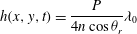 $$\begin{eqnarray}h(x,y,t)=\frac{P}{4n\cos {\it\theta}_{r}}{\it\lambda}_{0}\end{eqnarray}$$
with
 $P=2p+1$
and
 $P=2p$
for constructive and destructive interferences respectively,
 $p$
the fringe order,
 $n$
the refractive index of the foaming solution and
 ${\it\theta}_{r}$
the refraction angle (verifying
 $\sin {\it\theta}_{i}=n\,\text{sin}\,{\it\theta}_{r}$
). To measure the absolute value of the thickness, images are recorded until the appearance of a common black film. As only extrema of the light intensity are recorded, the incertitude of the measurements is given by
 $1/8$
of the light wavelength, i.e. 60 nm. The spatial incertitude is also
 $1/4$
of the distance between two extrema. A comparison between the two methods carried on experiments with the same parameters shows a good agreement, which confirms the validity of our experimental investigation, as reported in figure 2(e,f).
2.4. Surfactant solutions
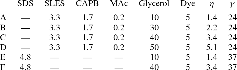
To probe the effect of surface properties and surfactant types, different foaming solutions are used in the experiments, whose compositions are presented in table 1. The first class of surfactant solutions consists in a mixture of an anionic surfactant sodium lauryldioxyethylene sulfate (SLES, product of Stepan Co., Northfield, IL; commercial name STEOL CS-170), and a zwitterionic surfactant cocoamidopropyl betaine (CAPB, product of Goldschmidt, Essen, Germany; commercial name Tego Betaine F50), with the addition of myristic acid (MAc, Fluka, purum g 98.0 GC, Cat. No. 70082), known to have a high surface dilatational modulus, and thus to entail rigidity to liquid-gas interfaces (Golemanov et al. Reference Golemanov, Denkov, Tcholakova, Vethamuthu and Lips2008). The second class of surfactant solution contains an anionic surfactant, sodium dodecyl sulfate (SDS, Sigma, 98.5 %, No. L4509) with various glycerol contents to vary the bulk viscosity.
Solutions compositions and properties: concentration of SDS, SLES, CAPB, and MAc (
 $\text{g}~\text{l}^{-1}$
), glycerol content (wt%), dye content (
 $\text{g}~\text{l}^{-1}$
), viscosity
 ${\it\eta}$
(mPa s) and surface tension
 ${\it\gamma}$
(
 $\text{mN m}^{-1}$
) at room temperature (
 ${\sim}23\,^{\circ }\text{C}$
).
3. Experimental results
The liquid dynamics inside the freshly formed film has been studied for the different surfactant solutions reported in table 1, and two behaviours are observed, as depicted in figure 3.
The first is observed in experiments performed with solutions A–D (table 1). The velocity
 $V(x,y=0,t)$
of the liquid in the film along the
 $x$
-axis normalized by the velocity of the surrounding Plateau borders
 $V_{PB}(t)=\dot{L}(t)$
is reported in figure 3(a). The origin of time is taken when the vertex is symmetrical (see figure 1). Inside the film, the velocity is constant and equal to zero (within error bars) on 80 % of the film length. The zone near the Plateau border region cannot be probed (because of internal reflexions due to interface curvature preventing light collection), but velocity variations in this zone are expected. If this profile is fitted by a linear relation, the resulting slope is equal to
 $0.1\pm 0.1$
, whatever the time at which it is taken, as shown in figure 3(d). The thickness profile of the film is measured by interferometry, thicknesses reported varying between 100 and 500 nm, as shown in figure 3(g). It shows a maximum in the middle of the film and a minimum near the surrounding Plateau borders, both decreasing when the film length increases.
The second behaviour is observed with solutions E and F (differing only by their glycerol content). The normalized velocity profiles are represented in figure 3(b,c) for viscosities of 1.4 and 3.4 mPa s respectively, at a time
 $t=10~\text{ms}$
. They both show a linear dependency up to
 $0.8x/L(t)$
. However, the velocity profiles have slopes
 $k$
equal to
 $0.45\pm 0.2$
and
 $0.75\pm 0.2$
for bulk viscosities of 1.4 and 3.4 mPa s, respectively (figure 3
e,f). A homogeneous extension of the film would lead to
 $k=1$
. Moreover, the slope of the velocity profile is constant with time for the lower viscosity, while it increases for higher viscosities. Thickness profiles, measured by absorption, show in figure 3(h,i) a thinning of the entire film during its extension. At a given time, the thickness is maximal in the middle of the film, and presents a minimum close to the surrounding Plateau borders. However, the profile is rounded for the lower viscosity, and almost flat for the higher one. The thickness of the film is of the order of several micrometers, compared with hundreds of nanometers for solution A–D.
(a–c) Velocity
 $V$
of the particles normalized by the velocity of the Plateau border
 $V_{PB}$
, as a function of the position normalized by half of the length of the film
 $L$
at time
 $t=380~\text{ms}$
(a), or at time
 $t=10~\text{ms}$
(b,c). All of the data are measured along the
 $x$
-axis. (d–f) Evolution of the slope of the normalized velocity profile, calculated as the mean along the
 $x$
- and
 $y$
-directions, with time. (g–i) Thickness profiles of the liquid film during the rearrangement. (a–d) are obtained for solutions A (first column); (b–e) and (c–f) for solutions E and F, respectively (viscosities of 1.4 and 3.4 mPa s). These results are obtained with
 $R_{c}=280~{\rm\mu}\text{m}$
. (a,d,g) Solution A, large interfacial rigidity
 ${\it\eta}=1.4~\text{mPa}~\text{s}$
. (b,e,h) Solution E, low interfacial rigidity
 ${\it\eta}=1.4~\text{mPa}~\text{s}$
. (c,f,i) Solution F, low interfacial rigidity
 ${\it\eta}=3.4~\text{mPa}~\text{s}$
.

The timescale of the topological rearrangement is also different for the two cases because of the variations of the relaxation duration. All the results are presented for the frame of side 8 mm. Similar results for the two other frames have been observed.
To summarize, the observations can be rationalized by considering two limiting cases.
-
(a) The first one concerns rigid interfaces, for which the formation of the new film is made possible by the extraction of liquid from the Plateau borders, acting as reservoirs during their movement. Indeed, the liquid inside the new film is initially in the Plateau borders, and stays at rest after its creation. It corresponds to
 $k=0$
. This process of film pulling from the Plateau border is sketched in figure 4(a), and has been proposed before (Buzza, Lu & Cates Reference Buzza, Lu and Cates1995; Biance et al.
Reference Biance, Delbos and Pitois2011; Seiwert et al.
Reference Seiwert, Monloubou, Dollet and Cantat2013). It corresponds fairly to the case experimentally observed in figure 3(d), with
$k=0.1$
.
-
(b) In the case of highly mobile interfaces, the film is stretched and has no interaction with the Plateau borders. The flow is purely elongational, and the slope of the velocity profile is
$k=1$
. The results observed in figure 3(f) with
$k=0.75$
corresponds approximately to this second case.


Between these two cases, figure 3(e) shows an intermediate slope near 0.5 (
 $k=0.45$
), which suggests a competition between the two mechanisms. In the next section, these behaviours are studied in more details.
Two limit cases of film formation, with the state at
 $t$
represented on the left, and the state at
 $t+\text{d}t$
represented on the right. The colour indicates different volumes of fluid, followed during their deformation and motion. (a) Pulling: the thin film at
 $t$
(in grey) is not deformed and some of the fluid present in the Plateau border at
 $t$
goes into the film at
 $t+\text{d}t$
. The velocity in the thin film is 0, so
 $k=0$
. (b) Stretching: there is no volume exchange between the film and the Plateau border. The thin film of length
 $2L$
at
 $t$
(in grey) is stretched at
 $t+\text{d}t$
to reached the length
 $2L+2\dot{L}\text{d}t$
. The velocity in the film is
 $V_{x}=\dot{L}x/L$
, corresponding to
 $k=1$
. Actual deformation is a combination of these two limit cases, leading to
 $0\leqslant k\leqslant 1$
.

4. Discussion
4.1. Stretching or pulling: dimensional analysis
We observed two mechanisms of film formation during topological rearrangements. The first consists of the pulling of the film from the Plateau border whereas the second is an elongation of the film. In our experiments, both effects contribute as we do not recover a purely elongation velocity profile in the case of mobile interfaces and a strictly zero velocity profile in the case of rigid interfaces. The relative contribution of these two mechanisms can be estimated from mechanical bulk and interfacial rheological properties by scaling laws, considering that the less-dissipative mechanism of extension will be selected. Stretching is associated with surface elongation and therefore dissipation by surface viscosity whereas pulling is associated with shear and bulk viscous dissipation. Whereas the driving force for T1 relaxation process is mainly surface tension (
 $f\sim {\it\gamma}$
) up to geometrical factors, the drag force (per unit length) associated to surface elongation is mainly related to the surface viscosity
 ${\it\eta}_{s}^{\ast }$
(Durand & Stone Reference Durand and Stone2006; Biance et al.
Reference Biance, Cohen-Addad and Hohler2009):
 $f_{e}\sim {\it\eta}_{s}^{\ast }\dot{L}/L$
. The drag force associated to film pulling reads
 $f_{p}\sim {\it\gamma}({\it\eta}\dot{L}/{\it\gamma})^{2/3}$
(Cantat Reference Cantat2013). Both contributions are of the same order of magnitude when the length of the film is
 $L_{c}\sim {\it\eta}_{s}^{\ast }/{\it\eta}$
, which is in fact the Boussinesq length. For
 $L<L_{c}$
, pulling is dominant as for
 $L>L_{c}$
, stretching contribution is larger. This scaling analysis underlines different points and captures qualitatively our observations.
-
(a) When surface viscosity is dominant, stretching dissipation becomes larger than pulling dissipation, and this last mechanism of film formation is selected, as observed in the case of rigid interfaces.
-
(b) When bulk viscosity is dominant, stretching of the film will be more favourable as observed for the more viscous films where the elongation process is more robust.
-
(c) During the process, as
$L$
is increasing, the ratio of both contributions varies, the pulling being predominant for small
$L$
(short times) then replaced by elongation as the film grows in size. Thus, the slope of the velocity profile is expected to increase with time, as observed in figure 3(f).


One can note that this sequence of events (pulling followed by extensional flow) differs with experiments reported recently on the elongation of an already formed soap film on a frame (Seiwert et al.
Reference Seiwert, Monloubou, Dollet and Cantat2013), where an extensional flow, attributed to Marangoni stress establishment, is followed by a pulling mechanism. However, in this case, the film is stretched from an already formed film with a non-negligible size
 $L$
at a prescribed rate. These different initial conditions are crucial to understanding the physical mechanism at stake during the film generation. Indeed, to ensure pulling of a Frankel’s film, an interfacial stress gradient (a Marangoni stress) must be established at the film surface to balance bulk viscous stresses (Cantat Reference Cantat2013). This necessary stress is very low and can have different origins. One of them, an inhomogeneous repartition of surfactants on the film surface, requires a small extension (
 $L/L_{0}$
) of the film at the beginning of the process of less than 1 % (Seiwert et al.
Reference Seiwert, Monloubou, Dollet and Cantat2013). In the case of a topological relaxation, the initial size
 $L_{0}$
of the film is very small and this critical elongation is instantaneously reached during the vertex dissociation, and cannot be captured experimentally. Then, the pulling mechanism is established, until surface elongation requires less dissipation, i.e. when the elongation rate is decreased (lower velocity, larger films). During this last step of film elongation, rheological properties of the interface due to so-called Marangoni effects must be taken into account. For simplicity, the effect of surface elasticity has been neglected as only a dependency of the stress with elongation rate, through surface viscosity, has been taken into account. A careful study of full interfacial rheological properties would be needed to conclude on this point, which is not in the scope of this study.
4.2. Pulling: the case of liquid extracted from Plateau borders
In the case of solutions A–D (table 1), film generation and film thickness profile are mainly governed by exchange between the film and its adjacent meniscus (PB). In this type of exchange, the film thickness is given by a balance between capillary suction and viscous entrainment, as in the common well-known Frankel’s situation (Mysels & Frankel Reference Mysels and Frankel1978) of a film withdrawn at constant velocity from a bath. The thickness of the entrained film is predicted to linearly depend on the radius of curvature of the meniscus and to depend on the entrainment velocity through a capillary number
 $h\sim R_{c}\mathit{Ca}^{2/3}$
. Similarly to this approach, we plot in figure 5 the local minimal thickness normalized by the radius of curvature of the Plateau border, participating to capillary suction, versus the instantaneous capillary number based on Plateau border velocity measured through
 $L$
(
 $\mathit{Ca}={\it\eta}\dot{L}/{\it\gamma}$
). We performed the experiments for different liquid viscosities and different radii of curvature of the Plateau border. All of the curves appear to collapse on a master curve, the thickness of the film being in good agreement with the capillary number at the power
 $2/3$
. However, the obtained prefactor is
 $4.5\pm 1.2$
, whereas the value predicted by Frankel’s theory is 2.68. This discrepancy can be attributed to several factors.
(a) Minimal thickness of the film normalized by the radius of curvature of the Plateau border, as a function of the capillary number
 $\mathit{Ca}={\it\eta}V/{\it\gamma}$
. The curve gather measurements for the frame of side
 $8~\text{mm}$
with
 ${\it\eta}=1.4~\text{mPa s}$
and
 $240<R_{c}<320~{\rm\mu}\text{m}$
(
 $\times$
),
 ${\it\eta}=1.4~\text{mPa s}$
and
 $160<R_{c}<240~{\rm\mu}\text{m}$
(▵),
 ${\it\eta}=1.4~\text{mPa s}$
and
 $110<R_{c}<160~{\rm\mu}\text{m}$
(
 $\star$
),
 ${\it\eta}=2.2~\text{mPa s}$
and
 $240<R_{c}<320~{\rm\mu}\text{m}$
(*),
 ${\it\eta}=2.2~\text{mPa s}$
and
 $110<R_{c}<160~{\rm\mu}\text{m}$
(
 $+$
),
 ${\it\eta}=3.4~\text{mPa s}$
and
 $240<R_{c}<320~{\rm\mu}\text{m}$
(▫),
 ${\it\eta}=5.1~\text{mPa s}$
and
 $240<R_{c}<320~{\rm\mu}\text{m}$
(▿), and for the frame of side 4 mm with
 ${\it\eta}=1.4~\text{mPa s}$
(○). The dashed line corresponds to Frankel’s law
 $h/R_{c}=2.68\mathit{Ca}^{2/3}$
and the straight line corresponds to a fit of the data with
 $h/R_{c}=4.5\mathit{Ca}^{2/3}$
. (b) Scheme representing Plateau border radius of curvature variations due to out-of-equilibrium shape of film assembly, the angle varying between
 ${\rm\pi}/2$
at the beginning of the relaxation process to
 $2{\rm\pi}/3$
.

4.2.1. Steady-state approximation and finite size of the film
Frankel’s law describes the pulling of an infinite flat film at a constant velocity. The assumptions rely on steady-state approximation, stating that the velocity is not varying with time and that the pulled film is flat far from the meniscus. In our cases, velocity variations indeed induce film thickness variations and this steady-state approximation can be discussed. Low Reynolds number (
 $\mathit{Re}<1$
) and slender slope approximation (
 $\partial h/\partial x\ll 1/100$
) allow us to use Stokes equation and to recover unsteady-state thin-film equation evolution (Cormier et al.
Reference Cormier, McGraw, Salez, Raphael and Dalnoki-Veress2012; Seiwert et al.
Reference Seiwert, Monloubou, Dollet and Cantat2013), described below (4.5).
Unsteady effect could thus be a priori non-negligible. However, comparing the experimental data to the unsteady solution obtained by the numerical resolution of (4.5) does not lead to a better agreement, thus excluding such possibility.
4.2.2. Out-of-equilibrium Plateau border shape and radius of curvature
During the topological rearrangement, the Plateau border is out of equilibrium and its shape can be therefore distorted, as depicted in figure 5(b). This shape distortion should result in a variation of Plateau border radius of curvature. A simple geometric analysis shows that for angles of the two adjacent films varying between
 ${\rm\pi}/2$
and
 $2{\rm\pi}/3$
, the radius of curvature can increase up to 40 %. Taking this effect into account, the discrepancy with Frankel’s law is a factor of about 1.4, instead of the factor of 1.8 obtained from our experimental observations.
4.3. Elongation of the film
4.3.1. Self-similarity
To check that particles act as passive tracers and that the velocity profile proposed is valid, we test volume conservation through self-similarity in the elongated part of the film. Because the interference pattern appears circular (figure 2
d), the analysis proposed in the following is performed in axisymmetric geometry. A direct comparison of the radial velocity
 $V$
obtained in the modelling will be performed with experimental velocity
 $V$
measured on the
 $x$
-axis. For the two experiments with solutions E and F (table 1), the flow is assumed to be almost plug like within the film, and the velocity to follow a partial elongational profile as observed before:
 $$\begin{eqnarray}V(r,t)=k\frac{r}{L(t)}\frac{\partial L(t)}{\partial t}\end{eqnarray}$$
where
 $k$
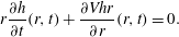
is the slope of the velocity profile. The 2D liquid volume conservation within the film implies, assuming an axisymmetric film:
 $$\begin{eqnarray}r\frac{\partial h}{\partial t}(r,t)+\frac{\partial Vhr}{\partial r}(r,t)=0.\end{eqnarray}$$
The combination of (4.1) and (4.2) gives
 $$\begin{eqnarray}\frac{\partial h}{\partial t}(r,t)=-k\frac{\dot{L}(t)}{L(t)}\left(2h(r,t)+r\frac{\partial h}{\partial r}(r,t)\right).\end{eqnarray}$$
One solution satisfying this equation reads
 $$\begin{eqnarray}h(r,t)=\frac{1}{L(t)^{2k}}\,f\left(\frac{r}{L(t)^{k}}\right).\end{eqnarray}$$
The function
 $f$
is an arbitrary function, which is the shape of the film conserved during the elongation.
(a,b) Self-similarity of thickness profiles measured by absorption for solutions of SDS and dye at viscosities of 1.4 (a) and 3.4 mPa s (b) with
 $R_{c}=280~{\rm\mu}\text{m}$
(from figure 3
h,i). Here
 $k$
is adjusted to superimpose the thickness profiles, and is here equal to 0.36 and 0.95 for 1.4 and 3.4 mPa s, respectively.

The thickness profiles, multiplied by
 $L(t)^{2k}$
, taken at different times, are represented as a function of
 $x/L(t)^{k}$
in figure 6(a) for a viscosity of 1.4 mPa s. It shows a good self-similarity between the thickness profiles, which confirms that particles follow the liquid flow inside the film. The value of
 $k$
used to adjust the profiles is
 $0.36\pm 0.06$
for a viscosity of 1.4 mPa s. A shown in figure 6(b), results are similar for a higher viscosity of 3.4 mPa s, as we observe again a self-similarity with a factor
 $k=0.95\pm 0.25$
for times higher than 10 ms. However, the first profiles do not superimpose, which is attributed to the increase of the slope of the velocity profile with time for the higher viscosity, as represented in figure 3( f). For the two viscosities, the factors
 $k=0.36$
and
 $k=0.95$
are compatible with the slope of the velocity profiles obtained on figure 3(b,c),
 $k=0.45$
and
 $k=0.75$
, respectively. It allows us to verify the volume conservation and thus the validity of the velocity profiles measured.
Moreover, the thickness profiles shown in figure 6 exclude the
 $100~{\rm\mu}\text{m}$
adjoining the meniscus. In fact, the profile wings do not superimpose through the law of volume conservation, which is consistent with a slope of the velocity profile lower than 1 and liquid exchange between the Plateau borders and the film.
4.3.2. Limitation of the self-similarity
At the beginning of the T1, when the film is not created yet, the shape of the liquid meniscus at the eight-fold vertex point is almost circular and at first order well described by a parabolic shape. The minimal thickness of liquid is observed in the middle of the vertex at
 $r=0$
. Then during the film formation process, a bump in the middle of the film appears, reminiscent to dimples observed during film drainage (Chan, Klaseboer & Manica Reference Chan, Klaseboer and Manica2010). The thickness becomes maximal in the middle of the film and minimal near the Plateau borders (see figure 3
h), so the curvature of the liquid interfaces at the point
 $r=0$
is positive initially and negative at later times. Moreover, the profiles obtained at the two different viscosities do not have the same shape, the higher viscosity corresponding to a flatter profile. The curvature inversion occurs at early time and is not visible on figure 6. It cannot be predicted with the elongational model discussed in § 4.3, as it does not respect the self-similarity associated with this simple model. Moreover, the elongational model of § 4.3 does not predict nor explain the value of the parameter
 $k$
, which is an adjustable parameter of this first approach. In the case of the higher viscosity (3.4 mPa s), the slope of the velocity profile is near 1, which is the expected value for a purely extensional process (see figure 4). However, in the case of the lower viscosity (1.3 mPa s), the slope of the velocity profile is near 0.5 and the contribution of the pulling process can no longer be neglected. In the complex dynamics involving both processes the central part of the film is elongated and the shape is thus self-similar, but new film is extracted from the Plateau border, with a thinner thickness. This is consistent with the observation made on figure 6(a): the central part is self-similar, but the film length, even in rescaled units, increases with time. The value of
 $k$
, the curvature inversion at short time, and more generally the prediction of the whole film shape are not captured by the simple elongation model discussed in 4.3 and required a more detailed modelling proposed in the following.
4.4. Combination of the two mechanisms
4.4.1. Unsteady lubrication model
The Frankel’s theory assumes an infinite viscosity at the interface (or equivalently an infinite Gibbs elasticity), that is Marangoni effects which are so strong that the interfacial extension is of negligible amplitude; this leads to the prediction used in § 4.2 for the film thickness. In contrast the stretching case proposed in § 4.3 is only possible if the interfacial stress is negligible. In order to combine these two limiting cases in a more complete theory, we need to take into account the interfacial rheology. Both the viscous and elastic properties of the film should in principle be considered. For sake of simplicity, we only consider viscous aspect here. We thus define the surface viscosity
 ${\it\eta}_{s}^{\ast }={\it\eta}_{s}+{\it\kappa}_{s}$
, with
 ${\it\eta}_{s}$
the shear interface viscosity and
 ${\it\kappa}_{s}$
the dilatational interface viscosity.
The time evolution of the film is obtained from the lubrication equations, which take into account the capillary suction of the meniscus and the Marangoni flow induced by the interfacial stress gradients. Two equations, detailed in appendix A, govern the coupling between the interfacial velocity
 $v_{s}$
and the film thickness
 $h(r,t)$
, in axisymmetric geometry:
 $$\begin{eqnarray}h_{t}=-\frac{1}{r}\partial _{r}\left[\frac{{\it\gamma}}{3{\it\eta}}rh^{3}\left(h_{rrr}+\partial _{r}\left(\frac{h_{r}}{r}\right)\right)+rv_{s}h\right]\end{eqnarray}$$
where the surface velocity is set by stress balance at the interface (see appendix A):
 $$\begin{eqnarray}v_{s,rr}+\partial _{r}\left(\frac{v_{s}}{r}\right)=-\frac{{\it\gamma}}{{\it\eta}_{s}^{\ast }}h\left(h_{rrr}+\partial _{r}\left(\frac{h_{r}}{r}\right)\right).\end{eqnarray}$$
These equations require different boundary conditions. The solution must match asymptotically a static meniscus with a constant given mean curvature
 $c_{0}=1/R_{c}$
whose profile is described by:
 $$\begin{eqnarray}h_{asymptotic}=h_{l}+\frac{c_{0}r_{0}(t)^{2}}{2}\ln \left(\frac{r}{r_{l}}\right)+\frac{c_{0}}{4}(r^{2}-r_{l}^{2}).\end{eqnarray}$$
This shape reaches a minimum value at
 $r=r_{0}(t)$
and its mean curvature is
 $c_{0}$
everywhere. Here
 $r_{l}$
is an arbitrary reference point, and the thickness at this point is
 $h_{l}$
. This point
 $r_{l}$
will be chosen much larger than
 $r_{0}$
and will be used as the matching point between the dynamical solution determined numerically and the static meniscus. The experimental velocity of the meniscus is taken into account in the simulation to impose the boundary condition at
 $r=r_{l}$
. Indeed, the value of
 $r_{0}$
is modified at each time step according to this experimental velocity, and the thickness derivatives at
 $r=r_{l}$
are obtained with (4.7). Symmetry conditions are applied at
 $r=0$
. The initial thickness profile
 $h(r,0)$
is calculated from an initial experimental thickness profile
 $h_{exp}(x,0)$
. The only adjustable parameter is the dimensionless parameter
 ${\it\lambda}=(3{\it\eta}R_{c})/{\it\eta}_{s}^{\ast }$
. The numerical resolution of (4.5) and (4.6) is performed using a standard implicit method as in Kondic (Reference Kondic2003).
4.4.2. Comparison with experimental results
A comparison between the experimental and integrated profiles is shown in figure 7(a) for the lower viscosity, and in figure 7(d) for the higher viscosity. The initial profile is the initial condition for the simulation. In both cases, the same value of
 ${\it\lambda}$
is kept at all time steps and allows the profile evolution to be captured.
(a–d) Experimental thickness profiles (continuous lines) compared with simulated thickness profiles obtained from integration of (4.5) and (4.6) (dashed lines). The light dashed line is the initial profile for the simulation, calculated from the corresponding experimental profile as a continuous trace. Thicknesses are reported in dimensionless units
 $H=h/(R_{c}(3Ca)^{2/3})$
, as a function of the dimensionless position
 $X=x/(R_{c}(3Ca)^{1/3})$
. (b–e) Experimental thickness in the middle of the film as a function of the simulated central thickness, corresponding to
 $X=0$
on figures (a,d). (c–f) Experimental minimal thickness as a function of the minimal thickness obtained with our simulation (o), and as a function of the Frankel’s prediction (♢). The measurements (a–c) correspond to the low viscous case (1.3 mPa s) with a radius of curvature of
 $250~{\rm\mu}\text{m}$
and
 ${\it\lambda}=0.02$
, and (d–f) to the high viscous case (3.4 mPa s) with a radius of curvature of
 $224~{\rm\mu}\text{m}$
and
 ${\it\lambda}=0.07$
. Lines correspond to a linear fit, whose slopes are close to one (0.97, 1.14, 0.98 and 1.13 for (b,c,e,f) respectively). Results are obtained for solution F (top line) and G (bottom line).

Indeed, the evolution of the experimental thickness is represented as a function of the integrated thickness in the middle
 $h^{mid}$
(figure 7
b,e) and at the border of the film
 $h^{min}$
(figure 7
c, f): the relations are almost linear, with slopes close to 1. The comparison of
 $h^{min}$
with the thickness predicted by the Frankel’s law highlights the unsteady property of the T1 dynamics, whereas the introduction of
 ${\it\lambda}$
in simulations and the variations of the middle thickness with time highlights the elongation of the film.
The values obtained for the parameter
 ${\it\lambda}$
are
 $0.025\pm 0.005$
and
 $0.07\pm 0.005$
for viscosities of 1.3 and 3.4 mPa s, respectively, which corresponds to surface viscosities of
 $0.08\pm 0.04$
and
 $0.04\pm 0.03~\text{mPa m s}$
. These measurements are 10 times smaller than values reported in the literature (Liu & Duncan Reference Liu and Duncan2003). Discrepancies can be attributed to the presence of the dye in the solution or to the non-Newtonian properties of the interfaces, probed at larger deformation rate and shorter timescales than usually.
5. Conclusion
These new experiments underline that film generation during a topological rearrangement is a complex process. Depending on the nature of the surfactants used, and therefore on the rheological properties of the liquid and interfaces, different mechanisms of film formation are found. For very dissipative interfaces, a pulling mechanism from the adjacent Plateau border is observed, the film nourished throughout the extraction process. In contrast, for almost stress-free interfaces, a self-similar elongation and subsequent thinning of the central film is observed, connection with Plateau borders taking place only on the edge of the films. By numerically solving unsteady thin-film equation, the film profile can be recovered and therefore the surface viscosity of the interfaces can be deduced. These results underly that a general mode of dissipation during a T1 process is not valid, and are a new starting point for T1 dynamic studies in these various cases, as well as for defining conditions for film rupture during these dynamical events (Carrier & Colin Reference Carrier and Colin2003; Biance et al. Reference Biance, Delbos and Pitois2011).
Acknowledgements
This project has been funded by CNES through convention CNRS/CNES number 127233 and by Région Rhone Alpes through ARC contract 13-010053-01. J.S. acknowledges financial support from Région Bretagne (CREATE MOUSPORE) and Agence Nationale de la Recherche (ANR-13-PDOC-0014-01-HYDROSURFDYN).
Appendix A
This appendix establishes the set of coupled partial differential equations governing the time evolution of the film thickness
 $h(r,t)$
and of the interfacial velocity
 $v_{s}(r,t)$
. The radial velocity in the film
 $v(r,z,t)$
is governed by the lubrication equations in an axisymmetric geometry. The pressure
 $P(r,t)$
only depends on the radial coordinate
 $r$
and is fixed by the Laplace pressure jump at the interface. In the following, the subscript
 $r$
,
 $z$
or
 $t$
denotes a partial derivative with respect to the corresponding variable.
 $$\begin{eqnarray}P=-{\it\gamma}\left(h_{rr}+\frac{h_{r}}{r}\right).\end{eqnarray}$$
The Stokes equation
 $P_{r}={\it\eta}v_{zz}$
is integrated three times with respect of the transverse coordinate
 $z$
to compute the radial flux
 $Q$
at the position
 $r$
:
 $$\begin{eqnarray}Q=2{\rm\pi}r\frac{{\it\gamma}}{3{\it\eta}}h^{3}\left(h_{rrr}+\partial _{r}\left(\frac{h_{r}}{r}\right)\right)+2{\rm\pi}rhv_{s}.\end{eqnarray}$$
The integration constants are given by the symmetry conditions
 $v_{r}(r,0)=0$
and by the relation
 $v(r,h)=v_{s}(r)$
.
The mass conservation imposes
 $$\begin{eqnarray}h_{t}=-\frac{1}{r}\partial _{r}\left[\frac{{\it\gamma}}{3{\it\eta}}rh^{3}\left(h_{rrr}+\partial _{r}\left(\frac{h_{r}}{r}\right)\right)+rv_{s}h\right].\end{eqnarray}$$
The problem is closed with the Marangoni relation, i.e. the condition of tangential stress continuity at the interface:
 $$\begin{eqnarray}{\it\eta}v_{z}(r,h)={\it\eta}_{s}^{\ast }\left(v_{s,rr}+\partial _{r}\left(\frac{v_{s}}{r}\right)\right)\end{eqnarray}$$
which leads to
 $$\begin{eqnarray}v_{s,rr}+\partial _{r}\left(\frac{v_{s}}{r}\right)=-\frac{{\it\gamma}}{{\it\eta}_{s}^{\ast }}h\left(h_{rrr}+\partial _{r}\left(\frac{h_{r}}{r}\right)\right).\end{eqnarray}$$
Equations (A 3) and (A 5) are solved numerically, with appropriate conditions at
 $t=0$
,
 $r=0$
and
 $r\rightarrow \infty$
, as discussed in the text.



