1 Introduction
Parallel-in-time methods aim to pararallelize the time simulation of initial-value problems over the time domain. In the Parareal algorithm, first proposed by Lions et al. [Reference Lions, Maday and Turinici9], a fine time-propagator (accurate but with long wall-clock time) is applied on small chunks of the time domain in parallel. A correction is provided by a coarse time-propagator (which is fast but with reduced accuracy) that is applied sequentially over the complete time domain.
More specifically, let
 $u(t): \mathbb R \rightarrow \mathbb R^d$
be a function of time t, let
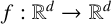 $f :\mathbb R^d \rightarrow \mathbb R^d$
be a function and
 $\alpha \in \mathbb R^d$
be a constant vector, then the Parareal method applies to ordinary differential equation (ODE) problems of the form
 $$ \begin{align} du/dt = f(u), \quad u(0) = \alpha \end{align} $$
on a time interval
 $[0, \, T]$
. The time domain is divided in N subintervals of equal length
 $\Delta t = T/N$
, and points on the time grid are denoted with
 $t_n = n \Delta t$
for
 $0 \leq n \leq N$
. Let
 $\mathcal F$
be a fine solver,
 $\mathcal F: \mathbb R^d \rightarrow \mathbb R^d$
, numerically evolving an approximate solution to equation (1.1) over a chunk of time
 $\Delta t$
, and similarly let
 $\mathcal C: \mathbb R^d \rightarrow \mathbb R^d$
be a coarse solver.
The Parareal iterate
 $u^k_n$
with index
 $k \geq 0$
for iteration number and with time index n for
 $0 \leq n \leq N-1$
, obeys the double recursion:
 $$ \begin{align*} \begin{cases} u^{k}_{n+1} = \mathcal C (u^{k}_{n}), & k=0, \\ u^{k+1}_{n+1} = \mathcal F(u^{k}_{n}) + \mathcal C( u^{k+1}_{n}) - \mathcal C(u^{k}_{n}), & k> 0. \end{cases} \end{align*} $$
Typically, a reference solution
 $u_n$
is defined as the result of the sequential application of the fine solver:
 $u_0 = \alpha $
and
 $u_{n+1} = \mathcal F(u_n)$
for
 $0 \leq n \leq N-1$
. The approximations by the Parareal algorithm then possesses a finite-termination property, namely
 $u^k_n = u_n$
for
 $k \geq n$
(see [Reference Gander and Vandewalle6, Theorem 3.1 and Remark 4.7]). In practice, Parareal is also applicable for nonautonomous problems and nonuniform time grids.
The convergence of Parareal for linear scalar differential equations is given by the following theorem by [Reference Gander and Vandewalle6, Corollary 4.6 and Theorem 4.9].
Lemma 1.1. Let
 $\mathcal F(u) = fu$
be a scalar fine propagator and
 $\mathcal C(u) = gu$
be a scalar coarse propagator with
 $f,g \in \mathbb R$
and
 $|g|< 1$
. Then, the maximum error,
 ${E^{k}_{\mathrm \max } = \max _{1\leq n \leq N} |u^k_n - u_n|}$
, satisfies a superlinear bound
 $$ \begin{align} E^{k}_{\mathrm\max} \leq | f-g |^k \binom{N-1}{k} E^{0}_{\mathrm\max} \end{align} $$
and a linear bound
 $$ \begin{align} E^{k}_{\mathrm\max} \leq \bigg( \frac{| f-g |}{1-| g |} \bigg)^k E^{0}_{\mathrm\max}. \end{align} $$
In micro-macro Parareal, which is a generalization of Parareal, the coarse propagator does not act on the original state variable
 $u \in \mathbb R^d$
(micro state), but instead on a reduced version
 $U \in \mathbb R^r$
(macro state). These micro and macro states are coupled. A restriction operator
 $\mathcal R: \mathbb R^d \rightarrow \mathbb R^r$
extracts macro information from a micro state. A lifting operator
 $\mathcal L$
provides a unique micro state u, consistent with a given macro state U. That is,
 $\mathcal {L}: \mathbb R^r \rightarrow \mathbb R^d: u = \mathcal L(U)$
such that
 $\mathcal R(u) = U$
.
Blouza et al. [Reference Blouza, Boudin and Kaber2] proposed one possible micro-macro Parareal algorithm (see also Legoll et al. [Reference Legoll, Lelièvre and Samaey8, equation (3.21)]). The micro initial condition for all iterations k is
 $u^k_0 = u_0$
and the macro initial condition equals
 $U^k_0 = \mathcal R (u_0)$
. In the zeroth iteration, one computes
 $U^0_{n}$
and
 $u^0_{n}$
sequentially for
 $n=1 \cdots N$
as
 $$ \begin{align} \begin{aligned} U_{n+1}^{0} &= \mathcal{C} (U_n^{0}), \\ u_{n+1}^{0} &= \mathcal{L}(U_{n+1}^{0}). \end{aligned} \end{align} $$
In the subsequent iterations,
 $$ \begin{align} \begin{aligned} u_{n+1}^{k+1} &= \mathcal{F} (u_n^k)+\mathcal L [ \mathcal{C} (\mathcal{R} (u_n^{k+1}) ) - \mathcal{C}( \mathcal{R} ( u_n^k) ) ], \\ U^{k+1}_{n+1} &= \mathcal R (u^{k+1}_{n+1}). \end{aligned} \end{align} $$
Depending on the context, however, a lifting operator may involve costly computations. In that case, a matching operator can be used instead. A matching operator
 $\mathcal M$
outputs a micro state u consistent with a given macro state U, based on prior information about the micro state
 $\hat u$
, that is,
 $\mathcal M: (\mathbb R^r ,\, \mathbb R^d) \rightarrow \mathbb R^d: \mathcal M(U, \hat u) = u$
such that
 $\mathcal R(u) = U$
.
Another micro-macro Parareal algorithm, using a matching operator, was proposed by Legoll et al. [Reference Legoll, Lelièvre and Samaey8, Algorithm 2]. As in the previous algorithm, the micro initial condition for all iterations k is
 $u^k_0 = u_0$
and the macro initial condition equals
 ${U^k_0 = \mathcal R (u_0)}$
. It starts with equation (1.4), and replaces equation (1.5) by
 $$ \begin{align} \begin{aligned} U_{n+1}^{k+1} &= \mathcal{C} (U_n^{k+1}) + \mathcal{R} ( \mathcal{F} (u_n^k)) - \mathcal{C}( U_n^k), \\ u_{n+1}^{k+1} &= \mathcal{M}(U_{n+1}^{k+1}, \mathcal{F} (u_n^k)). \end{aligned} \end{align} $$
When we refer to micro-macro Parareal in the rest of this text, we refer to this variant.
Remark 1.2 (Micro and macro error).
In the study of convergence properties of the micro-macro Parareal algorithm, one may be interested in the error on the micro variable
 $u_n^k$
or in the error on the macro variable
 $U_{n}^k$
. We denote these errors
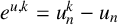 $e^{u,k} = u_{n}^k - u_n$
and
 $e^{U,k} := U_{n}^k - U_n = U^k_n - \mathcal {R}(u^k_n)$
, respectively. In practice, this choice is influenced by the context (see also Remark 2.5).
Property 1. If
 $\mathcal R$
and
 $\mathcal M$
are chosen such that for any U and u,
 $\mathcal R (\mathcal M(U, u)) = U$
, then the following properties of micro-macro Parareal equations (1.4)–(1.6) hold.
-
(i) A micro-macro consistency property, that is,
 $U^k_n = \mathcal R (u^k_n)$
for all
$n,k \geq 0$
(see [Reference Legoll, Lelièvre and Samaey8, last paragraph of Section 3.2]).
-
(ii) If, in addition,
$\mathcal M ( \mathcal R (u), u) = u$
, then a finite termination property holds:
${u^k_n = u_n}$
for all
$k \geq n$
(see [Reference Legoll, Lelièvre and Samaey8, Theorem 12]). From property (i), it also holds that
${U^k_n = U_n = \mathcal R (u_n)}$
.


Under the same assumptions of Property 1, it holds that:
-
(i)
$e^{U,k}_n = \mathcal R (e^{u,k}_n)$
for all
$n,k \geq 0$
; -
(ii)
$e^{u,k}_n = 0$
and
$e^{U,k}_n = 0$
for all
$k \geq n$
.


The rest of this paper is organized as follows. We first present a convergence bound for the micro-macro Parareal algorithm applied to a special multiscale ODE in Section 2. We present a new upper bound on the Parareal error, explicitly with respect to the iteration number. This bound is valid for a specific class of (multiscale) ODEs.
Then, in Section 3, we extend the MC-moments Parareal algorithm by Bossuyt et al. [Reference Bossuyt, Vandewalle and Samaey4], designed for the simulation of scalar (McKean–Vlasov) stochastic differential equations (SDEs) to higher dimensional SDEs. In both parts, we provide some numerical experiments to illustrate our theory and methods. The Julia implementation for all the numerical experiments is available in a public repository from [Reference Bossuyt3]. Finally, Section 4 concludes the paper.
2 Convergence theory of micro-macro Parareal for linear multiscale ODEs
In this section, we consider a two-dimensional linear multiscale ODE.
Test system and assumptions. We consider the ODE that models the evolution of a state vector
 $u = (x,y)$
, where
 $x \in \mathbb R$
is a slow variable and
 $y \in \mathbb R$
is a fast variable. It contains the parameters
 $\alpha $
,
 $\beta , \delta \in \mathbb R$
.
 $$ \begin{align} \begin{aligned} \frac{d}{dt} \left[ \begin{matrix} x \\ y \end{matrix} \right] = \left[ \begin{matrix} \alpha & \beta \\ 0 & \delta \end{matrix} \right] \left[ \begin{matrix} x \\ y \end{matrix} \right] , \quad & \left[ \begin{matrix} x(0) \\ y(0) \end{matrix} \right] = \left[ \begin{matrix} x_0 \\ y_0 \end{matrix} \right]. \end{aligned} \end{align} $$
Here, we assume that
 $\delta $
is large compared with
 $\alpha $
:
 $|\delta | \gg \alpha $
, such that the fast variable reaches its equilibrium much faster in time than the slow variable. We assume that
 $\delta < 0$
and also that
 $\delta \neq \alpha $
. This ensures that the fast variable decays to zero. If one increases the absolute value of
 $\delta $
, the numerical simulation of this system gets more expensive due to the stiffness in the y variable.
The (exact) solution to equation (2.1) equals
 $u(t+\Delta t) = \mathcal A(\Delta t) u(t)$
, where
 $$ \begin{align} \mathcal A (\Delta t) = \left[ \begin{matrix} e^{\alpha \Delta t} & (e^{\delta \Delta t} - e^{\alpha \Delta t}) \dfrac{\beta}{\delta - \alpha} \\ 0 & e^{\delta \Delta t} \end{matrix} \right]. \end{align} $$
This is a special case of the linear ODE considered by Legoll et al. [Reference Legoll, Lelièvre and Samaey8], namely, a two-dimensional case where the leftmost entry in the matrix
 $\mathcal A$
equals zero.
Reduced model. Now we build a one-dimensional reduced model, describing only the dynamics of a slow variable U (as an approximation to x). To this aim, we introduce a modified decay rate
 $\bar {\alpha } \approx \alpha $
. The evolution of the reduced variable U is given as follows:
 $$ \begin{align} \frac{dU}{dt} = \bar \alpha U , \quad U(0) = \bar{x}_0, \end{align} $$
where
 $\bar {x}_0$
is the initial condition of the reduced model. We denote the effect of a numerical time-stepper on equation (2.3) with a scalar
 $G \in \mathbb R$
as
 $G \approx e^{\alpha \Delta t}$
.
Definition 2.1 (Operators for micro-macro Parareal on linear multiscale ODEs).
Following Legoll et al. [Reference Legoll, Lelièvre and Samaey8], we choose the micro variable
 $u = ( x, \, y )$
(corresponding to the multiscale ODE in equation (2.1)) and the macro variable U (corresponding to the reduced model in equation (2.3)). Further, we choose:
-
• a fine propagator
$\mathcal F: \mathbb R^2 \rightarrow \mathbb R^2: \mathcal F(u) := \mathcal A u$
(see the stiff model in equation (2.1)); -
• a coarse propagator
$\mathcal C: \mathbb R \rightarrow \mathbb R: \mathcal C(U) := GU$
(see the reduced model in equation (2.3)); -
• a restriction operator
$ \mathcal R: \mathbb R^2 \rightarrow \mathbb R: \mathcal R ((x, \, y)) := x$
; -
• a matching operator
$ \mathcal M: (\mathbb R, \mathbb R^2) \rightarrow \mathbb R^2: \mathcal M(U, (x, \, y)) := (U, \, y)$
; -
• a lifting operator
$ \mathcal L: \mathbb R \rightarrow \mathbb R^2: \mathcal L(U) := (U, \, 0) $
.


We divide the time interval into N subintervals of equal length.
The coarse and fine solver are linear, as the ODE problem and its reduced model are linear. The above choices suffer from the issue of initial slip; for more information, see for instance [Reference Van Kampen14, Appendix A]. We postpone a discussion of this issue to Section 2.3, where we also give some numerical experiments.
Relation to existing work. Legoll et al. [Reference Legoll, Lelièvre and Samaey8] studied the convergence of micro-macro Parareal with respect to the time-scale separation between the fast and slow variable for a more general multiscale linear ODE than the ODE in equation (2.1), that is, with a bottom left term of the matrix
 $\mathcal A$
possibly different from zero. Their bound contains a constant which depends on the iteration number. That makes it difficult to predict the error of micro-macro Parareal a priori as a function of the iteration number. In this work, we wish to obtain a convergence bound directly with respect to the iteration number.
2.1 A nontight error bound
In this section, we first interpret micro-macro Parareal for the multiscale ODE as a special case of classical Parareal. We then explain why it is not possible to readily apply the convergence theory from Gander and Vandewalle [Reference Gander and Vandewalle6], because the coarse and fine propagators do not commute. Then, we derive a bound on the error of micro-macro Parareal, based on the generating functions methodology developed by Gander et al. [Reference Gander, Lunet, Ruprecht and Speck5].
Preparatory considerations.
Definition 2.2 (Introduction of symbols).
To make notation shorter, we introduce
 $F = e^{\alpha \Delta t}$
and
 $b = (e^{\delta \Delta t} - e^{\alpha \Delta t}) {\beta }/({\delta - \alpha })$
. We also define the matrix
 $\mathcal B$
as follows:
 $$ \begin{align} \mathcal B = \left[ \begin{matrix} G & 0 \\ 0 & 0 \end{matrix} \right]. \end{align} $$
We first present a lemma about the interpretation of the micro-macro Parareal iterates as iterates of classical Parareal, with proof in Appendix A.
Lemma 2.3 (Interpretation of micro-macro Parareal as classical Parareal).
The use of micro-macro Parareal equations (1.4)–(1.6) with the operators from Definition
2.1
is equivalent to the application of classical Parareal with a fine propagator
 $\mathcal F: \mathbb R^2 \rightarrow \mathbb R^2: \mathcal F(u) = \mathcal Au$
and a coarse propagator
 $\mathcal C: \mathbb R^2 \rightarrow \mathbb R^2: \mathcal C(u) = \mathcal Bu$
:
 $$ \begin{align}\begin{aligned} u^0_{n+1} &= \mathcal B u^0_n , \\ u^{k+1}_{n+1} &= (\mathcal A - \mathcal B)u^{k}_{n}+ \mathcal{B} u^{k+1}_n. \end{aligned}\end{align} $$
Lemma 2.4 (Error equation for micro-macro Parareal iterates).
Consider micro-macro Parareal, defined in equations (1.4)–(1.6), with coarse and fine time-stepping operators and coupling operators from Definition
2.1
. The error on the micro state
 $u^k_n$
in iteration k and at time point
 $t_n$
, namely
 $e^{u,k}_n = u^k_n - u_n$
, satisfies for
 $0 \leq n \leq N-1$
,
 $$ \begin{align}\begin{aligned} e^{u,0}_{n+1} &= B u^0_n - A u_n = B^nu_0 - A^n u_0 , \\ e^{u,k+1}_{n+1} &=(\mathcal A - \mathcal B)e^{u,k}_{n}+ \mathcal{B} e^{u,k+1}_n. \end{aligned}\end{align} $$
Proof. Subtracting the reference solution
 $u_n = \mathcal A^n u_0$
on both sides of equation (2.5) leads to equation (2.6).
We denote the error on the slow variable with
 $e^{x,k}_n = x^k_n - x_n$
and the error on the fast variable with
 $e^{y,k}_n = y^k_n - y_n$
.
Remark 2.5. It is, in general, not possible to derive a closed form solution to equation for the evolution of the macro error. Indeed, using the linearity of
 $\mathcal R$
,
 $$ \begin{align*} e^{U,k+1}_{n+1} = \mathcal R ( e^{u,k+1}_{n+1} ) &= \mathcal R ( (\mathcal A - \mathcal B) e^{u,k}_{n} + \mathcal{B} e^{u,k+1}_n ) \\ &= \mathcal R ( (\mathcal A - \mathcal B) e^{u,k}_{n} ) + \mathcal R ( \mathcal{B} e^{u,k+1}_n ) \\ &= \mathcal R ( (\mathcal A - \mathcal B) e^{u,k}_{n} ) + G e^{U,k+1}_n. \end{align*} $$
For our model problem,
 $\mathcal R ( (\mathcal A - \mathcal B) e^{u,k}_{n} ) \neq (\mathcal A - \mathcal B) \mathcal R ( e^{u,k}_{n} )$
, and thus it is not possible to write an expression for the evolution of the macro error in terms of the macro error alone.
Summary of derivation of convergence bounds from Gander and Vandewalle [Reference Gander and Vandewalle6]. A first approach to obtain an upper bound on the error
 $e^{u,k}_n$
could be to generalize the analysis for a linear scalar test ODE used by Gander and Vandewalle [Reference Gander and Vandewalle6] to multidimensional linear ODEs. In this approach, we define the vector
 $ \mathbf {e}^{u,k} := [ \begin {matrix} e^{u,k}_1 & \cdots & e^{u,k}_N \end {matrix} ]$
.
Let us now define the matrices
 $M \in \mathbb R^{2N \times 2N}$
and
 $C \in \mathbb R^{2N \times 2N}$
as
 $$ \begin{align} M = \left[ \begin{matrix} I & 0 & \cdots & 0 & 0 \\ -\mathcal B & I & \cdots & 0 & 0 \\ \cdots \\ 0 & -\mathcal B & \cdots & I & 0 \\ 0 & 0 & \cdots & -\mathcal B & I \\ \end{matrix} \right], \quad C = \left[ \begin{matrix} 0 & 0 & \cdots & 0 & 0 \\ \mathcal{A-B} & 0 & \cdots & 0 & 0 \\ 0 & \mathcal{A-B} & \cdots & 0 & 0 \\ \cdots & & & & \cdots \\ 0 & 0 & \cdots & \mathcal{A-B} & 0 \\ \end{matrix} \right]. \end{align} $$
Then,
 $\mathbf {e}^{u,k+1}$
is related to
 $\mathbf e^{u,k}$
through this equation as follows:
 $$ \begin{align*} M \mathbf e^{u,k+1} &= C \mathbf e^{u,k},\quad \mathrm{ and\ thus,} \\ \mathbf e^{u,k+1} &= M^{-1}C \mathbf e^{u,k}. \end{align*} $$
Lemma 2.6. If
 $\mathcal B$
and
 $\mathcal A- \mathcal B$
commute, then the matrices
 $M^{-1}$
and C commute. Furthermore, let us define the matrices
 $H \in \mathbb R^{2N \times 2N}$
and
 $D \in \mathbb R^{2N \times 2N}$
:
 $$ \begin{align} H = \left[ \begin{matrix} 0 & 0 & \cdots & 0 & 0 \\ I & 0 & \cdots & 0 & 0 \\ \mathcal B & I & \cdots & 0 & 0 \\ \cdots \\ \mathcal B^{N-2} & \mathcal B^{N-1} & \cdots & I & 0 \\ \end{matrix} \right], \quad D = \left[ \begin{matrix} \mathcal{A-B} & 0 & \cdots & 0 & 0 \\ 0 & \mathcal{A-B} & \cdots & 0 & 0 \\ 0 & & \cdots & 0 & 0 \\ \cdots & & & & \cdots \\ 0 & 0 & \cdots & 0 & \mathcal{A-B} \\ \end{matrix} \right]. \end{align} $$
Then,
 $M^{-1}C = HD$
. If the matrices
 $M^{-1}$
and C commute, then the matrices H and D also commute.
Proof. See Appendix C.
If the matrices
 $M^{-1}$
and C commute, then it is possible to write
 $$ \begin{align*} e^k = (M^{-1}C)^k e^0 = (HD)^k e^0 = H^k D^k e^0, \end{align*} $$
and thus,
 $$ \begin{align*} \|e^k\| \leq \|H^k\| \|D^k\| \|e^0\|. \end{align*} $$
The superlinear upper bound from the work of Gander and Vandewalle [Reference Gander and Vandewalle6], given in Lemma 1.1, is obtained through bounding
 $\|H^k\|$
and
 $\|C^k\|$
.
If the matrices
 $M^{-1}$
and C do not commute, then
 $$ \begin{align*} \|e^k\| \leq \|H\|^k \|D\|^k. \end{align*} $$
The linear bound in equation (2.14), as obtained by Gander and Vandewalle [Reference Gander and Vandewalle6], follows from bounding
 $\|H\|$
and
 $\|D\|$
. In our test problem, the matrices H and C indeed do not commute, since the matrices
 $\mathcal A$
and
 $\mathcal B$
that appear as blocks in M and C do not commute.
In conclusion, the superlinear bound requires commutativity of H and D, while a linear bound can be derived without this assumption. It is our aim, however, to derive an effective superlinear bound for our multiscale test problem.
Using generating functions. An alternative idea is to use the generating function methodology used by Gander et al. [Reference Gander, Lunet, Ruprecht and Speck5]. One then proceeds as follows. From equation (2.6), it can be written that
 $$ \begin{align} \| e^{u,k+1}_{n+1} \| \leq \| \mathcal A - \mathcal B \| \, \| e^{u,k}_{n} \| + \| \mathcal{B} \| \, \| e^{u,k+1}_n \| , \end{align} $$
where
 $\| \cdot \|$
denotes a vector norm or the induced matrix norm. A proper matrix norm satisfies the submultiplicativity property
 $\| A B \| \leq \| A \| \| B \|$
for arbitrary matrices A, B. Starting from equation (2.9), the generating function method delivers the following bound on
 $\|e^{u,k}_n\|$
(taken from Gander et al. [Reference Gander, Lunet, Ruprecht and Speck5, equation (3.12)]):
 $$ \begin{align} \| e^{u,k}_{n} \| \leq \frac{\|\mathcal A- \mathcal B\|}{(k-1)!} \sum_{i=0}^{n-k} \prod_{l=1}^{k-1}(i+l) \|\mathcal B\|^i \max_{1\leq n \leq N} \|e^{u,0}_n\|. \end{align} $$
A bound for
 $e^{x,k}_{\mathrm \max } = \max _{1 \leq n \leq N} |x^k_n - x_n|$
can be constructed by writing
 $$ \begin{align*}e^{x,k}_{\mathrm\max} = \max_{1 \leq n \leq N} |e^{x,k}_n| \leq \|e^{u,k}_{\mathrm\max}\|.\end{align*} $$
This bound is not tight, however, as is illustrated in Section 2.3.
2.2 Exploiting the structure of the multiscale ODE to obtain tighter covergence bounds
In this section, we derive an upper bound for
 $e_{\mathrm \max }^{x,k}$
, which exploits the special structure of the linear multiscale ODE in equation (2.1). In this analysis, we first reformulate micro-macro Parareal for the multiscale ODE in equation (2.1) as classical Parareal for a scalar nonhomogeneous ODE. This allows us to extend the convergence analysis originally presented by Gander and Vandewalle [Reference Gander and Vandewalle6]. First, we provide a lemma on the convergence of the (autonomous) fast variable.
Lemma 2.7 (Error of the fast variable).
Let
 $e^{y,k}_{\mathrm \max } = \max _{1 \leq n \leq N} |y^k_n - y_n|$
be the maximum error (over all
 $0 \leq n \leq N$
) in the micro-macro Parareal approximation (equations (1.4)–(1.6)) of the fast variable, with the operators defined in Definition
2.1
. Then,
 $$ \begin{align} e^{y,k}_{\mathrm\max} \leq e^{k \delta \Delta t} e^{y,0}_{\mathrm\max}. \end{align} $$
Proof. From equation (2.6), it holds that
 $$ \begin{align} e^{y,k+1}_{n+1} &= y^{k+1}_n - y_{n+1} \notag \\ &= e^{\delta \Delta t} y^{k}_{n} - e^{\delta \Delta t} y_{n} \notag \\ &= e^{\delta \Delta t} e^{y,k}_{n}. \end{align} $$
We now provide two ways to prove the result.
Algebraic proof. The solution of the recursion in equation (2.12) equals
 $$ \begin{align*} e^{y,k}_{n} = \begin{cases} e^{k (\delta \Delta t)} e^{y,0}_{n-k} , & n \geq k , \\ 0 ,& n < k. \\ \end{cases} \end{align*} $$
Then, taking the maximum over n leads to equation (2.11).
Equivalent proof in matrix notation. Let
 $L \in \mathbb R^{N \times N}$
be a matrix and let
 $\mathbf e^{y,k} = [ \begin {matrix} e_1^{y,k} & \cdots & e_N^{y,k} \end {matrix} ]^T$
, then we can write
 $$ \begin{align} \mathbf e^{y,k+1} = \underbrace{ \left[ \begin{matrix} 0 & \cdots & \\ e^{\delta \Delta t} & 0 & & \\ \vdots & & & \\ & & & e^{\delta \Delta t} & 0 & \\ 0 & \cdots & & & e^{\delta \Delta t} & 0 \end{matrix} \right] }_{L} \mathbf e^{y,k}. \end{align} $$
The solution of this recursion equals
 $\mathbf e^{y,k} = L^{k}\mathbf e^{y,0}$
. Taking the maximum norm on both sides leads to equation (2.11).
The linear bound in equation (2.11) for the error on the fast variable does not capture the property that after N iterations, it is equal to zero.
Lemma 2.8 (Linear and superlinear bound for the error in the slow variable).
Assume that
 $\alpha < 0$
and
 $\delta < 0$
in the multiscale ODE in equation (2.1) and
 $|G|<1$
in the reduced model in equation (2.4). Let
 $e^{x,k}_{\mathrm \max } = \max _{1 \leq n \leq N} |x^k_n - x_n|$
be the error in the micro-macro Parareal approximation (equations (1.4)–(1.6)) of the slow variable, with the operators defined in Definition
2.1
.
Then,
 $e^{x,k}_{\mathrm \max }$
satisfies a linear bound
 $$ \begin{align} e^{x,k}_{\mathrm\max} \leq \bigg( \frac{| F-G |}{1-| G|} \bigg)^k e^{x,0}_{\mathrm\max} + \frac{b}{1-|G |} \sum_{i=0}^{k-1} \bigg( \frac{|F-G|}{1-|G|} \bigg)^i e^{\delta (k-1-i) \Delta t} e^{y,0}_{\mathrm\max}. \end{align} $$
It also satisfies a superlinear bound
 $$ \begin{align} e^{x,k}_{\mathrm\max} &\leq | F-G |^k \binom{N-1}{k} e^{x,0}_{\mathrm\max} \notag \\ &\quad + b \frac{1-|G|^{N-1}}{1-|G|} \sum_{i=0}^{k-1} |F-G|^i \binom{N-1}{i} e^{\delta (k-1-i) \Delta t} e^{y,0}_{\mathrm\max}. \end{align} $$
Proof. Equation (2.6) can be expanded as
 $$ \begin{align*} \left[ \begin{matrix} e_{n+1}^{x,k+1} \\ e_{n+1}^{y,k+1} \end{matrix} \right] = \left[ \begin{matrix} F & b \\ 0 & d \end{matrix} \right] \left[ \begin{matrix} e_{n}^{x,k} \\ e_{n}^{y, k} \end{matrix} \right] - \left[ \begin{matrix} G & 0 \\ 0 & 0 \end{matrix} \right] \left[ \begin{matrix} e_{x,n}^{k} \\ e_{n}^{y,k} \end{matrix} \right] + \left[ \begin{matrix} G & 0 \\ 0 & 0 \end{matrix} \right] \left[ \begin{matrix} e_{n}^{x,k+1} \\ e_{n}^{y,k+1} \end{matrix} \right], \end{align*} $$
where
 $d = e^{\delta \Delta t}$
. Thus, the error on the slow variable, defined as
 $e^{x,k}_n = x^k_n - x_n$
, satisfies
 $$ \begin{align} e_{n+1}^{x,k+1} = (e^{\alpha \Delta t} - e^{\bar \alpha \Delta t}) e_{n}^{x,k} + e^{\bar \alpha \Delta t} e_{n}^{x,k+1} + b e_{n}^{y,k}. \end{align} $$
Let us define the matrices
 $M_x \in \mathbb R^{N \times N}$
and
 $C_x \in \mathbb R^{N \times N}$
as
 $$ \begin{align*} M_x = \left[ \begin{matrix} I & \cdots & \\ -G & I & & \\ \vdots & & & \\ & & & -G & I & \\ 0 & \cdots & & & -G & I \end{matrix} \right] , \quad C_x = \left[ \begin{matrix} 0 & \cdots & & 0\\ (F-G) & 0 & & \vdots \\ \vdots & & & \\ & & 0 & \vdots \\ 0 & \cdots & (F-G) & 0 \end{matrix} \right]. \end{align*} $$
The matrices
 $M_x$
and
 $C_x$
in equation (2.17) are not the same as the matrices M and C in equation (2.7): the latter are block matrices containing the full state space, while the former only describe the slow variable (the evolution of the fast variable is manually added in equation (2.17)). Here, the matrices
 $M_x$
(or
 $M_x^{-1}$
) and
 $C_x$
commute.
We now collect all errors at iteration k at different time points
 $n=1 \cdots N$
in a vector, that is,
 $\mathbf e^{x,(k)} = [ \begin {matrix} e_1^{x,k} \cdots e_N^{x,k} \end {matrix} ]^T$
and
 $\mathbf e^{y,(k)} = [ \begin {matrix} e_1^{y,k} \cdots e_N^{y,k} \end {matrix} ]^T$
. Equation (2.16) can then be rewritten as
 $$ \begin{align} M_x \mathbf e^{x,(k+1)} &= C_x \mathbf e^{x,(k)} + b \mathbf e^{y,(k)}, \quad \mathrm{and\ thus,} \nonumber\\ \mathbf e^{x,(k+1)} &= M_x^{-1} C_x \mathbf e^{x,(k)} + b M^{-1}_x \mathbf e^{y,(k)}. \end{align} $$
We now define the matrices
 $H_x \in \mathbb R^{N \times N}$
and
 $D _x\in \mathbb R^{N \times N}$
as follows:
 $$ \begin{align*} H_x = \left[ \begin{matrix} 0 & 0 & \cdots & 0 & 0 \\ I & 0 & \cdots & 0 & 0 \\ \cdots \\ G^{N-1} & \cdots & I & 0 & 0 \\ G^{N-2} & G^{N-1} & \cdots & I & 0 \\ \end{matrix} \right], \quad D_x = \left[ \begin{matrix} F-G & 0 & \cdots & 0 & 0 \\ 0 & F-G & \cdots & 0 & 0 \\ 0 & & \cdots & 0 & 0 \\ \cdots & & & & \cdots \\ 0 & 0 & \cdots & 0 & F-G \\ \end{matrix} \right]. \end{align*} $$
Then, equation (2.17) can be rewritten as
 $$ \begin{align*} \mathbf e^{x,(k+1)} = H_x D_x \mathbf e^{x,(k)} + b M^{-1}_x \mathbf e^{y,(k)}. \end{align*} $$
From Lemma 2.7 (equation (2.13)), it follows that
 $\mathbf e^{y,k} = L^{k}\mathbf e^{y,0}$
. The solution to the recursion in equation (2.17) equals, according to Lemma B.1 (see Appendix B),
 $$ \begin{align*} \mathbf e^{x,(k)} = [H_xD_x]^k \mathbf e^{(0)} + b \sum_{i=0}^{k-1} [H_xD_x]^{i} M^{-1}_x L^{k-1-i} \mathbf e^{y,(0)}. \end{align*} $$
This equation is an exact formula for
 $e^{x,(k)}$
. Next, we derive an upper bound for
 $\max _{1 \leq n \leq N} |e^{x,k}_n| = \|\mathbf{e}^{x,(k)}\|_{\infty}$
.
Since F and G are scalars,
 $M^{-1}_x$
and
 $C_x$
commute (and, from Lemma 2.6, so do
 $H_x$
and
 $D_x$
), we can proceed using a similar technique as that used by Gander and Vandewalle [Reference Gander and Vandewalle6].
-
• The linear bound in equation (2.14) is obtained by writing
$\| H_x^k \|_{\infty } \leq {1}/{(1-|G|)^k}$
and
$ \| C_x \|_{\infty } \leq (F-G)$
and
$\| M^{-1}_x \|_{\infty } \leq {1}/({1-|G|})$
(see [Reference Gander and Vandewalle6, Proof of Theorem 4.9]). -
• The superlinear bound in equation (2.15) is obtained by writing
$\| H^k_x \|_{\infty } \leq \binom {N-1}{k}$
and
$ \| C_x \|_{\infty } \leq (F-G)$
and
$ \| M^{-1}_x \|_{\infty } =({1 -|G|^N})/({1-|G|}) $
(see [Reference Gander and Vandewalle6, Lemma 4.4]).


This ends the proof.
The linear and superlinear bounds in equations (2.14) and (2.15) capture two effects. In these bounds, the first term equals the convergence bound from Gander and Vandewalle [Reference Gander and Vandewalle6], given in Lemma 1.1. This term arises from the difference between F and G, for instance, due to different time steppers for the multiscale and averaged ODEs. The second term captures the effect of (the convergence of) the fast variable on the convergence of the slow variable. Each of the summands in the second term is a product of a dampening factor (determined by F and G) and the error on the fast variable at previous iterations.
In practice, the quantities
 $e^{x,0}_{\mathrm \max }$
and
 $e^{y,0}_{\mathrm \max }$
are unknown a priori. Similarly,
 $e^{x,0}_{\mathrm \max }$
is unknown when the classical bounds from Gander and Vandewalle [Reference Gander and Vandewalle6] are used. For the linear ODE that we consider here, and our choice of lifting operator, one can estimate
 $e^{y,0}_{\mathrm \max } \leq |y_0|$
.
2.3 Numerical verification of the obtained convergence bounds
Our Julia implementation for the numerical simulations is available in [Reference Bossuyt3].
Numerical validation of convergence bound. We use
 $\alpha = -1$
. As an initial condition, we use
 $x_0 = y_0 = 1$
. We consider a time interval
 $[0, \, T] = [0, \, 2]$
and
 $N = 20$
subintervals. We let the parameter
 $\beta $
vary, as
 $\beta \in [0, \, 10^{-4}, \, 10^{-2}, \, 10^{-1}, \, 1, \, 2]$
. The fine solver is the exact solution of the multiscale ODE in equation (2.2). The coarse solver is the forward Euler method on the reduced ODE in equation (2.3) with time-step
 $\delta t = 0.1$
.
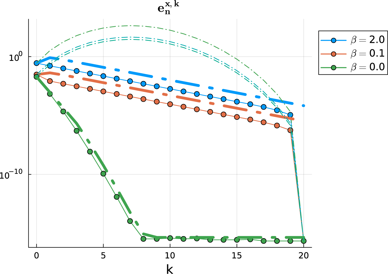
In Figure 1, we display the numerically obtained error
 $e^{x,k} = \max _{1 \leq n \leq N} |x^k_n - x_n|$
, as well as the minimum of the linear and superlinear bounds from Lemma 2.8. We also show the bound based on generating functions in equation (2.10), where we used the infinity norm for
 $\|\cdot \|$
. For this simulation, the decay rate of the fast variable equals
 $\delta = -5$
.
Convergence of micro-macro Parareal for the multiscale ODE test problem, with fine solver the exact solution of equation (2.1) and with coarse solver the forward Euler method applied on equation (2.3) with
 $\bar \alpha = \alpha $
. The decay rate of the fast variable equals
 $\delta = -5$
. Connected circles, numerical simulation; thin dashed line, upper bound from equation (2.10); thick dash-dotted line, minimum of linear and superlinear bounds from equations (2.14) and (2.15). Each colour corresponds to another value of
 $\beta $
.

From Figure 1, we observe that the new bounds from Lemma 2.8 effectively capture the convergence of the slow variable, and that these are more tight than the bound in equation (2.10). If
 $\beta = 0$
, the slow variable is not influenced by the fast variable; in that case, the convergence of the slow variable can be bounded using the classical upper bounds from Gander and Vandewalle [Reference Gander and Vandewalle6] (see Lemma 1.1): then the convergence speed is solely determined by the difference between F and G. As the coupling parameter
 $|\beta |$
increases, the influence of the fast variable (which converges linearly, see Lemma 2.7) on the convergence of the slow variable increases.
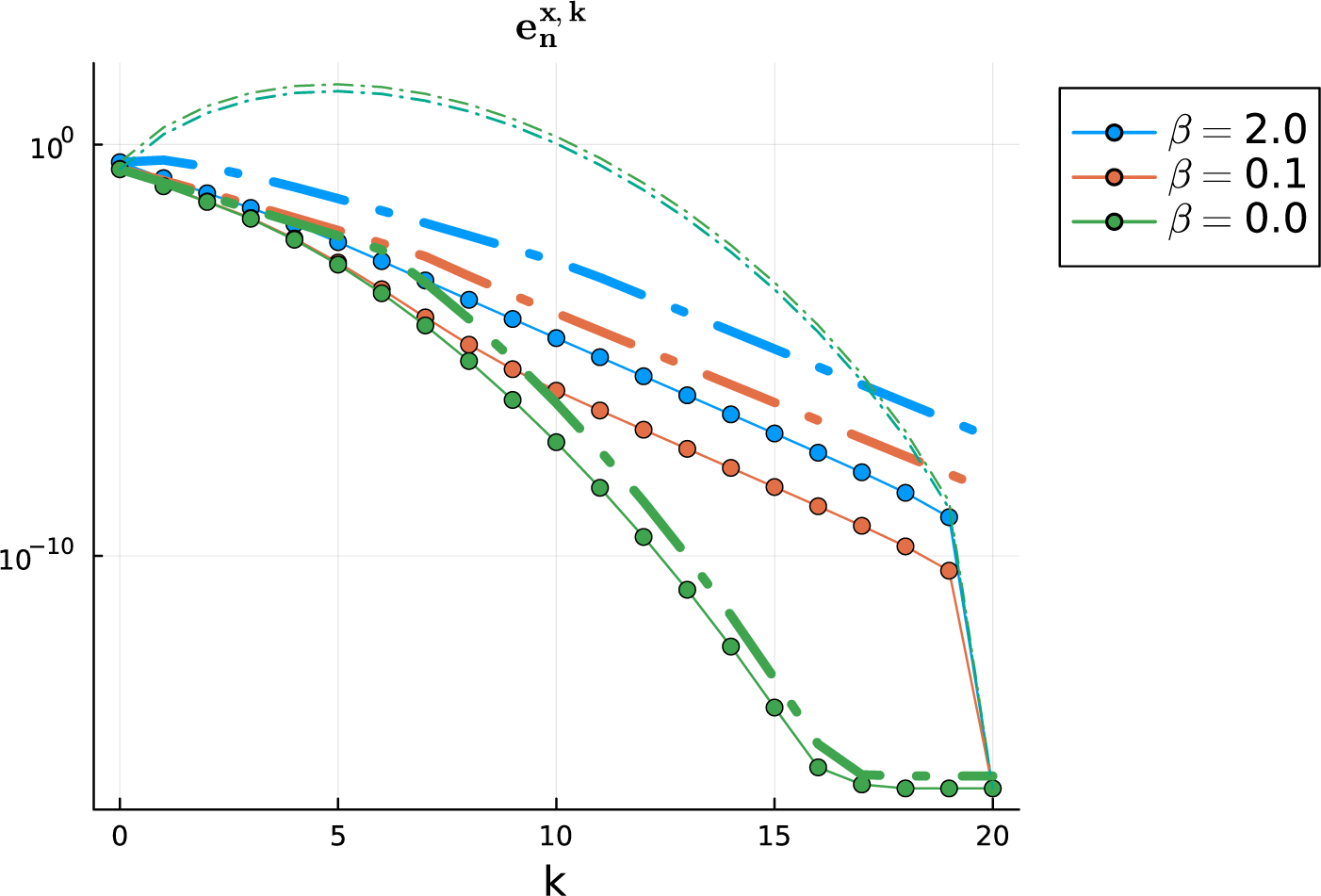
In Figure 2, we study a similar situation, but now, we artificially increase the error in the coarse solver by choosing
 $G = e^{\bar \alpha \Delta t}$
with
 $\bar \alpha = 2 \alpha $
and by putting
 $\delta =-10$
.
Convergence of micro-macro Parareal for the multiscale ODE test problem, with fine solver the exact solution of equation (2.1) and with coarse solver the exact solution to equation (2.3) with
 $\bar \alpha = 2 \alpha $
. The decay rate of the vast variable equals
 $\delta =-10$
. Each colour corresponds to another value of
 $\beta $
.

From Figure 2, we observe the following. If
 $\beta =0$
, the error in the slow variable is solely due to the model error in the coarse solver. As
 $|\beta |$
increases, initially, the error decays much like
 $\beta =0$
, but after the first few iterations, a linear convergence regime sets in. In this linear regime, the error is dominated by the convergence of the fast variable, which Lemma 2.7 has shown to be linear (captured in the second (sum) term of the bounds). As the number of iterations increases, our bounds have the same slope as the numerically obtained slow errors.
Avoiding initial slip. A proper choice of the initial condition
 $\bar x_0$
in equation (2.3) to avoid initial slip, following Van Kampen [Reference Van Kampen14, Appendix A], is
 $$ \begin{align} \bar x_0 = x_0 - y_0 \frac{\beta}{\delta - \alpha}. \end{align} $$
This choice does affect the operators from Definition 2.1. Indeed, if the restriction operator were chosen as
 $\mathcal R ( (x,y) ) = x - y {\beta }/({\delta -\alpha })$
(in line with equation (2.18)) and if the matching operator is the one from Definition 2.1, then it does not hold that
 $\mathcal M ( \mathcal R (u), u) = u$
for any u. This would lead to a violation of the finite termination property (see Property 1).
Alternatively, we can shift the effect of equation (2.18) into the coarse propagator, which then acts on the full micro state variable. If
 $$ \begin{align*} \hat{\mathcal B} = \left[ \begin{matrix} e^{\bar \alpha \Delta t} & -\frac{\beta }{\delta -\alpha}e^{\bar \alpha \Delta t} \\ 0 & 0 \end{matrix} \right], \end{align*} $$
then the following classical Parareal iteration describes the effect of the modified initial condition from equation (2.18):
 $$ \begin{align*} \begin{aligned} u^0_{n+1} &= \hat{\mathcal B} u^0_n , \\ u^{k+1}_{n+1} &= (\mathcal A - \hat{\mathcal B}) u^{k}_{n} + \hat{\mathcal{B}} u^{k+1}_n. \end{aligned} \end{align*} $$
The proof of this equality is similar to the proof of Lemma 2.3. In micro-macro Parareal, this corresponds to the following choices: the micro variable
 $u = ( x, \, y )$
and the macro variable
 $U = (x, \, y)$
, and:
-
• a fine propagator
$\mathcal F: \mathbb R^2 \rightarrow \mathbb R^2: \mathcal F(u) := \mathcal A u$
(see the stiff model in equation (2.1)); -
• a coarse propagator
$\mathcal C: \mathbb R^2 \rightarrow \mathbb R^2: \mathcal C(U) := \hat {\mathcal B} U$
; -
• a restriction operator
$ \mathcal R: \mathbb R^2 \rightarrow \mathbb R^2: \mathcal R (u) := u$
; -
• a matching operator
$ \mathcal M: (\mathbb R^2, \mathbb R^2) \rightarrow \mathbb R^2: \mathcal M((X,Y), (x,y)) := (X,y)$
; -
• a lifting operator
$ \mathcal L: \mathbb R^2 \rightarrow \mathbb R^2: \mathcal L((x,y)) := (x, \, 0) $
.


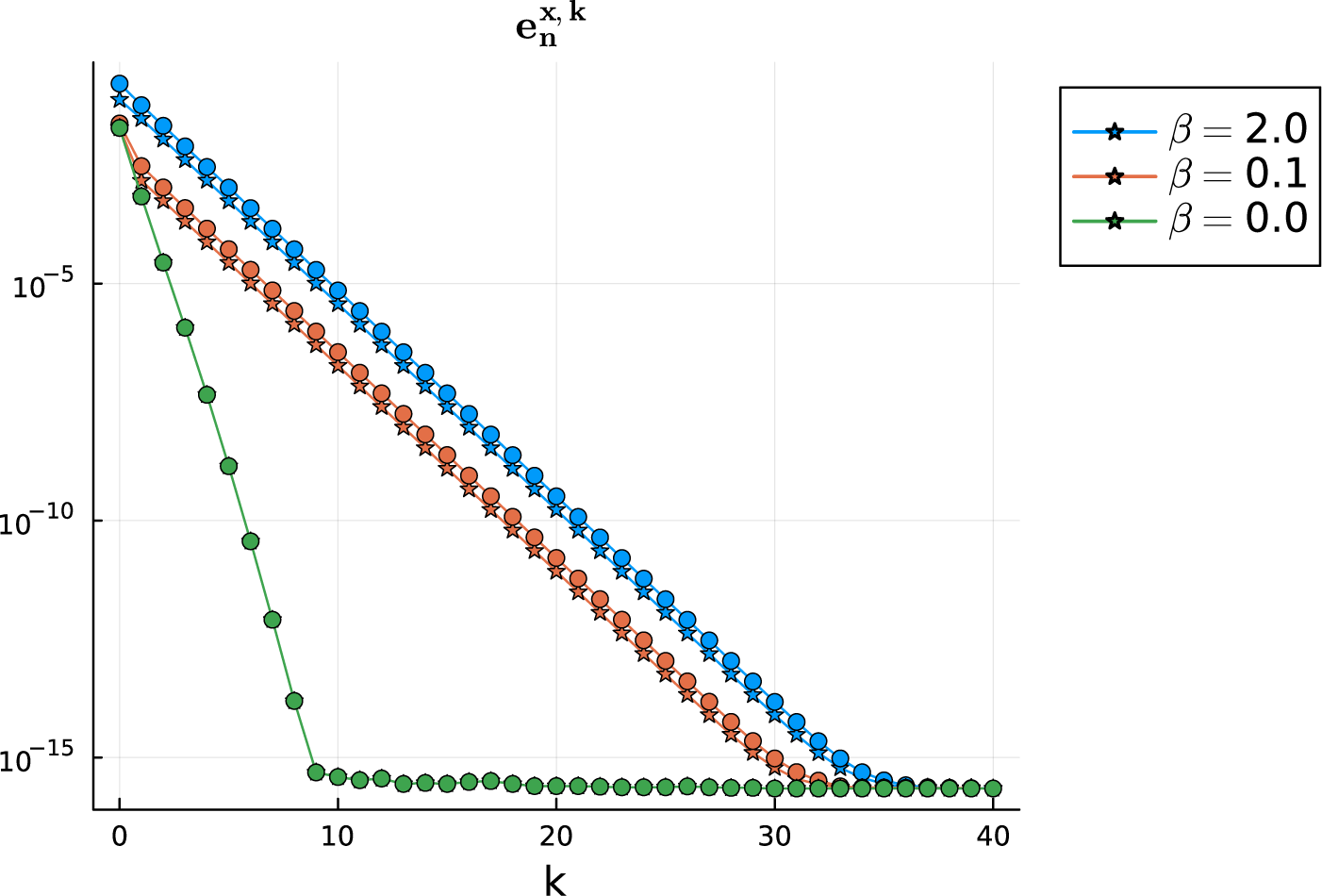
In Figure 3, we can see that this proper choice of initial condition moderately improves the error. A theoretical analysis of this effect, however, is beyond the scope of this work.
Convergence of micro-macro Parareal for the multiscale ODE test problem with
 $\alpha = -1$
and
 $\delta = -10$
. The fine solver is the exact solution of equation (2.1). To study the effect of initial slip on the convergence, the coarse solver is forward Euler on equation (2.3), using
 $\mathcal B$
(filled circles) and using the modified procedure
 $\hat {\mathcal B}$
(star-shaped markers).

3 Monte Carlo-moments Parareal: extension to multidimensional SDEs
In [Reference Bossuyt, Vandewalle and Samaey4], we proposed the Monte Carlo-moments (MC-moments) Parareal method, a micro-macro Parareal algorithm for the simulation of scalar McKean–Vlasov SDEs. In this section, we extend that method to multidimensional SDEs.
3.1 McKean–Vlasov stochastic differential equations
McKean–Vlasov SDEs model the dynamics over time t of an ensemble of P (coupled) particles
 $x^{(p)} \in \mathbb {R}^d$
,
 $p=1 \cdots P$
. The system is defined for some initial distribution of particles
 $p_0$
. Each particle
 $x^{(p)}$
is subject to noise from L independent scalar Wiener processes
 $W^{(l,p)}(t,\omega^{(l,p)})$
, with index
 $1 \leq l \leq L$
, for noise realisations parametrised by
 $\omega^{(l,p)}$
. For notation, these particles are collected in the state variable
 $\bar x = ( x^{(1)}, \ldots , x^{(P)} )$
.
We consider a special class of Mckean–Vlasov SDEs, where the mean-field interaction is the expected value of a function of the particles (for a more general treatment, see, for example, [Reference Sznitman and Hennequin13]). Let
 $\psi $
be some function of the collective state variable, and
 $\Lambda (t) = \mathbb {E}_P[\psi (\bar x(t))]$
, in which
 $\mathbb {E}_P$
is the empirical mean of an ensemble with P particles. For instance, if
 $\psi $
is the identity, then
 $\Lambda $
is just the mean of the particle ensemble. Later, we also use the operator
 $\mathrm {Cov}_P[\bar x]$
, which computes the covariance matrix of the ensemble
 $\bar x$
.
This is the McKean–Vlasov SDE, with P particles,
 $1 \leq p \leq P$
, which we consider:
 $$ \begin{align} \begin{aligned} dx^{(p)} &= a ( x^{(p)}, \Lambda(t), t)\, dt + \sum_{l=1}^L b^{(l)} (x^{(p)}, \Lambda(t), t)\, dW^{(l,p)}, \\ \bar x(0) &\sim p_0, \\ \end{aligned} \end{align} $$
in which the coefficient
 $a: (\mathbb R^d, \mathbb R^d, \mathbb R) \rightarrow \mathbb{R}^d$
is a drift coefficient, and
 $b^{(l)}:(\mathbb R^d, \mathbb R^d, \mathbb R) \rightarrow \mathbb{R}^{d}$
are diffusion coefficients. We use the Itô interpretation of the SDE in equation (3.1).
Assumptions. We only consider SDEs that have a unimodal particle distribution for all
 $t \geq 0$
. For more information about loosening this assumption, see [Reference Bossuyt, Vandewalle and Samaey4].
Simulation. The MC simulation of equation (3.1) is computationally expensive because (i) for accurate results, a lot of particles are required; and (ii) in each time step, the mean of the particles in
 $\Lambda (t)$
needs to be computed.
3.2 Moment ODEs as approximation for multidimensional SDEs
In this section, we aim to obtain a cheap approximation to the McKean–Vlasov SDE in equation (3.1).
We first write a general multivariate Taylor series of the drift and diffusion coefficients for a particle
 $x^{(p)}$
around the mean value
 $\mathbb {E}_P[\bar x]$
:
 $$ \begin{align*} a(x^{(p)}, \Lambda,t) &\approx a(\mathbb{E}_P[\bar x], \Lambda, t) + A_1(\mathbb{E}_P[\bar x], \Lambda,t) (x^{(p)}-\mathbb{E}_P[\bar x])\\ b^{(l)}(x^{(p)}, \Lambda,t) &\approx b^{(l)}(\mathbb{E}_P[\bar x], \Lambda,t) + B_1^{(l)}(\mathbb{E}_P[\bar x], \Lambda,t) (x^{(p)}- \mathbb{E}_P[\bar x]). \end{align*} $$
Here,
 $A_1$
and
 $B_1^{(l)} \in \mathbb{R}^{d \times d}$
are the Jacobian matrices of the drift and diffusion coefficients a and
 $b^{(l)}$
.
This expansion, however, is not practically useful, because it assumes that
 $\Lambda $
is available. A more practical expansion is constructed by approximating
 $\Lambda = \mathbb {E}_P[\psi (\bar x)]$
with
 $\Lambda _{\mathbb {E}_P} = \psi (\mathbb {E}_P[\bar x])$
(the approximation consists in changing the position of the expectation operator).
We now define ODEs for describing the evolution the variables M and
 $\Sigma $
, which aim to closely approximate the mean and the covariance matrix of the particle ensemble. For background theory on these approximations for classical SDEs, see for instance [Reference Rodriguez and Tuckwell12] and [Reference Arnold1]. The variable M approximates the evolution of the mean
 $\mathbb {E}_P[\bar x] \in \mathbb {R}^d$
as
 $$ \begin{align} \begin{aligned} \frac{dM}{dt} &= a(M,\psi(M)) + \frac{1}{2} Q \operatorname{Vec} (\Sigma), \quad M(0) = \mathbb{E}_P[\bar x(0)], \end{aligned} \end{align} $$
where Q is a matrix whose jth row contains a flattened Hessian matrix of the jth component of the drift coefficient a and where
 $\operatorname {Vec}$
is the vectorization (flattening) operator. The evolution of an approximation
 $\Sigma $
to the covariance matrix
 $\mathrm {Cov}[\bar x] \in \mathbb {R}^{d \times d}$
can be described with a matrix differential equation:
 $$ \begin{align} \begin{aligned} \frac{d\Sigma}{dt} &= A_1(M,\psi(M),t)\Sigma + \Sigma A_1(M,\psi(M),t)^T \\[-3pt] & \quad + \sum_{l=1}^L B_1^{(l)} \Sigma B_1^{(l) T} + b^{(l)}(M,\psi(M),t) b^{(l)}(M,\psi(M),t)^{T} \\[-3pt] \Sigma(0) &= \mathrm{Cov}_P[\bar x(0)]. \end{aligned} \end{align} $$
3.3 Coupling operators for multidmensional MC-moments Parareal
Definition 3.1 (MC-moments Parareal for SDEs of any dimension).
The micro variable u is an ensemble of particles
 $u = \bar x$
, and the macro variable U contains its first empirical moments (mean and covariance matrix)
 $U = [\mathbb {E}_P[u], \, \mathrm {Cov}_P[u]]$
. We choose:
-
• a fine propagator
$\mathcal F$
: an MC simulation of the SDE in equation (3.1); -
• a coarse propagator
$\mathcal C$
: (a numerical simulation of) the moment model in equations (3.2)–(3.3); -
• a restriction operator
$\mathcal R( \bar x) := [\mathbb {E}_P[\bar x], \, \mathrm {Cov}_P[\bar x]]$
; -
• a matching operator
$\mathcal M$
that takes as input a particle ensemble
$\bar x$
and a pair of desired mean M and covariance matrix
$\Sigma $
. Let us assume that both
$\mathrm {Cov}_P[\bar x]$
and
$\Sigma $
are positive semidefinite (PSD). Now define the matrices
$V \in \mathbb R^{d \times d}$
and
$Q \in \mathbb R^{d \times d}$
via the Cholesky decompositions
$\Sigma = V V^T$
and
$\mathrm {Cov}_P[\bar x] = Q Q^T$
.-
– If Q is invertible, then we define
$A = V Q^{-1}$
and (3.4)
$$ \begin{align} \mathcal{M}([M, \, \Sigma], \bar x) := A (\bar x - \mathbb{E}_P[\bar x]) + M. \end{align} $$
-
– If Q is not invertible, then the particles
$\bar x$
are resampled from a standard normal distribution;
-
-
• a lifting operator
$\mathcal L$
, used in the zeroth micro-macro Parareal iteration is chosen to be matching with respect to the initial condition of the SDE
$\mathcal {L}(U) := \mathcal {M}(U, \bar x(0) )$
.


If the drift and diffusion coefficients are affine functions in their first two arguments M and
 $\Lambda = \phi (M)$
, and if
 $\phi $
is a linear function as well, then the moment equations (3.2)–(3.3) are an exact description of
 $\mathbb {E}_P[\bar x]$
and
 $\mathrm {Cov}_P[ \bar x]$
. This fact indicates that the choice of
 $\mathcal R$
and
 $\mathcal C$
is sensible.
We now present a lemma that is important in the light of the exactness property of micro-macro Parareal (see Property 1). The proof of this lemma is given in Appendix D.
Lemma 3.2 (Micro-macro consistency of the chosen matching operator).
Let
 $\bar x$
be an ensemble of particles such that
 $\mathrm {Cov}_P[\bar x]$
is symmetric and positive definite. Let
 ${U = \big [ \begin {matrix} M, \Sigma \end {matrix} \big ]}$
be a macro variable, with
 $\Sigma $
PSD. Then, the matching operator in equation (3.4) satisfies
 $\mathcal {R}( \mathcal M( U, u) ) = U$
and
 $\mathcal {M} ( \mathcal R (u), u ) = u$
.
3.4 Numerical experiment
We illustrate the generalized MC-moments Parareal method from Definition 3.1 for a classical SDE without mean-field interaction from the book by Roberts [Reference Roberts11, Exercise 21.6]:
 $$ \begin{align} \begin{aligned} dx &= f(x,y) \,dt, \\ dy &= g(x,y) \,dt + \sigma \,dW , \end{aligned} \quad \left[ \begin{matrix} x(0) \\ y(0) \end{matrix} \right] = \left[ \begin{matrix} 1 \\ 1 \end{matrix} \right], \end{align} $$
with
 $f(x,y) = \alpha x - x y$
and
 $g(x,y) = -y + x^2$
. Our aim is to simulate the SDE over the time interval
 $[0, \, 10]$
. For this choice of initial condition, the solution is unimodal in the whole time domain. Since the noise is additive, the Itô interpretation of equation (3.6) is the same as its Stratonovich interpretation. For the stochastic simulation of the SDE, we use the Euler–Maruyama method (see, for example, [Reference Kloeden and Platen7]) with a time step of
 $\Delta t = 0.02$
on a particle ensemble
 $\bar x$
with
 $10^5$
particles.
For the SDE in equation (3.5), the moment model, defined in equations (3.2)–(3.3), can be written as
 $$ \begin{align} \begin{aligned} \frac{dM_x}{dt} &= f(M_x,M_y) + f_{xy}(M_x, M_y) C_{xy}, \\ \frac{dM_y}{dt} &= g(M_x, M_y) C_{xx} + \frac{1}{2} g_{xx}(M_x, M_y)C_{xx}, \\ \frac{dC_{xx}}{dt} &= 2f_x(M_x,M_y)C_{xx} + 2f_y(M_x,M_y)C_{xy}, \\ \frac{dC_{xy}}{dt} &= f_y(M_x,M_y)C_{yy} + (f_x(M_x,M_y) + g_y(M_x,M_y))C_{xy} + g_x(M_x,M_y)C_{xx}, \\ \frac{dC_{yy}}{dt} &= 2g_y(M_x,M_y)C_{yy} + 2g_x(M_x,M_y)C_{xy} + \sigma^2, \end{aligned} \end{align} $$
with
 $$ \begin{align*} \left[ \begin{matrix} M_x(0) \\ M_y(0) \end{matrix} \right] = \left[ \begin{matrix} 1 \\ 1 \end{matrix} \right], \quad \left[ \begin{matrix} \Sigma_{xx}(0) & \Sigma_{xy}(0) \\ \cdot & \Sigma_{yy}(0) \end{matrix} \right] = \left[ \begin{matrix} 0 & 0 \\ \cdot & 0 \end{matrix} \right] \end{align*} $$
and with
 $f_x = \alpha - y$
,
 $f_y = -x$
,
 $f_{xy}=-1$
,
 $g_x = 2x$
,
 $g_y = -1$
and
 $g_{xx} = 2$
. We choose
 $\alpha = 1$
. The moment ODE is numerically simulated with the forward Euler method with the same time step, using the software by Rackauckas and Nie [Reference Rackauckas and Nie10].
3.4.1 Introductory experiment: quality of the moment model
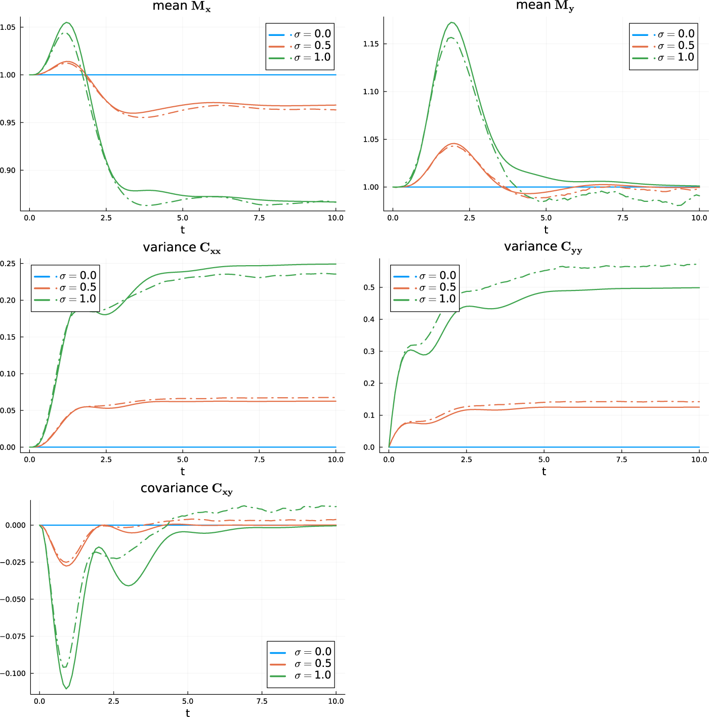
As a way to inspect the quality of the moment ODE, we plot in Figure 4 a numerical solution to the moment ODE together with a numerical solution of the SDE. We observe that the quality of the moment model is not always excellent. The moment model gets more accurate as the noise level
 $\sigma $
goes to zero.


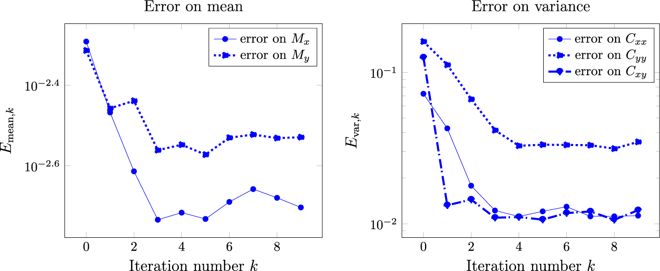
Convergence of modified MC-moments Parareal for the multidimensional SDE in equation (3.5): relative error on mean and variance versus iteration number.

3.4.2 Convergence of MC-moments Parareal
In Figure 5, we plot the relative error on each component of the mean and the variance, measured through an infinity-norm over time, as a function of the iteration number. The errors are computed using an average of 20 realisations, where in each realisation, the fine Parareal solver uses one ensemble
 $\bar x$
of
 $P = 10^5$
coupled particles. We chose the number of Parareal subintervals
 $N = K= 10$
and a time interval
 $[0, 20]$
. The noise level is set to
 $\sigma = 0.5$
.
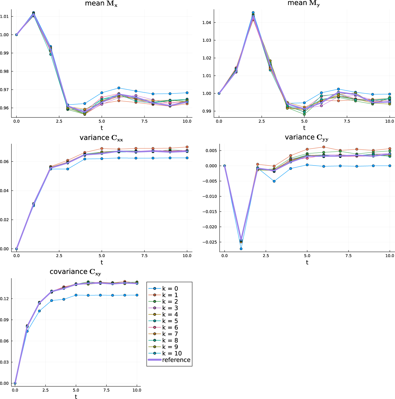
In Figure 6, we plot different Parareal iterates. The final iteration (for which
 $k=N$
), which is indicated with a thick line, serves as the reference solution and corresponds to the sequential simulation in Figure 4. From Figures 5 and 6, we conclude that convergence to the sequential solution takes place. In other experiments, however, we have observed that the speed of convergence is parameter dependent. For instance, changing
 $\sigma $
and/or
 $\alpha $
may lead to nonmonotonic and slower convergence than the convergence observed in Figure 5.
Convergence of modified MC-moments Parareal for the multidimensional SDE in equation (3.5): illustration of the convergence of the moments towards the reference solution. The reference solution is the last iterate of MC-moments Parareal, which corresponds to a sequential simulation with the fine propagator.

4 Conclusion
In Section 2, we presented a new convergence bound for micro-macro Parareal for a special linear multiscale ODE. While our work focuses on a specific case of the multiscale ODEs considered by Legoll et al. [Reference Legoll, Lelièvre and Samaey8], our bound is a generalization of an existing bound for scalar ODEs from Gander and Vandewalle [Reference Gander and Vandewalle6]. It contains an extra term that decreases as the decay rate of the fast component in the ODE system increases. In the future, it would be interesting to develop a convergence bound for a more general class of linear multiscale ODEs, where the bottom left element of
 $\mathcal A$
does not need to be zero. Also, as we considered only
 $x,y \in \mathbb R$
, generalizations to higher dimensions and to more general nonlinear ODEs would be interesting.
In Section 3, we extended a Parareal algorithm in which the fine solver is a Monte Carlo simulation of the SDE, and the coarse solver is an approximate ODE description of the first two statistical moments of the SDE. In the future, it would be interesting to perform tests with the algorithm on more examples, such as true McKean–Vlasov SDEs, and to study the influence of the form of different SDEs on the convergence. Another path would be to augment the MC-moments Parareal method with a way to exploit other reduced models, such as the normal forms described by Roberts [Reference Roberts11].
In summary, we first studied micro-macro Parareal for ODEs, and then we visited a Parareal method for SDEs that exploits ODE descriptions. This journey brought us first to ODEs, and via the SDEs, we returned to ODEs.
Appendix A. Proof of Lemma 2.3
Proof.
-
• First, we observe that for the operators in Definition 2.1, it holds that for any U and u,
$\mathcal R (\mathcal M(U, u)) = U$
and
$\mathcal M ( \mathcal R (u), u) = u$
. Thus, as a result of Property 1, we have
$U^k_n = x^k_n$
for all
$0 \leq n \leq N$
. -
• In the zeroth iteration, it holds that
$$ \begin{align*} \begin{aligned} U^0_{n+1} &= G U^0_n, \\ u^{0}_{n+1} &= \mathcal L (U^0_{n+1}) = \left[ \begin{matrix} G U^0_n \\ 0 \end{matrix} \right] = \left[ \begin{matrix} G x^0_n \\ 0 \end{matrix} \right] = \mathcal B u^{0}_{n}. \end{aligned} \end{align*} $$
-
• In subsequent iterations, it holds that
where
$$ \begin{align*} U^{k+1}_{n+1} &= \mathcal C (U^{k+1}_n) + \mathcal{R} ( \mathcal F (x^k_n)) - \mathcal{C} (U^{k}_n) \\ &= G U^{k+1}_n + F x^k_n + b y^k_n - G U^{k}_n , \\u^{k+1}_{n+1} &= \mathcal M ( U^{k+1}_{n+1}, \mathcal F(x^k_n) ) = \mathcal M \left( U^{k+1}_{n+1}, \left[ \begin{matrix} F x^k_n + by^n \\ d y^k_n \end{matrix} \right] \right) \\ &= \left[ \begin{matrix} U^{k+1}_{n+1} \\ d y^k_n \end{matrix} \right] = \left[ \begin{matrix} G U^{k+1}_n + F x^k_n + b y^k_n - G U^{k}_n \\ d y^k_n \end{matrix} \right] \\ &= \left[ \begin{matrix} G x^{k+1}_n + F x^k_n + b y^k_n - G x^{k}_n \\ d y^k_n \end{matrix} \right] \\ &= (\mathcal A - \mathcal B) u^k_n + \mathcal B u^{k+1}_n, \end{align*} $$
$d = e^{\delta \Delta t}$
.


Appendix B. Solution of a linear recursion
Lemma B.1. Let
 $B, L \in \mathbb {R}^{d \times d}$
be matrices, let
 $\epsilon _0 \in \mathbb {R}^d$
be a vector and
 $b \in \mathbb R$
a scalar, then this iteration for
 $\mathbf e^{x,(k)} \in \mathbb {R}^d$
,
 $$ \begin{align} \mathbf e^{x,(k)} = B \mathbf e^{(k-1)} + b M L^{k-1} \epsilon_0, \end{align} $$
has the solution
 $$ \begin{align} \begin{aligned} \mathbf e^{x,(k)} &= B^{k} \mathbf e^{(0)} + b \sum_{i=0}^{k-1} B^{i} M L^{k-1-i} \epsilon_0. \end{aligned} \end{align} $$
Appendix C. Proof of Lemma 2.6
Commutativity of
 $M^{-1}$
and C. First, we give an expression for
 $M^{-1}$
(the matrix M is defined in equation (2.7)). It is a lower triangular Toeplitz matrix (see [Reference Gander and Vandewalle6]):
 $$ \begin{align*} M^{-1} = \left[ \begin{matrix} I & 0 & 0 & \cdots & & 0\\ \mathcal{B} & I & 0 & \cdots & & 0\\ \mathcal{B}^2 & \mathcal{B} & I & \cdots & & 0 \\ \mathcal{B}^3 & \mathcal B^2 & \beta & \cdots & & 0\\ \vdots & & & & & \vdots \\ \mathcal{B}^{N-1} & \mathcal{B}^{N-2} & \mathcal{B}^{N-3} & \cdots & \mathcal{B} & I \\ \end{matrix} \right]. \end{align*} $$
Let
 $\gamma = \mathcal A - \mathcal B$
, then we have that
 $M^{-1} C$
is a lower-triangular matrix
 $$ \begin{align*} M^{-1} C = \left[ \begin{matrix} 0 & 0 & 0 & \cdots & & 0\\ \gamma & 0 & 0 & \cdots & & 0\\ \mathcal{B} \gamma & \mathcal{B} \gamma & 0 & \cdots & & 0 \\ \mathcal{B}^2 \gamma & \mathcal{B} \gamma & \gamma & \cdots & & 0\\ \vdots & & & & & \vdots \\ \mathcal{B}^{N-2} \gamma & \mathcal{B}^{N-3} \gamma & \mathcal{B}^{N-4}\gamma & \cdots & \gamma & 0 \\ \end{matrix} \right]. \end{align*} $$
However, we have that
 $C M^{-1}$
is a lower-triangular matrix
 $$ \begin{align*} C M^{-1} = \left[ \begin{matrix} 0 & 0 & 0 & \cdots & & 0\\ \gamma & 0 & 0 & \cdots & & 0\\ \gamma \mathcal{B} & \gamma & 0 & \cdots & & 0 \\ \gamma \mathcal{B}^2 & \gamma \mathcal{B} & \gamma & \cdots & & 0\\ \vdots & & & & & \vdots \\ \gamma \mathcal{B}^{N-2} & \gamma \mathcal{B}^{N-3} & \gamma \mathcal{B}^{N-4} & \cdots & \gamma & 0 \\ \end{matrix} \right]. \end{align*} $$
If
 $\gamma $
and
 $\beta $
do commute, then
 $M^{-1}$
and C are commutative.
Proof of other statements. The fact that
 $M^{-1} C = HD$
can be readily checked. Similarly, it can be verified that
 $C M^{-1} = DH$
. Thus, if
 $M^{-1} C = C M^{-1}$
, then
 $HD = DH$
. Thus, if
 $M^{-1}$
and C commute, so do H and D.
Appendix D. Proof of Lemma 3.2
Proof. We first prove that, under the conditions of Lemma 3.2, it is true that
 $\mathcal {R}( \mathcal M( U, u) ) = U$
. Let X be a random variable
 $X \in \mathbb R^d$
with
 $\mathrm {Cov}[X] = Q Q^T$
and Q invertible,
 $M \in \mathbb R^d$
be a vector and
 $\Sigma \in \mathbb R^{d \times d}$
a matrix with
 $\Sigma = V V^T$
. Then, we need to prove that
 $$ \begin{align} \begin{aligned} \mathbb{E}_P[ \mathcal{M}([M, \, \Sigma], X) ] &= M, \\ \mathrm{Cov}_P[ \mathcal{M}([M, \, \Sigma], X) ] &= \Sigma. \end{aligned} \end{align} $$
We name
 $Y = \mathcal {M}([M, \, \Sigma ], X)$
.
-
• Using the linearity of the expectation, we have
(D.2)
$$ \begin{align} \mathbb{E}_P[Y] = \mathbb{E}_P[AX] - A \mathbb{E}_P [X] + M = M. \end{align} $$
-
• Using that for a random variable
$X \in \mathbb R^d$
, with an arbitrary vector
$b \in \mathbb R^d$
and matrix
$A \in \mathbb R^{d \times d}$
,
$\mathrm {Cov}_P[A(X-b)] = A \mathrm {Cov}_P[X]A^T$
, we obtain (D.3)where we used the definition
$$ \begin{align} \mathrm{Cov}_P[Y] &= \mathrm{Cov}_P[A(X-\mathbb{E}_P[X])+M] \notag \\ &= A \mathrm{Cov}_P [X] A^T \notag \\ &= A Q Q^T A^T = VV^T, \end{align} $$
$A = V Q^{-1}$
.


Equations (D.2) and (D.3) prove equation (D.1).
Now, we prove that
 $\mathcal {M} ( \mathcal R (u), u ) = u$
. In this case,
 $A = V Q^{-1} = I$
and
 $M = \mathbb {E}_P[\bar x])$
.
 $$ \begin{align*} \mathcal{M}([\mathbb{E}_P[\bar x], \, \mathrm{Cov}_P[\bar x]], \bar x) = A (\bar x - \mathbb{E}_P[\bar x]) + M = \bar x. \end{align*} $$
This ends the proof.
Acknowledgements
We sincerely thank the anonymous reviewers for their careful and thorough work. Their suggestions have greatly ameliorated this text.
We thank Thibaut Lunet for discussions about convergence of micro-macro Parareal. We thank Thijs Steel for suggesting the Cholesky factorization in the definition of the matching operator in equation (3.4). We also thank Arne Bouillon for his comments on an earlier version of this manuscript.
This project has received funding from the European High-Performance Computing Joint undertaking (JU) under grant agreement No. 955701. The JU receives support from the European Union’s Horizon 2020 research and innovation programme, and from Belgium, France, Germany and Switzerland.