





Highlights
What is already known?
-
• Existing effect size measures like BC-SMD compare SCEDs with group designs but have limitations for count data due to the violation of normality and homoscedasticity assumptions, and sensitivity to the session length or time units when observing target behaviors.
-
• A between-case incidence rate ratio (BC-IRR) has recently been proposed within the generalized linear mixed model (GLMM) framework. However, its computation is relatively complex, and the finite-sample statistical properties of the GLMM-based estimator have not been evaluated.
What is new?
-
• This study introduces a generalized estimating equation (GEE)-based estimator for BC-IRR and systematically compares its performance with the existing GLMM-based estimator.
-
• Large-scale Monte Carlo simulations demonstrate that both the GLMM- and GEE-based estimators provide unbiased estimates of BC-IRR and its standard errors across a wide range of realistic SCED conditions.
Potential impact for RSM readers
-
• The satisfactory statistical properties of BC-IRR enable comparisons of SCED and group design studies, benefiting research syntheses with findings from both designs.
-
• It enhances methodological rigor, providing researchers with two flexible frameworks for estimating effect sizes that are better suited for SCED count data.
1. Between-case incidence rate ratio for single case experimental designs with count outcomes: A Monte Carlo simulation with conditional and marginal models
Single-case experimental designs (SCEDs) assess the treatment effect of an intervention on a small number of cases by repeatedly measuring outcomes over time under multiple conditions manipulated by the experimenter.Reference Kratochwill and Levin 1 These designs involve the manipulation of treatment and control conditions over time and assess causal effects by comparing outcomes observed under treatment conditions to those observed under control conditions. Because SCEDs often rely on direct observation of behavior, count outcomes are very common, such as the number of aggressive behaviors, words read correctly per minute, and digits correct in math practices. Count data are typically non-normal and heteroscedastic because their variance depends on the mean. Consequently, traditional effect sizes that assume normality and homogeneity, such as the standardized mean differences (e.g., Cohen’s d-type effect sizes), are often inappropriate for count data.
In addition, count data typically represent the number of events occurring over a specific period of time, and an incidence rate is computed by dividing the count by the total observation time. Under the assumption that observation time functions as exposure (i.e., the underlying event-generating process is characterized by an incidence rate), the intervention effect should be expressed as a ratio of incidence rates rather than raw counts and therefore should not depend on the duration of the observation session. However, standardized mean differences are highly sensitive to the observation session length.Reference Pustejovsky 2 , Reference Wilson 3 In some cases, researchers fail to report session lengths, further complicating the effect size calculation for count data.
Furthermore, standardized mean differences can confound intervention effect with outcome variances, particularly when variances are not comparable across studies.Reference Baguley 4 – Reference Kim and FerreeJr 7 This issue is especially problematic in meta-analyses of SCEDs because, unlike group designs that often use standardized measures, SCEDs typically rely on direct observation of specific behaviors defined at the level of individual cases, or curriculum-based measures that are tailored to the specific study. An examination of more than 300 SCED studies by Pustejovsky et al. documented substantial heterogeneity in measurement procedures and outcome characteristics across studies, suggesting that outcome variances are unlikely to be directly comparable.Reference Pustejovsky, Swan and English 8 Therefore, standardized mean differences may be less suitable for research synthesis of SCEDs.
To address these issues, researchers have proposed several ratio-based effect sizes for count outcomes in SCEDs, including the log response ratio (LRR),Reference Pustejovsky 9 , Reference Pustejovsky 10 the Bayesian rate ratio (BRR),Reference Batley, Mehta and Hitchcock 11 and the incidence rate ratio (IRR) for count data in SCEDs,Reference Li, Luo, Baek, Thompson and Lam 12 all of which quantify the magnitude of treatment effects as a proportional change between baseline and treatment phases within cases. Unlike the LRR and BRR, the IRR can simultaneously account for baseline trend, trend change, overdispersion, zero-inflation, and measurement dependencies due to autocorrelation and nested data structure at the same time through the flexible framework of generalized linear mixed models (GLMMs).Reference Li, Luo, Baek, Thompson and Lam 12 – Reference Li 14
The development of these ratio-based effect sizes for SCEDs builds on a long history of using proportional effect measures for count outcomes in other disciplines. Outside the SCED literature, ratio-based effect size measures for count outcomes, including the IRR, relative rate ratio, and LRR, have been widely adopted in medicine, epidemiology, and evolutionary biology.Reference Hawken, Potter and Little 15 – Reference Spittal, Pirkis and Gurrin 18 Among these measures, the IRR is the standard effect measure for count outcomes analyzed using Poisson and related generalized linear models (GLMs). In the behavior and social sciences, researchers have increasingly adopted GLMs and GLMMs to analyze count data, highlighting differences in the interpretation of proportional effect sizes like the IRR in GLMs/GLMMs versus additive effect sizes from linear (mixed) models.Reference Coxe, West, Aiken and Little 19 – Reference Grimm and Stegmann 22 Extending this framework to SCEDs, Li et al. found that GLMMs can yield accurate estimates and reliable inferential statistics for treatment effects quantified by the IRR in multiple baseline designs (MBDs) when researchers make sound statistical decisions regarding model selections.Reference Li, Luo and Baek 13
Despite its widespread use as a standard effect size measure for count outcomes and its favorable statistical properties in SCEDs, the IRR developed for SCEDs is inherently a within-case effect size, referred to as the within-case incidence rate ratio (WC-IRR), as it quantifies proportional changes within individual cases. In SCEDs, effect sizes can be conceptualized as either within-case or between-case, depending on how they are computed. Within-case effect sizes contrast conditions (e.g., baseline versus treatment) within a single case, capturing changes over time.Reference Shadish, Hedges, Horner and Odom 23 In contrast, between-case effect sizes compare conditions across multiple cases by incorporating between-case variability, yielding design-comparable effect sizes that are compatible with those used in group designs (e.g., standardized mean differences). Although most SCED effect sizes are within-case measures (e.g., nonoverlap indices and some regression-based indices), a small number of between-case effect sizes have been developed more recently, such as the between-case standardized mean difference (BC-SMD).Reference Hedges, Pustejovsky and Shadish 24 – Reference Swaminathan, Rogers and Horner 27
Following the same structural model used in the development of BC-SMD, Luo et al. proposed the between-case incidence rate ratio (BC-IRR) for AB designs and MBDs.Reference Luo, Li, Baek and Li 28 Unlike WC-IRR, BC-IRR is a marginal, design-comparable effect size that can be synthesized jointly with IRRs from RCTs. A graphical illustration in Appendix is provided for readers who are interested in the conceptual difference between conditional and marginal estimates for IRR. Although Luo et al. established the theoretical foundation of BC-IRR based on GLMMs,Reference Luo, Li, Baek and Li 28 its finite-sample statistical performance has not been evaluated. Furthermore, estimating BC-IRR using GLMMs requires specification of both the fixed-effects and variance–covariance structures because the derived marginal effect depends on both sets of parameters. The increasing complexity of variance–covariance structures may also lead to convergence issues for GLMMs. Given the limited guidance available for specifying random-effects structures in SCEDs, generalized estimating equations (GEEs), which estimate marginal effects directly without specifying between-case random effects structures, provide an alternative and promising modeling framework.Reference Zeger and Liang 29 , Reference Liang and Zeger 30
The purpose of the current study is to systematically evaluate and compare the statistical properties of BC-IRR estimated via the GLMM and GEE and to demonstrate the methods using R with real data. The paper is organized into six main sections. The literature review section briefly introduces the difference between conditional and marginal estimates, and the formal definition of the BC-IRR. The modeling and estimation section outlines the GLMM and GEE frameworks, reviews their performance in small-sample conditions, and discusses small-sample correction methods. The third section presents a simulation study evaluating the performance of both modeling approaches, focusing on the bias of point estimates, bias of standard errors, mean squared error, and coverage rate of BC-IRR. The fourth section demonstrates the application of these models using real data and R code. The final section concludes with a discussion of implications, practical recommendations, study limitations, and directions for future research.
1.1. Causal definition of BC-IRR for SCEDs
The marginal treatment effect aforementioned for SCEDs could be formally defined by utilizing causal inference framework. Let us consider an AB design with m participants and series length of n. For simplicity, assume that all participants enter the treatment phase at time T. This assumption is not required, as the definition also applies to MBDs in which participants enter the treatment phase at different time points. According to Luo et al., BC-IRR is defined as a causal estimand on a ratio scale:

The numerator represents the expected incidence rate at time B if a treatment strategy is implemented between times T and B. The denominator represents the expected incidence rate at time B if the treatment is never adopted. Both the numerator and the denominator are marginal means, representing the average incidence rates across the m participants under the treated and the untreated conditions. Thus, BC-IRR is a marginal effect.
Because the estimand is defined based on potential outcomes, it is necessary to link the potential outcomes to the observed data. The numerator can be directly linked to the observed incidence rate at time B because all participants receive the treatment. However, the denominator, the potential outcome under no treatment at time B, is unobserved and must be estimated using models based on observations from the baseline phase. A key identifiability condition, therefore, is that this potential outcome model is correctly specified. Additional details of the statistical models are presented in Section 2. BC-IRR has been shown to be equivalent to the IRR that would have been obtained in a hypothetical RCT, under the assumption that a never-treated group exists in which the distribution of individual effects, defined as the time-invariant effects unique to each individual, matches that of the treated units in the SCED. Due to space limitations, we do not repeat the detailed derivations here. Readers are referred to Luo et al. for the complete logical and mathematical arguments.Reference Luo, Li, Baek and Li 28
2. Estimation models for BC-IRR
To estimate BC-IRR as defined in Section 1, we consider two methods, one derived from the conditional/subject-specific model of GLMM, the other based on the marginal/population-average model via the GEE approach.
2.1. Generalized linear mixed model
GLMMs are a set of conditional models that integrate the frameworks of GLM and linear mixed models (LMM). Hence, GLMMs could take the source of clustering or nested data structure in SCEDs into account by directly modeling between-case variation using random effects. With an extension to generalized framework, GLMMs could also deal with non-normal outcomes in SCEDs, such as binary, percentage/proportion, count, and rate data using various distributions (e.g., Poisson, negative binomial, binomial, beta-binomial).
We used the following Poisson GLMM to derive BC-IRR from count outcomes in an AB design:

where
${Phase}_{ij}$
 is an indicator variable equal to 0 for control phase and 1 for treatment phase;
${Time}_{ij}$
 is a time variable representing the time (measured either in calendar units or sessions) elapsed from a reference time point. Researchers can choose any time point as a reference time point, which changes the meaning of the intercept
${\beta}_{0j}$
 and its associated variance–covariance components.
${Time}_{ij}^{\prime }$
 is another centered time variable which equals zero at the first observed treatment session, 1 at the second treatment session, and so forth, following the coding proposed by Huitema and McKean.Reference Huitema and Mckean
31
Readers interested in the alternative coding scheme for the treatment-by-time interaction (
${Time}_{ij}^{\prime }$
 ) are referred to Pustejovsky et al.Reference Pustejovsky, Hedges and Shadish
26
Based on this coding scheme,
${e}^{\beta_{0j}}$
 represents the expected outcome level at the reference time point for case j,
${e}^{\beta_{1j}}$
 represents the proportional change per session during the baseline phase,
${e}^{\beta_{2j}}$
 represents the immediate proportional change in the outcome level at the first observed treatment session relative to the projected baseline trend (i.e., the within-case IRR for immediate effect), and
${e}^{\beta_{3j}}$
 represents the trend/slope change after the treatment (i.e., the within-case IRR for trend change). An example coding matrix for all the variables is shown in Table 1, where
$C$
 is the reference time point, the treatment is implemented at time
$T=A$
 , and the outcome
$Y$
 is measured at time point
$B$
 . Based on a multivariate normal assumption for all random coefficients (i.e.,
${\beta}_{0j}-{\beta}_{3j}$
 )

and the coding matrix in Table 1

where
$B-C$
 represents the time elapsed between the reference time point (
$C$
 ) and the outcome measurement occasion
$B$
 , while
$B-A$
 represents the time elapsed between the introduction of treatment and the outcome measurement occasion. To compute BC-IRR, the estimates of the conditional effects (
$\gamma$
 ) and variance/covariance components (
$\sigma$
 ) from the GLMM are substituted into equation (5). The full derivation process for equation (5) can be found in Luo et al.Reference Luo, Li, Baek and Li
28
Example coding matrix for a case with count data

Table 1. Long description
The table consists of six columns and twelve rows of data.
Column headers from left to right are:
1. Measurement occasions (I)
2. Time sub i j
3. Phase sub i j
4. Time prime sub i j Phase sub i j, defined as I minus (C plus 1)
5. B minus A
6. Outcome (Y)
Data rows:
- Occasion 1: Time -5, Phase 0, Time prime 0, B-A is blank, Outcome 1.
- Occasion 2: Time -4, Phase 0, Time prime 0, B-A is blank, Outcome 3.
- Occasion 3: Time -3, Phase 0, Time prime 0, B-A is blank, Outcome 2.
- Occasion 4: Time -2, Phase 0, Time prime 0, B-A is blank, Outcome 4.
- Occasion 5: Time -1, Phase 0, Time prime 0, B-A is blank, Outcome 2.
- Occasion 6 (C): Time 0, Phase 0, Time prime 0, B-A is blank, Outcome 3.
- Occasion 7 (A): Time 1, Phase 1, Time prime 0, B-A 0, Outcome 10.
- Occasion 8: Time 2, Phase 1, Time prime 1, B-A 1, Outcome 9.
- Occasion 9: Time 3, Phase 1, Time prime 2, B-A 2, Outcome 11.
- Occasion 10: Time 4, Phase 1, Time prime 3, B-A 3, Outcome 6.
- Occasion 11: Time 5, Phase 1, Time prime 4, B-A 4, Outcome 9.
- Occasion 12: Time 6, Phase 1, Time prime 5, B-A 5, Outcome 8.
The Poisson GLMM in equation 3 assumes that the conditional mean and variance for the outcome are identical. However, when count data exhibit more variability than predicted by the Poisson model, overdispersion occurs. Failing to account for overdispersion leads to poor model fit and misleading statistical inferences due to underestimated standard errors of regression coefficients.Reference Li, Luo, Baek, Thompson and Lam 12 , Reference Agresti 32 Pustejovsky et al. found that overdispersion is not uncommon for count outcomes in SCEDs.Reference Pustejovsky, Swan and English 8 To accommodate overdispersion, the following Poisson-Gamma mixture model, also called the negative binomial model (NB), has been introduced to analyze overdispersed count data in SCEDs (Li et al., 2025; Li et al., 2024).

With the log link function and the same multivariate assumption for random coefficients
$\beta$
 , the calculation for BC-IRR as shown in equation (5) is exactly the same for the NB model.
2.2. Marginal model via generalized estimating equation
Rather than explicitly modeling the clustering mechanism via random effects as is done with the conditional models of GLMM, marginal models treat within-subject association as a nuisance characteristic of data that should be accounted for to make correct inferences about changes in the population mean response.Reference Liang and Zeger
30
A marginal model for longitudinal data has the following three-part specificationReference Fitzmaurice, Laird and Ware
33
: (1) The marginal expectation
$E\! \left({y}_{ij}|{\boldsymbol{x}}_{ij}\right)={\mu}_{ij}$
 , depends only on the covariates
${\boldsymbol{x}}_{ij}$
 , through a known link function
$g\! \left({\mu}_{ij}\right)={\boldsymbol{x}}_{ij}^{\prime}\boldsymbol{\beta}$
 ; (2) the variance of
${Y}_{ij}$
 , conditional on the covariates, is given by
$Var\! \left({y}_{ij}|{\boldsymbol{x}}_{ij}\right)=\phi v\left({\mu}_{ij}\right)$
 , where
$v\! \left({\mu}_{ij}\right)$
 is a known variance function of the conditional mean
${\mu}_{ij}$
 and
$\phi$
 is a scale parameter; (3) the covariance matrix for the within-subject responses, conditional on the covariates, is given by
${\boldsymbol{V}}_j=\phi {\sqrt{\boldsymbol{A}}}_j\mathrm{Corr}\left({\boldsymbol{Y}}_j\right)\sqrt{{\boldsymbol{A}}_j}$
 , where
${\boldsymbol{A}}_j$
 is a diagonal matrix with components
$v\! \left({\mu}_{ij}\right)$
 , and
$\mathrm{Corr}\! \left({\boldsymbol{Y}}_j\right)$
 is the correlation matrix as the function of a vector of parameters
$\boldsymbol{\alpha}$
 that estimate the correlations of observations within subjects.
When the outcomes in the marginal model are discrete (e.g., binary, count, or ordinal categorical data), there is no convenient specification of the joint distribution of
${\boldsymbol{Y}}_j$
 . Hence, it requires an alternative to maximum likelihood estimation and leads to a method known as GEE. GEE approach essentially views the model as a single-level model and applies statistical corrections to produce standard error estimates that account for clustering.Reference Zeger and Liang
29
,
Reference Liang and Zeger
30
The advantage of GEE is that the covariance structure of the outcome does not have to be correctly specified, meaning that there are far fewer assumptions required compared to random effects models.Reference Zeger, Liang and Albert
34
For the estimation, GEE requires researchers to specify a working correlation matrix
$\mathrm{Corr}\left({\boldsymbol{Y}}_j\right)$
 , a modeling “device” used to describe the association among repeated observations within the same cluster (e.g., measurements within a case in a SCED). The correlation is “working” because it does not need to be correctly specified to get consistent estimates of the marginal parameter estimates. Several working correlation structures are potentially suitable for SCED application, including independence (i.e., no within-case correlation), exchangeable (i.e., constant correlation among all observations within a case), autoregressive (i.e., correlation decays with time lag), and unstructured (i.e., each pair of observations has its own correlation).
After specifying a working correlation structure, an iterative estimation process is started using weighted least squares (quasi-likelihood) by (1) estimating the regression coefficients (
$\boldsymbol{\beta}$
 ) as if data are independent, (2) estimating the parameters (
$\boldsymbol{\alpha}$
 ) in the working correlation matrix to handle clustering, (3) using the estimated working correlation matrix to update the outcome variable covariance matrix (
${\boldsymbol{V}}_j$
 ), (4) using
${\boldsymbol{V}}_j$
 to update estimates of
$\boldsymbol{\beta}$
 ; and (5) continuing this iteration process until convergence and then applying sandwich estimators for standard errors. For an approachable illustration of the full estimation procedure for GEE, readers are referred to McNeish and Stapleton.Reference McNeish and Stapleton
35
In SCEDs, BC-IRR could be estimated by specifying a marginal model using the GEE approach with an appropriate working correlation matrix. The marginal model is specified as follows for count outcomes:

where the Poisson variance function
$v\left({\lambda}_{ij}\right)={\lambda}_{ij}$
 is adopted, and the scale parameter
$\phi$
 could handle potential overdispersion in SCED count outcomes. The working correlation structure
${\boldsymbol{R}}_{\! j}\left(\boldsymbol{\alpha} \right)$
 describes the correlation pattern of observations within-subject with
$\boldsymbol{\alpha}$
 as a vector of association parameters depending on the correlation structure. In our study, we adopt the “independence” correlation structure to avoid convergence issues encountered with very small sample sizes in SCEDs. We note that other correlation structures including, but not limited to, “unstructured”, “autoregressive”, “Toeplitz”, and “exchangeable” are available for the GEE approach. Based on equations (2) and (7),

where
${\beta}_2$
 and
${\beta}_3$
 represent the marginal estimates of the immediate effect and trend change, respectively. A key advantage of the GEE over GLMM is that it does not require specifying the level-2 variance–covariance structure of random effects. The GEE approach could provide robust estimates of standard errors if all relevant predictors are included, regardless of the proper specification of the working correlation matrix of the outcome measurements.Reference McNeish and Harring
36
2.3. Delta methods for standard errors
As BC-IRR is essentially a combination or a transformation of parameter estimates related to the immediate effect and regarding trend change, we need to further calculate its standard error. As outlined in equations ((5)) and (8), the transformation is relatively complex for the GLMM and more intuitive for the GEE approach. To get standard errors for the transformed parameter, the delta method is typically used. The delta method is essentially calculating the variance of the Taylor series approximation of a function (
$G$
 ) of random variables (
$\boldsymbol{x}$
 = (x1, x2, …)) with known variance. The first two terms of the Taylor expansion are an approximation for the function
$G$
 ,

where
${\boldsymbol{\mu}}_x$
 is the mean vector of
$\boldsymbol{x}$
 and
$\frac{d \! \left(G \! \left({\boldsymbol{\mu}}_x\right)\right)}{d \! \left(\boldsymbol{x}\right)}$
 is a vector of partial derivatives of
$G \! \left(\boldsymbol{x}\right)$
 at point
${\boldsymbol{\mu}}_x$
 . We can then approximate the variance of
$G \! \left(\boldsymbol{x}\right)$
 ,

where
$\operatorname{cov} \! \left(\boldsymbol{x}\right)$
 is the known variance–covariance matrix of
$\boldsymbol{x}$
 . The square root of the outcome based on equation 10 is the standard error of the transformed parameter estimate. To calculate the standard errors of BC-IRR estimated by the GEE approach as shown in equation (8),
$G \! \left(\boldsymbol{x}\right)=G \! \left(\boldsymbol{\beta} \right)={e}^{\left({\beta}_2+{\beta}_3\left(B-A\right)\right)}$
 and
$\operatorname{cov} \! \left(\boldsymbol{x}\right)=\operatorname{cov} \! \left(\boldsymbol{\beta} \right)=\operatorname{cov} \! \left({\beta}_2,{\beta}_3\right)$
 . Similarly, to obtain the standard error of BC-IRR estimated by the GLMM as shown in equation ((5)),
$G \! \left(\boldsymbol{x}\right)=G \! \left(\boldsymbol{\gamma}, \boldsymbol{\sigma} \right)$
 and
$\operatorname{cov} \! \left(\boldsymbol{x}\right)=\operatorname{cov} \! \left(\boldsymbol{\gamma}, \boldsymbol{\sigma} \right)$
 . The calculations via the delta method can be conducted using the deltamethod function in the R package msm.Reference Jackson
37
2.4. Performance of GLMM with small sample size
Recent studies have systematically evaluated the performance of GLMMs in the SCED context.Reference Li, Luo, Baek, Thompson and Lam 12 , Reference Li, Luo and Baek 13 , Reference Declercq, Jamshidi and Fernández-Castilla 38 They have demonstrated that GLMMs are promising methods to deal with overdispersed and zero-inflated SCED count data. These studies also provide tailored guidelines for model selection based on the properties of SCED count data. For example, Declercq et al. found that when count data are not overdispersed, Poisson GLMMs can produce accurate estimates of treatment effects evaluated by WC-IRR.Reference Declercq, Jamshidi and Fernández-Castilla 38 In recent simulation studies, Li et al. also found that GLMMs can provide accurate estimates and reliable inferential statistics for treatment effects measured by WC-IRR in MBDs, when researchers select appropriate distributions (e.g., Poisson, negative binomial, zero-inflated Poisson, and zero-inflated negative binomial).Reference Li, Luo and Baek 13 In addition, there are few studies directly comparing the performance of GLMM and GEE under small sample sizes in more general contexts.Reference McNeish and Stapleton 35 , Reference McNeish and Harring 36 They found that GLMM outperforms GEE in terms of standard error bias, coverage rate, and statistical power for both continuous and binary outcomes. More specifically, for both continuous and binary outcomes with a small number of clustering units (≤ 50), GLMM with degrees of freedom adjusted method (i.e., Kenward-Roger adjustment) showed minimal bias in the standard error estimates of fixed effects and had the coverage rate close to the nominal level of 95%.
2.5. Performance of GEE with small sample size
Unlike solid evidence provided for the statistical properties of GLMMs, there have been no direct studies of GEE applied to the SCED context. However, the performance of GEE for correlated binary and continuous data has been well documented. In the large sample framework, it is known that estimates of regression parameters of GEE are generally unbiased regardless of the working correlation matrix, but misspecifications of the working correlation matrix leads to biased estimates of the standard errors of the regression estimates. Thus, it is typical practice to obtain standard errors based on the robust or sandwich estimator proposed by Liang and ZegerReference Liang and Zeger 30 for the variance–covariance matrix of regression coefficients, which is consistent even under misspecification of the working correlation matrix.Reference Zorn 39
With small sample size, previous research found that GEE does not perform well.Reference McNeish and Stapleton 35 , Reference McNeish and Harring 36 , Reference Thompson, Hemming, Forbes, Fielding and Hayes 40 Specifically, McNeish and StapletonReference McNeish and Stapleton 35 found that GEEs had relatively large bias for fixed effects estimates regarding level-2 predictors and cross-level interactions when dealing with a very small number of clustering units (e.g., n = 4). The 95% confidence interval based on the classical GEE with the sandwich estimator for standard errors often produced significant under-coverage across different levels of number of units (n = 4 to 14).
To enhance both parameter estimates and standard errors of the estimates under small sample sizes, several bias correction methods have been proposed.Reference Thompson, Hemming, Forbes, Fielding and Hayes 40 , Reference Paul and Zhang 41 For example, Paul and Zhang demonstrated that by using bias-adjusted approaches, unbiased parameter estimates can be obtained for small to moderate sample sizes (n = 15 to 50).Reference Paul and Zhang 41 Some other researchers have proposed various corrections for the sandwich estimator to obtain accurate statistical inferences for the GEE regression parameter estimators under small sample sizes, including FG (Fay and Graubard),Reference Fay and Graubard 42 GST (Gosho et al),Reference Gosho, Sato and Takeuchi 43 KC (Kauermann and Carroll),Reference Kauermann and Carroll 44 MK (MacKinnon),Reference MacKinnon and White 45 MD (Mancl and DeRouen),Reference Mancl and DeRouen 46 MBN (Morel et al.),Reference Morel and Bokossa 47 PAN (Pan),Reference Pan 48 and WL (Wang and Long).Reference Wang and Long 49 Recently, Thompson et al. compared the performance of several methods to improve the standard error estimates of GEE with binary outcomes in small samples (n = 6 to 54).Reference Thompson, Hemming, Forbes, Fielding and Hayes 40 They found that some bias-corrected standard error methods (i.e., KC and FG standard errors) outperformed others to mitigate this bias when used with an independent working correlation matrix and were robust to the misspecification of the working correlation matrix. However, Thompson et al. noted significant overcorrections for the FG standard error with a very small number of clusters (n = 6),Reference Thompson, Hemming, Forbes, Fielding and Hayes 40 which is also consistent with other findings.Reference Scott, Decamp, Juraska, Fay and Gilbert 50 , Reference Leyrat, Morgan, Leurent and Kahan 51
2.6. Small-sample correction methods
For GLMMs, researchers could use Kenward-RogerReference Kenward and Roger 52 , Reference Kenward and Roger 53 or SatterthwaiteReference Satterthwaite 54 approaches to adjust for standard errors and degrees of freedom of fixed-effects estimates with small sample sizes. Numerous studies have provided illustrations and/or evaluations of these small-sample corrections for multilevel models in psychological and educational research.Reference McNeish and Stapleton 35 , Reference McNeish and Harring 36 , Reference Stroup 55 – Reference Ferron, Bell, Hess, Rendina-Gobioff and Hibbard 57 However, researchers in the social sciences are not familiar with small-sample corrections for the GEE approach, which is an important issue to consider in the calculation of the standard error of BC-IRR.
As mentioned in the review of performance, the sandwich estimator for the standard error in GEE is downwardly biased when the sample size is small. In our study, we chose four corrections that could potentially improve small-sample performance and are able to account for unbalanced designs (e.g., different numbers of measurements across cases) based on previous studies. To understand these corrections, the sandwich estimator of the standard error of
$\boldsymbol{\beta}$
 based on equation (7) is provided:

where
$\boldsymbol{M}$
 is the “meat” of the “sandwich”:
$\boldsymbol{M}=\sum_{j=1}^J{\boldsymbol{D}}_j^{\prime }{\boldsymbol{V}}_j^{-1}{\widehat{\boldsymbol{r}}}_j{\widehat{\boldsymbol{r}}}_j^{\prime }{\boldsymbol{V}}_j^{-1}{\boldsymbol{D}}_j$
 , with
${\boldsymbol{D}}_j={\boldsymbol{X}}_j^{\prime }{\boldsymbol{A}}_j$
 ,
${\boldsymbol{V}}_j=\phi {\boldsymbol{A}}_j^{\frac{1}{2}}{\boldsymbol{R}}_{\! j}\left(\boldsymbol{\alpha} \right){\boldsymbol{A}}_j^{\frac{1}{2}}$
 ,
${\widehat{\boldsymbol{r}}}_j{\widehat{\boldsymbol{r}}}_j^{\prime }=\left({\boldsymbol{Y}}_j-{\widehat{\boldsymbol{\mu}}}_j\right){\left({\boldsymbol{Y}}_j-{\widehat{\boldsymbol{\mu}}}_j\right)}^{\prime }$
 . When sample size is small,
${\widehat{\boldsymbol{r}}}_j{\widehat{\boldsymbol{r}}}_j^{\prime }$
 is downwardly biased and leads to underestimated standard error of
$\boldsymbol{\beta}$
 .
Two classes of corrected sandwich estimators have been proposed to deal with small samples: residual-based correction and design-based corrections.Reference McNeish and Stapleton
35
Residual-based corrections account for the small-sample bias by adding matrixes to the innermost part of
$\boldsymbol{M}$
 in the sandwich estimators, which could inflate the standard errors. For example,
${\boldsymbol{\Phi}}_{KC}$
 is a bias-corrected sandwich estimator proposed by Kauermann and Carroll,Reference Kauermann and Carroll
44
which rewrites the estimator from equation 11 such that

where
${\boldsymbol{H}}_j={\boldsymbol{D}}_j{\left(\sum_{j=1}^J{\boldsymbol{D}}_j^{\prime }{\boldsymbol{V}}_j^{-1}{\boldsymbol{D}}_j\right)}^{-1}{\boldsymbol{D}}_j^{\prime }{\boldsymbol{V}}_j^{-1}$
 .
Other commonly used residual-based corrections include
${\boldsymbol{\Phi}}_{MD}$
 proposed by Mancl and DerouedReference Mancl and DeRouen
46
:

and
${\boldsymbol{\Phi}}_{FG}$
 proposed by Fay and GraubardReference Fay and Graubard
42
:

where
$\boldsymbol{Q}={\boldsymbol{D}}_j^{\prime }{\boldsymbol{V}}_j^{-1}{\boldsymbol{D}}_j{\left(\sum_{j=1}^J{\boldsymbol{D}}_j^{\prime }{\boldsymbol{V}}_j^{-1}{\boldsymbol{D}}_j\right)}^{-1}$
 and
$b$
 is an upper bound for the correction; by default, it has a value of 0.75.
On the other hand, design-based corrections take a different form and include additional additive terms to the sandwich estimator rather than modifying the “meat” of the “sandwich.” The Morel-Bokossa-Neerchal correction (
${\boldsymbol{\Phi}}_{MBN}$
 )Reference Morel and Bokossa
47
is a commonly adopted design-based correction in applied studies, which comprises the sandwich estimator and an additive term:

where
$P$
 is the number of predictors,
$J$
 equals the number of clusters, and
$\phi =\max \left(r, trace\left({\left(\sum_{j=1}^J{\boldsymbol{D}}_j^{\prime }{\boldsymbol{V}}_j^{-1}{\boldsymbol{D}}_j\right)}^{-1}\boldsymbol{M}\right)/P\right)$
 . The default values for
$d$
 and
$r$
 are 2 and 1, respectively. A summary of the sandwich estimator and discussed corrections is provided in Table 2.
Small-sample corrections to the GEE sandwich variance estimator

Table 2. Long description
The table contains four columns: Category, Estimator, Expression, and Key modification.
* Sandwich Category:
- Estimator: L Z (Liang and Zeger).
- Expression: Phi sub L Z = B super minus 1 M B super minus 1.
- Key modification: M = summation from j = 1 to J of D sub j prime V sub j super minus 1 r-hat sub j r-hat sub j prime V sub j super minus 1 D sub j.
* Residual-based Category:
- Estimator: K C (Kauermann and Carroll).
- Expression: Phi sub K C = B super minus 1 M sub K C B super minus 1.
- Key modification: M sub K C = summation from j = 1 to J of D sub j prime V sub j super minus 1 open parenthesis I minus H sub j close parenthesis super minus 1/2 r-hat sub j r-hat sub j prime open parenthesis I minus H sub j prime close parenthesis super minus 1/2 V sub j super minus 1 D sub j.
- Estimator: M D (Mancl and DeRouen).
- Expression: Phi sub M D = B super minus 1 M sub M D B super minus 1.
- Key modification: M sub M D = summation from j = 1 to J of D sub j prime V sub j super minus 1 open parenthesis I minus H sub j close parenthesis super minus 1 r-hat sub j r-hat sub j prime open parenthesis I minus H sub j prime close parenthesis super minus 1 V sub j super minus 1 D sub j.
- Estimator: F G (Fay and Graubard).
- Expression: Phi sub F G = B super minus 1 M sub F G B super minus 1.
- Key modification: M sub F G = summation from j = 1 to J of Diag open brace open parenthesis 1 minus min open brace b, Q sub j j close brace close parenthesis super minus 1/2 close brace D sub j prime V sub j super minus 1 open parenthesis I minus H sub j close parenthesis super minus 1 r-hat sub j r-hat sub j prime open parenthesis I minus H sub j prime close parenthesis super minus 1 V sub j super minus 1 D sub j Diag open brace open parenthesis 1 minus min open brace b, Q sub j j close brace close parenthesis super minus 1/2 close brace.
* Design-based Category:
- Estimator: M B N (Morel et al).
- Expression: Phi sub M B N = Phi sub L Z plus delta phi open parenthesis summation from j = 1 to J of D sub j prime V sub j super minus 1 D sub j close parenthesis super minus 1.
- Key modification: delta = P all over open parenthesis J minus P close parenthesis if J is greater than open parenthesis d plus 1 close parenthesis P; otherwise 1 all over d.
3. Simulation study
3.1. Data generation
Data were simulated using a NB GLMM as shown in equation 6. We varied the following design factors, including series length (
$I$
 ), number of cases (
$J$
 ), immediate effect (
${\gamma}_{20}$
 ), trend change (
${\gamma}_{30}$
 ), variance components (
${\sigma}_{u0}^2$
 ,
${\sigma}_{u1}^2$
 ,
${\sigma}_{u2}^2$
 ,
${\sigma}_{u3}^2$
 ), dispersion (
$\theta$
 ), and the time elapsed between intervention and measurement sessions (
$B-A$
 ). The chosen conditions and associated rationale are similar to the previous simulation studies with SCED count data.Reference Li, Luo and Baek
13
,
Reference Declercq, Jamshidi and Fernández-Castilla
38
Specifically, the number of cases was 4 or 8, and the series length was 10 or 20. This represented a common setting based on reviews of single-case studies.Reference Pustejovsky, Swan and English
8
,
Reference Shadish and Sullivan
58
Following the MBD, the start of the treatment was staggered across cases:
$I$
 = 10 (starting points of the intervention: 3, 4, 6, 7) and
$I$
 = 20 (starting points of the intervention: 6, 8, 12, 14). These intervention starting points were selected to reflect the range of baseline lengths commonly observed in published SCEDs,Reference Shadish and Sullivan
58
including shorter baseline phases that may not fully satisfy current phase-length recommendations according to the What Works Clearinghouse (WWC). The trend in the baseline phase
${\gamma}_{10}$
 = log (1.00), and thus there is no trend in the baseline phase. The immediate effect
${\gamma}_{20}$
 was set to log (1.00), log (2.00), log (6.00), or log (12.00), representing the zero, small, medium, and large treatment conditions, respectively. Although the effect size benchmark has not been established for immediate effect, the chosen conditions from zero to large effects are consistent with the previous simulation study with SCED count outcomes.Reference Li, Luo, Baek, Thompson and Lam
12
,
Reference Declercq, Jamshidi and Fernández-Castilla
38
,
Reference Li and Luo
59
For trend change
${\gamma}_{30}$
 , the zero, medium, and large effects were set to log(1.00), log(1.05), and log(1.10), which leads to the frequency count increasing by 0%, 5%, and 10% for each measurement in the treatment phase, respectively. The values chosen for trend change are based on reanalysis of meta-analyses of SCEDs using GLMMs.Reference Verschuur, Didden, Lang, Sigafoos and Huskens
60
–
Reference Dart, Collins, Klingbeil and McKinley
62
The between-case variance components for the intercept (
${\sigma}_{u0}^2$
 ), baseline trend (
${\sigma}_{u1}^2$
 ), immediate effect (
${\sigma}_{u2}^2$
 ), and trend change (
${\sigma}_{u3}^2$
 ) were paired as [0.1, 0, 0.1,0], [0.3, 0.0003, 0.3, 0.0003], or [0.5, 0.0005, 0.5, 0.0005]. Following the same practice in Moeyaert et al.Reference Moeyaert, Ugille, Ferron, Beretvas and Van den Noortgate
63
the correlations between all random effects were set as −0.5. The 1:1000 ratio of
${\sigma}_{u1}^2$
 and
${\sigma}_{u3}^2$
 versus
${\sigma}_{u0}^2$
 and
${\sigma}_{u2}^2$
 was also determined based on the reanalysis of SCED count data in previous meta-analyses.Reference Verschuur, Didden, Lang, Sigafoos and Huskens
60
–
Reference Dart, Collins, Klingbeil and McKinley
62
Table 3 summarizes all design conditions. The full factorial design resulted in 864 conditions, each with 2,000 independent replications.
Summary of factors and conditions for simulated count data

Table 3. Long description
The table consists of two columns: Parameter and Value.
* Series length (I): 10 (starting points of the intervention: 3, 4, 6, 7) or 20 (starting points of the intervention: 6, 8, 12, 14).
* Number of cases (J): 4 or 8.
* Intercept (gamma sub 00): log 2.
* Baseline trend (gamma sub 10): log 1.00.
* Immediate effect (gamma sub 20): log 1.00, log 2.00, log 6.00, or log 12.00.
* Trend change (gamma sub 30): log 1.00, log 1.05, or log 1.10.
* Between-case variance for intercept (sigma sub u0 super 2), baseline trend (sigma sub u1 super 2), immediate effect (sigma sub u2 super 2), and trend change (sigma sub u3 super 2): [0.1, 0, 0.1, 0], [0.3, 0.0003, 0.3, 0.0003], or [0.5, 0.0005, 0.5, 0.0005].
* Correlations between all random effects: minus 0.5.
* Dispersion parameter (theta): 5 or 10.
* Time elapsed (B minus A): 0, 1, or 5.
To analyze the simulated data, we fitted the NB GLMMs by using the R package glmmTMB
Reference Brooks, Kristensen and van
64
and the GEE models with independent error structures via the R package gee.Reference Carey, Lumley, Moler and Ripley
65
In GEE models, we applied four small-sample corrections in addition to the sandwich estimator, GEE_LZ (
${\boldsymbol{\Phi}}_{LZ}$
 ), to get standard errors of coefficients, including GEE_KC (
${\boldsymbol{\Phi}}_{KC}$
 ), GEE_MD (
${\boldsymbol{\Phi}}_{MD}$
 ), GEE_FG (
${\boldsymbol{\Phi}}_{FG}$
 ), and GEE_MBN (
${\boldsymbol{\Phi}}_{MBN}$
 ). All corrections were implemented using the R package geesmv.Reference Wang
66
For GLMMs, we allowed all variance components and only one covariance between random intercept and immediate effect to be freely estimated to avoid convergence issues. Hence, the fitted GLMMs were under-specified regarding the level-2 variance–covariance structure, which allows us to examine the robustness of GLMMs to misspecification. For both GLMM and GEE, each model was estimated using two reference time points (C), namely, the first and last sessions of the baseline phase, whereas the data were consistently generated with C at the last session of the baseline phase. This allows us to examine whether BC-IRR is robust to different coding strategies adopted for
${Time}_{ij}$
 . Standard errors of BC-IRRs for both models were computed via the delta method using the R package msm.Reference Jackson
37
The simulation code is available at https://osf.io/eqa4h/?view_only=98358eeef01f4d20b043d902e8d16c0a.
3.2. Performance measure
For each simulated condition, estimator performance was evaluated with four metrics. Bias of the BC-IRR was computed as the mean difference between the estimated and true BC-IRR across the 2,000 replications, as well as the mean-squared error (MSE), which is the sum of the estimator’s variance and squared bias. We calculated the bias of the model-based standard error (SE) from the GEE approach as the difference between the mean reported SE and the empirical standard deviation of BC-IRR estimates. Finally, we evaluated the 95% confidence-interval coverage for the small-sample corrections found effective in Section 2, defined as the proportion of replications whose Wald interval for BC-IRR contains the true value. Sampling variability in coverage was calculated with exact binomial error bounds:
$.95\pm 1.96\sqrt{\frac{0.95\left(1-0.95\right)}{2000}}=\left(.94,.96\right)$
 , so deviations outside this range showed under- or over-coverage beyond Monte Carlo error. To quantify simulation uncertainty, we calculated Monte Carlo standard errors (MCSEs) for each performance measure following the framework outlined by Morris et al.Reference Morris, White and Crowther
67
3.3. Results
To facilitate comparison of the two estimation models, we summarized the differences between the GLMM and GEE across the simulation conditions. Overall, both methods produced negligible bias. Across all design conditions, the median bias was −0.0005 for the GLMM and 0.0004 for the GEE, whereas the mean bias was 0.001 for both methods. Bias ranged from −0.093 to 0.167 for the GLMM and from −0.137 to 0.137 for the GEE. Furthermore, 83.6% of the GLMM conditions and 92.2% of the GEE conditions produced absolute bias smaller than 0.05, indicating that differences in point estimate bias between the two approaches were negligible. The smallest differences in bias occurred when the time elapsed between treatment introduction and outcome measurement was short (particularly when
$B-A=0$
 ) and the between-case intercept variance was small (
${\sigma}_{u0}^2=0.10$
 ). Larger differences emerged as the follow-up duration increased and the between-case intercept variance became moderate or large (
${\sigma}_{u0}^2=0.30$
 or
$0.50$
 ). Even under these conditions, however, the practical differences between the two estimators remained modest, with bias generally ranging from approximately −0.03 to 0.04 across the most influential design factors.
For estimation accuracy, the GLMM was consistently more efficient than the GEE. The median MSEs were 0.19 for the GLMM and 0.26 for the GEE, with corresponding interquartile ranges of 0.21 and 0.27, respectively. Differences in MSE were smallest under the conditions with longer series (
$I=20$
 ), larger numbers of cases (
$J=8$
 ), and shorter follow-up durations after treatment introduction. In contrast, the largest differences occurred under the conditions when the series length was short (
$I=10$
 ), the number of cases was small (
$J=4$
 ), and the follow-up duration was longest (
$B-A=5$
 ). Under these conditions, both estimators exhibited increased MSE, although the GEE consistently showed lower efficiency than the GLMM.
In Figure 1, we compare the bias of the SE of the BC-IRR using six different methods. The GLMM, along with the KC and MD corrections for sandwich estimators in GEE, yielded the lowest bias. The SE bias ranged from −0.728 to 0.013 for the GLMM (Median = −0.035, Mean = −0.047, The interquartile range (IQR) = 0.03, MCSE = 0.008), from −0.444 to 0.412 for the KC correction (Median = −0.048, Mean = −0.035, IQR = 0.07, MCSE = 0.01), and from −0.044 to 0.467 for the MD correction (Median = 0.021, Mean = 0.045, IQR = 0.07, MCSE = 0.011). In contrast, the GEE_FG correction showed the most extreme bias, ranging from −0.054 to 12.100 (Median = 0.50, Mean = 0.86, MCSE = 0.023), with the largest variability across conditions (IQR = 0.87), reflecting systematic over-correction of the SE. The GEE_LZ (Median = −0.130, Mean = −0.161, MCSE = 0.01) and GEE_MBN (Median = 0.058, Mean = 0.079, MCSE = 0.01) methods showed moderate bias but were not stable across conditions, exhibiting wide ranges and IQRs (0.13 and 0.15, respectively).
Boxplot of the standard error bias of BC-IRR.

Figure 1. Long description
The Y-axis is labeled Bias of the standard error with numerical increments from -0.5 to 1.0. The X-axis is labeled S E methods and lists six categories. From left to right, the data shows.
* G L M M. A very narrow box centered slightly below 0.0 with a long tail of outliers extending down to -0.5.
* G E E underscore L Z. A box positioned between -0.1 and -0.2 with a dense cluster of outliers extending below -0.5.
* G E E underscore F G. The largest box in the set, spanning from approximately 0.2 to 1.0 with a median line at 0.5.
* G E E underscore K C. A box centered just below 0.0 with symmetrical outlier whiskers extending both up to 0.4 and down to -0.4.
* G E E underscore M D. A small box positioned just above 0.0 with a vertical line of outliers reaching up to 0.5.
* G E E underscore M B N. A box centered near 0.1 with significant outlier distributions extending both up toward 0.9 and down toward -0.5.
As GLMM, GEE_KC, and GEE_MD yielded more accurate estimates and higher stability across all conditions for SEs than other estimators, we only calculated the coverage rate of BC-IRR for the three estimators as shown in Figure 2. The median coverage rates for BC-IRR under the GLMM and the MD-corrected SEs are nearly identical (.92 versus .91; MCSE = 0.006 and 0.005, respectively), with tight IQRs of .03 and .02, respectively. In comparison, the KC adjustment yields a slightly lower median coverage rate (.87; MCSE = 0.006) and wider IQR (.06).
Boxplot of the coverage rate of BC-IRR.

Figure 2. Long description
The y-axis is labeled Coverage rate with values from 0.8 to 1.0. The x-axis is labeled S E methods with three categories.
* G L M M: The box is positioned between 0.9 and 0.94 with a median around 0.92. It has a long lower whisker extending to 0.85 and several outliers reaching down to 0.83.
* G E E underscore M D: The box is narrower and positioned similarly to G L M M with a median around 0.91. It has a shorter lower whisker and a few outliers between 0.85 and 0.88.
* G E E underscore K C: This box is much larger, spanning from 0.85 to 0.90 with a median around 0.87. It has a very long upper whisker reaching near 1.0 and a dense cluster of outliers extending down to 0.73.
Next, to evaluate the impact of design factors on performance measures, we conducted mixed two-way ANOVA in which the between-condition factors were series length
$I$
 , number of cases
$J$
 , immediate-effect magnitude
${\gamma}_{20}$
 , trend change magnitude
${\gamma}_{30}$
 , between-case variance of the intercept
${\sigma}_{00}^2$
 , and dispersion
$\theta$
 , while the within-condition factor included the estimation strategy (only in ANOVAs with bias and MSE), standard error estimators (only in ANOVAs with SE bias and coverage rate), time elapsed (
$B-A$
 ) and reference time point (
$C$
 ). Main effects and all two-way interactions were tested, with
${\eta}^2$
 statistics reported. All effects that were reported in the Results section had statistical significance at the α = .05 level. To concentrate on the most consequential sources of variation, we used scree-type plots of the ordered
${\eta}^2$
 values to find main effects and interaction terms that fall to the left of the “elbow” point, which is analogous to using the scree plots to determine the number of factors in exploratory factor analyses (Li, 2024).
The bias of BC-IRR was mainly impacted by the time elapsed (
$F\left(2,554\right)=2518.41$
 ,
${\eta}^2=.19$
 ) and the interaction of the intercept variance and the time elapsed (
$F\left(4,554\right)=1344.96$
 ,
${\eta}^2=.20$
 ). As depicted in Figure 3, when the between-case variance of the intercept was set at its smallest level (
${\sigma}_{00}^2=0.1)$
 , the bias remained at the lowest level across different conditions of time elapsed. For the medium and large intercept-variance levels (
${\sigma}_{00}^2=0.3\;\mathrm{or}\;0.5$
 ), the mean bias increases as time elapsed increases. Although the main and interaction effects were statistically significant, there were no meaningful differences, with the bias ranging from −0.03 to 0.04, indicating that the BC-IRR was practically unbiased throughout the design space.
Bias of BC-IRR as a function of time elapsed and variance of the intercept.

Figure 3. Long description
The figure consists of three vertical panels arranged from left to right. All panels share a common y-axis labeled Mean bias ranging from -0.02 to 0.04 and a common x-axis labeled Time elapsed (B minus A) with discrete points at 0, 1, and 5.
Panel 1 (Left): Titled Variance of Intercept (sigma sub u 0 squared) = 0.1. The data shows a slight downward trend. At time 0, mean bias is approximately 0.005. It decreases slightly at time 1 and drops to approximately -0.005 at time 5.
Panel 2 (Center): Titled Variance of Intercept (sigma sub u 0 squared) = 0.3. The data shows an upward trend. At time 0, mean bias is approximately -0.012. It rises to approximately -0.005 at time 1 and increases sharply to approximately 0.025 at time 5.
Panel 3 (Right): Titled Variance of Intercept (sigma sub u 0 squared) = 0.5. The data shows a steep upward trend. At time 0, mean bias is at its lowest point of approximately -0.028. It rises to approximately -0.012 at time 1 and increases very sharply to its peak of approximately 0.042 at time 5.
The MSE of BC-IRR was mainly impacted by time elapsed (
$F\left(2,554\right)=3059.73$
 ,
${\eta}^2=.24$
 ), series length (
$F\left(1,237\right)=4458.61$
 ,
${\eta}^2=.18$
 ), and the number of cases (
$F\left(1,237\right)=3567.22$
 ,
${\eta}^2=.14$
 ). As shown in Figure 4, MSE increases when the time elapsed increases from zero to five. Regarding series length, MSE tends to decrease as the series length increased from 10 to 20. Similarly, increasing the number of cases consistently lowers the MSE across all design conditions.
MSE of BC-IRR as a function of time elapsed, number of cases, and series length.

Figure 4. Long description
The grid is organized into two columns and three rows. The y-axis for all panels is Mean squared error with increments of 0.3, 0.6, and 0.9. The x-axis for all panels is Number of cases (J) with values 4 and 8.
Column 1: Series length (I) = 10.
* Top panel (Time-elapsed (B minus A) = 0): A line starts at approximately 0.35 for 4 cases and decreases to 0.2 for 8 cases.
* Middle panel (Time-elapsed (B minus A) = 1): A line starts at approximately 0.4 for 4 cases and decreases to 0.2 for 8 cases.
* Bottom panel (Time-elapsed (B minus A) = 5): A steep line starts at approximately 1.1 for 4 cases and decreases to 0.5 for 8 cases.
Column 2: Series length (I) = 20.
* Top panel (Time-elapsed (B minus A) = 0): A line starts at approximately 0.25 for 4 cases and decreases to 0.15 for 8 cases.
* Middle panel (Time-elapsed (B minus A) = 1): A line starts at approximately 0.25 for 4 cases and decreases to 0.15 for 8 cases.
* Bottom panel (Time-elapsed (B minus A) = 5): A line starts at approximately 0.35 for 4 cases and decreases to 0.2 for 8 cases.
Overall, M S E decreases as the number of cases increases, and the error is significantly higher when the series length is shorter and the time-elapsed interval is larger.
As shown in Figure 5, the bias of the standard error for BC-IRR was impacted mostly by standard error methods (
$F\left(5,1385\right)=1127.53$
 ,
${\eta}^2=.30$
 ) and its interaction with immediate effect (
$F\left(15,1385\right)=171.78$
 ,
${\eta}^2=.14$
 ). The GEE_FG correction exhibited the largest positive bias, which deteriorated exponentially as the immediate effect increased from 0 to 2.48. GEE_MBN correction showed overestimation, while GEE_LZ showed underestimation across different settings. The GLMM estimator, as well as the KC and MD corrections for GEE’s SE, showed minimal bias and were relatively insensitive to the magnitude of the immediate effect.
Bias of SE as a function of SE methods and immediate effect.

Figure 5. Long description
The figure consists of six panels arranged in a two-by-three grid. The y-axis for all panels is Bias of the standard error, ranging from 0.0 to 1.5. The x-axis is Immediate effect gamma sub 2 0, with discrete values at 0, 0.69, 1.79, and 2.48.
Top row from left to right:
* G L M M: Shows a flat horizontal line near 0.0 across all x-axis values.
* G E E underscore L Z: Shows a flat horizontal line slightly below 0.0.
* G E E underscore F G: Shows a sharp exponential increase, starting near 0.2 at x equals 0 and rising to approximately 1.8 at x equals 2.48.
Bottom row from left to right:
* G E E underscore K C: Shows a mostly flat line near 0.0 with a slight upward tick at the final data point 2.48.
* G E E underscore M D: Shows a flat horizontal line near 0.0.
* G E E underscore M B N: Shows a very slight linear increase, starting near 0.0 and ending just above 0.1 at x equals 2.48.
From the preceding analysis of SE bias, we only include the standard errors based on GLMM, as well as KC and MD corrections for GEE, all of which showed minimal bias, for calculating the coverage rate. The SE methods (
$F\left(2,554\right)=6905.16$
 ,
${\eta}^2=.34$
 ) and the number of cases (
$F\left(1,237\right)=3750.37$
 ,
${\eta}^2=.19$
 ) were largely associated with coverage rate. In Figure 6, with four cases, the GLMM’s SE and MD-based intervals had coverage rates close to the nominal .95 band (mean = .91 and .90, respectively), whereas KC-based interval showed under-coverage (mean = .85). Increasing the number of cases to eight improved coverage rates for each method, with GLMM to .93, MD to .92, and KC to .90. Overall, all methods showed under-coverage across conditions.
Coverage rate of BC-IRR as a function of se methods and number of cases.

Figure 6. Long description
A multi-panel figure with three vertical panels. The y-axis is shared across all panels, labeled Coverage rate, with percentage increments from 86% to 92%. The x-axis for each panel is labeled Number of cases (J) with two discrete points: 4 and 8.
* The first panel, G L M M, shows a linear increase from approximately 91% at J equals 4 to nearly 93% at J equals 8.
* The second panel, G E E underscore K C, shows the steepest linear increase, starting at approximately 84.5% at J equals 4 and rising to just below 90% at J equals 8.
* The third panel, G E E underscore M D, shows a linear increase from approximately 90% at J equals 4 to approximately 92% at J equals 8.
All three methods demonstrate a positive correlation between the number of cases and the coverage rate.
4. An empirical example
In this section, we demonstrated the estimation of BC-IRR using data from a single-case study reported by Ota and DuPaul.Reference Ota and DuPaul 68 We first described the empirical data set, then outlined the model specification and step-by-step procedure for computing BC-IRR together with its standard errors and confidence intervals and finally interpreted the resulting effect sizes. The annotated R script used for the analysis is available at https://osf.io/eqa4h/?view_only=98358eeef01f4d20b043d902e8d16c0a.
4.1. Data
Ota and DuPaulReference Ota and DuPaul 68 evaluated a computer-assisted mathematics program with a game format for three fourth- to sixth-grade students who have attention-deficit hyperactivity disorder (ADHD). An MBD across participants was used: each student completed a series of baseline typical mathematics instruction sessions followed by an intervention phase in which students used 20-minute computer sessions three to four times per week. For every session, the investigators recorded two curriculum-based measures, including Digits Correct per Minute (DCPM) and Problems Correct per Minute (NPCPM), For illustrative purposes, we used the DCPM outcome only, and raw data of the three participants were extracted from the graphs presented in the original paper, as shown in Figure 7.
Performance in DCPM for three students with ADHD during baseline and a computer-assisted intervention, adapted from Ota and DePaul. Reference Ota and DuPaul 68 .

Figure 7. Long description
The graph consists of three vertically stacked panels. The y-axis for all panels is labeled Digits Correct Per Minute D C P M with increments of 10 from 20 to 40. The x-axis is labeled Session with increments from 1 to 16. Vertical dashed lines indicate the transition from baseline to intervention.
* Top panel Matthew. Baseline sessions 1 to 5 show scores fluctuating between 15 and 23. Intervention begins at session 6. Scores immediately jump to 33 and remain relatively stable between 26 and 33 until session 15, where the score rises to 38.
* Middle panel David. Baseline sessions 1 to 9 show a variable trend between 20 and 31. Intervention begins at session 10. Scores start at 36, dip slightly to 32 at session 12, then peak at 45 at session 14 before dropping to 32 at session 15.
* Bottom panel Andrew. Baseline sessions 1 to 12 show a stable but low trend fluctuating between 18 and 24. Intervention begins at session 13. Scores show a modest increase, peaking at 26 at session 15 and ending at 23 at session 16.
4.2. Considerations for effect size selection
For the choice of design-comparable effect size in research synthesis, the BC-SMD is not ideal for this study. Within the primary study, math performance was assessed using two different session lengths (DCPM based on 2-minute sessions and NPCPM based on 5-minute sessions). Prior work has shown that SMDs are sensitive to observation session length, and scaling the scores to a per-minute metric does not fix the problem, where the standard deviation remains a function of session length (Pustejovsky, 2019). As a result, SMDs may not be strictly comparable even across outcomes within the same study.
Beyond the primary study, in a subsequent meta-analysis in which this study was included (DuPaul et al., 2012), outcomes across SCED studies encompassed a wide range of measurement types, including curriculum-based measures, direct observations, percentage of work completed, and counts of words written. Because these measures differ substantially in scale and variance, BC-SMD is not directly comparable across studies and may misrepresent relative intervention impacts. This measurement heterogeneity motivates the adoption of the alternative effect size, BC-IRR, which is less sensitive to between-outcome and between-study differences in outcome variability and observation procedures.
4.3. Model specification
The equations (5) and 8 define BC-IRR within fully specified GLMM and GEE models that account for the baseline trend, immediate effect, and trend change. However, analysts often fit parsimonious models in practice. A reduced specification may reflect substantive knowledge about real data patterns or be imposed by non-convergence issues for complicated models. For demonstration purposes, we illustrated the computation of BC-IRR using GLMM and GEE under three realistic scenarios with increasing complexities. For GEE models, we used two different SE methods, including GEE_KC and GEE_MD, which showed more favorable statistical properties in the simulation study. In Scenario 1, we assume that there is no baseline trend or trend change, while the immediate effect varies across individuals. The GLMM is specified as follows (Model 1):

Based on this GLMM, the formula for BC-IRR is

The GEE is specified as follows, with
${\boldsymbol{R}}_{\! j}\left(\boldsymbol{\alpha} \right)$
 being the independence working correlation structure (Model 2):

Based on the specified GEE, the formula for BC-IRR is

In Scenario 2, we assume that there is a fixed baseline trend, a fixed trend change, and varying immediate effects. The GLMM model is specified as follows (Model 3):
${Y}_{ij}\sim Poisson\;\left({\lambda}_{ij},\theta \right)\; or\;{Y}_{ij}\sim Negative\kern0.17em Binomial\;\left({\lambda}_{ij},\theta \right)$

$\mathrm{Level}\;1:\log \left({\lambda}_{ij}\right)={\beta}_{0j}+{\beta}_{1j}{Time}_{ij}+{\beta}_{2j}{Phase}_{ij}+{\beta}_{3j}{Time}_{ij}^{\prime }{Phase}_{ij}$


Based on this GLMM, the formula for BC-IRR is simplified to

The GEE is specified as follows, with
${\boldsymbol{R}}_{\boldsymbol{j}}\left(\boldsymbol{\alpha} \right)$
 being the independence working correlation structure (Model 4):

Based on the specified GEE, the formula for BC-IRR is

In Scenario 3, we assume that there are varying baseline trends, immediate effects, and trend changes, and only the covariance between the random intercept and the random immediate effect is modeled. The model is specified as follows (Model 5):
${Y}_{ij}\sim Poisson\;\left({\lambda}_{ij},\theta \right)\;\mathrm{or} \ {Y}_{ij}\sim Negative\kern0.17em Binomial\;\left({\lambda}_{ij},\theta \right)$

$\mathrm{Level}\;1:\log \left({\lambda}_{ij}\right)={\beta}_{0j}+{\beta}_{1j}{Time}_{ij}+{\beta}_{2j}{Phase}_{ij}+{\beta}_{3j}{Time}_{ij}^{\prime }{Phase}_{ij}$


Based on this model, the formula for BC-IRR is simplified to

The GEE (Model 6) for Scenario 3 is the same as Scenario 2 (see equation 22) and the resulting BC-IRR formula is the same as well (see equation 23).
The coding of the variables used in these models is the same as that shown in Table 1. For the second and third scenarios where
$B-A$
 (i.e., time elapsed between the introduction of treatment and the outcome measurement occasion) should be identified for BC-IRR calculation, multiple durations were applied including
$B-A=3$
 (shortest treatment duration of this study) and
$B-A=9$
 (longest treatment duration of this study). Models were fitted and analyzed using glmmTMB package version 1.1.11,Reference Brooks, Kristensen and van
64
gee package version 4.13.29,Reference Carey, Lumley, Moler and Ripley
65
geesmv version 1.3,Reference Wang
66
and saws version 0.9.7.0Reference Fay and Graubard
42
in R version 4.5.0. Standard errors of BC-IRRs were computed based on the delta method, using the msm package in R .Reference Jackson
37
4.4. Convergence and test of overdispersion
To determine whether a NB model should be used in GLMM-based BC-IRR calculation, overdispersion was tested after fitting the Poisson model in each scenario for the GLMM. Then the Pearson’s Chi-squared test was conducted to test overdispersion. For Scenarios 1 and 2, the test results indicated that there was no significant overdispersion in the count outcome based on the Poisson model (Model 1:
${\chi}^2=19.98, df=41,p=.99$
 , Model 3:
${\chi}^2=19.71, df=39,p=.99)$
 . Thus, Poisson models were selected for Scenarios 1 and 2. For Scenario 3, the Poisson GLMM (Model 6) failed to converge due to a non-positive-definite Hessian matrix when estimating fixed-effect SEs. All GEE models with Poisson mean specification converged successfully across the three scenarios.
4.5. Results
Table 4 summarizes the parameter estimates from both the conditional GLMMs and the marginal GEEs, together with their corresponding BC-IRRs. For brevity, we do not interpret coefficients of the GLMM and GEE models. Our focus is on the calculation and interpretation of the final BC-IRR values. Detailed explanations of the GLMM parameters can be found in Li et al. (2025). The GEE coefficients are interpreted and used to obtain BC-IRR.
Parameter estimates and BC-IRR for models 1 to 6

Table 4. Long description
The table is organized into five columns: Model, Parameter, Estimate, S E, and 95% C I.
Scenario 1 includes:
* Model 1-G L M M: gamma sub 00 (3.11), gamma sub 10 (0.30), sigma squared sub u0 (0.006), sigma squared sub u1 (0.004), sigma sub u1 u2 (0.005), and B C - I R R (1.36).
* Model 2-G E E (K C-adjusted): beta sub 0 (3.11), beta sub 1 (0.33), and B C - I R R (1.39).
* Model 2-G E E (M D-adjusted): beta sub 0 (3.11), beta sub 1 (0.33), and B C - I R R (1.39).
Scenario 2 includes:
* Model 3-G L M M: gamma sub 00 (3.12), gamma sub 10 (0.002), gamma sub 20 (0.27), gamma sub 30 (0.008), sigma squared sub u0 (0.006), sigma squared sub u2 (0.003), sigma sub u0 u2 (0.005), B C - I R R (B minus A equals 3) (1.34), and B C - I R R (B minus A equals 9) (1.41).
* Model 4-G E E (K C-adjusted): beta sub 0 (3.14), beta sub 1 (0.007), beta sub 2 (0.27), beta sub 3 (0.002), B C - I R R (B minus A equals 3) (1.31), and B C - I R R (B minus A equals 9) (1.32).
* Model 4-G E E (M D-adjusted): beta sub 0 (3.14), beta sub 1 (0.007), beta sub 2 (0.27), beta sub 3 (0.002), B C - I R R (B minus A equals 3) (1.31), and B C - I R R (B minus A equals 9) (1.32).
Scenario 3 includes:
* Model 5-G L M M: Listed as Non-convergence.
* Model 6-G E E: Listed as having the same results as Model 4.
4.5.1 GLMM results
For Scenario 1, based on equation 17, the parameters used to calculate BC-IRR are the immediate effect (
${\gamma}_{10}=.30)$
 , the variance of the random effects associated with immediate effect (
${\sigma}_{u1}^2=0.004)$
 , and the covariance between the baseline intercept and immediate effect (
${\sigma}_{u0u1}=0.005)$
 . The estimated BC-IRR was exp (0.30 + 0.004/2 + 0.005) = 1.36, indicating that the expected (marginal) rate ratio between the baseline and the treatment phase across all cases is 1.36 on average. This means that the DPCM (Digits correct per minute) on average increased by (1.36–1)*100% = 36% after the treatment across all cases (SE = 0.10, 95% CI = 1.18–1.57). In this scenario, BC-IRR remains constant across all durations of the treatments because there is no trend in the treatment phase.
For Scenario 2, based on equation 21, the parameters used to calculate BC-IRR are the immediate effect (
${\gamma}_{20}=0.27)$
 , trend change (
${\gamma}_{30}=.008)$
 , the variance of the random effect associated with immediate effect (
${\sigma}_{u2}^2=0.003)$
 , and the covariance between the baseline intercept and shift in level treatment effect (
${\sigma}_{u0u2}=0.005)$
 . For example, when B-A = 3, the estimated BC-IRR was exp [0.27 + (0.008 * 3) + 0.003/2 + .005] = 1.34, indicating the DPCM increased by 34% on average across all cases after 4 sessions of intervention (SE = 0.18, 95% CI = 1.04–1.73). This effect is comparable to the effect that would have been obtained from a potential RCT in which participants in the treatment group are consecutively treated for 4 sessions and the outcomes measured immediately after session 4 are compared with those from a never-treated control group.
For Scenario 3, the GLMM did not converge due to a non-positive-definite Hessian matrix when estimating SEs of fixed effects.
4.5.2. GEE results
For Scenario 1, based on equation 19, the parameter used to calculate BC-IRR is the marginal shift in level treatment effect (
${\beta}_1=0.33$
 ). The estimated BC-IRR was exp (0.33) = 1.39, indicating the DPCM increased by 39% on average after the treatment across participants (KC-adjusted SE = 0.02, 95% CI = 1.34–1.44; MD-adjusted SE = 0.02, 95% CI = 1.35–1.43).
For Scenarios 2 and 3 using the GEE model, based on equation 23, the parameter used to calculate BC-IRR is the marginal immediate effect (
${\beta}_2=0.27$
 ) and the marginal trend change (
${\beta}_3=0.002)$
 . For example, when B-A = 3, The estimated BC-IRR was exp (0.27 + 0.002*3) = 1.31, indicating that the DPCM increased 31% on average across all cases after 5 sessions (KC-adjusted SE = 0.09, 95% CI = 1.13–1.51; MD-adjusted SE = 0.10, 95% CI = 1.14–1.51). Similarly, with GLMM-based BC-IRR, this effect is comparable to the effect that would have been obtained from a potential RCT in which participants in the treatment group are consecutively treated for 4 sessions and the outcomes measured immediately after session 4 are compared with those from a never-treated control group.
5. Discussion
The present study systematically evaluated the statistical properties of BC-IRR when estimated via GLMMs and GEEs. Through a Monte Carlo simulation, we assessed the bias, MSE, and coverage rate of BC-IRR estimators and compared the performance of various estimators for their SEs with GLMM and GEE. We also included a real-data demonstration by calculating BC-IRR, its SEs, and confidence intervals under different model specifications based on researchers’ prior knowledge under commonly encountered scenarios.
Overall, the simulation results suggest that both GLMM and GEE approaches yield accurate estimates of BC-IRR across various conditions. Although BC-IRR tends to be slightly overestimated when the time elapsed
$B-A$
 increases and the intercept variance becomes relatively large, the magnitudes of the bias are still trivial and meaningless in practice. Similarly, the SEs of BC-IRR based on GLMM, and two corrections with GEE_KC and GEE_MD are relatively unbiased, whereas biased standard error estimates are found with the sandwich estimator GEE_LZ, and the other two corrections with GEE_FG and GEE_MBN. Notably, the GEE_FG shows significant overcorrections for standard errors in small samples, which aligns with previous findings.Reference Thompson, Hemming, Forbes, Fielding and Hayes
40
,
Reference Scott, Decamp, Juraska, Fay and Gilbert
50
,
Reference Leyrat, Morgan, Leurent and Kahan
51
Both point estimates and standard error estimates of BC-IRR are not sensitive to the different choices of the reference point C and the misspecification of the level-2 variance–covariance structure (only for GLMM). The robustness of BC-IRR against potential misspecification allows researchers to adjust model specifications to resolve convergence issues without sacrificing estimation accuracy. Regarding the efficiency of BC-IRR estimators, GLMMs are slightly more efficient than GEE, while significantly lower efficiency is observed for both when the series length is 10 and the
$B-A$
 is 5.
For interval estimates, BC-IRR shows substantial under-coverage relative to the nominal level of 95% across all examined methods. When the number of cases is 8, the coverage rates are close to the nominal level for GLMM and GEE_MD. This finding is consistent with the known limitations of Wald-type confidence intervals in small samples. The Wald confidence intervals are adopted due to the lack of well-defined degrees of freedom for BC-IRR under either GLMM or GEE. We also caution that the interval estimate of BC-IRR should not be used for the purpose of statistical inferences of treatment effectiveness for a single study, not only because of the under-coverage found in the simulation, but also the inconsistency between the design in the null hypothesis (i.e., a hypothetical group-based design) and the data obtained from a single-case study. For statistical inferences in a single study, researchers should adopt WC-IRR, to evaluate the effectiveness of treatments on a typical case (i.e., all random effects = 0) or cases with the same random effects.
Based on the theoretical framework, simulation results, and observed convergence issues, we provide the following recommendations for researchers to calculate BC-IRR and obtain standard errors in their own study: (1) when researchers use GLMM to calculate BC-IRR and its standard error, determine the complexity of level-2 covariance structures based on prior theory and/or visual analyses. Starting from Scenario 2 or 3 is recommended to mitigate convergence problems; (2) if convergence issues are encountered or level-2 variance–covariance structures are difficult to specify, consider using GEE with an independent working correlation structure. For more accurate standard error estimates, GEE_KC or GEE_MD are recommended; and (3) When calculating BC-IRR, researchers should first determine the follow-up duration of substantive interest because the effect size is defined at a specific time elapsed after treatment (
$B-A$
 ). When treatment effects are expected to evolve over time, reporting BC-IRRs for multiple observed values of
$B-A$
 is recommended. The selected
$B-A$
 values should not exceed the longest treatment duration observed across cases, because doing so requires extrapolating the treatment trend beyond the observed data. In addition, the reference time point (
$C$
 ) can be chosen for convenient coding (e.g., the first or last baseline session), as our simulation indicates that BC-IRR is robust to the choice of
$C$
 .
Overall, the BC-IRR shows strong promise for synthesizing findings from SCEDs and those from group-based designs. The present study, together with previous studies.Reference Li, Luo, Baek, Thompson and Lam 12 – Reference Li 14 , Reference Luo, Li, Baek and Li 28 , Reference Declercq, Jamshidi and Fernández-Castilla 38 further highlights the potential of the GLMM framework for modeling SCED count data, while also extending to a marginal modeling approach through the use of GEEs. Collectively, these studies provide solid evidence supporting the favorable statistical properties of ratio-type effect sizes in SCEDs, including unbiased point estimates and adequate control of Type I error rates, with WC-IRR and BC-IRR serving complementary but distinct research purposes.
With respect to the selection of design-comparable effect size measures, BC-IRR may serve as a viable alternative to BC-SMD, particularly in the presence of substantial non-normality, under which biased estimates may arise.Reference Chen, Pustejovsky, Klingbeil and Van Norman 69 In addition, the BC-SMD index is known to be highly sensitive to the choice of divisor unit.Reference Pustejovsky 2 , Reference Wilson 3 Therefore, when studies to be synthesized rely on heterogeneous time units (e.g., session lengths ranging from seconds to minutes) to observe target behaviors, BC-IRR may outperform BC-SMD because time units cancel out naturally for ratio-type effect sizes.
5.1. Limitations and future directions
Given that the calculation for BC-IRR relies on multiple fixed effects and variance components in the GLMM and that the undesirable statistical properties found for the GEE approach with small sample sizes in previous studies, the results from our study under the SCED context are very encouraging for further methodological studies. The findings are constrained by the selected simulation conditions, which, although typical in MBDs, may not generalize to other research contexts or designs. In addition, benchmarks for the magnitude of immediate effects and trend changes used in the simulation have not yet been fully established. Ongoing work by our team aims to develop domain-specific benchmarks to better inform realistic simulation conditions for both WC-IRR and BC-IRR in SCEDs. Stronger connections between these benchmarks and visual analysis conventions remain to be established. Advancing this line of work will require contributions from SCED researchers with expertise in both statistical modeling and visual analysis.
Another limitation of the present study is that the onset of intervention was pre-specified rather than determined through a response-guided design. Previous methodological studies suggest that response-guided intervention rules primarily influence the characteristics of the baseline data, particularly baseline variability, and do not necessarily introduce substantial bias into multilevel-model treatment effect estimates.Reference Joo, Ferron, Beretvas, Moeyaert and Van den Noortgate 70 , Reference Swan, Pustejovsky and Beretvas 71 An additional note is that the population BC-IRR expression does not depend directly on the between-case variance of the baseline intercept or baseline trend. Thus, baseline heterogeneity alone is not expected to directly influence the population estimand of BC-IRR. Nevertheless, response-guided intervention rules may affect the finite-sample estimation of these model parameters, and the performance of BC-IRR estimators under various response-guided algorithms remains unknown. Future research should evaluate the robustness of the proposed estimators under such designs. To release the full potential of calculating BC-IRR with an aim to synthesize results from both SCEDs and group-based designs, there are several important issues yet to be investigated. A thorough investigation of these issues is beyond the scope of this study, but we discuss them here to suggest directions for future research.
5.2. Bayesian approach
In practice, researchers applying BC-IRR in SCEDs using GLMMs may face convergence challenges or difficulty specifying variance–covariance structures. While GEEs offer a marginal modeling approach that can address some of these concerns, experienced researchers may still prefer GLMMs when prior theory or visual inspection supports their use, especially for improved efficiency. Bayesian estimation presents a promising alternative in this context. R packages such as brms Reference Bürkner 72 and GLMMadaptive Reference Rizopoulos 73 allow Bayesian GLMM fitting and offer tools to derive marginal estimates from conditional ones. Future studies should investigate the convergence properties and small-sample bias of BC-IRR estimates under a Bayesian framework.
5.3. Degrees of freedom of BC-IRR
Although standard error estimates of BC-IRR via GLMM, GEE_KC, and GEE_MD are relatively unbiased, their associated Wald confidence intervals have exhibited poor coverage. A critical unresolved issue is how to appropriately define degrees of freedom for BC-IRR, given its reliance on multiple components from GLMM or GEE. The Satterthwaite approximationReference Satterthwaite 54 may offer a viable solution, given its favorable statistical properties found in dealing with small samples in SCED contexts (citations). Deriving Satterthwaite-type degrees of freedom for composite effect sizes like BC-IRR could be considered for future methodological work.
5.4. Outcome scales
This study focused on count outcomes, which are frequently observed in SCEDs. However, other outcome types, such as rates, proportions, percentages, and ordinal or continuous scores from surveys, are also common. These varied outcome scales complicate synthesis across studies, as different distributions (e.g., Gaussian, Poisson, Binomial) entail different assumptions about the relationship between the mean and variance. Multilevel modeling frameworks have been adapted to produce appropriate effect sizes for these outcome types, yet the incompatibility of obtained effect sizes can hinder meta-analyses aiming to aggregate diverse findings. The GEE-based BC-IRR, which makes no distributional assumptions, may provide a solution. Future research should explore the performance of GEE-based proportional effect sizes when applied to counts, rates, proportions/percentages, and continuous outcomes.
Author contributions
Conceptualization: H.L., C.L., W.L., E.B.; Formal analysis: C.L., H.L.; Funding acquisition: W.L., H.L., E.B.; Methodology: H.L.; Project administration: W.L.; Software: H.L., C.L.; Supervision: H.L.; Visualization: H.L., C.L.; Writing—original draft: H.L., C.L., W.L., E.B.; Writing—review and editing: H.L., C.L., W.L., E.B.
Competing interests
The authors declare that the research was conducted in the absence of any commercial or financial relationships that could be construed as a potential competing interests.
Data availability statement
The data used for the demonstration and the R codes are available at https://osf.io/eqa4h/?view_only=98358eeef01f4d20b043d902e8d16c0a.
Funding statement
The research reported here is supported by the Institute of Education Sciences, U.S. Department of Education, through Grant (R305D240019) to Texas A&M University. The opinions expressed are those of the authors and do not represent views of the Institute or the U.S. Department of Education.
A. Appendix
A.1. Conditional and marginal estimates for IRR
The different interpretations between the WC-IRR and BC-IRR in the analysis of SCED count data originate from the statistical decision on whether it is more appropriate to use a conditional model or a marginal model to analyze correlated response data. An extensive and ongoing discussion exists in disciplines such as statistics, biology, ecology, and epidemiology regarding the differences, advantages, and limitations of these two modeling approaches. However, the conceptual and technical nuances of both models may remain opaque to researchers in the behavioral and social sciences.
To facilitate understanding, we begin with a general illustration of conditional and marginal estimates, followed by an example specific to SCEDs. We first consider a two-level linear mixed-effects model (LMM), which can be written as:
${y}_{ij}={\boldsymbol{x}}_{ij}^{\prime}\boldsymbol{\beta} +{\boldsymbol{z}}_{ij}^{\prime }{\boldsymbol{u}}_j+{e}_{ij}$
 ,
${\boldsymbol{u}}_j\sim N\left(0,\boldsymbol{G}\right)$
 , and
${e}_{ij}\sim N\left(0,{\sigma}_e^2\right)$
 , where
${y}_{ij}$
 denotes a continuous outcome for unit
$i$
 in cluster
$j$
 ,
${\boldsymbol{x}}_{ij}$
 denotes a vector of covariates and
$\boldsymbol{\beta}$
 is the associated vector of regression coefficients,
${\boldsymbol{z}}_{ij}$
 denotes a vector including an intercept and a subset of the unit-level covariates in
${\boldsymbol{x}}_{ij}$
 and
${\boldsymbol{u}}_j$
 is the associated vector of cluster random effects, assumed multivariate normally distributed with zero mean vector and variance–covariance matrix
$\boldsymbol{G}$
 , and
${e}_{ij}$
 is the residual, assumed normally distributed with zero mean and residual variance
${\sigma}_e^2$
 . A distinctive feature of the LMM is that it has simple expressions for both the conditional mean response for an individual given by
$E\! \left({y}_{ij}|{\boldsymbol{x}}_{ij},{\boldsymbol{z}}_{ij},{\boldsymbol{u}}_j\right)={\boldsymbol{x}}_{ij}^{\prime}\boldsymbol{\beta} +{\boldsymbol{z}}_{ij}^{\prime }{\boldsymbol{u}}_j$
 , and the marginal mean response averaged over random effects
${\boldsymbol{u}}_j$
 given by
$E\! \left({y}_{ij}|{\boldsymbol{x}}_{ij},{\boldsymbol{z}}_{ij}\right)={\boldsymbol{x}}_{ij}^{\prime}\boldsymbol{\beta}$
 . The same component
${\boldsymbol{x}}_{ij}^{\prime}\boldsymbol{\beta}$
 means that in LMMs, the fixed effects
$\boldsymbol{\beta}$
 have both subject-specific and population-average interpretations. For example, if
${\boldsymbol{x}}_{ij}^{\prime }$
 contains only a binary treatment indicator (0 = control, 1 = treatment), then
$\boldsymbol{\beta}$
 represents both (a) the conditional difference in outcomes between individuals with the same random effects (e.g., typical individual with
${\boldsymbol{u}}_j$
 = 0) and (b) the average treatment effect across the population. However, having both conditional and marginal interpretations is generally not the case for
$\boldsymbol{\beta}$
 when a non-linear function is adopted in the GLMM framework.
Consider the corresponding GLMM with a non-normal outcome
${y}_{ij}$
 :
${y}_{ij}\!\! \mid \!\! {\boldsymbol{x}}_{ij},{\boldsymbol{z}}_{ij},{\boldsymbol{u}}_j\!\! \sim \!\! \mathrm{Distr}\;\left({\lambda}_{ij},\mathrm{A}\left({\lambda}_{ij}\right)\right),G \! \left({\lambda}_{ij}\right)={\boldsymbol{x}}_{ij}^{\prime}\boldsymbol{\beta} +{\boldsymbol{z}}_{ij}^{\prime }{\boldsymbol{u}}_j$
 , where
${\lambda}_{ij}$
 represents the expected value of the outcome
${y}_{ij}$
 conditional on the predictors
${\boldsymbol{x}}_{ij}^{\prime }$
 and random effects
${\boldsymbol{u}}_j$
 ,
$\mathrm{A}\! \left({\lambda}_{ij}\right)$
 is the variance function and its form depends on the theoretical distribution (
$\mathrm{Distr}$
 ), and
$G \! \left(\bullet \right)$
 is a non-linear link function (e.g., log or logit link function). In this model, the conditional mean response is
$E\! \left({y}_{ij}|{\boldsymbol{x}}_{ij},{\boldsymbol{z}}_{ij},{\boldsymbol{u}}_j\right)={g}^{-1} \! ({\boldsymbol{x}}_{ij}^{\prime}\boldsymbol{\beta} +{\boldsymbol{z}}_{ij}^{\prime }{\boldsymbol{u}}_j)$
 , while the marginal mean response, averaged over
${\boldsymbol{u}}_j$
 , is
$E\! \left({y}_{ij}|{\boldsymbol{x}}_{ij},{\boldsymbol{z}}_{ij}\right)\ne {g}^{-1} \! \left({\boldsymbol{x}}_{ij}^{\prime}\boldsymbol{\beta} \right)$
 and often lacks a closed-form solution. Thus, the fixed effects
$\boldsymbol{\beta}$
 in GLMMs only have a conditional interpretation, but do not have a marginal interpretation as in the LMM. However, for count data modeled with Poisson or negative binomial distributions, approximate or numerical methods can be used to derive marginal estimates based on GLMMs.
In SCEDs, consider the following Poisson GLMM for count outcomes:

where i and j are the indices of repeated measures and cases, respectively, and Phase is a binary variable (0 = baseline and 1 = treatment). The intercept
${\gamma}_{00}$
 represents the within-case baseline level and
${\gamma}_{10}$
 represents the within-case treatment effect in the log-count scale because the log link function is adopted. The effect size for the treatment effect in the frequency count scale is assessed by exp (
${\gamma}_{10}$
 ), which is a within-case effect size (i.e., WC-IRR). The between-case variance components (
${\sigma}_{u0}^2$
 and
${\sigma}_{u1}^2$
 ) are found on the diagonal of the variance–covariance matrix (i.e., the G matrix), representing the variance of the baseline level and the treatment effect between cases. The off-diagonal element (
${\sigma}_{u0u1}$
 ) represents the covariance between baseline level and the treatment effect. To facilitate the understanding of the differences between conditional and marginal estimates, we first provide the expressions for the conditional and marginal expectations based on the Poisson GLMM in Table A1 (see Leckie et al., 2020).
Expressions for the conditional and marginal expectations of the count outcome in a two-level random coefficients GLMM

Table A1. Long description
The table consists of a header row and one data row labeled Expression.
1. The first column header is blank. The corresponding data cell is labeled Expression.
2. The second column header is Conditional expectation. The expression is: exp open parenthesis bold x sub i j prime bold beta plus bold z sub i j prime bold u sub j close parenthesis.
3. The third column header is Marginal expectation. The expression is: exp open parenthesis bold x sub i j prime bold beta plus bold z sub i j prime bold G bold z sub i j close parenthesis.
For simplicity, the following illustration focuses on the conditional and marginal estimates for the treatment effect (
${\gamma}_{10}$
 ). Assuming
${\gamma}_{10}=1.77$
 and
${\sigma}_{u1}^2=0.30$
 . Hence, the conditional treatment effect for a typical case (i.e., a median case with
${\boldsymbol{u}}_j=\boldsymbol{0}$
 ) measured by WC-IRR is
$\frac{\exp \left({\gamma}_{00}+{\gamma}_{10}\right)}{\exp \left({\gamma}_{00}\right)}=\exp \left({\gamma}_{10}\right)=\exp (1.77)=5.86$
 , meaning that the expected outcome level is multiplied by a factor of 5.96 for a typical case after the intervention. On the other hand, the marginal treatment effect for the population is
$\frac{\exp \left({\gamma}_{00}+{\gamma}_{10}+{\sigma}_{u0}^2/2+{\sigma}_{u1}^2/2\right)}{\exp \left({\gamma}_{00}+{\sigma}_{u0}^2/2\right)}=\exp \left({\gamma}_{10}+{\sigma}_{u1}^2/2\right)=\exp \left(1.77+\frac{0.30}{2}\right)=6.82$
 , meaning that, on average across cases, the expected outcome level after the intervention is multiplied by a factor of 6.82, which is comparable to IRRs reported in group-based designs. A graphic illustration of the transformation between the log scale and the original data scale in terms of treatment effect estimates is depicted in Figure A1. It is noted that the marginal effect estimated from the GLMM is subject to accuracy for both fixed and random effects estimates. An alternative way to estimate the marginal effect like BC-IRR for SCED count outcomes is through direct marginal modeling.
Graphical illustration of conditional and marginal estimates.

Figure A1. Long description
Two side-by-side density plots illustrate the transformation of statistical estimates.
Left Panel: Titled Distribution of Log Case Means. The x-axis ranges from 0 to 4 and the y-axis represents Density. A symmetric, bell-shaped curve is centered at x equals 1.77. A solid vertical line passes through the peak, which is labeled with the normal distribution notation N(gamma sub 10 = 1.77, sigma sub u 1 super 2 = 0.30).
Right Panel: Titled Distribution of Case Means on the Data Scale. The x-axis ranges from 0 to 30 and the y-axis represents Density. The curve is highly right-skewed with a long tail extending toward the higher values. Two vertical lines mark specific estimates. A solid vertical line at x equals 5.86 is labeled median case: exp(gamma sub 10) = 5.86. To its right, a dotted vertical line at x equals 6.82 is labeled marginal mean: exp(gamma sub 10 + sigma sub u 1 super 2 / 2) = 6.82. The marginal mean is positioned further into the right tail than the median case.
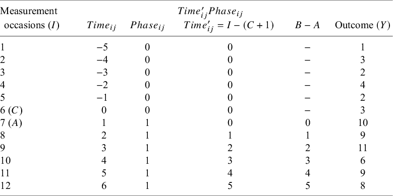
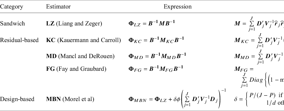
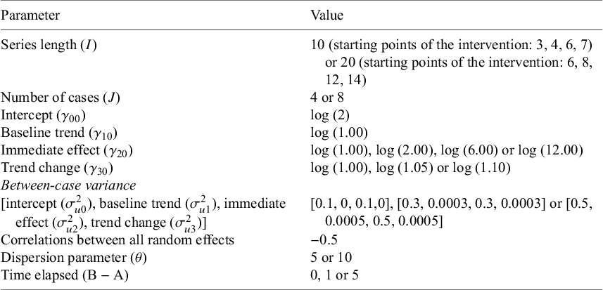

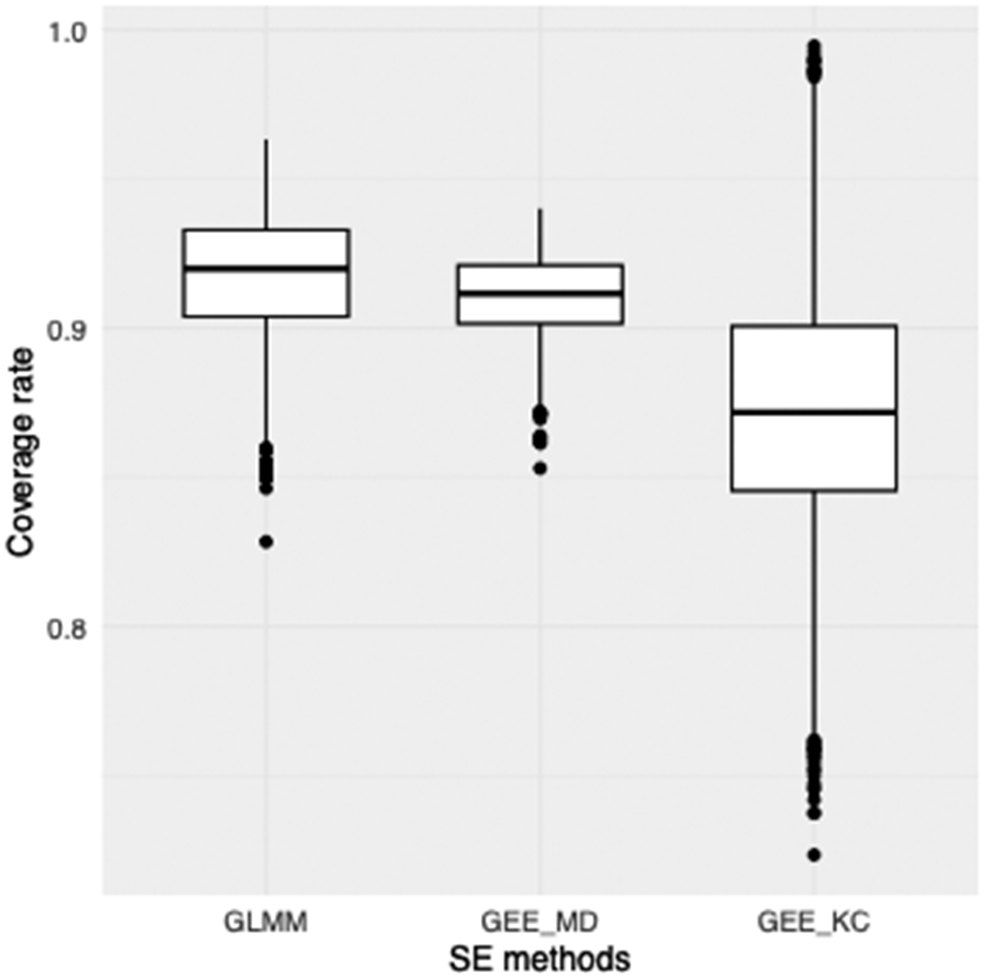


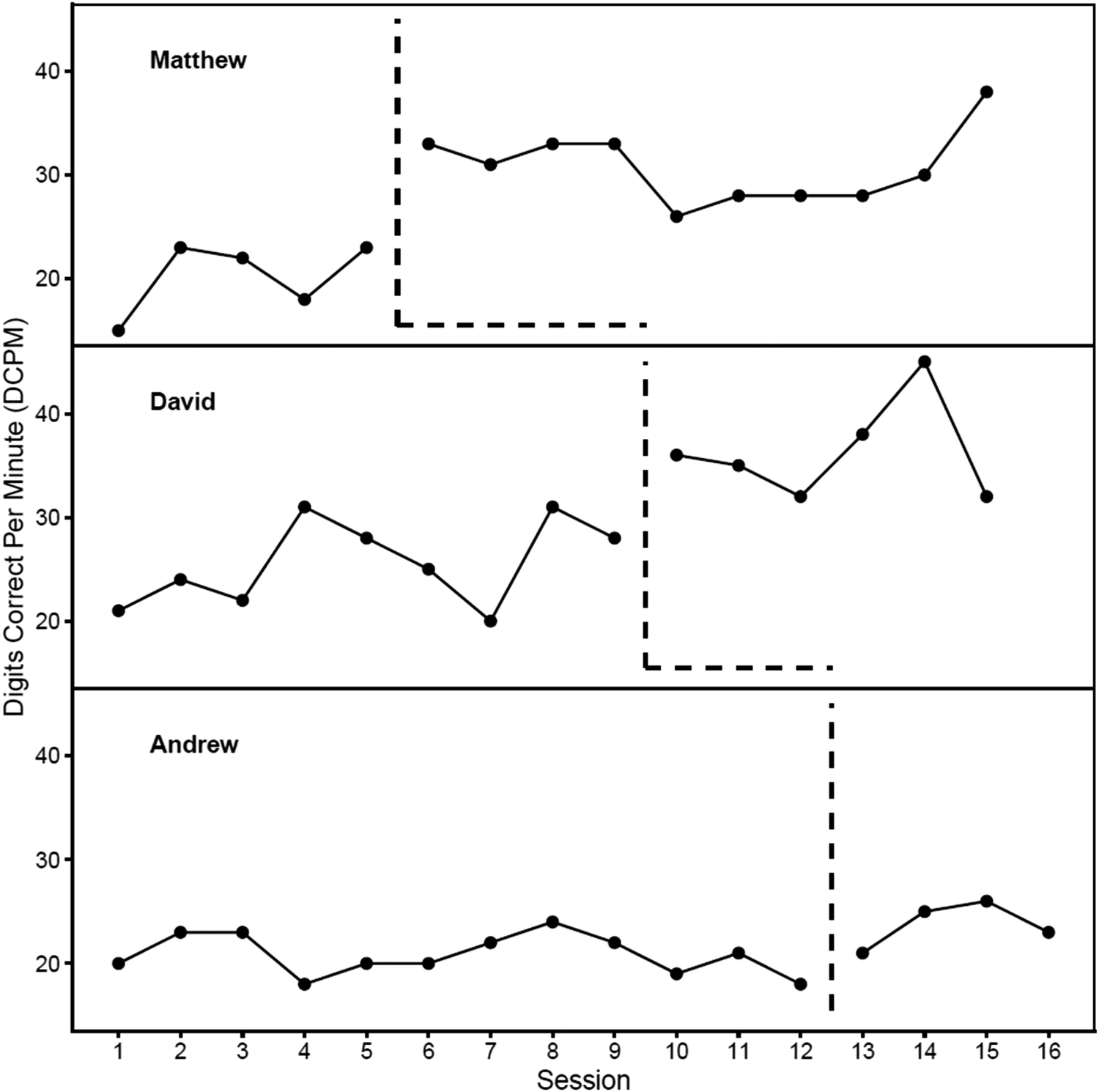
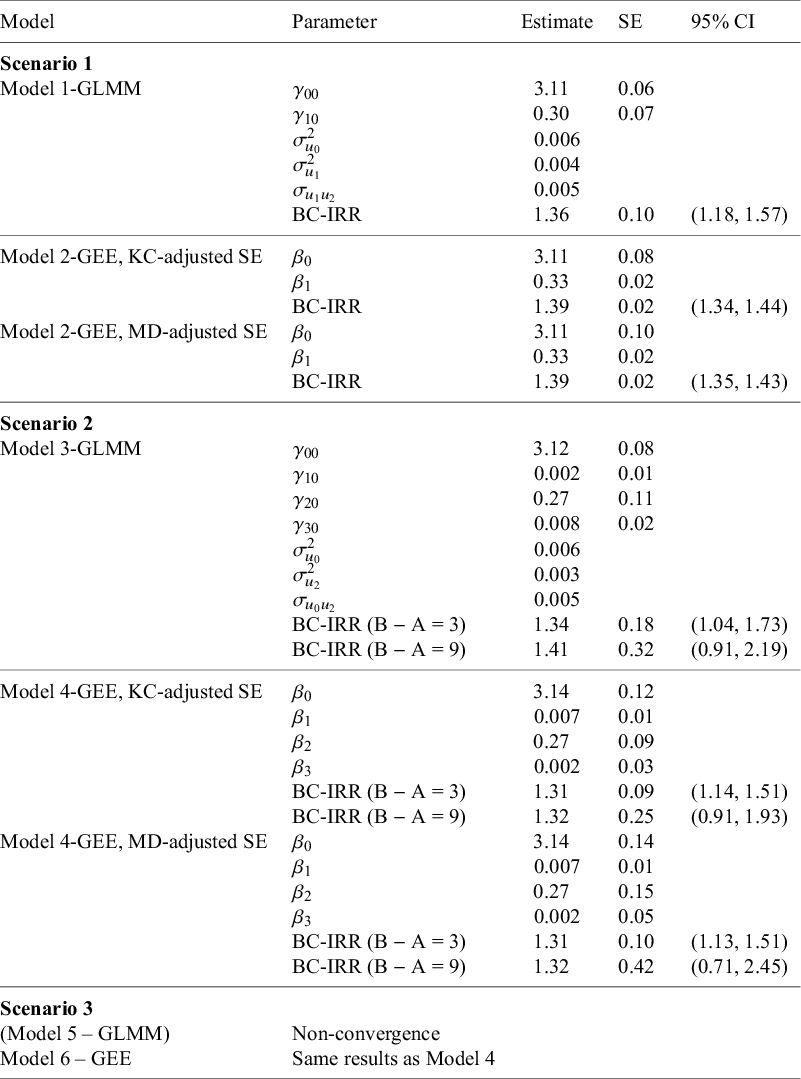

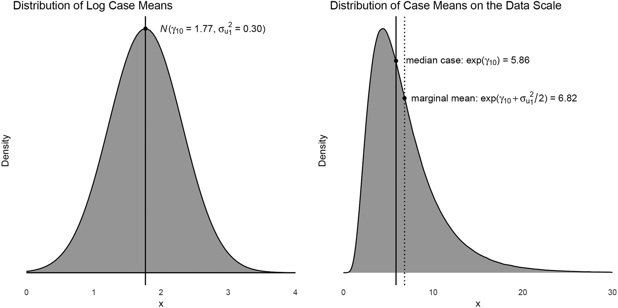

 Open access

