1 Introduction
A tubular flame is a classical configuration used in fundamental studies in combustion science. Their characteristic shape, first observed by Ishizuka (Reference Ishizuka1985) as circular in cross-section and long in the perpendicular direction, distinguishes them from other elementary combustion systems, such as the counterflow, coflow, etc. The most common tubular flame configurations – the swirl type and the counterflow type – have been applied primarily in the analysis of premixed systems. However, after the introduction of non-premixed counterflow tubular systems (Hu et al. Reference Hu, Wang, Pitz and Smooke2007; Wang, Hu & Pitz Reference Wang, Hu and Pitz2007), interest in tubular combustion configurations has increased due to their cylindrical nature, which allows the study of flame curvature effects, making those non-premixed systems suitable for the description of curved flamelets in turbulent combustion modelling (Pitz, Hu & Wang Reference Pitz, Hu and Wang2014; Xuan, Blanquart & Mueller Reference Xuan, Blanquart and Mueller2014). To date, a theoretical model for a non-premixed system equivalent to a premixed swirl-type tubular flame has not been discussed.
The non-premixed counterflow tubular flame is obtained experimentally by using a modified premixed counterflow tubular burner (Mosbacher et al. Reference Mosbacher, Wehrmeyer, Pitz, Sung and Byrd2002). One of the reactants is injected outwards in the radial direction through a porous cylinder along the centre axis (Hu et al. Reference Hu, Wang, Pitz and Smooke2007). An outer contoured nozzle issues the other reactant inwards. As a consequence, the mathematical model of non-premixed tubular systems consists of the same conservation equations used to describe premixed tubular flames (Dixon-Lewis et al. Reference Dixon-Lewis, Giovangigli, Kee, Miller, Rogg, Smooke, Stahl and Warnatz1991; Smooke & Giovangigli Reference Smooke and Giovangigli1991), but with modified boundary conditions to account for the injection of reactants into the chamber from the inner porous cylinder (Wang, Wehrmeyer & Pitz Reference Wang, Wehrmeyer and Pitz2006; Wang et al. Reference Wang, Hu and Pitz2007). Another tubular flame configuration in which the reactants are injected separately, the rapidly mixed burner, has been developed recently (Ishizuka, Motodamari & Shimokuri Reference Ishizuka, Motodamari and Shimokuri2007). This configuration consists of an injection system in which reactants are issued tangentially in a tube through four slits located at its closed end, and a downstream transparent tube allows flame visualization. A Damköhler number analysis suggests that this type of flame can only be established for mixing times shorter than the reaction time, i.e. when the system is actually premixed (Shi, Shimokuri & Ishizuka Reference Shi, Shimokuri and Ishizuka2013).
The majority of the studies on tubular flames are limited to the analysis of systems with fuel in the gas phase. One of the few exceptions is the liquid film combustor (Sirignano, Pham & Dunn-Rankin Reference Sirignano, Pham and Dunn-Rankin2002). The liquid film combustor takes advantage of the fact that for miniature systems a condensed fuel layer can offer a surface area for vaporization as high as in vaporizing sprays (Dunn-Rankin Reference Dunn-Rankin, Ishiuka, Dunn-Rankin and Pitz2013). In this configuration liquid fuel is injected tangentially onto a tube wall, creating a thin film on its surface. A swirling air flow is introduced from the closed end of the tube through a swirl generator (Giani & Dunn-Rankin Reference Giani and Dunn-Rankin2013). The injection of swirling air creates a rotational movement of the flow field which helps to spread the fuel and stabilize the film on the combustor inner surface (Pham, Dunn-Rankin & Sirignano Reference Pham, Dunn-Rankin and Sirignano2007). A mathematical model for the system considering unity Lewis numbers was developed to describe theoretically the combustion process in the liquid film burner (Sirignano, Stanchi & Imaoka Reference Sirignano, Stanchi and Imaoka2005). Perturbations were used to account for effects of swirl-induced flow, vaporization-induced flow and gas expansion on an undisturbed plug flow. For the case of a parabolic velocity profile, the combination of these effects was not taken into account.
The combustion of liquid fuels requires a phase change before mixing, and hence is much more complex when compared to combustion of gaseous fuels. In the combustion of condensed fuels the flame is located in the gas phase, and a portion of the heat generated by the chemical reaction is conducted towards the liquid phase to provide the latent heat needed to vaporize the fuel (Spalding Reference Spalding1950). At the same time, the gas phase reaction can be accompanied by a number of complicating parameters such as the pyrolysis of the fuel, formation of condensed products, heterogeneous reactions, phase transitions, etc., which, consequently, creates difficulties in developing theoretical models (Namyatov et al. Reference Namyatov, Minaev, Babkin, Bunev and Korzhavin2000). As a result, the mechanisms involved in the combustion of liquid and gaseous fuels in a tubular system are very distinct, even though the configurations are similar. However, notwithstanding the complications involved in their analysis, most of the fuels used for propulsion are in the liquid phase, making it necessary to develop tubular flame systems where condensed fuels can be applied.
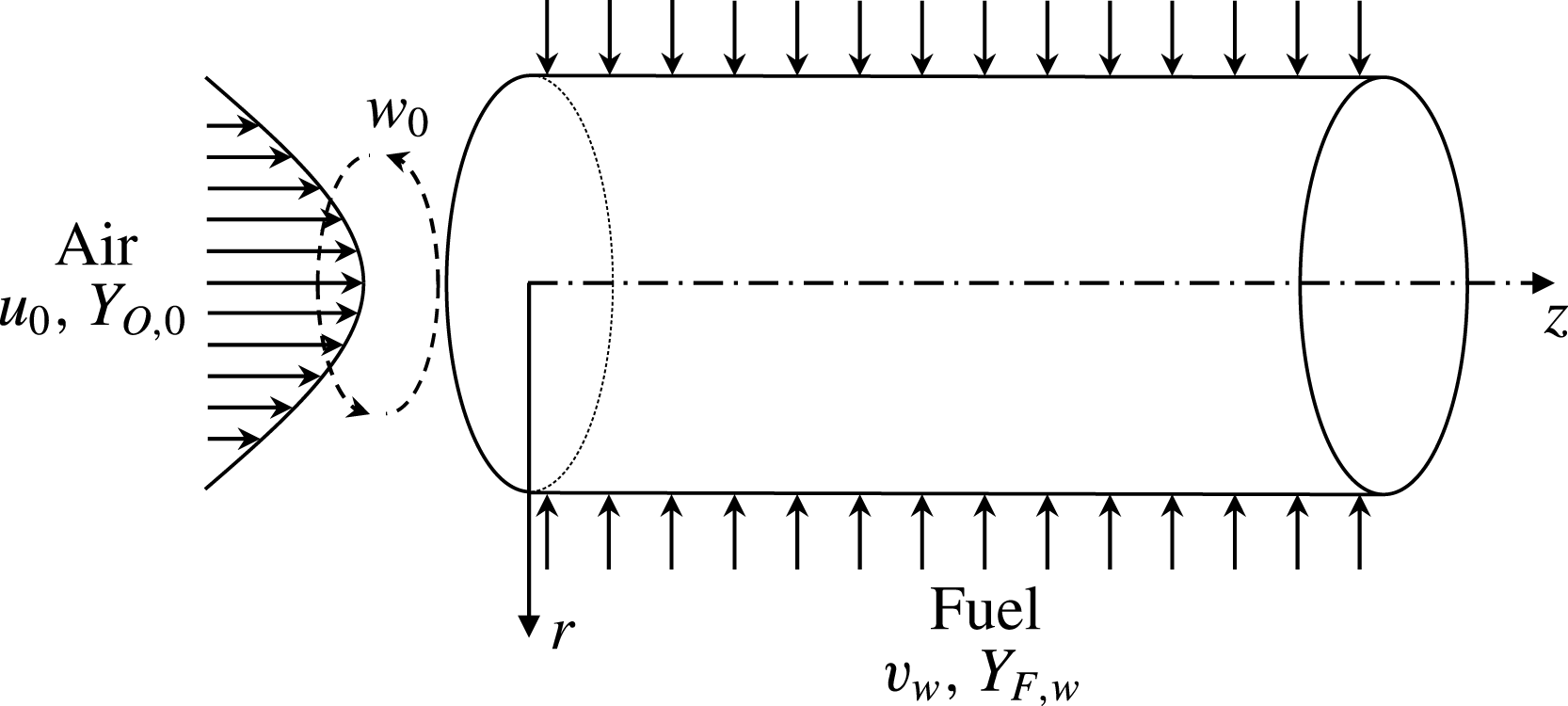
The non-premixed swirl-type concept is based on radial injection of fuel, and takes advantage of the advances in liquid fuel film and classical tubular flame burners. In this new configuration, illustrated in figure 1, instead of developing a layer of liquid on the inner surface of the combustion chamber, the condensed fuel is injected through the burner walls, which are permeable. The condensed fuel vaporizes thereby becoming the gaseous fuel source for the chemical reaction with the swirling air that is injected axially. The flame is located in the combustion chamber between the burner walls and the exhaust gas. This new configuration, as well as the liquid film burner, are potential alternatives to the systems that, otherwise, would be limited by the difficulties inherent to the atomization of condensed fuel. At the same time, the condensed fuel can offer protection from heat losses and quenching since the temperature of the walls does not exceed the boiling point of the fuel.
Representation of the physical system.

The mathematical description of the system is based on two classical models for pipes flows. The fuel injection is described by the theory of laminar pipe flows with porous walls. The solution of the Navier–Stokes equations for fully developed flows in channels with rectangular permeable walls was first presented by Berman (Reference Berman1953). A constant flow velocity inside the porous wall was assumed, and the conservation equations transformed using a streamfunction defined in terms of a similarity variable. The analysis was extended to circular pipe flows by Yuan & Finkelstein (Reference Yuan and Finkelstein1955), and was extensively investigated in several studies by a number of groups (Sellars Reference Sellars1955; Eckert, Donoughe & Moore Reference Eckert, Donoughe and Moore1957; Berman Reference Berman1958; White Reference White1962; Terrill Reference Terrill1964; Terrill & Thomas Reference Terrill and Thomas1969). The study of rotating porous pipes was also considered, but with the assumption that swirl velocity was constant along the pipe (Prager Reference Prager1964; Terrill Reference Terrill1967; Terrill & Thomas Reference Terrill and Thomas1973; Banks & Zaturska Reference Banks and Zaturska1996). Details of the published work on laminar flows in porous ducts have been presented in an in-depth review (Chellam et al. Reference Chellam, Wiesner, Dawson and Brown1995). The theory for laminar pipe flows with porous walls was extended by Yuan & Finkelstein (Reference Yuan and Finkelstein1958) for the investigation of the heat transfer problem for a steady fully developed laminar flow developed by Graetz (Reference Graetz1882). The conservation equations for energy and species were modified by the introduction of velocity components from the solution of the momentum equations for laminar pipe flows with porous walls. Their work was followed by a number of investigations that accounted for injection and extraction of mass (Kinney Reference Kinney1968), different boundary conditions (Raithby Reference Raithby1971), mass transfer cooling (Peng & Yuan Reference Peng and Yuan1965) and internal heat sources (Eroshenko, Zaichik & Rabovskii Reference Eroshenko, Zaichik and Rabovskii1980). The analysis of the flow field in the system is performed on the basis of the theory developed for swirling laminar flows. Among early relevant analytical descriptions of this type of flow are those of Collatz & Görtler (Reference Collatz and Görtler1954) and Talbot (Reference Talbot1954), who analysed analytically the decay of swirl in tubes with impermeable walls. Collatz & Görtler (Reference Collatz and Görtler1954) presented a solution for the tangential velocity field, but it did not account for concomitant disturbances of the axial and radial velocity fields. On the other hand, Talbot (Reference Talbot1954) presented a study in which the disturbances of the axial and radial velocities were considered using a momentum integral equation. Deka (Reference Deka1963, Reference Deka1966) and Lavan, Nielsen & Fejer (Reference Lavan, Nielsen and Fejer1969) obtained an equivalent solution to problems in which the downstream section of the tube rotates and the upstream region is stationary by employing integral transforms. Kreith & Sonju (Reference Kreith and Sonju1965) extended the analysis to study the swirl decay in turbulent flows, modifying the swirl equations through the introduction of an eddy diffusivity term. Kinney & Sparrow (Reference Kinney and Sparrow1970) extended the analytical solution of the swirl decay in tubes by combining it with the theory of laminar pipe flows with porous walls to account for tubes with surface mass transfer. The assumption in their analysis is similar to the ones from Deka (Reference Deka1963, Reference Deka1966) and Lavan et al. (Reference Lavan, Nielsen and Fejer1969), and consisted of a porous pipe with a downstream rotating porous wall where the swirl is generated and an upstream stationary permeable pipe where mass is injected (or removed) and the swirl decays. Lee, Ou & Chen (Reference Lee, Ou and Chen1987) used the same framework as Talbot (Reference Talbot1954) to obtain the velocity field for the growing swirl in a rotating tube. The resultant mixing induced by the fluid flow in the presence of molecular diffusion and chemical reactions was characterized.
The analysis herein presents an effort to combine the effect of swirl decay in tubes with heat and mass transfer in laminar pipe flows with porous walls. Although considered separately in the prior work cited above, these effects have not been combined in the analysis of reacting nor non-reacting flows in pipes. The model is used to predict important flame characteristics in a non-premixed system, in which oxidizer is introduced through a swirling flow from one end and fuel is supplied from the walls of the burner. The conservation equations for energy and species are transformed using the Shvab–Zel’dovich approach, so that the solution methods used in the study of convective heat and mass transfer in confined flows can also be applied. The model can provide theoretical support and general design guidelines to the development of non-premixed swirl-type tubular systems.
2 Theoretical model
The combustion process in non-premixed flames is controlled by the rate at which fuel and oxidizer are brought together in proper proportions. In the Burke–Schumann limit, the chemical reactions are described by an irreversible infinitely fast conversion of reactants into stable products. That creates a very thin exothermic reaction zone at high temperature and with high concentration of combustion products, where stoichiometric mixing of fuel (F) and oxidizer (
 $\text{O}_{2}$
) takes place. As a consequence, fuel and oxidizer sides are separated by the reaction sheet. The combustion process is represented by
 $$\begin{eqnarray}\text{F}+s\text{O}_{2}\longrightarrow s_{\text{CO}_{2}}\text{CO}_{2}+s_{\text{H}_{2}\text{O}}\text{H}_{2}\text{O}.\end{eqnarray}$$
The overall reaction (I) represents with good accuracy the chemical processes when the concentrations of major species outnumber significantly the minor species. In the formulation
 $s$
,
 $s_{\text{CO}_{2}}$
,
 $s_{\text{H}_{2}\text{O}}$
are, respectively, the mass of oxygen consumed, and the mass of carbon dioxide (
 $\text{CO}_{2}$
) and water vapour (
 $\text{H}_{2}\text{O}$
) produced, for which,
 $1+s=s_{\text{CO}_{2}}+s_{\text{H}_{2}\text{O}}$
. The dimensionless axisymmetric steady-state conservation equations of mass, momentum in the axial, radial and tangential directions, energy, and species for the gas phase, considering it an incompressible flow with constant physical properties throughout the whole domain, are given by
 $$\begin{eqnarray}\displaystyle & \displaystyle \frac{1}{Re_{0}}\frac{\unicode[STIX]{x2202}u}{\unicode[STIX]{x2202}z}+\frac{1}{r}\frac{\unicode[STIX]{x2202}}{\unicode[STIX]{x2202}r}(rv)=0, & \displaystyle\end{eqnarray}$$
 $$\begin{eqnarray}\displaystyle & \displaystyle \frac{u}{Re_{0}}\frac{\unicode[STIX]{x2202}u}{\unicode[STIX]{x2202}z}+v\frac{\unicode[STIX]{x2202}u}{\unicode[STIX]{x2202}r}=-\frac{1}{Re_{0}}\frac{\unicode[STIX]{x2202}p}{\unicode[STIX]{x2202}z}+\frac{2}{Re_{0}}\left[\frac{1}{r}\frac{\unicode[STIX]{x2202}}{\unicode[STIX]{x2202}r}\left(r\frac{\unicode[STIX]{x2202}u}{\unicode[STIX]{x2202}r}\right)+\frac{1}{Re_{0}^{2}}\frac{\unicode[STIX]{x2202}^{2}u}{\unicode[STIX]{x2202}z^{2}}\right], & \displaystyle\end{eqnarray}$$
 $$\begin{eqnarray}\displaystyle & \displaystyle \frac{u}{Re_{0}}\frac{\unicode[STIX]{x2202}v}{\unicode[STIX]{x2202}z}+v\frac{\unicode[STIX]{x2202}v}{\unicode[STIX]{x2202}r}-\frac{w^{2}}{r}=-\frac{\unicode[STIX]{x2202}p}{\unicode[STIX]{x2202}r}+\frac{2}{Re_{0}}\left[\frac{1}{r}\frac{\unicode[STIX]{x2202}}{\unicode[STIX]{x2202}r}\left(r\frac{\unicode[STIX]{x2202}v}{\unicode[STIX]{x2202}r}\right)-\frac{v}{r^{2}}+\frac{1}{Re_{0}^{2}}\frac{\unicode[STIX]{x2202}^{2}v}{\unicode[STIX]{x2202}z^{2}}\right], & \displaystyle\end{eqnarray}$$
 $$\begin{eqnarray}\displaystyle & \displaystyle \frac{u}{Re_{0}}\frac{\unicode[STIX]{x2202}w}{\unicode[STIX]{x2202}z}+v\frac{\unicode[STIX]{x2202}w}{\unicode[STIX]{x2202}r}+\frac{vw}{r}=\frac{2}{Re_{0}}\left[\frac{1}{r}\frac{\unicode[STIX]{x2202}}{\unicode[STIX]{x2202}r}\left(r\frac{\unicode[STIX]{x2202}w}{\unicode[STIX]{x2202}r}\right)-\frac{w}{r^{2}}+\frac{1}{Re_{0}^{2}}\frac{\unicode[STIX]{x2202}^{2}w}{\unicode[STIX]{x2202}z^{2}}\right], & \displaystyle\end{eqnarray}$$
 $$\begin{eqnarray}\displaystyle & \displaystyle \frac{u}{Re_{0}}\frac{\unicode[STIX]{x2202}Y_{k}}{\unicode[STIX]{x2202}z}+v\frac{\unicode[STIX]{x2202}Y_{k}}{\unicode[STIX]{x2202}r}=\frac{2}{Pe_{0}}\left[\frac{1}{r}\frac{\unicode[STIX]{x2202}}{\unicode[STIX]{x2202}r}\left(r\frac{\unicode[STIX]{x2202}Y_{k}}{\unicode[STIX]{x2202}r}\right)+\frac{1}{Re_{0}^{2}}\frac{\unicode[STIX]{x2202}^{2}Y_{k}}{\unicode[STIX]{x2202}z^{2}}\right]-S_{k}{\dot{m}}, & \displaystyle\end{eqnarray}$$
 $$\begin{eqnarray}\displaystyle & \displaystyle \frac{u}{Re_{0}}\frac{\unicode[STIX]{x2202}T}{\unicode[STIX]{x2202}z}+v\frac{\unicode[STIX]{x2202}T}{\unicode[STIX]{x2202}r}=\frac{2}{Pe_{0}}\left[\frac{1}{r}\frac{\unicode[STIX]{x2202}}{\unicode[STIX]{x2202}r}\left(r\frac{\unicode[STIX]{x2202}T}{\unicode[STIX]{x2202}r}\right)+\frac{1}{Re_{0}^{2}}\frac{\unicode[STIX]{x2202}^{2}T}{\unicode[STIX]{x2202}z^{2}}\right]+\unicode[STIX]{x1D6FE}(1+S){\dot{m}}, & \displaystyle\end{eqnarray}$$
where
 $u\equiv \hat{u} /\hat{U} _{0}$
,
 $v\equiv \hat{v}/\hat{U} _{0}$
and
 $w\equiv {\hat{w}}/\hat{U} _{0}$
are the velocity components in the axial, radial and circumferential directions scaled by the average velocity at the inlet
 $\hat{U} _{0}$
. The other dependent variables,
 $p\equiv \hat{p}/\hat{\unicode[STIX]{x1D70C}}\hat{U} _{0}^{2}$
,
 $T\equiv (\hat{T}-\hat{T}_{0})/\hat{T}_{0}$
and
 $Y_{k}\equiv {\hat{Y}}_{k}/{\hat{Y}}_{k,ref}$
are pressure, temperature and mass fractions of species
 $k$
, respectively, for
 $k=\text{F}$
, O,
 $\text{CO}_{2}$
or
 $\text{H}_{2}\text{O}$
, scaled by their respective reference values. The parameter
 $\hat{T}_{0}$
represents the temperature at the air inlet and
 $\hat{\unicode[STIX]{x1D70C}}$
denotes the gas density. The independent variables
 $r\equiv \hat{r}/\hat{r}_{w}$
and
 $z\equiv \hat{z}/\hat{r}_{w}Re_{0}$
are scaled by the internal radius of the tube,
 $\hat{r}_{w}$
, and the Reynolds number,
 $Re_{0}\equiv 2\hat{r}_{w}\hat{U} _{0}/\hat{\unicode[STIX]{x1D708}}$
, where
 $\hat{\unicode[STIX]{x1D708}}$
is the kinematic viscosity. The term
 ${\dot{m}}\equiv \hat{r}_{w}\hat{{\dot{m}}}/\hat{\unicode[STIX]{x1D70C}}\hat{U} _{0}$
represents the rate of consumption of fuel mass. The flows considered are laminar with large axial Reynolds numbers
 $Re_{0}$
. Therefore, diffusion in the streamwise direction is negligible since it scales with
 $1/Re_{0}^{2}$
. Besides the condition of equal diffusion speed between all species, unity Lewis numbers are assumed, i.e. equal mass and heat diffusion, denoted by
 $\hat{{\mathcal{D}}}$
and
 $\hat{\unicode[STIX]{x1D6FC}}$
, respectively. The Péclet number is defined as
 $Pe_{0}\equiv 2\hat{r}_{w}\hat{U} _{0}/\hat{\unicode[STIX]{x1D6FC}}$
. The stoichiometric mass ratios are defined as
 $S\equiv s{\hat{Y}}_{\text{F},w}/{\hat{Y}}_{\text{O},0}$
,
 $\text{S}_{\text{H}_{2}\text{O}}\equiv s_{\text{H}_{2}\text{O}}{\hat{Y}}_{\text{F},w}$
and
 $\text{S}_{\text{CO}_{2}}\equiv s_{\text{CO}_{2}}{\hat{Y}}_{\text{F},w}$
and the heat release
 $\unicode[STIX]{x1D6FE}\equiv \hat{q}_{c}{\hat{Y}}_{\text{F},w}/{\hat{c}}_{p}\hat{T}_{0}(S+1)$
, where
 $\hat{q}_{c}$
is the amount of heat released per amount of fuel burnt and
 ${\hat{c}}_{p}$
is the specific heat at constant pressure of the gas phase. Small Mach number is assumed for the flow. Buoyancy, heat transport by radiation, Soret and Dufour effects are neglected in the analysis. Fick’s law is used to describe diffusion velocities of species. Assuming no penetration of other species at the liquid–vapour interface, Stefan convection and diffusion on the gas side and the convection on the liquid side are related by
 $$\begin{eqnarray}v_{w^{-}}Y_{k,w^{-}}-\left.\frac{2}{Pe_{0}}\frac{\unicode[STIX]{x2202}Y_{k}}{\unicode[STIX]{x2202}r}\right|_{r=1^{-}}=v_{w^{-}}Y_{\text{F},l}\unicode[STIX]{x1D6FF}_{k,\text{F}},\end{eqnarray}$$
where
 $\unicode[STIX]{x1D6FF}$
is the delta function and
 $Y_{\text{F},l}$
is the mass fraction of fuel in the condensed phase. Purely inward radial flow is assumed inside the porous medium, which means that we consider the flow inside the porous matrix not affected by the flow in the tube. From mass conservation, the radial velocity
 $v_{w^{-}}$
at the internal radius of the tube is related to the fuel velocity in the condensed phase according to
 $v_{w^{-}}=\unicode[STIX]{x1D711}\unicode[STIX]{x1D70C}_{l}v_{w^{+}}$
, in which
 $\unicode[STIX]{x1D70C}_{l}\equiv \hat{\unicode[STIX]{x1D70C}}_{l}/\hat{\unicode[STIX]{x1D70C}}$
is the liquid fuel density and
 $\unicode[STIX]{x1D711}$
is the porosity of the permeable tube walls. The superscripts
 $-$
and
 $+$
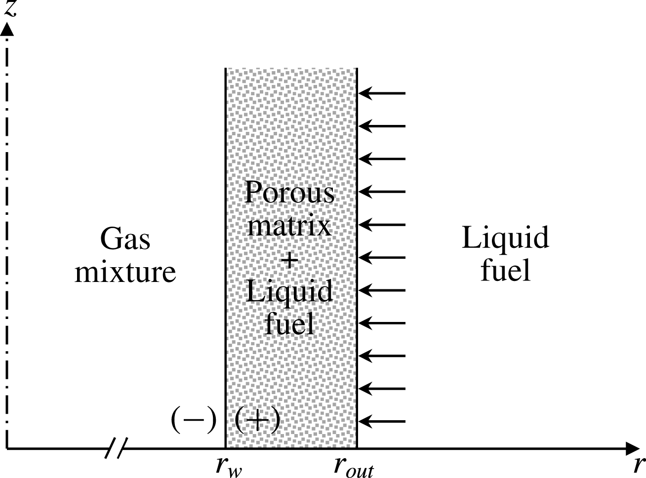
denote the gas and liquid sides at the tube wall, respectively, as shown in figure 2. From a first law analysis at the interface, assuming it to be non-reacting,
 $$\begin{eqnarray}\left.\frac{2}{Pe_{0}}\frac{\unicode[STIX]{x2202}T}{\unicode[STIX]{x2202}r}\right|_{r=1^{-}}=\left.\frac{\hat{\unicode[STIX]{x1D70C}}_{l}{\hat{c}}_{l}}{\hat{\unicode[STIX]{x1D70C}}{\hat{c}}_{p}}\frac{2}{Pe_{m}}\frac{\unicode[STIX]{x2202}T}{\unicode[STIX]{x2202}r}\right|_{r=1^{+}}+v_{w^{-}}L,\end{eqnarray}$$
where
 $L\equiv \hat{L}/{\hat{c}}_{p}\hat{T}_{0}$
, in which
 $\hat{L}$
is the latent heat of vaporization. The Péclet number on the porous medium side is defined as
 $Pe_{m}\equiv 2\hat{r}_{w}\hat{U} _{0}/\hat{\unicode[STIX]{x1D6FC}}_{m}$
, where
 $\hat{\unicode[STIX]{x1D6FC}}_{m}\equiv \hat{\unicode[STIX]{x1D705}}_{m}/(\hat{\unicode[STIX]{x1D70C}}{\hat{c}})_{l}$
is the thermal diffusivity of the porous medium, and
 $\hat{\unicode[STIX]{x1D705}}_{m}\equiv \unicode[STIX]{x1D711}\hat{\unicode[STIX]{x1D705}}_{l}+(1-\unicode[STIX]{x1D711})\hat{\unicode[STIX]{x1D705}}_{s}$
, in which
 $\hat{\unicode[STIX]{x1D705}}$
is the thermal conductivity and
 ${\hat{c}}$
the specific heat capacity. The subscripts
 $l$
and
 $s$
denote the liquid and solid phases, respectively.
Representation of the wall interface.

The fuel is heated from the injection temperature,
 $T=0$
, to a state close to its boiling point
 $T=T_{b}$
. The amount of heat necessary for that to happen is supplied by the hot gas in the combustion chamber. Thus, some of the heat generated by the reacting flow is used to vaporize the fuel and the remainder is conducted into the permeable wall. It is assumed that the porous wall is an isotropic medium where radiative effects, viscous dissipation and work done by pressure changes are negligible, that there is local thermal equilibrium between the solid and fluid phases, and that heat conduction in both phases takes place in parallel such that there is no heat transfer from one phase to the other (Nield & Bejan Reference Nield and Bejan2013). Moreover, considering the permeable wall consisting of an interior region at uniform temperature,
 $T_{0}$
, and a thin layer at the wall surface temperature,
 $T_{w}$
, and neglecting the axial components of the fluid flow with respect to the terms in the radial direction, the heat conducted to the liquid phase is given as
 $$\begin{eqnarray}\frac{2}{Pe_{0}}\left.\frac{\unicode[STIX]{x2202}T}{\unicode[STIX]{x2202}r}\right|_{r=1^{-}}=v_{w^{-}}L_{eff},\end{eqnarray}$$
in which the effective latent heat of vaporization is defined as
 $L_{eff}\equiv c_{l}T_{w}+L$
. For simplicity the wall surface temperature is assumed to be equal to the boiling point of the fuel, i.e.
 $T_{w}=T_{b}$
. This condition prescribes both the temperature and the mass fraction at the walls. As a consequence, mass and energy fluxes at the walls are allowed to vary in the axial direction. In order to further simplify the analysis, an average value
 $V_{w}$
is used in the conservation equations as an approximation to the absolute value of the velocity at the wall
 $|v_{w^{-}}|$
. The term
 $V_{w}$
becomes an eigenvalue of the problem, specified through the imposition of the boundary conditions. Its value is determined by considering an estimate value
 $V_{w}$
, which is corrected until it equals the average of
 $|v_{w^{-}}|$
, obtained by substituting the solution for
 $T$
into (2.9). The boundary conditions at the axis of symmetry, internal surface of the tube, and at the inlet are given as
 $$\begin{eqnarray}\displaystyle & \displaystyle \frac{\unicode[STIX]{x2202}u}{\unicode[STIX]{x2202}r}=v=w=\frac{\unicode[STIX]{x2202}Y_{k}}{\unicode[STIX]{x2202}r}=\frac{\unicode[STIX]{x2202}T}{\unicode[STIX]{x2202}r}=0,\quad r=0, & \displaystyle\end{eqnarray}$$
 $$\begin{eqnarray}\displaystyle & \displaystyle u=v+V_{w}=w=T-T_{b}=Y_{\text{F}}-Y_{\text{F},w}=Y_{\text{O}}=0,\quad r=1, & \displaystyle\end{eqnarray}$$
 $$\begin{eqnarray}\displaystyle & \displaystyle u-u_{0}=v=w-w_{0}=T=Y_{\text{F}}=Y_{\text{O}}-1=0,\quad z=0. & \displaystyle\end{eqnarray}$$
In this analysis, a swirl velocity
 $w_{0}$
, with a maximum intensity
 $W_{0}\equiv {\hat{W}}_{0}/\hat{U} _{0}$
, is imposed at the flow inlet satisfying the condition
 $W_{0}\ll 1$
. Therefore, the swirl component in the flow field can be considered as a perturbation, which allows the use of series expansion to solve the problem. The condition of a long tube with a very small ratio of radius to length is considered. The flow rate of oxidant at
 $z=0$
is limited to laminar Reynolds number
 $Re_{0}$
conditions. However, the amount of fuel delivered to the system can be as large as the tube length permits, which, at some position along the tube, can create excessively rich regions that result in local flame extinction. Under some conditions, the flame can reignite and maintain itself for a certain length, establishing ‘flame streets’ as described by Mohan & Matalon (Reference Mohan and Matalon2017). This combustion regime will not be included in the analysis.
The linear combination of energy and mass fraction conservation equations eliminates the reaction terms through the introduction of two conserved scalars, namely, the mixture fraction
 $Z$
, and the excess-enthalpy
 $H$
(Liñán, Vera & Sánchez Reference Liñán, Vera and Sánchez2015). The conserved scalars can be further simplified because of the assumption of unity Lewis numbers. In that case, the conservation equations for the conserved scalars are given, respectively, as
 $$\begin{eqnarray}\displaystyle & \displaystyle \frac{u}{Re_{0}}\frac{\unicode[STIX]{x2202}Z}{\unicode[STIX]{x2202}z}+v\frac{\unicode[STIX]{x2202}Z}{\unicode[STIX]{x2202}r}-\frac{2}{Pe_{0}}\left[\frac{1}{r}\frac{\unicode[STIX]{x2202}}{\unicode[STIX]{x2202}r}\left(r\frac{\unicode[STIX]{x2202}Z}{\unicode[STIX]{x2202}r}\right)\right]=0, & \displaystyle\end{eqnarray}$$
 $$\begin{eqnarray}\displaystyle & \displaystyle \frac{u}{Re_{0}}\frac{\unicode[STIX]{x2202}H}{\unicode[STIX]{x2202}z}+v\frac{\unicode[STIX]{x2202}H}{\unicode[STIX]{x2202}r}-\frac{2}{Pe_{0}}\left[\frac{1}{r}\frac{\unicode[STIX]{x2202}}{\unicode[STIX]{x2202}r}\left(r\frac{\unicode[STIX]{x2202}H}{\unicode[STIX]{x2202}r}\right)\right]=0, & \displaystyle\end{eqnarray}$$
in which the mixture fraction and the excess enthalpy are defined, respectively, as (Liñán et al. Reference Liñán, Vera and Sánchez2015)
 $$\begin{eqnarray}\displaystyle & \displaystyle Z\equiv (SY_{\text{F}}-Y_{\text{O}}+1)/(S+1), & \displaystyle\end{eqnarray}$$
 $$\begin{eqnarray}\displaystyle & \displaystyle H\equiv T+\unicode[STIX]{x1D6FE}(S+1)(Y_{\text{O}}-1)/S. & \displaystyle\end{eqnarray}$$
At the flame front, the concentrations of fuel
 $Y_{\text{F}}$
and oxygen
 $Y_{\text{O}}$
go to zero and the flame position
 $r_{f}$
can be determined by
 $$\begin{eqnarray}Z_{f}=1/(S+1)\end{eqnarray}$$
and the peak flame temperature can be obtained as (Sauer, Leiroz & Colaço Reference Sauer, Leiroz and Colaço2012; Liñán et al. Reference Liñán, Vera and Sánchez2015)
 $$\begin{eqnarray}T_{f}=T_{0}+\unicode[STIX]{x1D6FE}Y_{\text{F},w}+\frac{T_{w}-T_{0}}{S+1}.\end{eqnarray}$$
The boundary conditions for (2.11) and (2.12) are obtained by combining (2.10), (2.13) and (2.14):
 $$\begin{eqnarray}\displaystyle & \displaystyle \frac{\unicode[STIX]{x2202}Z}{\unicode[STIX]{x2202}r}=\frac{\unicode[STIX]{x2202}H}{\unicode[STIX]{x2202}r}=0,\quad r=0, & \displaystyle\end{eqnarray}$$
 $$\begin{eqnarray}\displaystyle & \displaystyle H-H_{w}=Z-Z_{w}=0,\quad r=1, & \displaystyle\end{eqnarray}$$
 $$\begin{eqnarray}\displaystyle & \displaystyle H=Z=0,\quad \tilde{z}=0. & \displaystyle\end{eqnarray}$$
 $$\begin{eqnarray}\displaystyle & \displaystyle \left.\frac{2}{Pe_{0}}\frac{\unicode[STIX]{x2202}Z}{\unicode[STIX]{x2202}r}\right|_{r=1}=-\frac{Sv_{w^{-}}(1-Y_{\text{F},w})}{(S+1)}, & \displaystyle\end{eqnarray}$$
 $$\begin{eqnarray}\displaystyle & \displaystyle \frac{2}{Pe_{0}}\left.\frac{\unicode[STIX]{x2202}H}{\unicode[STIX]{x2202}r}\right|_{r=1}=v_{w^{-}}L_{eff}. & \displaystyle\end{eqnarray}$$
2.1 Flow field
The model is based on the theory of internal laminar swirling flows with surface mass and heat transfer. Due to the swirling nature of the gas flow, the equations of motion are represented in a form that allows the rotating field to be taken into account by superimposing a laminar swirl flow on a Poiseuille flow in a straight pipe. The flow through the tube is two-dimensional, axisymmetric, laminar and the physical properties do not vary with temperature. The velocity components are represented in the form (Deka Reference Deka1963)
 $$\begin{eqnarray}\displaystyle & \displaystyle u=u^{o}(r,z)+\unicode[STIX]{x1D700}^{2}u^{\ast }(r,z)+O(\unicode[STIX]{x1D700}^{3}), & \displaystyle\end{eqnarray}$$
 $$\begin{eqnarray}\displaystyle & \displaystyle v=v^{o}(r)+\unicode[STIX]{x1D700}^{2}v^{\ast }(r,z)+O(\unicode[STIX]{x1D700}^{3}), & \displaystyle\end{eqnarray}$$
 $$\begin{eqnarray}\displaystyle & \displaystyle w=\unicode[STIX]{x1D700}w^{\ast }(r,z)+O(\unicode[STIX]{x1D700}^{2}), & \displaystyle\end{eqnarray}$$
 $o$
represents
 $O(\unicode[STIX]{x1D700}^{0})$
terms, i.e. velocities of undisturbed flow field and the velocity downstream, where perturbations have dissipated and the velocity field has attained a fully developed profile. Since axisymmetric conditions are imposed on the problem, the circumferential velocity perturbation
 $w^{\ast }$
has an influence on the species and temperature field through the other velocity components,
 $u$
and
 $v$
. By considering
 $w$
as a perturbation of
 $O(\unicode[STIX]{x1D700})$
, from (2.3), it is observed that its effect is to induce a
 $O(\unicode[STIX]{x1D700}^{2})$
perturbation to the velocity components
 $u$
and
 $v$
. The model does not account for perturbations other than the one due to the swirl, therefore
 $O(\unicode[STIX]{x1D700})$
terms are not included in the axial and radial velocities expansions in (2.19). The term
 $W_{0}$
is assumed as the magnitude of the swirl perturbation. Consequently, in (2.19), for
 $W_{0}\ll 1$
,
 $\unicode[STIX]{x1D700}=W_{0}$
. The swirl angle
 $\unicode[STIX]{x1D703}$
is related to
 $W_{0}$
by
 $$\begin{eqnarray}W_{0}=\tan \unicode[STIX]{x1D703}.\end{eqnarray}$$
The procedure employed to obtain the velocity components of the flow field in this section follows closely the derivation presented by Kinney & Sparrow (Reference Kinney and Sparrow1970).
2.1.1 Fully developed velocity profile
With the assumption of steady burning, the mass flow rate of fuel from the porous walls is constant. In the fully developed region of such flows, it has been shown, from the overall mass conservation, that the flow field can be described in terms of the streamfunction (Yuan & Finkelstein Reference Yuan and Finkelstein1955) as
 $$\begin{eqnarray}\unicode[STIX]{x1D6F9}(r,z)={\textstyle \frac{1}{2}}rG(r)U(z),\end{eqnarray}$$
in which
 $G(r)$
is an unspecified function of
 $r$
, and the function
 $U(z)=(1+2Re_{w}z)$
is the flow local mean axial velocity (Collatz & Görtler Reference Collatz and Görtler1954), where the wall injection Reynolds number is defined as
 $$\begin{eqnarray}Re_{w}\equiv 2\hat{r}_{w}\hat{V}_{w}/\hat{\unicode[STIX]{x1D708}}=V_{w}Re_{0}.\end{eqnarray}$$
The velocity components in the axial and radial directions can be written, respectively, as (Berman Reference Berman1958)
 $$\begin{eqnarray}\displaystyle & \displaystyle u^{o}(r,z)=U(z)F(r), & \displaystyle\end{eqnarray}$$
 $$\begin{eqnarray}\displaystyle & \displaystyle v^{o}(r)=-V_{w}G(r). & \displaystyle\end{eqnarray}$$
 $F(r)$
is a function of
 $r$
yet to be determined. Substituting
 $u^{o}$
and
 $v^{o}$
from (2.19) and (2.23) into (2.1) and (2.2), we obtain a system of differential equations for
 $F$
and
 $G$
,
 $$\begin{eqnarray}\displaystyle & \displaystyle 2F-G^{\prime }-\frac{G}{r}=0, & \displaystyle\end{eqnarray}$$
 $$\begin{eqnarray}\displaystyle & \displaystyle Re_{w}(2F^{2}-GF^{\prime })-2\left(F^{\prime \prime }+\frac{F^{\prime }}{r}\right)=-\unicode[STIX]{x1D6EC}, & \displaystyle\end{eqnarray}$$
 $$\begin{eqnarray}\unicode[STIX]{x1D6EC}=\frac{1}{U}\frac{\unicode[STIX]{x2202}p}{\unicode[STIX]{x2202}z}\end{eqnarray}$$
is an eigenvalue of the problem. The prime (
 $^{\prime }$
) represents differentiation with respect to
 $r$
. The boundary conditions, equation (2.10), can be modified, namely,
 $$\begin{eqnarray}\displaystyle & \displaystyle F^{\prime }=G=0,\quad r=0, & \displaystyle\end{eqnarray}$$
 $$\begin{eqnarray}\displaystyle & \displaystyle F=G-1=0,\quad r=1, & \displaystyle\end{eqnarray}$$
 $F$
and
 $G$
together with the pressure gradient term
 $\unicode[STIX]{x1D6EC}$
. The solution for the system of ordinary differential equations in (2.24b
) can be obtained analytically, e.g. through the homotopy perturbation method (Mahmood et al.
Reference Mahmood, Hossain, Asghar and Hayat2011), or numerically, e.g. using shooting or collocation methods. The homotopy perturbation method would limit the choice of
 $Re_{w}$
, thus we opt for a numerical solution using a collocation method (Kierzenka & Shampine Reference Kierzenka and Shampine2001). For the special case of impermeable walls, in which
 $Re_{w}=0$
, the solution of (2.24b
) yields the Poiseuille parabolic profile
 $F=2(1-r^{2})$
, with the dimensionless pressure gradient
 $\unicode[STIX]{x1D6EC}=16$
.
2.1.2 Axial decay of swirl velocity
Substituting the expressions from (2.19) into (2.4), collecting terms of order
 $O(\unicode[STIX]{x1D700})$
, and neglecting higher-order terms we obtain
 $$\begin{eqnarray}\frac{u^{o}}{Re_{0}}\frac{\unicode[STIX]{x2202}w^{\ast }}{\unicode[STIX]{x2202}z}+v^{o}\frac{\unicode[STIX]{x2202}w^{\ast }}{\unicode[STIX]{x2202}r}+\frac{v^{o}w^{\ast }}{r}=\frac{2}{Re_{0}}\left(\frac{\unicode[STIX]{x2202}^{2}w^{\ast }}{\unicode[STIX]{x2202}r^{2}}+\frac{1}{r}\frac{\unicode[STIX]{x2202}w^{\ast }}{\unicode[STIX]{x2202}r}-\frac{w^{\ast }}{r^{2}}\right).\end{eqnarray}$$
Substituting the expressions for
 $u^{o}$
and
 $v^{o}$
from (2.23) into (2.27), one finds
 $$\begin{eqnarray}\frac{2}{F}\left[\frac{\unicode[STIX]{x2202}^{2}w^{\ast }}{\unicode[STIX]{x2202}r^{2}}+\left(\frac{Re_{w}G}{2}+\frac{1}{r}\right)\frac{\unicode[STIX]{x2202}w^{\ast }}{\unicode[STIX]{x2202}r}+\left(\frac{Re_{w}G}{2}-\frac{1}{r}\right)\frac{w^{\ast }}{r}\right]=U\frac{\unicode[STIX]{x2202}w^{\ast }}{\unicode[STIX]{x2202}z}.\end{eqnarray}$$
Using the method of separation of variables, the swirl velocity
 $w(z,r)$
is obtained by
 $$\begin{eqnarray}w=\unicode[STIX]{x1D700}w^{\ast }=W_{0}\mathop{\sum }_{n=1}^{\infty }c_{n}\unicode[STIX]{x1D719}_{n}U^{-\unicode[STIX]{x1D706}_{n}/(2Re_{w})},\end{eqnarray}$$
where
 $\unicode[STIX]{x1D719}_{n}(r)$
are the eigenfunctions of the problem (details of the derivation are given in appendix A). The boundary condition at
 $r=0$
is automatically satisfied, and the remaining boundary condition at
 $r=1$
is used to determine the eigenvalues
 $\unicode[STIX]{x1D706}_{n}$
. The constants
 $c_{n}$
are determined such that
 $w^{\ast }(z,r)$
equals the boundary condition at
 $z=0$
,
 $w_{0}^{\ast }(r)$
. Hence,
 $$\begin{eqnarray}c_{n}=\frac{1}{\Vert \unicode[STIX]{x1D719}_{n}\Vert ^{2}}\int _{0}^{1}w_{0}^{\ast }(r)\unicode[STIX]{x1D719}_{n}(r)\unicode[STIX]{x1D70E}_{\unicode[STIX]{x1D719}}(r)\,\text{d}r,\end{eqnarray}$$
where the norm
 $\Vert \unicode[STIX]{x1D719}_{n}\Vert ^{2}$
is defined in (A 8). The inlet swirl velocity
 $w_{0}^{\ast }(r)$
is assumed to behave as a Rankine vortex, i.e.
 $$\begin{eqnarray}w_{0}^{\ast }(r)=\left\{\begin{array}{@{}ll@{}}r/r_{0},\quad & r\leqslant r_{0},\\ (r_{0}/r)(1-r)/(1-r_{0}),\quad & r>r_{0},\end{array}\right.\end{eqnarray}$$
where
 $r_{0}$
is the radial location where the swirl velocity transitions from forced to free vortex.
2.1.3 Axial and radial perturbations velocities
The perturbation velocities
 $u^{\ast }$
and
 $v^{\ast }$
can be determined by combining the momentum equations for the axial and radial directions into an equation for the tangential component of vorticity (Kinney & Sparrow Reference Kinney and Sparrow1970). The conservation equation is obtained by differentiating (2.2) with respect to
 $r$
, equation (2.3) with respect to
 $z$
, and subtracting the first from the latter (as shown in appendix A) as
 $$\begin{eqnarray}\displaystyle & & \displaystyle \frac{\unicode[STIX]{x2202}^{3}u^{\ast }}{\unicode[STIX]{x2202}r^{3}}+\left(\frac{Re_{w}}{2}G+\frac{1}{r}\right)\frac{\unicode[STIX]{x2202}^{2}u^{\ast }}{\unicode[STIX]{x2202}r^{2}}-\frac{UF}{2}\frac{\unicode[STIX]{x2202}^{2}u^{\ast }}{\unicode[STIX]{x2202}z\unicode[STIX]{x2202}r}-\left(\frac{Re_{w}}{2r}G+\frac{1}{r^{2}}\right)\frac{\unicode[STIX]{x2202}u^{\ast }}{\unicode[STIX]{x2202}r}\nonumber\\ \displaystyle & & \displaystyle \quad -\,Re_{w}F^{\prime }u^{\ast }+\frac{Re_{0}}{2}U\left(\frac{F^{\prime }}{r}-F^{\prime \prime }\right)v^{\ast }=\frac{1}{2r}\frac{\unicode[STIX]{x2202}}{\unicode[STIX]{x2202}z}(w^{\ast })^{2}.\end{eqnarray}$$
Equation (2.32) must be solved together with the continuity equation for the perturbed velocities,
 $$\begin{eqnarray}\frac{1}{Re_{0}}\frac{\unicode[STIX]{x2202}u^{\ast }}{\unicode[STIX]{x2202}z}+\frac{1}{r}\frac{\unicode[STIX]{x2202}}{\unicode[STIX]{x2202}r}(rv^{\ast })=0.\end{eqnarray}$$
The boundary conditions are obtained from (2.10) and (2.19) as
 $$\begin{eqnarray}\displaystyle & \displaystyle \frac{\unicode[STIX]{x2202}u^{\ast }}{\unicode[STIX]{x2202}r}=v^{\ast }=0,\quad r=0, & \displaystyle\end{eqnarray}$$
 $$\begin{eqnarray}\displaystyle & \displaystyle u^{\ast }=v^{\ast }=0,\quad r=1, & \displaystyle\end{eqnarray}$$
 $$\begin{eqnarray}\displaystyle & \displaystyle u^{\ast }=v^{\ast }=0,\quad z\rightarrow \infty . & \displaystyle\end{eqnarray}$$
 $a_{0}(z)$
, and a fifth degree polynomial
 $P(r)$
(as discussed in appendix A), as
 $$\begin{eqnarray}u^{\ast }=a_{0}(z)P(r).\end{eqnarray}$$
From the continuity equation (2.1), the perturbation velocity
 $v^{\ast }$
is given by
 $$\begin{eqnarray}v^{\ast }=-\frac{1}{Re_{0}}\frac{\text{d}a_{0}}{\text{d}z}Q(r),\end{eqnarray}$$
where
 $$\begin{eqnarray}Q(r)=\frac{1}{r}\int rP(r)\,\text{d}r.\end{eqnarray}$$
The expressions for
 $u^{\ast }$
and
 $v^{\ast }$
can be substituted into (2.32), yielding
 $$\begin{eqnarray}\displaystyle & & \displaystyle [(1+2Re_{w}z)(rP^{\prime }F+QF^{\prime }-rQF^{\prime \prime })]\frac{\text{d}a_{0}}{\text{d}z}\nonumber\\ \displaystyle & & \displaystyle \quad +\,\left[Re_{w}(2rF^{\prime }P+GP^{\prime }-rGP^{\prime \prime })+2\left(\frac{P^{\prime }}{r}-P^{\prime \prime }-rP^{\prime \prime \prime }\right)\right]a_{0}=-\frac{\unicode[STIX]{x2202}}{\unicode[STIX]{x2202}z}(w^{\ast })^{2}.\qquad\end{eqnarray}$$
In order to solve (2.38), the solution for
 $w^{\ast }$
, given in (2.29), must be squared. This operation results in products of mixed eigenfunctions that can be eliminated through the application of the orthogonality property from (A 8) (Kinney & Sparrow Reference Kinney and Sparrow1970). Multiplying (2.38) by the weight function
 $\unicode[STIX]{x1D70E}_{\unicode[STIX]{x1D719}}(r)$
, defined in (A 7), and integrating with respect to
 $r$
,
 $$\begin{eqnarray}\frac{\text{d}a_{0}}{\text{d}z}+\frac{C_{2}}{C_{1}U}a_{0}=\frac{1}{C_{1}}\mathop{\sum }_{n=1}^{\infty }B_{n}U^{-(2+\unicode[STIX]{x1D706}_{n}/Re_{w})},\end{eqnarray}$$
which is a linear, non-homogeneous, ordinary differential equation for
 $a_{0}$
with solution
 $$\begin{eqnarray}a_{0}=AU^{-C_{2}/(2C_{1}Re_{w})}+\mathop{\sum }_{n=1}^{\infty }\frac{B_{n}U^{-(1+\unicode[STIX]{x1D706}_{n}/Re_{w})}}{C_{2}-2C_{1}(Re_{w}+\unicode[STIX]{x1D706}_{n})},\end{eqnarray}$$
where the constant of integration
 $A$
vanishes, since for
 $w_{0}^{\ast }=0$
, axial and radial perturbations induced by the tangential velocity component are not present, i.e.
 $u^{\ast }=v^{\ast }=0$
. The terms
 $B_{n}$
,
 $C_{1}$
, and
 $C_{2}$
are given, respectively, by
 $$\begin{eqnarray}\displaystyle & \displaystyle B_{n}=\frac{2\unicode[STIX]{x1D706}_{n}}{\Vert \unicode[STIX]{x1D719}_{n}\Vert ^{2}}\left[\int _{0}^{1}w_{0}^{\ast }\unicode[STIX]{x1D719}_{n}\unicode[STIX]{x1D70E}_{\unicode[STIX]{x1D719}}\,\text{d}r\right]^{2}, & \displaystyle\end{eqnarray}$$
 $$\begin{eqnarray}\displaystyle & \displaystyle C_{1}=\int _{0}^{1}[rP^{\prime }F+Q(F^{\prime }-rF^{\prime \prime })]\unicode[STIX]{x1D70E}_{\unicode[STIX]{x1D719}}\,\text{d}r, & \displaystyle\end{eqnarray}$$
 $$\begin{eqnarray}\displaystyle & \displaystyle C_{2}=\int _{0}^{1}\left[Re_{w}(2rF^{\prime }P+GP^{\prime }-rGP^{\prime \prime })+2\left(\frac{P^{\prime }}{r}-P^{\prime \prime }-rP^{\prime \prime \prime }\right)\right]\unicode[STIX]{x1D70E}_{\unicode[STIX]{x1D719}}\,\text{d}r. & \displaystyle\end{eqnarray}$$
The final form for velocity components is obtained substituting the expressions from (2.23), (2.35) and (2.40) into (2.19):
 $$\begin{eqnarray}\displaystyle & \displaystyle u=u^{o}+\unicode[STIX]{x1D700}^{2}u^{\ast }=U\left[F+W_{0}^{2}P\mathop{\sum }_{n=1}^{\infty }\frac{B_{n}U^{-(2+\unicode[STIX]{x1D706}_{n}/Re_{w})}}{C_{2}-2C_{1}(Re_{w}+\unicode[STIX]{x1D706}_{n})}\right], & \displaystyle\end{eqnarray}$$
 $$\begin{eqnarray}\displaystyle & \displaystyle v=v^{o}+\unicode[STIX]{x1D700}^{2}v^{\ast }=-V_{w}\left[G-2W_{0}^{2}Q\mathop{\sum }_{n=1}^{\infty }\frac{(1+\unicode[STIX]{x1D706}_{n}/Re_{w})B_{n}U^{-(2+\unicode[STIX]{x1D706}_{n}/Re_{w})}}{C_{2}-2C_{1}(Re_{w}+\unicode[STIX]{x1D706}_{n})}\right]. & \displaystyle\end{eqnarray}$$
 $P$
attains its maximum value
 $P(0)=1$
(Kinney & Sparrow Reference Kinney and Sparrow1970). Equation (2.42) shows that the axial perturbation velocity
 can be scaled by

The left-hand side of (2.43) corresponds to the ratio between the maximum intensity of the perturbation induced by the swirl flow in the axial direction and the maximum intensity of the initial swirl squared. From the choice of perturbation orders, this ratio must be of order
 $O(\unicode[STIX]{x1D700}^{0})$
or lesser, i.e.

The analysis is valid in the portion of the tube where (2.44) is satisfied.
2.2 Scalar field
The analysis considers a non-dissipative, constant property flow. The conserved scalars can be represented in a form similar to the one used for the velocity components as
 $$\begin{eqnarray}\displaystyle & \displaystyle Z=Z^{o}+\unicode[STIX]{x1D700}^{2}Z^{\ast }+O(\unicode[STIX]{x1D700}^{3}), & \displaystyle\end{eqnarray}$$
 $$\begin{eqnarray}\displaystyle & \displaystyle H=H^{o}+\unicode[STIX]{x1D700}^{2}H^{\ast }+O(\unicode[STIX]{x1D700}^{3}), & \displaystyle\end{eqnarray}$$
 $o$
denotes
 $O(\unicode[STIX]{x1D700}^{0})$
terms, i.e. the values of scalars obtained for the undisturbed flow field and the values of the scalars far downstream, where perturbations have dissipated. The terms
 $\unicode[STIX]{x1D700}^{2}Z^{\ast }$
and
 $\unicode[STIX]{x1D700}^{2}H^{\ast }$
are perturbations to the conserved scalars,
 $O(\unicode[STIX]{x1D700}^{2})$
terms. The procedure used to solve the conservation equations for both conserved scalars is equivalent. Thus, without loss of generality, we present the development only for the excess enthalpy.
2.2.1 Undisturbed scalar field
The undisturbed scalar field is obtained through the solution of the conservation equation for the conserved scalar, equation (2.12), retaining only order-zero terms as
 $$\begin{eqnarray}\frac{u^{o}}{Re_{0}}\frac{\unicode[STIX]{x2202}H^{o}}{\unicode[STIX]{x2202}z}+v^{o}\frac{\unicode[STIX]{x2202}H^{o}}{\unicode[STIX]{x2202}r}=\frac{2}{Pe_{0}}\left[\frac{1}{r}\frac{\unicode[STIX]{x2202}}{\unicode[STIX]{x2202}r}\left(r\frac{\unicode[STIX]{x2202}H^{o}}{\unicode[STIX]{x2202}r}\right)\right].\end{eqnarray}$$
Substituting the velocity components given in (2.23) into (2.46),
 $$\begin{eqnarray}\frac{2}{F}\left[\frac{\unicode[STIX]{x2202}^{2}H^{o}}{\unicode[STIX]{x2202}r^{2}}+\left(\frac{Pe_{w}}{2}G+\frac{1}{r}\right)\frac{\unicode[STIX]{x2202}H^{o}}{\unicode[STIX]{x2202}r}\right]=UPr\frac{\unicode[STIX]{x2202}H^{o}}{\unicode[STIX]{x2202}z},\end{eqnarray}$$
in which
 $Pr\equiv \hat{\unicode[STIX]{x1D708}}/\hat{\unicode[STIX]{x1D6FC}}$
is the Prandtl number, and
 $Pe_{w}\equiv V_{w}Pe_{0}$
. Introducing (2.45) into (2.17), the boundary conditions for (2.46) read
 $$\begin{eqnarray}\left.\frac{\unicode[STIX]{x2202}H^{o}}{\unicode[STIX]{x2202}r}\right|_{r=0}=H^{o}(1,z)-H_{w}=H^{o}(r,0)=0,\end{eqnarray}$$
and the flux of
 $H^{o}$
at the wall, from (2.18), can be obtained from
 $$\begin{eqnarray}\frac{2}{Pe_{w}}\left.\frac{\unicode[STIX]{x2202}H^{o}}{\unicode[STIX]{x2202}r}\right|_{r=1}=-L_{eff}.\end{eqnarray}$$
The boundary conditions in the radial direction for
 $H$
and, consequently,
 $H^{o}$
are not homogeneous. For the case of non-zero prescribed excess-enthalpy value or flux at the wall, a new dependent variable
 $\unicode[STIX]{x1D6E9}(r,z)$
is introduced. The undisturbed excess-enthalpy field for any
 $Re_{w}$
is obtained using the method of separation of variables as
 $$\begin{eqnarray}H^{o}(r,z)=H_{w}[1-\unicode[STIX]{x1D6E9}(r,z)]\end{eqnarray}$$
in which
 $$\begin{eqnarray}\unicode[STIX]{x1D6E9}(r,z)=\mathop{\sum }_{n=1}^{\infty }b_{n}R_{n}X_{n},\end{eqnarray}$$
where
 $R_{n}(r)$
represents the eigenfunctions of the problem and
 $X_{n}=U^{-\unicode[STIX]{x1D6FD}_{n}^{2}/(2Pe_{w})}$
(details of the derivation are provided in appendix A). The boundary condition at
 $r=0$
is automatically satisfied, and the remaining boundary condition at
 $r=1$
is used to determine the eigenvalues
 $\unicode[STIX]{x1D6FD}_{n}^{2}$
. The constants
 $b_{n}$
are determined such that
 $H^{o}$
equals the boundary condition at
 $z=0$
. Hence,
 $$\begin{eqnarray}b_{n}=\frac{1}{\Vert R_{n}\Vert ^{2}}\int _{0}^{1}R_{n}\unicode[STIX]{x1D70E}_{R}\,\text{d}r,\end{eqnarray}$$
where the norm
 $\Vert R_{n}\Vert ^{2}$
and the weight function
 $\unicode[STIX]{x1D70E}_{R}$
are defined in (A 29) and (A 30), respectively.
2.2.2 Axial and radial perturbations to the scalar field
Substituting the expressions for the velocity components and for the excess enthalpy from (2.45) and (2.23), respectively, into (2.12), and retaining only second-order terms,
 $$\begin{eqnarray}\frac{u^{o}}{Re_{0}}\frac{\unicode[STIX]{x2202}H^{\ast }}{\unicode[STIX]{x2202}z}+v^{o}\frac{\unicode[STIX]{x2202}H^{\ast }}{\unicode[STIX]{x2202}r}-\frac{2}{Pe_{0}}\frac{1}{r}\frac{\unicode[STIX]{x2202}}{\unicode[STIX]{x2202}r}\left(r\frac{\unicode[STIX]{x2202}H^{\ast }}{\unicode[STIX]{x2202}r}\right)=-\!\left(\frac{u^{\ast }}{Re_{0}}\frac{\unicode[STIX]{x2202}H^{o}}{\unicode[STIX]{x2202}z}+v^{\ast }\frac{\unicode[STIX]{x2202}H^{o}}{\unicode[STIX]{x2202}r}\right),\end{eqnarray}$$
where the terms on the right-hand side of the equality are known. Equation (2.53) is a non-homogeneous partial differential equation that satisfies the boundary conditions
 $$\begin{eqnarray}\left.\frac{\unicode[STIX]{x2202}H^{\ast }}{\unicode[STIX]{x2202}r}\right|_{r=0}=H^{\ast }(1,z)=0.\end{eqnarray}$$
The solution to (2.53) is sought through the eigenfunction expansion method. The perturbation to the scalar field
 $H^{\ast }$
in terms of the eigenfunctions
 $R_{n}(r)$
, which are the eigenvectors of the Sturm–Liouville system obtained from the solution of the associated homogeneous problem (2.53), is given by
 $$\begin{eqnarray}H^{\ast }(r,z)=\mathop{\sum }_{n=1}^{\infty }R_{n}(r)X_{n}^{\ast }(z).\end{eqnarray}$$
The associated homogeneous problem (2.53) has the same form as (2.46). For that reason, the eigenfunctions used in the expansion (2.55) are the same as the ones in (2.51). Substituting the velocity components given in (2.23) into (2.53) and using transformed dimensionless coordinates,
 $$\begin{eqnarray}\frac{1}{F}\left\{\frac{2}{Pr}\left[\frac{\unicode[STIX]{x2202}^{2}H^{\ast }}{\unicode[STIX]{x2202}r^{2}}+\left(\frac{Pe_{w}}{2}G+\frac{1}{r}\right)\frac{\unicode[STIX]{x2202}H^{\ast }}{\unicode[STIX]{x2202}r}\right]-\left(u^{\ast }\frac{\unicode[STIX]{x2202}H^{o}}{\unicode[STIX]{x2202}z}+Re_{0}v^{\ast }\frac{\unicode[STIX]{x2202}H^{o}}{\unicode[STIX]{x2202}r}\right)\right\}=U\frac{\unicode[STIX]{x2202}H^{\ast }}{\unicode[STIX]{x2202}z}.\end{eqnarray}$$
The last two terms on the left-hand side of the conservation equation for the perturbed scalar field (2.56) are known and can be expanded as
 $$\begin{eqnarray}\displaystyle & \displaystyle \frac{u^{\ast }}{F}\frac{\unicode[STIX]{x2202}H^{o}}{\unicode[STIX]{x2202}z}=a_{0}\frac{P}{F}\frac{\unicode[STIX]{x2202}H^{o}}{\unicode[STIX]{x2202}z}=-H_{w}\mathop{\sum }_{n=1}^{\infty }u_{n}^{\ast }(z)R_{n}(r), & \displaystyle\end{eqnarray}$$
 $$\begin{eqnarray}\displaystyle & \displaystyle Re_{0}\frac{v^{\ast }}{F}\frac{\unicode[STIX]{x2202}H^{o}}{\unicode[STIX]{x2202}r}=-\frac{\text{d}a_{0}}{\text{d}z}\frac{Q}{F}\frac{\unicode[STIX]{x2202}H^{o}}{\unicode[STIX]{x2202}r}=-H_{w}\mathop{\sum }_{n=1}^{\infty }v_{n}^{\ast }(z)R_{n}(r) & \displaystyle\end{eqnarray}$$
 $u_{n}^{\ast }(z)$
and
 $v_{n}^{\ast }(z)$
are obtained through the application of the orthogonality property of
 $R_{n}(r)$
, equation (A 30), to (2.57), yielding
 $$\begin{eqnarray}\displaystyle & \displaystyle u_{n}^{\ast }(z)=\frac{1}{2\Vert R_{n}\Vert ^{2}}a_{0}\mathop{\sum }_{k=1}^{\infty }b_{k}\frac{\text{d}X_{k}}{\text{d}z}\int _{0}^{1}PR_{k}R_{n}q_{R}\,\text{d}r, & \displaystyle\end{eqnarray}$$
 $$\begin{eqnarray}\displaystyle & \displaystyle v_{n}^{\ast }(z)=-\frac{1}{2\Vert R_{n}\Vert ^{2}}\frac{\text{d}a_{0}}{\text{d}z}\mathop{\sum }_{k=1}^{\infty }b_{k}X_{k}\int _{0}^{1}Q\frac{\text{d}R_{k}}{\text{d}r}R_{n}q_{R}\,\text{d}r. & \displaystyle\end{eqnarray}$$
 $$\begin{eqnarray}\frac{2}{FR_{n}}\left[\frac{\unicode[STIX]{x2202}^{2}R_{n}}{\unicode[STIX]{x2202}r^{2}}\left(\frac{Pe_{w}G}{2}+\frac{1}{r}\right)\frac{\unicode[STIX]{x2202}R_{n}}{\unicode[STIX]{x2202}r}\right]X_{n}^{\ast }+PrH_{w}(u_{n}^{\ast }+v_{n}^{\ast })=UPr\frac{\text{d}X_{n}^{\ast }}{\text{d}z}.\end{eqnarray}$$
The term multiplying
 $X_{n}^{\ast }$
can be replaced by the eigenvalues
 $\unicode[STIX]{x1D6FD}_{n}$
corresponding to the solution of the associated homogeneous problem (2.53). Each term in the sum satisfies
 $$\begin{eqnarray}\frac{\text{d}X_{n}^{\ast }}{\text{d}z}+\frac{\unicode[STIX]{x1D6FD}_{n}^{2}}{UPr}X_{n}^{\ast }=H_{w}\frac{u_{n}^{\ast }+v_{n}^{\ast }}{U}.\end{eqnarray}$$
Equation (2.60) is an ordinary differential equation in
 $X_{n}^{\ast }$
with solution
 $$\begin{eqnarray}X_{n}^{\ast }(z)=\mathop{\sum }_{n=1}^{\infty }U^{-\unicode[STIX]{x1D6FD}_{n}^{2}/(2Pe_{w})}\left\{b_{n}^{\ast }+H_{w}\int _{0}^{z}[u_{n}^{\ast }(t)+v_{n}^{\ast }(t)][U(t)]^{-1+\unicode[STIX]{x1D6FD}_{n}^{2}/(2Pe_{w})}\,\text{d}t\right\},\end{eqnarray}$$
where the constants
 $b_{n}^{\ast }$
vanish, because of the boundary condition at
 $z=0$
. This is justified from the assumption of perturbations to the scalar field being due solely to axial and velocity perturbations induced by the tangential velocity component. Therefore, the solution to the homogeneous version of (2.53) is
 $H^{\ast }=0$
. The perturbed scalar field is given, in its final form, for any
 $Re_{w}$
, assuming (for simplicity of representation) the same number of terms in the sums for
 $H^{o}$
(2.50) and
 $H^{\ast }$
(2.55), as
 $$\begin{eqnarray}\displaystyle H(r,z) & = & \displaystyle H_{w}\left\{1-\mathop{\sum }_{n=1}^{\infty }R_{n}U^{-\unicode[STIX]{x1D6FD}_{n}^{2}/(2Pe_{w})}\right.\nonumber\\ \displaystyle & & \displaystyle \times \left.\left[b_{n}-W_{0}^{2}\int _{0}^{z}[u_{n}^{\ast }(t)+v_{n}^{\ast }(t)][U(t)]^{-1+\unicode[STIX]{x1D6FD}_{n}^{2}/(2Pe_{w})}\,\text{d}t\right]\right\}.\end{eqnarray}$$
The perturbed temperature field can be obtained by substituting back the result of the conserved scalar field from (2.62) into (2.14). Fuel and oxidizer mass fraction fields can be obtained by replacing
 $H$
with
 $Z$
in (2.62) and substituting the result into (2.13).
3 Discussion
The solution to the undisturbed velocity field in a porous tube has been extensively discussed by several authors (see Yuan & Finkelstein Reference Yuan and Finkelstein1955; Eckert et al.
Reference Eckert, Donoughe and Moore1957; Berman Reference Berman1958; White Reference White1962; Terrill & Thomas Reference Terrill and Thomas1969). It has been observed that different injection velocities at the wall alter significantly the dynamic behaviour and the existence of solutions for the fluid flow (see Terrill & Thomas Reference Terrill and Thomas1969; Robinson Reference Robinson1976; Skalak & Wang Reference Skalak and Wang1977; Secomb Reference Secomb1978; Skalak & Wang Reference Skalak and Wang1978; Durlofsky & Brady Reference Durlofsky and Brady1984; Zaturska, Drazin & Banks Reference Zaturska, Drazin and Banks1988). The wall Reynolds number
 $Re_{w}$
depends on the liquid fuel evaporation rate, which is a characteristic of the fuel considered. Therefore, the choice of different fuels results in different balances between Stefan convection and diffusion (on the gas side) and convection (on the liquid side). The axial Reynolds number
 $Re_{0}$
and the swirl angle
 $\unicode[STIX]{x1D703}$
also influence the flow field. Sufficiently large axial Reynolds numbers guarantee that streamwise diffusion is negligible compared to diffusion in the radial direction as long as the flow remains laminar. The axial Reynolds number also controls the length of the developing region through the scaled axial coordinate
 $z$
– which is equivalent to the inverse Graetz number multiplied by
 $Pr$
– that depends on
 $Re_{0}$
. Small swirl angles are necessary for the validity of the model, while providing the circumferential velocity component to the flow field. The influence of those parameters on a non-reacting system is evaluated before proceeding with the full solution, where the combination of all physical effects on the system is examined.
3.1 Wall Reynolds number
The similarity variable
 $F=u^{o}/U$
defined in (2.23), regarded as the fully developed velocity profile, is a function of the radial coordinate
 $r$
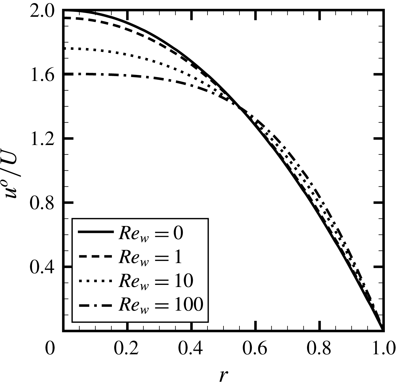
only. Figure 3 presents the profiles for
 $u^{o}/U$
for several wall Reynolds numbers. A small change occurs in the profiles, with the non-dimensional centreline velocity varying from approximately 1.6 for a wall with large injection to 2.0 for no injection of mass. For the case of a wall with no injection, the Poiseuille parabolic profile is obtained. These results agree with the ones reported in the literature (Eckert et al.
Reference Eckert, Donoughe and Moore1957; Berman Reference Berman1958; White Reference White1962; Kinney Reference Kinney1968; Terrill & Thomas Reference Terrill and Thomas1969; Raithby Reference Raithby1971).
Fully developed velocity profiles for wall Reynolds numbers 0, 1, 10 and 100.

It is worth noting that, as in Prandtl’s boundary layer theory, the similarity variable
 $F$
is a function of the radial coordinate stretched in the longitudinal direction. For that reason, the boundary condition at the tube inlet for different values of
 $Re_{w}$
is not equivalent to the Poiseuille parabolic profile, but of a Berman (Reference Berman1953) flow type (Haldenwang Reference Haldenwang2007). Consequently, close to the inlet, the velocity field obtained through (2.24b
) is not expected to match experimental measurements in which the flow is allowed to attain a Poiseuille velocity profile before entering the porous walled tube, but in the downstream region it would asymptotically approach the observations (Raithby & Knudsen Reference Raithby and Knudsen1974).
The wall Reynolds number is defined in terms of the dimensional wall injection velocity
 $\hat{V}_{w}$
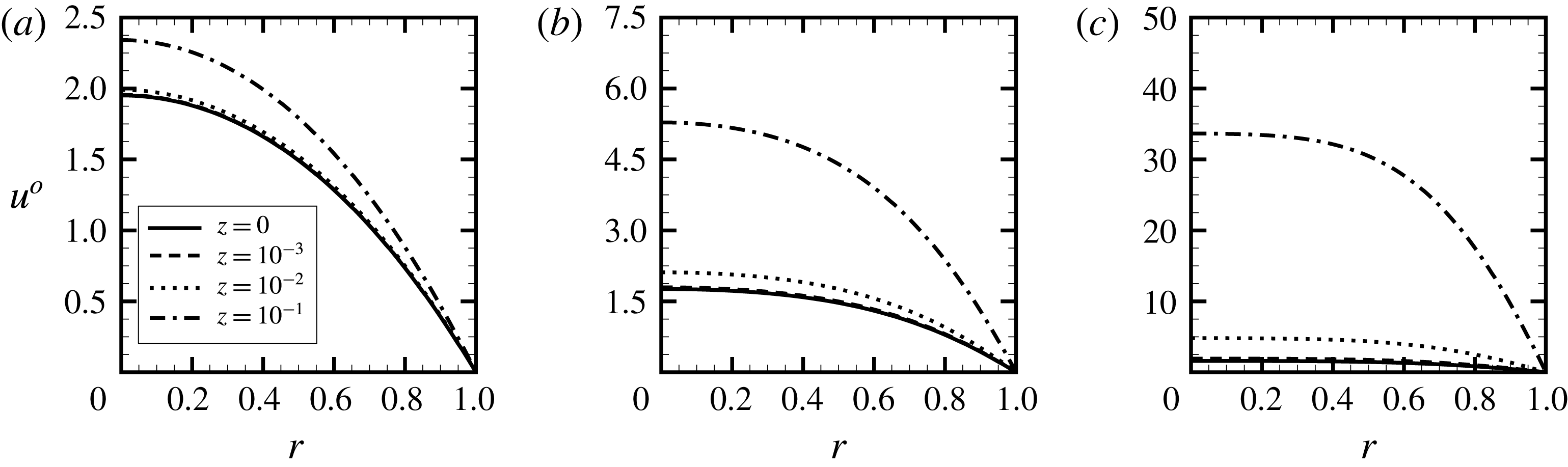
. Equivalently, it can also be described by the axial Reynolds number, as shown in (2.22). Therefore, the wall Reynolds number provides complete characterization of the dimensionless velocity field of a fluid in a tube with mass injection at the walls. The radial distribution of the axial velocity profiles for different axial positions
 $z$
is shown in figure 4, where the effect of increasing
 $Re_{w}$
is observed.
Axial velocity component profile at different
 $z$
for selected wall Reynolds numbers: (a)
 $Re_{w}=1$
, (b)
 $Re_{w}=10$
, (c)
 $Re_{w}=100$
.

Tangential velocity component profile at different
 $z$
for selected wall Reynolds numbers: (a)
 $Re_{w}=0$
, (b)
 $Re_{w}=1$
, (c)
 $Re_{w}=10$
.

3.2 Swirl velocity
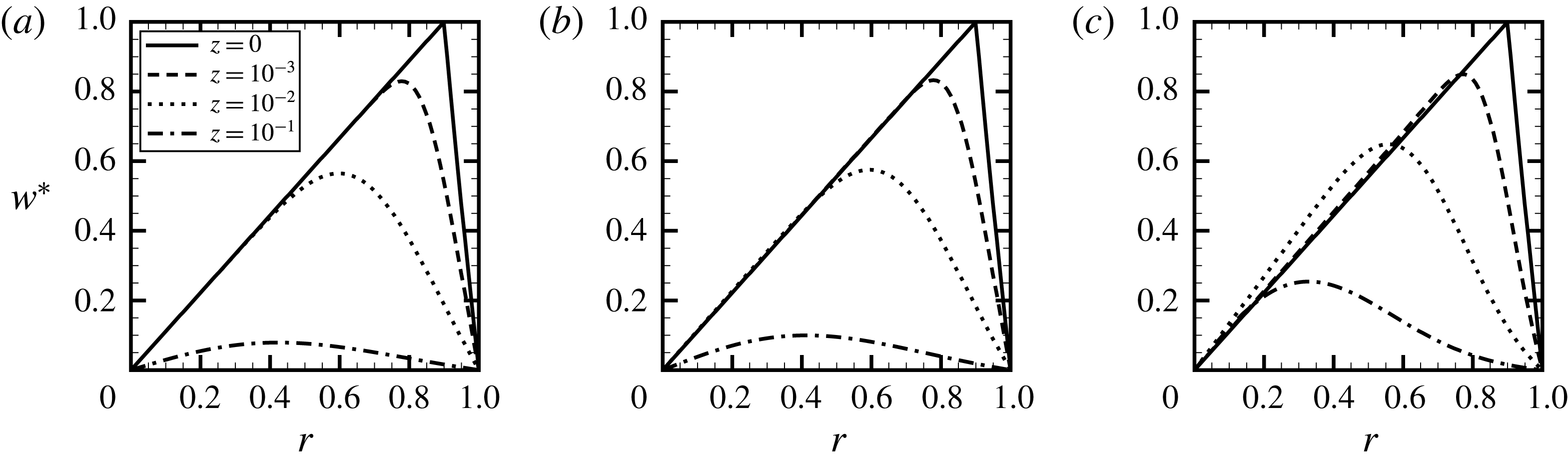
The decay of the inlet distribution of the swirl velocity component for different axial positions
 $z$
is shown in figure 5, where the effect of increasing
 $Re_{w}$
is observed. It is assumed that the position where the transition from forced to free vortex occurs is
 $r_{o}=0.9$
. The plots show the influence of the swirl velocity on the fluid flow without (figure 5
a) and with (figure 5
b,c) injection of mass through the wall. It is observed that the decay of the swirl velocity with
 $z$
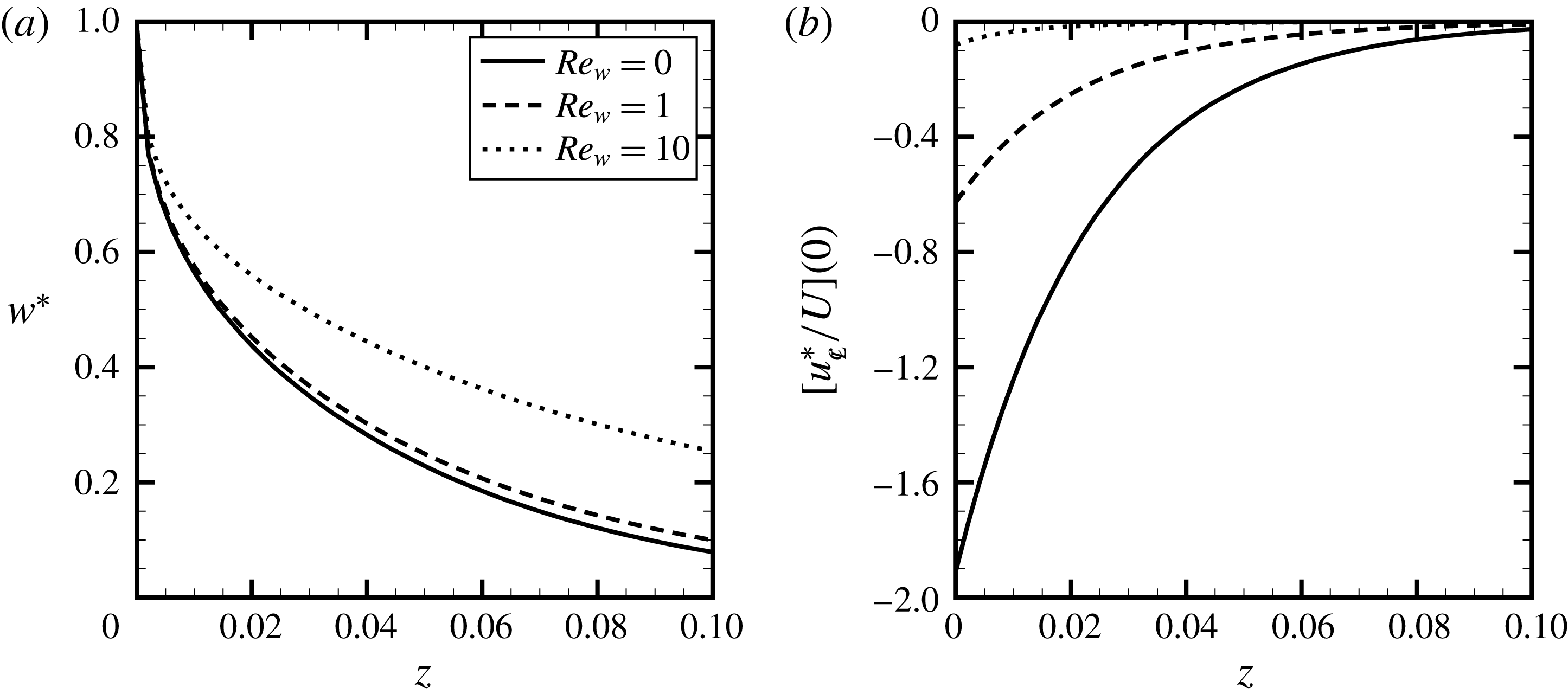
decreases with increasing values of the wall injection Reynolds number. This effect is shown more clearly in figure 7(a) where the maximum value of the swirl velocity is plotted as a function of the scaled axial coordinate
 $z$
for the same values of wall injection Reynolds numbers. As observed by Kinney & Sparrow (Reference Kinney and Sparrow1970), the decay of swirl velocity has a boundary layer character that confines the retarding action of the tube wall to the inner region (a layer adjacent to the wall surface) and the initial swirl distribution to the outer region. Figure 5 shows that the thickness of the inner layer is a function of the wall injection Reynolds number
 $Re_{w}$
.
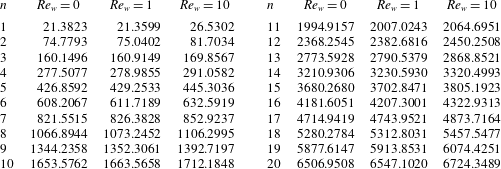
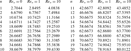
Modes
 $K_{n}$
as functions of
 $\hat{z}$
for selected wall Reynolds numbers: (a)
 $Re_{w}=0$
, (b)
 $Re_{w}=1$
, (c)
 $Re_{w}=10$
.

Peak values of the velocity components as a function of
 $z$
for selected wall Reynolds numbers. (a) Swirl velocity, (b) axial perturbation velocity.

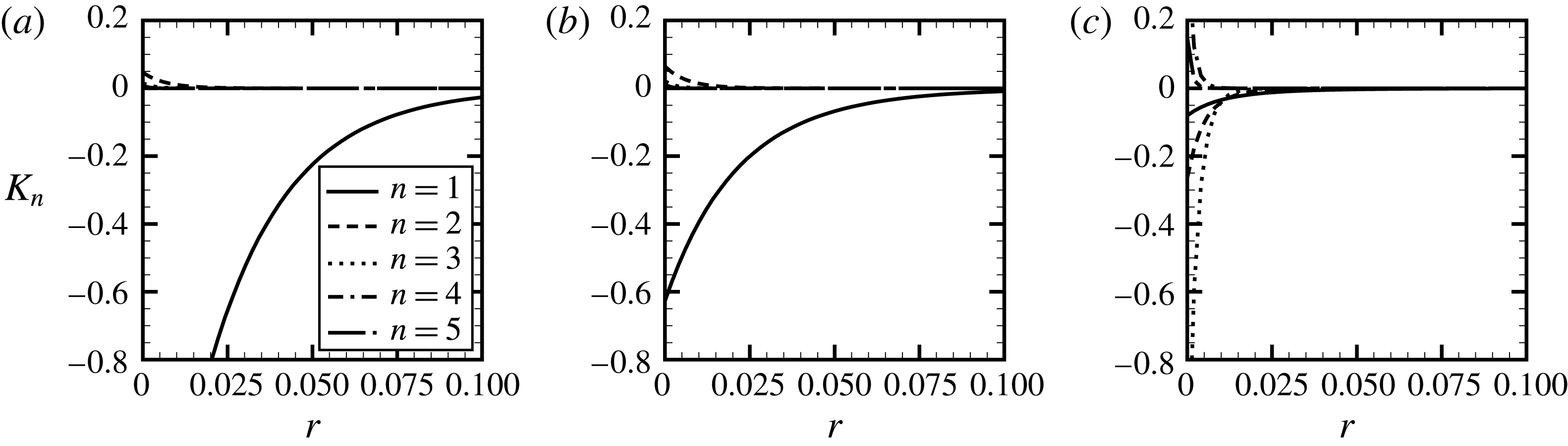
Following previous analyses in which the axial and radial perturbations induced by the swirl velocity were calculated, only the first term in the series in (2.42) is taken into account (Talbot Reference Talbot1954; Kinney & Sparrow Reference Kinney and Sparrow1970). The first term in the series is dominant at axial locations
 $z>10^{-2}$
. If all terms in the expansion were included, the decay of the perturbation induced by the swirl to the axial velocity would not be monotonic for all
 $Re_{w}$
, which is consistent mathematically but not physically. Each mode
 $K_{n}$
in the sum in (2.43), where
 $$\begin{eqnarray}K_{n}\equiv \frac{B_{n}U^{-(1+\unicode[STIX]{x1D706}_{n}/Re_{w})}}{C_{2}-2C_{1}(Re_{w}+\unicode[STIX]{x1D706}_{n})},\end{eqnarray}$$
has a varying influence on the total because of their different dependency on
 $Re_{w}$
. Hence, from (2.43), each mode decays monotonically, as observed in figure 6 for
 $n$
from 1 to 5, but their sum need not behave the same way. Therefore, the decay of each term represents correctly the influence of the swirl perturbation on other velocity components, but the sum does not. This behaviour is mainly due to the lack of higher-order terms that would include corrections for the diffusion of the induced perturbation.
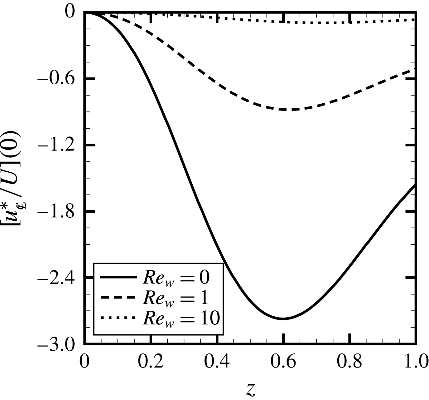
The perturbation due to the swirl influences the axial and radial velocity components. Therefore, as the initial swirl decays so does the effect it induces in the other velocity components. The maximum swirl intensity and the perturbation induced by the swirling flow in the axial velocity at the centreline are shown in figure 7 for selected
 $Re_{w}$
as a function of the scaled axial coordinate
 $z$
. The results from figure 7(b) should be treated with care. It is important to point out that the axial and radial perturbations due to the swirl are
 $O(\unicode[STIX]{x1D700}^{2})$
effects and that mass injection through the walls creates an increase in the mean axial velocity several orders of magnitude greater than the swirl-induced perturbation.
The effect of the inlet swirl intensity can also be evaluated. It is observed from figure 7(b) that the axial perturbation is strongly influenced by the magnitude of the injection of mass through the tube walls. Therefore, as
 $Re_{w}$
increases, larger values for
 $W_{0}$
are needed for the radial and axial velocity components to be affected by the perturbations due to the swirl. At the same time, equation (2.44) imposes a limiting restriction to the model at the inlet. In the vicinity of that region, the swirl intensity is maximum, and the magnitude of the induced perturbation is limited by its order. From figure 7(b), it is observed that (2.44) is indeed satisfied, i.e.
 . The maximum intensity
 $W_{0}$
is assumed to be around 0.5, which corresponds to an inlet flow swirl angle
 $\unicode[STIX]{x1D703}$
of approximately
 $27^{\circ }$
. (This value for the maximum swirl intensity minimally satisfies the constraints imposed by the perturbation orders.) As observed from figure 7(b), the chosen
 $W_{0}$
induces axial perturbations of absolute values as large as 0.48, 0.16 and 0.02 for
 $Re_{w}=0$
, 1 and 10, respectively.
A prescribed inlet swirl velocity distribution
 $w_{0}^{\ast }$
, given in (2.31), is considered. For such velocity distribution, the maximum intensity of the swirl is not solely responsible for the perturbation, even though it defines its order. The term
 $B_{n}$
, defined in (2.41a
), which can be seen as a projection of the function
 $w_{0}^{\ast }$
, represents the normalized inlet swirl radial profile squared. Therefore, the magnitude of the perturbation is also influenced by the radial distribution of
 $w_{0}^{\ast }$
. The effect of different values of
 $r_{0}$
on
 at
 $z=0$
is presented in figure 8. For
 $r_{0}$
greater than 0.7, which would correspond to commonly observed conditions, the influence of the position where the swirl velocity transitions from forced to free vortex is reduced. At the same time, the larger the injection, the smaller will be the effect of the inlet swirl distribution on the axial induced perturbation. The results in figure 8 also show that a larger perturbation is created for
 $r_{0}\simeq 0.6$
. This parameter could be considered in the design of swirl vanes that are intended to induce stronger perturbations.
Maximum intensity of the axial perturbation induced by the swirl flow at the inlet versus
 $r_{o}$
for wall Reynolds numbers 0, 1, 10.

Variation of
 $\unicode[STIX]{x1D6E9}$
with
 $z$
at selected radial positions for wall Reynolds 1 and 10.

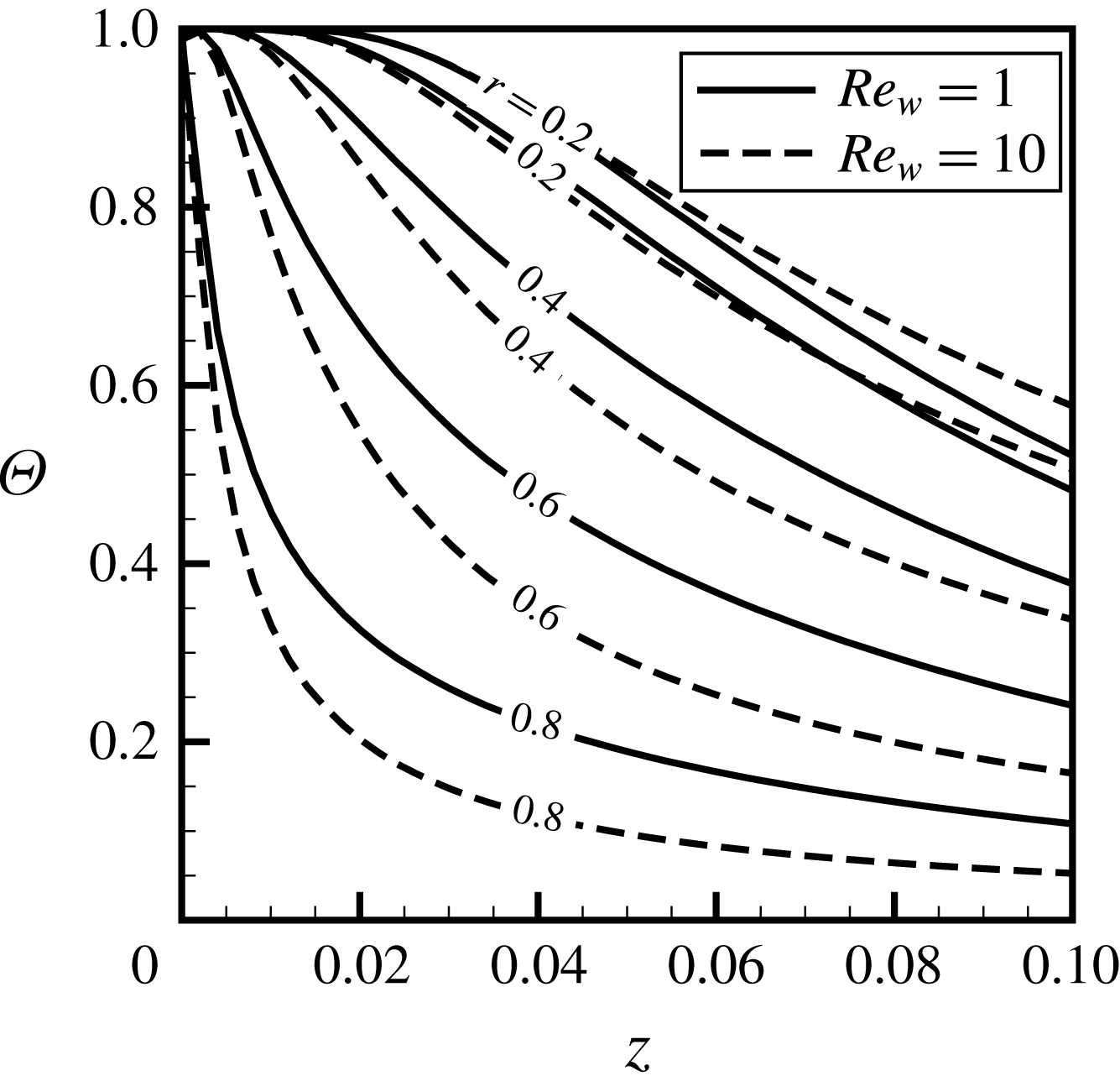
3.3 Perturbed scalar field
Before proceeding to the analysis of the tubular flame system, the solution for the scalar field is presented. Since it is assumed that the boundary condition at the wall is of the first type, i.e. a prescribed value for the conserved scalar, the solution for both the mixture fraction
 $Z$
and excess enthalpy
 $H$
can be scaled in terms of the function
 $\unicode[STIX]{x1D6E9}$
, defined in (2.51). The solution for the perturbed fields for wall Reynolds numbers 1 and 10, for selected radial positions, as a function of the scaled axial coordinate
 $z$
is presented in figure 9. The solution for the case of impermeable walls (
 $Re_{w}=0$
) is not shown in figure 9 because in the present model fuel evaporates from the wall, which corresponds to
 $Re_{w}$
greater than zero.
The effect of the perturbations induced by the swirl velocity on the scalar field are prominent in the inner region, i.e. in the zone close to the wall surface, and it is solely due to the terms on the right-hand side of (2.53). That occurs because the swirl improves mixing in the inner region, while in the outer region, where a free vortex-like structure exists, mixing is not favoured. As a consequence, in the inner zone, the transport from the walls is increased in comparison to the undisturbed case.
4 Results
The theoretical model is employed in the analysis of the structure of non-premixed swirl-type tubular flames. The generality of the formulation allows it to be applied to various conditions. However, we limit the results to conditions in which experimental studies would be of interest.
The flows considered in this analysis are laminar, such that their Reynolds numbers are of the order of hundreds, or a few thousands. Consequently, the range of values for the scaled axial coordinate
 $z$
we are interested in does not span up to higher values. Results are discussed considering
 $Re_{0}=500$
and the burner axial length
 $z_{max}=0.02$
. This choice does not limit the application of the theoretical model, but allows a physical interpretation that matches existing small-scale tubular flame systems, in which the length of the burner is commonly not greater than ten times its inner radius. The evaluation of the solution for a smaller portion of the domain also allows the analysis to be focused on the region where the influence of the swirling flow is more prominent, as observed in figure 7. It also means that, at the exit port of the burner, a swirling flow would still be found.
The intensity of Stefan convection, i.e. the vaporization rate of the fuel from the porous walls, determines the range of
 $Re_{w}$
, which can be estimated roughly from an overall mass conservation at the flame, assuming stoichiometric burning. If all the entraining air and injected fuel up to the axial location
 $z_{max}$
were completely consumed at the flame sheet, the mass flow rates of air and fuel necessary for the stoichiometric burning would be
 $$\begin{eqnarray}2SRe_{w}z_{max}=1,\end{eqnarray}$$
which can be employed to determine the values of
 $V_{w}$
used as starting estimate for the Stefan convection velocity. It is worth noting that (4.1) shows that for a fuel burning stoichiometrically, longer tubes would require lower wall injection Reynolds numbers. Assuming the maximum length of the tube as
 $z_{max}$
, the choice of fuel will influence the conserved scalar field through
 $Re_{w}$
, via its latent heat of vaporization
 $L$
, and the amount of heat release from the chemical reaction though
 $\unicode[STIX]{x1D6FE}$
. These parameters do not vary significantly for hydrocarbons, such as some higher carbon alkanes, which are found in condensed phase in standard conditions, and commonly employed in the evaluation of combustion systems. From (4.1), for stoichiometric conditions, the values of
 $Re_{w}$
for hexane, heptane and octane are, approximately, 1.7. At the same time, for those hydrocarbons, experimental peak flame temperatures are
 $T_{f}\simeq 4.5$
, which corresponds to
 $\unicode[STIX]{x1D6FE}\simeq 4.5$
. For that reason we will consider a single condition, which represented a number of alkanes found in liquid phase at ambient temperature and pressure.
In order to determine
 $V_{w}$
the procedure described in § 2 is employed. An initial guess is considered to calculate the excess-enthalpy field, and (2.18b
) is used to correct
 $V_{w}$
until its value is equal to the average of
 $|v_{w^{-}}|$
over the length of interest. The axial distance
 $z$
over which the mean value is obtained spans the final 80 % of the tube. The approximation of
 $|v_{w^{-}}|$
by a constant value
 $V_{w}$
corresponds to its zeroth order, and can be relaxed by employing a formulation in which a non-uniform
 $Re_{w}$
is assumed, for example, by considering a local pressure-dependent injection (Galowin, Fletcher & Desantis Reference Galowin, Fletcher and Desantis1974; Haldenwang Reference Haldenwang2007). With the correct approximation for
 $Re_{w}$
, the perturbed vector and scalar fields can be sought.
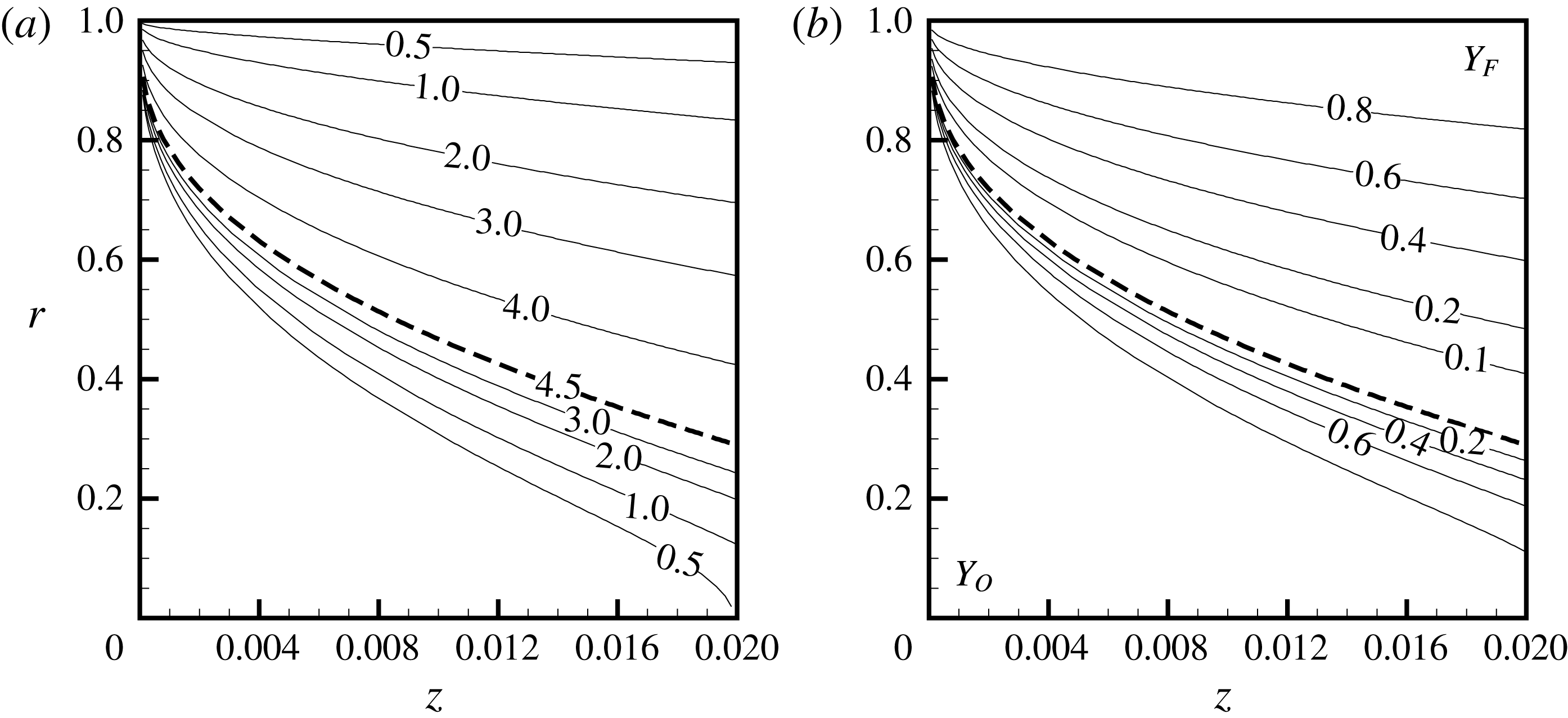
Contours of dimensionless scalar fields. The dashed line represents the flame sheet. (a) Temperature, (b) mass fraction.

Contours of the non-dimensional temperature field and mass fractions are presented in figures 10(a) and 10(b), respectively. The flame position, obtained as the location where the mixture fraction satisfies (2.15), is highlighted. The contour levels represent the non-dimensional temperature. The fuel side and the oxidizer side are indicated in figure 10(b) by
 $Y_{\text{F}}$
and
 $Y_{\text{O}}$
, respectively, where the levels represent the non-dimensional mass fractions on each side. It is observed that, even though the flame gets closer to the axis of the tube in the downstream region, the tube is not long enough for the flame sheet to close before reaching the tube outlet. The calculated wall injection Reynolds number is approximately
 $9$
. That corresponds to a fuel-rich condition, considering the stoichiometric value 1.7 obtained from relation (4.1). Even though the stoichiometric and the calculated
 $Re_{w}$
are of the same order of magnitude, it is important to point out that the solution does not incorporate other thermal losses that could be added to the effective latent heat of vaporization to reduce the estimated fuel injected using (2.18b
). At the same time, effects such as finite rate chemistry, variations of transport and thermodynamic properties with temperature or concentration, radiation losses, non-equilibrium temperature effects between the porous matrix and the liquid phase, radial or axial temperature variations in the wall, axial heat transfer in the porous matrix, spatial variation of the vaporization rate, among several others, are not considered in the solution. Therefore, given the approximations involved, the analytical result is expected to predict only qualitatively flame characteristics, similarly to the solution obtained by the Burke–Schumann model for coflow flames. Indeed, the non-premixed flame established in this configuration resembles the latter solution for the so-called underventilated case. In this condition, the flame is established above a coflow burner from which the amount of air issued is smaller than that necessary to burn all the injected fuel, and the flame extends into the oxidizer region. The non-dimensional temperature and species contours in figure 10 possess the same characteristics.
The fuel-rich inlet conditions and the results from figure 10(b) indicate that a mixture of unburned fuel and products is found at the burner outlet. This condition resembles the experimental observations for the miniature liquid film burner (Pham et al.
Reference Pham, Dunn-Rankin and Sirignano2007). Results in the downstream region of the combustion chamber, i.e. after the exit port, cannot be predicted by the model, but the characteristic of the external flame can be qualitatively estimated. As a consequence of the absence of tube walls that constrain the flow and act as a fuel source to the chemical reaction at axial positions greater than the burner length
 $z_{max}$
, the flame would expand outwards in the radial direction due to the centrifugal force, and its shape would no longer possess a tubular structure, but a conical structure instead. The external flame shape would also be due to the excess air found in the environment reacting with the mixture of hot unburned fuel and products if the burner is exposed to normal ambient conditions.
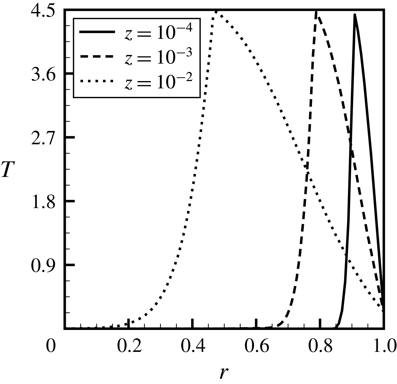
Variation of non-dimensional temperature with
 $r$
at selected axial positions.

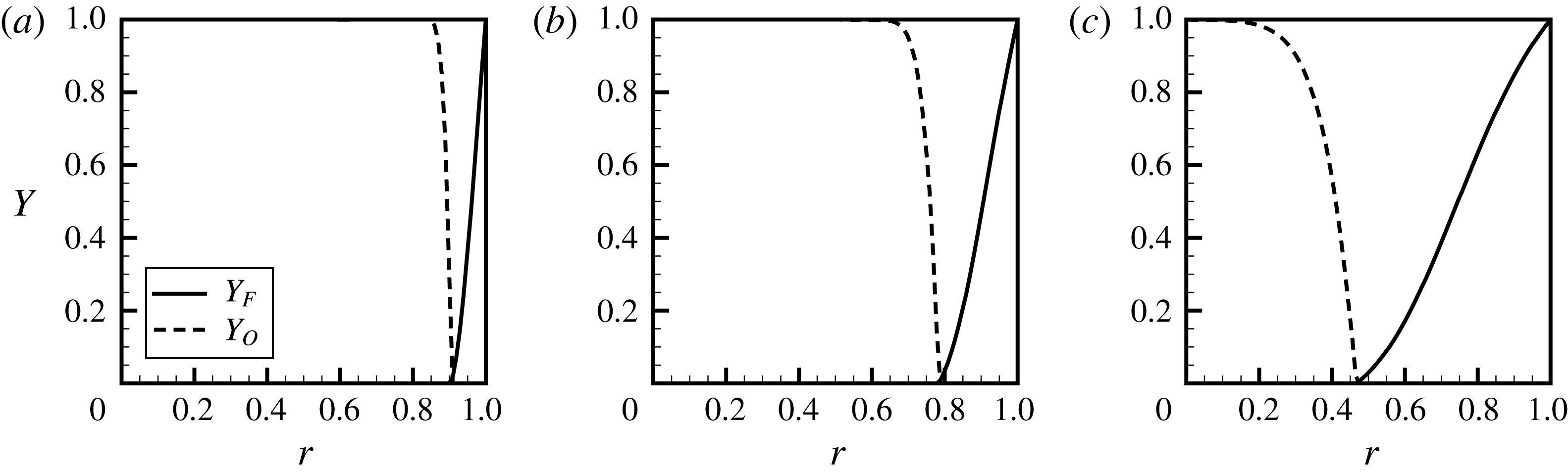
Dimensionless temperature and mixture fraction profiles are shown, respectively, in figures 11 and 12 for selected axial positions as a function of the radial coordinate
 $r$
. The variation of temperature and mixture fraction along the radial direction resembles the profiles obtained in non-premixed counterflow configurations for axial locations near the inlet as expected for a non-premixed system. The flame is located, for each of the axial positions
 $z$
as the temperature peak, in figure 11, and as the minima, in figure 12. The effect of the flame sheet extending into the oxidizer region for larger axial locations is clearly observed.
Variation of non-dimensional mixture fraction profiles at selected axial positions: (a)
 $z=10^{-4}$
, (b)
 $z=10^{-3}$
, (c)
 $z=10^{-2}$
.

5 Conclusions
A theoretical model for non-premixed swirl-type tubular flames burning condensed fuels with unity Lewis numbers is presented. The formulation allows the determination of the velocity, temperature and species fields. Results are discussed considering a similarity solution for axisymmetric incompressible viscous flow fields. Axial decay of the initial swirl velocity, its induced axial and radial perturbations to the flow, temperature and species field together with surface mass and heat transfer from the porous walls are considered through the superposition of laminar swirling flow on a Berman flow with uniform mass injection in a straight pipe. The flame structure is obtained assuming infinitely fast conversion of reactants into products and unity Lewis numbers, allowing the application of Shvab–Zel’dovich variables.
Results from the perturbation analysis consider constant temperature at the walls, more specifically, at the fuel boiling point. Non-dimensional temperature and species profiles are presented for conditions in which experimental results would be of interest. The balance between the amount of energy necessary for the fuel to be heated from the injection temperature to its boiling point and the energy released by the reaction show that the system operates in fuel-rich conditions. The flame extends towards the oxidizer region as it is observed in the underventilated case for the Burke–Schumann model.
The theoretical model can provide qualitative guidelines to the design of non-premixed swirl-type tubular systems, such as the influence of inlet or dimensional parameters on flame position, flame confinement as well as overall system temperature and heat transfer. The analytical expressions presented herein, which are developed in a simplified framework, allow a fast and comprehensive description of the temperature, species and flow fields for the system.
Appendix A. Details of the derivations
A.1 Swirl decay of axial velocity
Both sides of (2.28) are functions of only one independent variable, thus its solution can be found by a separation of variables in the form
 $$\begin{eqnarray}w^{\ast }(r,z)=\unicode[STIX]{x1D719}(r)\unicode[STIX]{x1D713}(z),\end{eqnarray}$$
which can be substituted into (2.28), yielding
 $$\begin{eqnarray}\frac{2}{F\unicode[STIX]{x1D719}}\left[\frac{\text{d}^{2}\unicode[STIX]{x1D719}}{\text{d}r^{2}}+\left(\frac{Re_{w}G}{2}+\frac{1}{r}\right)\frac{\text{d}\unicode[STIX]{x1D719}}{\text{d}r}+\left(\frac{Re_{w}G}{2}-\frac{1}{r}\right)\frac{\unicode[STIX]{x1D719}}{r}\right]=\frac{1+2Re_{w}z}{\unicode[STIX]{x1D713}}\frac{\text{d}\unicode[STIX]{x1D713}}{\text{d}z}=-\unicode[STIX]{x1D706}.\end{eqnarray}$$
The solution for the axial direction is obtained by integrating the equation for
 $\unicode[STIX]{x1D713}(z)$
as
 $$\begin{eqnarray}\unicode[STIX]{x1D713}(z)=c(1+2Re_{w}z)^{-\unicode[STIX]{x1D706}/(2Re_{w})},\end{eqnarray}$$
where
 $c$
is the constant of integration. The equation for
 $\unicode[STIX]{x1D719}(r)$
is given by
 $$\begin{eqnarray}\frac{\text{d}^{2}\unicode[STIX]{x1D719}}{\text{d}r^{2}}+\left(\frac{Re_{w}G}{2}+\frac{1}{r}\right)\frac{\text{d}\unicode[STIX]{x1D719}}{\text{d}r}+\left(\frac{Re_{w}G}{2}-\frac{1}{r}\right)\frac{\unicode[STIX]{x1D719}}{r}+\unicode[STIX]{x1D706}\frac{F}{2}\unicode[STIX]{x1D719}=0,\end{eqnarray}$$
which can be cast into Sturm–Liouville form through the introduction of an integrating factor,
 $$\begin{eqnarray}q_{\unicode[STIX]{x1D719}}(r)=\exp \int \left(\frac{Re_{w}G}{2}+\frac{1}{r}\right)\,\text{d}r,\end{eqnarray}$$
yielding
 $$\begin{eqnarray}\frac{\text{d}}{\text{d}r}\left(q_{\unicode[STIX]{x1D719}}\frac{\text{d}\unicode[STIX]{x1D719}}{\text{d}r}\right)+\left[\frac{q_{\unicode[STIX]{x1D719}}}{r}\left(\frac{Re_{w}G}{2}-\frac{1}{r}\right)\right]\unicode[STIX]{x1D719}+\unicode[STIX]{x1D706}\unicode[STIX]{x1D70E}_{\unicode[STIX]{x1D719}}\unicode[STIX]{x1D719}=0,\end{eqnarray}$$
where the weight function
 $\unicode[STIX]{x1D70E}_{\unicode[STIX]{x1D719}}(r)$
is given by
 $$\begin{eqnarray}\unicode[STIX]{x1D70E}_{\unicode[STIX]{x1D719}}(r)=q_{\unicode[STIX]{x1D719}}F/2.\end{eqnarray}$$
The swirl velocity
 $w^{\ast }$
must vanish at the tube wall (
 $r=1$
) and at the axis of symmetry (
 $r=0$
). These conditions must be satisfied for all
 $z$
, such that
 $\unicode[STIX]{x1D719}(0)=\unicode[STIX]{x1D719}(1)=0$
. The solution of (A 6) for all eigenfunctions is obtained numerically using a collocation method (Kierzenka & Shampine Reference Kierzenka and Shampine2001). An initial guess and a condition for the eigenvalues
 $\unicode[STIX]{x1D706}$
are necessary to solve (A 6) numerically. The orthogonality condition, which requires that, for orthonormal eigenfunctions,
 $$\begin{eqnarray}\int _{0}^{1}\unicode[STIX]{x1D719}_{m}(r)\unicode[STIX]{x1D719}_{n}(r)\unicode[STIX]{x1D70E}_{\unicode[STIX]{x1D719}}(r)\,\text{d}r=\unicode[STIX]{x1D6FF}_{mn}\Vert \unicode[STIX]{x1D719}_{n}\Vert ^{2}\end{eqnarray}$$
is solved together with (A 6) to determine each eigenfunction–eigenvalue pair – a classical approach for the numerical solution of Sturm–Liouville problems (Ascher Reference Ascher1980). The solution for the special case
 $Re_{w}=0$
is used as the starting estimate to the one for any
 $Re_{w}$
since the solution for the problem with surface mass transfer at the walls presents a relatively small deviation from the special case of impermeable walls. The solution for
 $Re_{w}=0$
is given in terms of the confluent hypergeometric function of the first kind
 $\text{}_{1}F_{1}$
(Abramowitz & Stegun Reference Abramowitz and Stegun1965) as (Talbot Reference Talbot1954)
 $$\begin{eqnarray}\unicode[STIX]{x1D719}_{n}^{0}(r)=\unicode[STIX]{x1D706}_{n}^{1/4}r\exp \left(-\frac{\sqrt{\unicode[STIX]{x1D706}_{n}}}{2}r^{2}\right)\text{}_{1}F_{1}\left(1-\frac{\sqrt{\unicode[STIX]{x1D706}_{n}}}{4},2,\sqrt{\unicode[STIX]{x1D706}_{n}}r^{2}\right).\end{eqnarray}$$
Denoting the
 $n$
th eigenfunction of (A 6) as
 $\unicode[STIX]{x1D719}_{n}(r)$
, the swirl velocity
 $w^{\ast }(z,r)$
for any
 $Re_{w}$
can be expressed as
 $$\begin{eqnarray}w^{\ast }(r,z)=\mathop{\sum }_{n=1}^{\infty }c_{n}\unicode[STIX]{x1D719}_{n}(r)(1+2Re_{w}z)^{-\unicode[STIX]{x1D706}_{n}/(2Re_{w})}.\end{eqnarray}$$
For the special case of tubes with impermeable walls, the swirl velocity is given by
 $$\begin{eqnarray}w^{\ast }(r,z)=\mathop{\sum }_{n=1}^{\infty }c_{n}\unicode[STIX]{x1D719}_{n}^{0}(r)\exp (-\unicode[STIX]{x1D706}_{n}z).\end{eqnarray}$$
A total of sixty terms are considered in the sum in (A 10). The first twenty eigenvalues for selected
 $Re_{w}$
are given in table 1.
First twenty eigenvalues
 $\unicode[STIX]{x1D706}_{n}$
for selected
 $Re_{w}$
.

A.2 Axial and radial perturbations velocities
In order to determine the perturbation velocities
 $u^{\ast }$
and
 $v^{\ast }$
, we eliminate the pressure gradients by differentiating equation (2.2) with respect to
 $r$
and (2.3) with respect to
 $z$
, and subtracting one from the other (Kinney & Sparrow Reference Kinney and Sparrow1970). A single equation can be written in terms of the tangential component of vorticity
 $\unicode[STIX]{x1D714}$
. We neglect the streamwise diffusion terms,
 $$\begin{eqnarray}\frac{u}{Re_{0}}\frac{\unicode[STIX]{x2202}\unicode[STIX]{x1D714}}{\unicode[STIX]{x2202}z}+v\frac{\unicode[STIX]{x2202}\unicode[STIX]{x1D714}}{\unicode[STIX]{x2202}r}-\frac{v\unicode[STIX]{x1D714}}{r}-\frac{1}{Re_{0}}\frac{\unicode[STIX]{x2202}}{\unicode[STIX]{x2202}z}\left(\frac{w^{\ast 2}}{r}\right)=\frac{2}{Re_{0}}\left(\frac{\unicode[STIX]{x2202}^{2}\unicode[STIX]{x1D714}}{\unicode[STIX]{x2202}r^{2}}+\frac{1}{r}\frac{\unicode[STIX]{x2202}\unicode[STIX]{x1D714}}{\unicode[STIX]{x2202}r}-\frac{\unicode[STIX]{x1D714}}{r^{2}}\right),\end{eqnarray}$$
and denote
 $$\begin{eqnarray}\unicode[STIX]{x1D714}=\unicode[STIX]{x1D714}^{o}+\unicode[STIX]{x1D714}^{\ast }.\end{eqnarray}$$
We then substitute (A 13) together with (2.19) into (A 12), and retain first-order terms only, that is,
 $$\begin{eqnarray}\displaystyle & & \displaystyle \frac{u^{\ast }}{Re_{0}}\frac{\unicode[STIX]{x2202}\unicode[STIX]{x1D714}^{o}}{\unicode[STIX]{x2202}z}+\frac{u^{o}}{Re_{0}}\frac{\unicode[STIX]{x2202}\unicode[STIX]{x1D714}^{\ast }}{\unicode[STIX]{x2202}z}+v^{\ast }\frac{\unicode[STIX]{x2202}\unicode[STIX]{x1D714}^{o}}{\unicode[STIX]{x2202}r}+v^{o}\frac{\unicode[STIX]{x2202}\unicode[STIX]{x1D714}^{\ast }}{\unicode[STIX]{x2202}r}-\frac{v^{\ast }\unicode[STIX]{x1D714}^{o}}{r}-\frac{v^{o}\unicode[STIX]{x1D714}^{\ast }}{r}-\frac{1}{Re_{0}}\frac{\unicode[STIX]{x2202}}{\unicode[STIX]{x2202}z}\left(\frac{w^{\ast 2}}{r}\right)\qquad \nonumber\\ \displaystyle & & \displaystyle \quad =\frac{1}{Re_{0}}\left(\frac{\unicode[STIX]{x2202}^{2}\unicode[STIX]{x1D714}^{\ast }}{\unicode[STIX]{x2202}r^{2}}+\frac{1}{r}\frac{\unicode[STIX]{x2202}\unicode[STIX]{x1D714}^{\ast }}{\unicode[STIX]{x2202}r}-\frac{\unicode[STIX]{x1D714}^{\ast }}{r^{2}}\right),\end{eqnarray}$$
which can be further simplified if we note that
 $$\begin{eqnarray}\unicode[STIX]{x1D714}^{o}=-\frac{\unicode[STIX]{x2202}u^{o}}{\unicode[STIX]{x2202}r}\quad \text{and}\quad \unicode[STIX]{x1D714}^{\ast }=-\frac{\unicode[STIX]{x2202}u^{\ast }}{\unicode[STIX]{x2202}r}.\end{eqnarray}$$
Substituting the expressions for
 $\unicode[STIX]{x1D714}^{o}$
,
 $\unicode[STIX]{x1D714}^{\ast }$
,
 $u^{o}$
and
 $v^{o}$
into (A 14), we obtain the expression shown in (2.32). To solve the system composed of (2.32) and (2.33), we assume (Kinney & Sparrow Reference Kinney and Sparrow1970)
 $$\begin{eqnarray}u^{\ast }=\mathop{\sum }_{n=0}^{5}a_{n}(z)r^{n}.\end{eqnarray}$$
The choice of approximating the solution by a polynomial is made for simplicity, and its suitability has been discussed by several authors (Talbot Reference Talbot1954; Kinney & Sparrow Reference Kinney and Sparrow1970; Verma & Gaur Reference Verma and Gaur1974). The solution can also be obtained by other techniques, such as the Green’s function method (Deka Reference Deka1963, Reference Deka1966) or integral transform (Lavan et al. Reference Lavan, Nielsen and Fejer1969). Therefore, the quintic function considered can be viewed as an approximation to the exact solutions.
In addition to the two boundary conditions on
 $u^{\ast }$
with respect to
 $r$
, one more can be obtained upon integrating (2.33):
 $$\begin{eqnarray}\int _{0}^{1}u^{\ast }r\,\text{d}r=0.\end{eqnarray}$$
Furthermore, the polynomial
 $u^{\ast }$
is required to satisfy (2.32) at the wall and at the symmetry axis (Kinney & Sparrow Reference Kinney and Sparrow1970):
 $$\begin{eqnarray}\displaystyle & \displaystyle \left[\frac{\unicode[STIX]{x2202}^{3}u^{\ast }}{\unicode[STIX]{x2202}r^{3}}+\left(\frac{\unicode[STIX]{x2202}^{2}u^{\ast }}{\unicode[STIX]{x2202}r^{2}}-\frac{\unicode[STIX]{x2202}u^{\ast }}{\unicode[STIX]{x2202}r}\right)\left(1+\frac{Re_{w}}{2}\right)\right]_{r=1}=0, & \displaystyle\end{eqnarray}$$
 $$\begin{eqnarray}\displaystyle & \displaystyle \left[\frac{\unicode[STIX]{x2202}^{3}u^{\ast }}{\unicode[STIX]{x2202}r^{3}}+\left(\frac{\unicode[STIX]{x2202}^{2}u^{\ast }}{\unicode[STIX]{x2202}r^{2}}-\frac{1}{r}\frac{\unicode[STIX]{x2202}u^{\ast }}{\unicode[STIX]{x2202}r}\right)\frac{1}{r}\right]_{r=0}=0. & \displaystyle\end{eqnarray}$$
 $a_{0}$
, given in (2.38).
The solution to ordinary differential equation for
 $a_{0}$
, equation (2.39), for the special case of tubes with impermeable walls is given by
 $$\begin{eqnarray}a_{0}^{0}=\mathop{\sum }_{n=1}^{\infty }\frac{B_{n}\exp (-2\unicode[STIX]{x1D706}_{n}z)}{C_{2}-2C_{1}\unicode[STIX]{x1D706}_{n}}.\end{eqnarray}$$
A.3 Undisturbed scalar field
Both sides of (2.47) are functions of only one independent variable. However, the boundary conditions for
 $H$
in the radial direction are not both homogeneous. We introduce the transformation
 $$\begin{eqnarray}\unicode[STIX]{x1D6E9}=-(H^{o}-H_{w})/H_{w},\end{eqnarray}$$
the conservation equation (2.46),
 $$\begin{eqnarray}\frac{2}{F}\left[\frac{\unicode[STIX]{x2202}^{2}\unicode[STIX]{x1D6E9}}{\unicode[STIX]{x2202}r^{2}}+\left(\frac{Pe_{w}}{2}G+\frac{1}{r}\right)\frac{\unicode[STIX]{x2202}\unicode[STIX]{x1D6E9}}{\unicode[STIX]{x2202}r}\right]=(1+2Re_{w}z)Pr\frac{\unicode[STIX]{x2202}\unicode[STIX]{x1D6E9}}{\unicode[STIX]{x2202}z},\end{eqnarray}$$
with boundary conditions
 $$\begin{eqnarray}\left.\frac{\unicode[STIX]{x2202}\unicode[STIX]{x1D6E9}}{\unicode[STIX]{x2202}r}\right|_{r=0}=\unicode[STIX]{x1D6E9}(1,z)=\unicode[STIX]{x1D6E9}(r,0)-1=0.\end{eqnarray}$$
The solution is obtained by the separating
 $\unicode[STIX]{x1D6E9}(r,z)$
as
 $$\begin{eqnarray}\unicode[STIX]{x1D6E9}(r,z)=R(r)X(z).\end{eqnarray}$$
Substituting (A 20) and (A 23) into (2.46),
 $$\begin{eqnarray}\frac{2}{FR}\left[\frac{\text{d}^{2}R}{\text{d}r^{2}}+\left(\frac{Pe_{w}}{2}G+\frac{1}{r}\right)\frac{\text{d}R}{\text{d}r}\right]=(1+2Re_{w}z)Pr\frac{1}{X}\frac{\text{d}X}{\text{d}z}=-\unicode[STIX]{x1D6FD}^{2},\end{eqnarray}$$
the solution for the axial direction is obtained by integrating the equation for
 $X(z)$
as
 $$\begin{eqnarray}X(z)=b(1+2Re_{w}z)^{-\unicode[STIX]{x1D6FD}^{2}/Pe_{w}},\end{eqnarray}$$
where
 $b$
is the constant of integration. The equation for
 $R(r)$
is given by
 $$\begin{eqnarray}\frac{\text{d}^{2}R}{\text{d}r^{2}}+\left(\frac{Pe_{w}}{2}G+\frac{1}{r}\right)\frac{\text{d}R}{\text{d}r}+\unicode[STIX]{x1D6FD}^{2}\frac{F}{2}R=0,\end{eqnarray}$$
which can be cast into Sturm–Liouville form through the introduction of an integrating factor,
 $$\begin{eqnarray}q_{R}(r)=\exp \int \left(\frac{Pe_{w}}{2}G+\frac{1}{r}\right)\,\text{d}r,\end{eqnarray}$$
yielding
 $$\begin{eqnarray}\frac{\text{d}}{\text{d}r}\left(q_{R}\frac{\text{d}R}{\text{d}r}\right)+\unicode[STIX]{x1D6FD}^{2}\unicode[STIX]{x1D70E}_{R}R=0,\end{eqnarray}$$
where the weight function
 $\unicode[STIX]{x1D70E}_{R}(r)$
is given by
 $$\begin{eqnarray}\unicode[STIX]{x1D70E}_{R}(r)=q_{R}F/2,\end{eqnarray}$$
such that the orthogonality property of the eigenfunctions
 $R_{n}(r)$
is given by
 $$\begin{eqnarray}\int _{0}^{1}R_{m}(r)R_{n}(r)\unicode[STIX]{x1D70E}_{R}(r)\,\text{d}r=\unicode[STIX]{x1D6FF}_{mn}\Vert R_{n}\Vert ^{2}.\end{eqnarray}$$
The solution
 $R_{n}^{0}(r)$
to the special case
 $Re_{w}=0$
,
 $$\begin{eqnarray}R_{n}^{0}(r)=\exp \left(-\frac{\unicode[STIX]{x1D6FD}_{n}}{2}r^{2}\right)\text{}_{1}F_{1}\left(\frac{1}{2}-\frac{\unicode[STIX]{x1D6FD}_{n}}{4},1,\unicode[STIX]{x1D6FD}_{n}r^{2}\right),\end{eqnarray}$$
can be used as the initial guess to the solution of (A 26). The methodology is the same as that used to obtain numerically the eigenfunction–eigenvalue pair for (A 26). Denoting the
 $n$
th eigenfunction of (A 26) as
 $R_{n}(r)$
, the dependent variable
 $\unicode[STIX]{x1D6E9}(z,r)$
for any
 $Re_{w}$
, is obtained as
 $$\begin{eqnarray}\unicode[STIX]{x1D6E9}(r,z)=\mathop{\sum }_{n=1}^{\infty }b_{n}R_{n}(r)(1+2Re_{w}z)^{-\unicode[STIX]{x1D6FD}_{n}^{2}/(2Pe_{w})}.\end{eqnarray}$$
For the special case of tubes with impermeable walls, the dependent variable
 $\unicode[STIX]{x1D6E9}(z,r)$
is given by
 $$\begin{eqnarray}\unicode[STIX]{x1D6E9}(z,r)=\mathop{\sum }_{n=1}^{\infty }b_{n}R_{n}^{0}(r)\exp (-\unicode[STIX]{x1D6FD}_{n}^{2}z/Pr).\end{eqnarray}$$
A total of sixty terms are considered in the sum in (A 32). The first twenty eigenvalues for selected
 $Re_{w}$
are given in table 2.
First twenty eigenvalues
 $\unicode[STIX]{x1D6FD}_{n}$
for selected
 $Re_{w}$
.