2 The asymptotic regimes of NIW modulation

Our goal in this section is to motivate the existence of different asymptotic regimes in which the modulation of the wave field by the mean flow can vary significantly. As mentioned, $Bu_{n}$ decreases from $O(1)$ for low modes to asymptotically small values for high modes, which means that wave energy and shear in real flows, which project onto a broad spectrum of modes, are distributed across interaction regimes ranging in dispersive strength. The cumulative effects of the background flow on NIWs depends on the distribution of $Bu_{n}$ with respect to the Rossby number.

Figure 1.

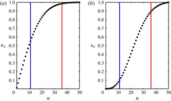
Fractional energy $e_{n}$ and fractional shear $s_{n}$ contained in the first 50 baroclinic modes. The blue and red curves correspond to $n_{0.125}\approx 11$ and $n_{0.0125}\approx 36$ , respectively, calculated based on (2.5). These curves demarcate between modes with stronger dispersion $Bu_{n}\gg \unicode[STIX]{x1D716}$ in (a) and weak dispersion modes with $Bu_{n}\leqslant \unicode[STIX]{x1D716}$ in (b). For example, if $\unicode[STIX]{x1D716}=0.0125$ (red line) then most of the wave energy and almost all of the wave shear is associated with strongly dispersive modes. Conversely, if $\unicode[STIX]{x1D716}=0.125$ (blue line) only about half of the energy and less than 10 % of the shear are associated with strongly dispersive modes. This illustrates the sensitivity of the relevant modal regimes to the Rossby number $\unicode[STIX]{x1D716}$ .

Consider a hypothetical storm-generated inertial wave horizontal velocity field, in complex form,

(2.1) $$\begin{eqnarray}\mathscr{U}=u+\text{i}v=A(z)\text{e}^{-\text{i}t},\quad \text{with}~A(z)=\exp \left(\frac{-z^{2}}{2h^{2}}\right),\end{eqnarray}$$

where $z=-h$ is the depth at which the inertial shear, $A^{\prime }(z)$ , is maximal and where $z=0$ is the surface. This is an exact solution to the linear equations without a balanced flow. Projecting (2.1) onto baroclinic modes one obtains (see appendix A for details)

(2.2a,b ) $$\begin{eqnarray}A(z)=\frac{A_{0}}{2}+\mathop{\sum }_{n=1}^{\infty }A_{n}\cos \left(\frac{n\unicode[STIX]{x03C0}z}{H}\right),\quad A_{n}=\frac{2}{H}\exp \left(-\frac{\unicode[STIX]{x03C0}^{2}n^{2}h^{2}}{2H^{2}}\right)\int _{-H}^{0}\exp \left(-\frac{z^{2}}{2h^{2}}\right)\,\text{d}z,\end{eqnarray}$$

and in the limit $h\ll H$ , the coefficients are approximately

(2.3) $$\begin{eqnarray}A_{n}\approx \frac{\sqrt{2\unicode[STIX]{x03C0}}h}{H}\exp \left(-\frac{\unicode[STIX]{x03C0}^{2}n^{2}h^{2}}{2H^{2}}\right).\end{eqnarray}$$

The fractions of total energy and total shear contained in the first $n$ baroclinic modes are

(2.4a,b ) $$\begin{eqnarray}e_{n}=\frac{\displaystyle \mathop{\sum }_{j=1}^{n}A_{j}^{2}}{\displaystyle \mathop{\sum }_{j=1}^{\infty }A_{j}^{2}}\quad \text{and}\quad s_{n}=\frac{\displaystyle \mathop{\sum }_{j=1}^{n}B_{j}^{2}}{\displaystyle \mathop{\sum }_{j=1}^{\infty }B_{j}^{2}},\end{eqnarray}$$

where $B_{j}=(j\unicode[STIX]{x03C0}/H)A_{j}$ corresponds to the Fourier coefficients of $A^{\prime }(z)$ . Figure 1 shows $e_{n}$ and $s_{n}$ , assuming an eddy length scale $L=40$  km, ocean depth $H=5$  km, buoyancy frequency $N=100f=10^{-2}~\text{s}^{-1}$ and shear depth $h=-75$  m. Motivated by the observations of wind-excited NIWs discussed in D’Asaro et al. (Reference D’Asaro, Eriksen, Levine, Niiler, Paulson and van Meurs1995), we also chose the balanced flow velocity $V_{g}=0.05~\text{m}~\text{s}^{-1}$ which gives $\unicode[STIX]{x1D716}=0.0125$ . For the numerical experiments that follow, we choose a second Rossby number, $\unicode[STIX]{x1D716}=0.125$ , an order of magnitude larger than the previous one. As mentioned before, the strength of modulation of the wave field by the mean flow is expected to depend on the fraction of modes with $Bu_{n}\sim \unicode[STIX]{x1D716}$ , where advection–refraction and dispersion coincide in strength. We construct a critical mode number for a given Rossby number as

(2.5) $$\begin{eqnarray}n_{\unicode[STIX]{x1D716}}=\frac{N_{0}H}{\unicode[STIX]{x03C0}fL\sqrt{\unicode[STIX]{x1D716}}}\end{eqnarray}$$

by equating modal Burger number (1.7) and Rossby number. The coloured vertical lines in figure 1 indicate $n_{0.125}$ and $n_{0.0125}$ . Notice that for the lower Rossby number case, fewer modes satisfy $Bu_{n}\lesssim \unicode[STIX]{x1D716}$ and therefore less energy is associated with the regime $Bu\sim \unicode[STIX]{x1D716}$ , as discussed before.

We now turn to some idealized simulations to validate our qualitative predictions. To illustrate that the modulation of the wave field depends strongly on the fraction of modes that satisfy $Bu_{n}\sim \unicode[STIX]{x1D716}$ versus those that satisfy $Bu_{n}\sim O(1)$ , we numerically integrate the linear Boussinesq equations (1.4) by projecting onto the first 150 baroclinic modes and using the initial data

(2.6a,b ) $$\begin{eqnarray}u=\exp \left(\frac{-z^{2}}{2h^{2}}\right),\quad v=p=b=0\quad \text{at}~t=0,\end{eqnarray}$$

with $h=-75$  m. This initial condition in the absence of a mean flow will excite an inertial wave field of the form (2.1). In order to make explicit the dependence on Rossby number, we consider two experiments, with Rossby numbers $\unicode[STIX]{x1D716}=0.0125$ and $0.125$ . The background eddy flow streamfunction is

(2.7) $$\begin{eqnarray}\unicode[STIX]{x1D6F9}=\sin x\sin y.\end{eqnarray}$$

We note that our experimental set-up is extremely idealized, imposing a constant value for $N$ and a surface intensified inertial wave of the form (2.1), which is supposed to mimic an inertial wave field trapped in the mixed layer of the upper ocean. Nevertheless, since our goal is to give a simple illustration of the dependence of the resonant modulation of NIWs on the parameter regime, we persist with this simple set-up. The simulation was performed with a pseudospectral code, using fourth-order Runge–Kutta time stepping and $128^{2}$ Fourier modes. A hyperdiffusion operator of the form $-\unicode[STIX]{x1D708}\unicode[STIX]{x0394}^{4}\boldsymbol{v}_{n}$ with $\unicode[STIX]{x1D708}=10^{-12}$ was added to the right-hand side of the momentum equation for numerical stability.

Figure 2.

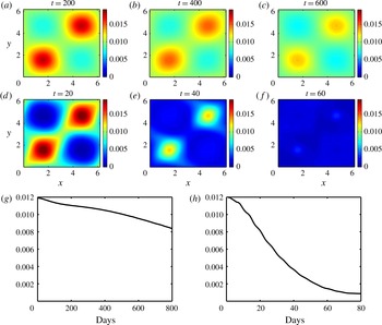
(a–c) Kinetic energy of the first 150 baroclinic modes integrated over the top 100 m of the model domain for the simulation with $\unicode[STIX]{x1D716}=0.0125$ at times $2.5/\unicode[STIX]{x1D716}$ , $5/\unicode[STIX]{x1D716}$ and $7.5/\unicode[STIX]{x1D716}$ . (d–f) Same for simulation with $\unicode[STIX]{x1D716}=0.125$ . Both cases show an accumulation of wave energy in anticyclonic regions ( $[0,\unicode[STIX]{x03C0}]\times [0,\unicode[STIX]{x03C0}]$ and $[\unicode[STIX]{x03C0},2\unicode[STIX]{x03C0}]\times [\unicode[STIX]{x03C0},2\unicode[STIX]{x03C0}]$ for the streamfunction (2.7)), with stronger accumulation in the case of larger $\unicode[STIX]{x1D716}$ . (g,h) Horizontally averaged and vertically integrated kinetic energy in the top 100 m of the model domain for simulations with $\unicode[STIX]{x1D716}=0.0125$ (g) and $\unicode[STIX]{x1D716}=0.125$ (h).

Figure 3.

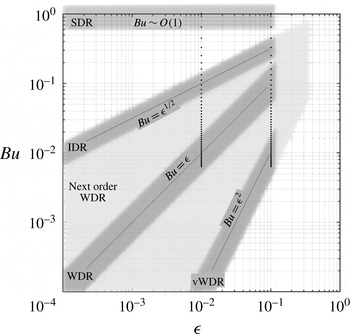
Dispersion regimes for rotating shallow water. The dark grey regions denote the four subregimes developed in § 3; boundaries of each region are fuzzy, to emphasize that the regions are not precisely defined. The region at the top is SDR, with $Bu\sim O(1)$ , and the region along the diagonal is WDR: the YBJ regime, with $Bu\sim \unicode[STIX]{x1D716}$ . The subregimes IDR ( $Bu\sim \unicode[STIX]{x1D716}^{1/2}$ ) and vWDR ( $Bu\sim \unicode[STIX]{x1D716}^{2}$ ) are also shown. The WDR region is bound on the right by $\unicode[STIX]{x1D716}\approx 10^{-1}$ , as a canonical small value. The light grey region denotes the next-order WDR equation (3.17), bounded by $Bu\sim \unicode[STIX]{x1D716}^{2}$ and $Bu\sim \unicode[STIX]{x1D716}^{1/2}$ , capturing all possible balances of terms in the equation. The right side boundary is $\unicode[STIX]{x1D716}\approx 10^{-1/2}$ , so that the smallest terms, which scale like $\unicode[STIX]{x1D716}^{2}\approx 10^{-1}$ , are still ‘small’. The vertical dotted lines represent values of $Bu_{n}$ for $n=1,\ldots ,50$ , $L=40$ km, $f=10^{-4}~\text{s}^{-1}$ , $N=100f$ and $H=5$  km, at two different values of $\unicode[STIX]{x1D716}$ . The point is to show the range of regimes necessary to describe how the problem changes with Rossby number.

Figure 2(a–f) shows the horizontal distribution of wave kinetic energy, integrated vertically over the top 100 m for each of the two simulations, at times $2.5/\unicode[STIX]{x1D716}$ , $5/\unicode[STIX]{x1D716}$ and $7.5/\unicode[STIX]{x1D716}$ (normalized by their respective Rossby numbers). One can immediately see, especially in the larger Rossby number case (d–f), an expulsion of wave energy from cyclonic vorticity regions of the background flow and trapping of waves in anticyclonic vorticity regions. The wave energy is redistributed both horizontally into anticyclonic regions, and downward, as can be seen in panels (g,h), which show time series of the horizontally averaged and vertically integrated kinetic energy in the upper 100  m for each simulation. In the larger Rossby number case, after 80 days almost $93\,\%$ of the initial energy has left the top 100 m, whereas after an order of magnitude longer time (800 days), only $29\,\%$ of the initial energy leaves the upper ocean for the case $\unicode[STIX]{x1D716}=0.0125$ . This is the ‘inertial chimney effect’ (Lee & Niiler Reference Lee and Niiler1998), the mechanism by which anticyclonic vorticity regions act as conduits for inertial energy to reach the thermocline. We note that we were able to obtain this phenomenon, consistently observed in numerical simulations using more complex models (Zhai, Greatbatch & Zhao Reference Zhai, Greatbatch and Zhao2005; Zhai, Greatbatch & Eden Reference Zhai, Greatbatch and Eden2007), in the most basic set-up – using linearized interaction equations.

The stronger tendency for anticyclonic accumulation and downward wave energy propagation for the case with $\unicode[STIX]{x1D716}=0.125$ is consistent with the inference from figure 1 that with larger Rossby number, more modes satisfy $Bu_{n}\ll 1$ , which suppresses the dispersive pressure term in the leading-order dynamics, resulting in strong modulation of NIWs by the background flow and rapid vertical propagation. For smaller Rossby numbers, most of the wave energy is in modes that satisfy $Bu_{n}\sim O(1)$ leading to less modulation and thus weaker vertical propagation of NIWs.

To capture these dynamics, we consider two broad scalings: (i) the ‘strong dispersion regime’ (SDR) with $Bu_{n}\sim O(1)$ and (ii) the ‘weak dispersion regime’ (WDR) with $Bu_{n}\ll 1$ , with names motivated by terminology introduced in Danioux & Klein (Reference Danioux and Klein2008) and discussed below (1.8). The latter regime, which Klein & Llewellyn Smith (Reference Klein and Llewellyn Smith2001) also identify as the ‘trapping regime’, was investigated in detail by YBJ.

Notice that for very small Rossby numbers, there may also be modes with $Bu_{n}$ that are asymptotically small but still large compared to $\unicode[STIX]{x1D716}$ . Moreover, for larger Rossby numbers, there may be modes with $Bu_{n}\sim O(\unicode[STIX]{x1D716}^{2})$ . This can be seen in figure 3, which attempts to delineate the asymptotic regimes discussed above, as well as some new subregimes. The vertical dotted lines represent $Bu_{n}$ for $n=1$ – $50$ , with the same parameters used in the analysis above, for two different values of $\unicode[STIX]{x1D716}$ . One can see that in both cases, there are many modes that do not lie within the formal ranges of validity of the SDR or WDR. However, we will show in the next section that a next-order expansion about the distinguished limit $Bu_{n}\sim \unicode[STIX]{x1D716}$ provides correction terms for the cases where $Bu_{n}$ , while still small, is asymptotically large or small compared to $\unicode[STIX]{x1D716}$ , as denoted by the lighter grey region called ‘next order WDR’. At the edges of this regime are subregimes defined by $Bu_{n}\sim \unicode[STIX]{x1D716}^{1/2}$ and $Bu_{n}\sim \unicode[STIX]{x1D716}^{2}$ , which we refer to, respectively, as the ‘intermediate dispersion regime’ (IDR) and ‘very weak dispersion regime’ (vWDR). For larger $\unicode[STIX]{x1D716}$ , most modes lie deep in the WDR, and span both its subregimes, IDR and vWDR. For smaller $\unicode[STIX]{x1D716}$ , more modes lie in the IDR. Details of these limiting cases will be discussed in § 3.

3 Amplitude equations for strong and weak dispersion regimes

Here we consider asymptotic approaches to understanding the range of behaviours for different vertical modes seen in the last section. Keeping in mind that the following analysis holds for specific baroclinic modes, we suppress the subscript $n$ ; for instance we represent modal Burger number as $Bu$ instead of $Bu_{n}$ , wave amplitude as $A$ instead of $A_{n}$ and so on. We rewrite (1.6) as

(3.1a ) $$\begin{eqnarray}\displaystyle & \displaystyle \frac{\unicode[STIX]{x2202}\boldsymbol{v}}{\unicode[STIX]{x2202}t}+\hat{\boldsymbol{z}}\times \boldsymbol{v}+Bu\unicode[STIX]{x1D735}p+\unicode[STIX]{x1D716}\left\{\boldsymbol{v}\boldsymbol{\cdot }\unicode[STIX]{x1D735}\boldsymbol{V}+\boldsymbol{V}\boldsymbol{\cdot }\unicode[STIX]{x1D735}\boldsymbol{v}\right\}=0, & \displaystyle\end{eqnarray}$$

(3.1b ) $$\begin{eqnarray}\displaystyle & \displaystyle \frac{\unicode[STIX]{x2202}p}{\unicode[STIX]{x2202}t}+\unicode[STIX]{x1D735}\boldsymbol{\cdot }\boldsymbol{v}+\unicode[STIX]{x1D716}~\boldsymbol{V}\boldsymbol{\cdot }\unicode[STIX]{x1D735}p=0. & \displaystyle\end{eqnarray}$$

(3.2a,b ) $$\begin{eqnarray}u=\text{constant},\quad v=p=0\quad \text{at}\quad t=0\end{eqnarray}$$

so that spatially homogeneous inertial oscillations are excited. Because the analysis that follows assumes a single length scale for the background flow, we use the idealized streamfunction (2.7), representing a single dominant mode of the background flow.

Using the method of multiple time scales, in the coming subsections we derive amplitude equations for NIW modes with different $Bu$ – $\unicode[STIX]{x1D716}$ scalings. We note that although we assume a steady mean flow throughout, the derivation of the amplitude equations requires only a time scale separation between the mean flow and NIWs  and therefore the derivations retain their validity if the mean flow is slowly evolving rather than steady. These amplitude equations will be compared with numerical solutions to the linear rotating shallow water equations, (3.1) (hereafter RSW). As with the linear Boussinesq simulation discussed in § 2, the codes used to solve the linear shallow water equations were pseudospectral with fourth-order Runge–Kutta time stepping. A hyperdiffusion operator of the form $-\unicode[STIX]{x1D708}\unicode[STIX]{x0394}^{4}\boldsymbol{v}$ was added to the momentum equations in the shallow water equations, and to the amplitude equations in various regimes for numerical stability. The resolution necessary for convergence of the numerical solutions varied based on the asymptotic regime considered. For example $256^{2}$ or $512^{2}$ Fourier modes were necessary in order to capture the formation of small-scale features in vWDR whereas $128^{2}$ Fourier modes were sufficient in other regimes. Hyperviscosity was varied according to the resolution so as to obtain $O(1)$ Reynolds number at the grid scale, with $\unicode[STIX]{x1D708}=10^{-12}$ at lowest resolution. Convergence was checked by doubling the resolution and decreasing the time steps.

3.1 The weak dispersion regime

‘Weak dispersion’ refers to the suppression of the pressure term (which leads to wave dispersion) at leading order in (3.1a ) when $Bu\ll 1$ . This defines the broad set of dynamics that, as argued above, characterizes higher baroclinic modes. For expository reasons, we discuss this regime first, and the low-mode case of $Bu\sim O(1)$ later. To proceed asymptotically in the weak dispersion regime, one needs to assume a particular scaling between $Bu$ and the defining small parameter, $\unicode[STIX]{x1D716}$ . YBJ exploited the distinguished limit $Bu\sim O(\unicode[STIX]{x1D716})$ to derive an amplitude equation for the evolution of NIWs. We consider the same scaling to derive an improved equation for the weak dispersion regime, noting that this distinguished scaling retains the largest number of terms entering at asymptotically higher orders.

Following YBJ, it is convenient to switch to complex coordinates

(3.3a,b ) $$\begin{eqnarray}\mathscr{U}=u+\text{i}v\quad \text{and}\quad \unicode[STIX]{x1D709}=x+\text{i}y\end{eqnarray}$$

from which it follows that $\unicode[STIX]{x2202}/\unicode[STIX]{x2202}x+\text{i}\unicode[STIX]{x2202}/\unicode[STIX]{x2202}y=2\unicode[STIX]{x2202}/\unicode[STIX]{x2202}\unicode[STIX]{x1D709}^{\ast }$ , $U+\text{i}V=2\text{i}\,\unicode[STIX]{x2202}\unicode[STIX]{x1D6F9}/\unicode[STIX]{x2202}\unicode[STIX]{x1D709}^{\ast }$ , $\unicode[STIX]{x1D735}\boldsymbol{\cdot }\boldsymbol{v}=\unicode[STIX]{x2202}\mathscr{U}/\unicode[STIX]{x2202}\unicode[STIX]{x1D709}\,+\text{c.c.}$ and $\boldsymbol{v}\boldsymbol{\cdot }\unicode[STIX]{x1D735}=\mathscr{U}\unicode[STIX]{x2202}/\unicode[STIX]{x2202}\unicode[STIX]{x1D709}\,+\text{c.c.}$ For convenience later, we also define the operators

(3.4a,b ) $$\begin{eqnarray}\unicode[STIX]{x0394}\equiv \frac{\unicode[STIX]{x2202}^{2}}{\unicode[STIX]{x2202}x^{2}}+\frac{\unicode[STIX]{x2202}^{2}}{\unicode[STIX]{x2202}y^{2}}=4\frac{\unicode[STIX]{x2202}^{2}}{\unicode[STIX]{x2202}\unicode[STIX]{x1D709}\unicode[STIX]{x2202}\unicode[STIX]{x1D709}^{\ast }}\quad \text{and}\quad \unicode[STIX]{x0394}^{\bot }\equiv \frac{\unicode[STIX]{x2202}^{2}}{\unicode[STIX]{x2202}x^{2}}-\frac{\unicode[STIX]{x2202}^{2}}{\unicode[STIX]{x2202}y^{2}}+2\text{i}\frac{\unicode[STIX]{x2202}^{2}}{\unicode[STIX]{x2202}x\unicode[STIX]{x2202}y}=4\frac{\unicode[STIX]{x2202}^{2}}{\unicode[STIX]{x2202}{\unicode[STIX]{x1D709}^{\ast }}^{2}},\end{eqnarray}$$

the first of which is just the horizontal Laplacian. For the second operator we note a physical interpretation by observing that

(3.5) $$\begin{eqnarray}{|\unicode[STIX]{x0394}^{\bot }\unicode[STIX]{x1D6F9}|}^{2}=\left(\frac{\unicode[STIX]{x2202}^{2}\unicode[STIX]{x1D6F9}}{\unicode[STIX]{x2202}x^{2}}-\frac{\unicode[STIX]{x2202}^{2}\unicode[STIX]{x1D6F9}}{\unicode[STIX]{x2202}y^{2}}\right)^{2}+4\left(\frac{\unicode[STIX]{x2202}^{2}\unicode[STIX]{x1D6F9}}{\unicode[STIX]{x2202}x\unicode[STIX]{x2202}y}\right)^{2}=\left(\frac{\unicode[STIX]{x2202}V}{\unicode[STIX]{x2202}x}+\frac{\unicode[STIX]{x2202}U}{\unicode[STIX]{x2202}y}\right)^{2}+\left(\frac{\unicode[STIX]{x2202}U}{\unicode[STIX]{x2202}x}-\frac{\unicode[STIX]{x2202}V}{\unicode[STIX]{x2202}y}\right)^{2}=\unicode[STIX]{x1D70E}^{2},\end{eqnarray}$$

where $\unicode[STIX]{x1D70E}$ is the total mean horizontal shear (containing normal and tangential components). We also define the slow advection operator

(3.6) $$\begin{eqnarray}\frac{\text{D}}{\text{D}T}=\frac{\unicode[STIX]{x2202}}{\unicode[STIX]{x2202}T}+\boldsymbol{V}\boldsymbol{\cdot }\unicode[STIX]{x1D735}=\frac{\unicode[STIX]{x2202}}{\unicode[STIX]{x2202}T}+J(\unicode[STIX]{x1D6F9},~).\end{eqnarray}$$

Letting $T=\unicode[STIX]{x1D716}t$ be the slow time so that time derivatives become $\unicode[STIX]{x2202}/\unicode[STIX]{x2202}t\rightarrow \unicode[STIX]{x2202}/\unicode[STIX]{x2202}t+\unicode[STIX]{x1D716}\unicode[STIX]{x2202}/\unicode[STIX]{x2202}T$ , we add the $u$ equation to $\text{i}$ times the $v$ equation in (3.1a ) to obtain

(3.7a ) $$\begin{eqnarray}\displaystyle & \displaystyle \frac{\unicode[STIX]{x2202}\mathscr{U}}{\unicode[STIX]{x2202}t}+\text{i}\mathscr{U}+\unicode[STIX]{x1D716}\left[\frac{\text{D}\mathscr{U}}{\text{D}T}+\frac{\text{i}}{2}\left(\unicode[STIX]{x0394}\unicode[STIX]{x1D6F9}~\mathscr{U}+\unicode[STIX]{x0394}^{\bot }\unicode[STIX]{x1D6F9}~\mathscr{U}^{\ast }\right)+2\frac{Bu}{\unicode[STIX]{x1D716}}\frac{\unicode[STIX]{x2202}p}{\unicode[STIX]{x2202}\unicode[STIX]{x1D709}^{\ast }}\right]=0, & \displaystyle\end{eqnarray}$$

(3.7b ) $$\begin{eqnarray}\displaystyle & \displaystyle \frac{\unicode[STIX]{x2202}p}{\unicode[STIX]{x2202}t}+\frac{\unicode[STIX]{x2202}\mathscr{U}}{\unicode[STIX]{x2202}\unicode[STIX]{x1D709}}+\frac{\unicode[STIX]{x2202}\mathscr{U}^{\ast }}{\unicode[STIX]{x2202}\unicode[STIX]{x1D709}^{\ast }}+\unicode[STIX]{x1D716}\frac{\text{D}p}{\text{D}T}=0. & \displaystyle\end{eqnarray}$$

Expanding variables as

(3.8) $$\begin{eqnarray}(\mathscr{U},p)=(\mathscr{U}_{0},p_{0})+\unicode[STIX]{x1D716}(\mathscr{U}_{1},p_{1})+\unicode[STIX]{x1D716}^{2}(\mathscr{U}_{2},p_{2})+\cdots\end{eqnarray}$$

the leading-order equations are

(3.9a ) $$\begin{eqnarray}\displaystyle & \displaystyle \frac{\unicode[STIX]{x2202}\mathscr{U}_{0}}{\unicode[STIX]{x2202}t}+\text{i}\mathscr{U}_{0}=0, & \displaystyle\end{eqnarray}$$

(3.9b ) $$\begin{eqnarray}\displaystyle & \displaystyle \frac{\unicode[STIX]{x2202}p_{0}}{\unicode[STIX]{x2202}t}+\frac{\unicode[STIX]{x2202}\mathscr{U}_{0}}{\unicode[STIX]{x2202}\unicode[STIX]{x1D709}}+\frac{\unicode[STIX]{x2202}\mathscr{U}_{0}^{\ast }}{\unicode[STIX]{x2202}\unicode[STIX]{x1D709}^{\ast }}=0, & \displaystyle\end{eqnarray}$$

which have solutions

(3.10a,b ) $$\begin{eqnarray}\mathscr{U}_{0}=A_{0}\text{e}^{-\text{i}t},\quad p_{0}=-\text{i}\frac{\unicode[STIX]{x2202}A_{0}}{\unicode[STIX]{x2202}\unicode[STIX]{x1D709}}\text{e}^{-\text{i}t}+\text{c.c.}\end{eqnarray}$$

where $A_{0}=A_{0}(\unicode[STIX]{x1D709},\unicode[STIX]{x1D709}^{\ast },T)$ . Using the leading-order solutions (3.10a,b ), the equations at $O(\unicode[STIX]{x1D716})$ are

(3.11a ) $$\begin{eqnarray}\displaystyle & & \displaystyle \frac{\unicode[STIX]{x2202}\mathscr{U}_{1}}{\unicode[STIX]{x2202}t}+\text{i}\mathscr{U}_{1}+\left[\frac{\text{D}A_{0}}{\text{D}T}+\frac{\text{i}}{2}\left(\unicode[STIX]{x0394}\unicode[STIX]{x1D6F9}~A_{0}-\frac{Bu}{\unicode[STIX]{x1D716}}\unicode[STIX]{x0394}A_{0}\right)\right]\text{e}^{-\text{i}t}\nonumber\\ \displaystyle & & \displaystyle \qquad +\,\frac{\text{i}}{2}\left[\unicode[STIX]{x0394}^{\bot }\unicode[STIX]{x1D6F9}~A_{0}^{\ast }+\frac{Bu}{\unicode[STIX]{x1D716}}~\unicode[STIX]{x0394}^{\bot }A_{0}^{\ast }\right]\text{e}^{\text{i}t}=0,\end{eqnarray}$$

(3.11b ) $$\begin{eqnarray}\displaystyle & & \displaystyle \frac{\unicode[STIX]{x2202}p_{1}}{\unicode[STIX]{x2202}t}+\frac{\unicode[STIX]{x2202}\mathscr{U}_{1}}{\unicode[STIX]{x2202}\unicode[STIX]{x1D709}}+\frac{\unicode[STIX]{x2202}\mathscr{U}_{1}^{\ast }}{\unicode[STIX]{x2202}\unicode[STIX]{x1D709}^{\ast }}+\frac{\text{D}}{\text{D}T}\left(-\text{i}\frac{\unicode[STIX]{x2202}A_{0}}{\unicode[STIX]{x2202}\unicode[STIX]{x1D709}}\text{e}^{-\text{i}t}+\text{c.c.}\right)=0.\end{eqnarray}$$

Eliminating secular growth in (3.11a ) by setting to zero the terms multiplied by $\text{e}^{-\text{i}t}$ , we obtain the shallow water version of the YBJ amplitude equation

(3.12) $$\begin{eqnarray}\frac{\unicode[STIX]{x2202}A_{0}}{\unicode[STIX]{x2202}T}+J(\unicode[STIX]{x1D6F9},A_{0})+\frac{\text{i}}{2}\left((\unicode[STIX]{x0394}\unicode[STIX]{x1D6F9})A_{0}-\frac{Bu}{\unicode[STIX]{x1D716}}\unicode[STIX]{x0394}A_{0}\right)=0.\end{eqnarray}$$

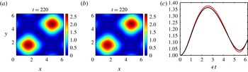
Note that in the slow time $T$ , all terms in this expression are of the same asymptotic order; when $T=\unicode[STIX]{x1D716}t$ is used, all terms except the time derivative are of $O(\unicode[STIX]{x1D716})$ . Figure 4 compares the numerical solution of (3.12) with that of RSW for $Bu=\unicode[STIX]{x1D716}=0.0125$ . The amplitude equation agrees quite well with the parent model in detail. Note also the expected accumulation of wave activity in regions of anticyclonic vorticity.

Figure 4.

(a,b) $|A|=\sqrt{u^{2}+v^{2}}$ obtained from the YBJ equation (3.12) and from RSW (3.1). (c)  $\sqrt{\langle |A|^{2}\rangle ^{part}}$ versus slow time, $\unicode[STIX]{x1D716}t$ , for the YBJ amplitude equation (red curve) and for RSW (black curve) where $\langle \unicode[STIX]{x1D719}\rangle ^{part}$ refers to spatial average calculated over the top right quarter of the domain. The simulations used the parameters $\unicode[STIX]{x1D716}=Bu=0.0125$ .

3.2 Next-order weak dispersion regimes

Here we continue to the next order in $\unicode[STIX]{x1D716}$ to provide an amplitude equation that allows for a wider range of scalings between the Burger and Rossby numbers, consistent with the results in § 2. The usefulness of this exercise will be demonstrated after the derivation.

We will first need the solution to (3.11), given $A_{0}$ from (3.12). The result is

(3.12a,b ) $$\begin{eqnarray}\displaystyle \mathscr{U}_{1}=A_{1}\text{e}^{-\text{i}t}+B_{1}\text{e}^{\text{i}t},\quad p_{1}=-\left[\text{i}\left(\frac{\unicode[STIX]{x2202}A_{1}}{\unicode[STIX]{x2202}\unicode[STIX]{x1D709}}+\frac{\unicode[STIX]{x2202}B_{1}^{\ast }}{\unicode[STIX]{x2202}\unicode[STIX]{x1D709}^{\ast }}\right)+\frac{\text{D}}{\text{D}T}\frac{\unicode[STIX]{x2202}A_{0}}{\unicode[STIX]{x2202}\unicode[STIX]{x1D709}}\right]\text{e}^{-\text{i}t}+\text{c.c.} & & \displaystyle\end{eqnarray}$$

where

(3.13) $$\begin{eqnarray}B_{1}=-\frac{1}{4}\left(\unicode[STIX]{x0394}^{\bot }\unicode[STIX]{x1D6F9}~A_{0}^{\ast }+\frac{Bu}{\unicode[STIX]{x1D716}}\unicode[STIX]{x0394}^{\bot }A_{0}^{\ast }\right).\end{eqnarray}$$

To obtain a higher-order amplitude equation, we employ a ‘composite’ technique that proceeds as follows. The solvability condition (3.12) is modified as

(3.14) $$\begin{eqnarray}\frac{\text{D}A_{0}}{\text{D}T}+\frac{\text{i}}{2}\left((\unicode[STIX]{x0394}\unicode[STIX]{x1D6F9})A_{0}-\frac{Bu}{\unicode[STIX]{x1D716}}\unicode[STIX]{x0394}A_{0}\right)=\unicode[STIX]{x1D716}\unicode[STIX]{x1D6F7},\end{eqnarray}$$

where $\unicode[STIX]{x1D6F7}=\unicode[STIX]{x1D6F7}(\boldsymbol{x},T)$ (or $\unicode[STIX]{x1D6F7}(\unicode[STIX]{x1D709},\unicode[STIX]{x1D709}^{\ast },T)$ in terms of complex coordinates) is a higher-order correction term. This is analogous to the derivation of higher-order correction terms for the nonlinear Schrödinger equation, which is the lower-order equation, to capture the evolution of deep water waves to a higher level of accuracy (see Dysthe Reference Dysthe1979; Trulsen & Dysthe Reference Trulsen and Dysthe1996). The reader may refer to Ablowitz (Reference Ablowitz2011) for similar problems that take advantage of this composite method. An alternative approach is to define a second slow time, $\unicode[STIX]{x1D70F}=\unicode[STIX]{x1D716}^{2}t$ and derive an amplitude equation on time scales $\unicode[STIX]{x1D70F}\sim O(1)$ . Such a strategy, it can be shown, is equivalent to the above method and would result in the same slow amplitude equation on $1/\unicode[STIX]{x1D716}^{2}$ time scales (see, for example, appendix A of Thomas (Reference Thomas2016) for a comparison of these two alternative methods). To obtain $\unicode[STIX]{x1D6F7}$ , we need to prevent secular growth at the next order. At $O(\unicode[STIX]{x1D716}^{2})$ , (3.7a ) gives

(3.15) $$\begin{eqnarray}\displaystyle \frac{\unicode[STIX]{x2202}\mathscr{U}_{2}}{\unicode[STIX]{x2202}t}+\text{i}\mathscr{U}_{2}+\unicode[STIX]{x1D6F7}\text{e}^{-\text{i}t}+\frac{\text{D}\mathscr{U}_{1}}{\text{D}T}+\frac{\text{i}}{2}\left(\unicode[STIX]{x0394}\unicode[STIX]{x1D6F9}\mathscr{U}_{1}+\unicode[STIX]{x0394}^{\bot }\unicode[STIX]{x1D6F9}\mathscr{U}_{1}^{\ast }\right)+2\frac{Bu}{\unicode[STIX]{x1D716}}\frac{\unicode[STIX]{x2202}p_{1}}{\unicode[STIX]{x2202}\unicode[STIX]{x1D709}^{\ast }}=0. & & \displaystyle\end{eqnarray}$$

Substituting the first-order solutions (3.12a,b ) into the above and setting terms proportional to $\text{e}^{-\text{i}t}$ to zero, we obtain the solvability condition

(3.16) $$\begin{eqnarray}\unicode[STIX]{x1D6F7}+\frac{\text{D}A_{1}}{\text{D}T}+\frac{\text{i}}{2}\left(\unicode[STIX]{x0394}\unicode[STIX]{x1D6F9}A_{1}+B_{1}^{\ast }\unicode[STIX]{x0394}^{\bot }\unicode[STIX]{x1D6F9}\right)-\frac{Bu}{2\unicode[STIX]{x1D716}}\left[\text{i}\unicode[STIX]{x0394}A_{1}+\text{i}\unicode[STIX]{x0394}^{\bot }B_{1}^{\ast }+4\frac{\unicode[STIX]{x2202}}{\unicode[STIX]{x2202}\unicode[STIX]{x1D709}^{\ast }}\left(\frac{\text{D}}{\text{D}T}\frac{\unicode[STIX]{x2202}A_{0}}{\unicode[STIX]{x2202}\unicode[STIX]{x1D709}}\right)\right]=0.\end{eqnarray}$$

We then eliminate $\unicode[STIX]{x1D6F7}$ by combining the two equations as (3.14) + $\unicode[STIX]{x1D716}$ (3.16), use (3.13) to eliminate $B_{1}$ , (3.12) to eliminate the $\unicode[STIX]{x2202}^{2}\!A_{0}/\unicode[STIX]{x2202}T\unicode[STIX]{x2202}\unicode[STIX]{x1D709}$ term and define a combined amplitude as $A=A_{0}+\unicode[STIX]{x1D716}A_{1}$ to obtain the composite amplitude equation

(3.17) $$\begin{eqnarray}\frac{\unicode[STIX]{x2202}A}{\unicode[STIX]{x2202}T}+J(\unicode[STIX]{x1D6F9},A)+\frac{\text{i}}{2}\unicode[STIX]{x0394}\unicode[STIX]{x1D6F9}A-\frac{Bu}{\unicode[STIX]{x1D716}}\frac{\text{i}}{2}\unicode[STIX]{x0394}A-\frac{\text{i}}{8}\frac{Bu^{2}}{\unicode[STIX]{x1D716}}\unicode[STIX]{x0394}^{2}A-\frac{\text{i}}{8}\unicode[STIX]{x1D716}|\unicode[STIX]{x0394}^{\bot }\unicode[STIX]{x1D6F9}|^{2}A+2BuG=0,\end{eqnarray}$$

where

(3.18) $$\begin{eqnarray}\displaystyle G=\frac{\unicode[STIX]{x2202}}{\unicode[STIX]{x2202}\unicode[STIX]{x1D709}^{\ast }}J\left(\frac{\unicode[STIX]{x2202}\unicode[STIX]{x1D6F9}}{\unicode[STIX]{x2202}\unicode[STIX]{x1D709}},A\right)+\text{i}\frac{\unicode[STIX]{x2202}^{2}}{\unicode[STIX]{x2202}{\unicode[STIX]{x1D709}^{\ast }}^{2}}\left(\frac{\unicode[STIX]{x2202}^{2}\unicode[STIX]{x1D6F9}}{\unicode[STIX]{x2202}\unicode[STIX]{x1D709}^{2}}A\right)-\text{i}\left(\frac{\unicode[STIX]{x2202}^{2}\unicode[STIX]{x1D6F9}}{\unicode[STIX]{x2202}{\unicode[STIX]{x1D709}^{\ast }}^{2}}\right)\frac{\unicode[STIX]{x2202}^{2}A}{\unicode[STIX]{x2202}\unicode[STIX]{x1D709}^{2}}+\frac{\text{i}}{8}\unicode[STIX]{x0394}\left(\unicode[STIX]{x0394}\unicode[STIX]{x1D6F9}A\right). & & \displaystyle\end{eqnarray}$$

We may further set $T=\unicode[STIX]{x1D716}t$ in (3.17) resulting in a multiplication of every term besides the time derivative by $\unicode[STIX]{x1D716}$ (likewise for (3.12)).

Notice that (3.17) contains all the terms from (3.12), in addition to new correction terms of orders $Bu^{2}/\unicode[STIX]{x1D716}$ , $\unicode[STIX]{x1D716}$ and $Bu$ . While typically one would seek a higher-order equation in order to extend the temporal range of validity of the model, or to improve accuracy at large values of the small parameter, here, we argue the most useful aspect of the extended model lies in it’s ‘off-axis’ improvements: $Bu$ can stray further from $\unicode[STIX]{x1D716}$ at fixed $\unicode[STIX]{x1D716}$ . Referring back to figure 3, the next-order WDR model captures more of the dynamics sampled by a spectrum of waves (a range of $Bu_{n}$ ) at a given $\unicode[STIX]{x1D716}$ . Consistent with this goal, we want to keep some correction terms, but we see no reason to use the full expression with the exact choice $Bu=\unicode[STIX]{x1D716}$ , for which the YBJ equation (3.12) was shown in the previous subsection to match the RSW solutions extremely well. Thus rather than use this equation as derived, we now proceed to consider two subranges.

Consider separately examples for the cases (i)  $1\gg Bu\gg \unicode[STIX]{x1D716}$ (e.g. $Bu\sim \unicode[STIX]{x1D716}^{1/2}$ ), (ii)  $Bu\sim \unicode[STIX]{x1D716}$ and (iii)  $\unicode[STIX]{x1D716}\gg Bu$ (e.g. $Bu\sim \unicode[STIX]{x1D716}^{2}$ ). The terms with prefactors in (3.17) then scale as

(3.19) $$\begin{eqnarray}\displaystyle \left.\begin{array}{@{}c@{}}\displaystyle (\text{i})~Bu\sim \unicode[STIX]{x1D716}^{1/2}:~\frac{Bu}{\unicode[STIX]{x1D716}}\sim \unicode[STIX]{x1D716}^{-1/2}\gg \frac{Bu^{2}}{\unicode[STIX]{x1D716}}\sim 1\gg Bu\sim \unicode[STIX]{x1D716}^{1/2}\gg \unicode[STIX]{x1D716},\\ \displaystyle (\text{ii})~Bu\sim \unicode[STIX]{x1D716}:~\frac{Bu}{\unicode[STIX]{x1D716}}\sim 1\gg \frac{Bu^{2}}{\unicode[STIX]{x1D716}}\sim Bu\sim \unicode[STIX]{x1D716},\\ \displaystyle (\text{iii})~Bu\sim \unicode[STIX]{x1D716}^{2}:~\frac{Bu}{\unicode[STIX]{x1D716}}\sim \unicode[STIX]{x1D716}\gg Bu\sim \unicode[STIX]{x1D716}^{2}\gg \frac{Bu^{2}}{\unicode[STIX]{x1D716}}\sim \unicode[STIX]{x1D716}^{3}.\end{array}\right\} & & \displaystyle\end{eqnarray}$$

In case (i), the new $Bu^{2}/\unicode[STIX]{x1D716}$ term is $O(1)$ and the $Bu/\unicode[STIX]{x1D716}$ term (part of the original YBJ equation) is dominant. The other two terms, both new, are negligible. In case (ii), the three new terms, including $Bu\,G$ , are all $O(\unicode[STIX]{x1D716})$ and small compared to the $O(1)$ original term $Bu/\unicode[STIX]{x1D716}$ . As mentioned above, there is little reason to retain these terms since the original WDR equation was already shown to be accurate. Finally, in case (iii), all terms are small, but the new term, with prefactor $\unicode[STIX]{x1D716}$ in (3.17), is of the same order as the original term $Bu/\unicode[STIX]{x1D716}$ , and so should be retained. Below we consider cases (i) and (iii) explicitly.

3.2.1 Intermediate dispersion regime: $Bu\sim \sqrt{\unicode[STIX]{x1D716}}$

Recall from figure 1 that the modal Burger number decreases monotonically as the mode $n$ increases. For sufficiently small $\unicode[STIX]{x1D716}$ , some modal Burger numbers satisfy $\unicode[STIX]{x1D716}\ll Bu_{n}\ll 1$ , and the number of modes satisfying this scaling increases with decreasing $\unicode[STIX]{x1D716}$ . This motivates the scaling $Bu\sim \sqrt{\unicode[STIX]{x1D716}}$ , which we term the ‘intermediate dispersion regime’. In this limit, the pressure gradient term in (1.6a ) is small, and so does not appear at leading order, but is larger than the mean flow interaction terms. We set $Bu\sim \sqrt{\unicode[STIX]{x1D716}}$ , set $T=\unicode[STIX]{x1D716}t$ and retain terms up to $O(\unicode[STIX]{x1D716})$ in (3.17) to get the ‘intermediate dispersion regime’ (IDR) amplitude equation

(3.20) $$\begin{eqnarray}\frac{\unicode[STIX]{x2202}A}{\unicode[STIX]{x2202}t}+\unicode[STIX]{x1D716}J(\unicode[STIX]{x1D6F9},A)+\unicode[STIX]{x1D716}\frac{\text{i}}{2}(\unicode[STIX]{x0394}\unicode[STIX]{x1D6F9})A-Bu\frac{\text{i}}{2}\unicode[STIX]{x0394}A-Bu^{2}\frac{\text{i}}{8}\unicode[STIX]{x0394}^{2}A=0.\end{eqnarray}$$

Alternatively, we could have obtained the above amplitude equation by beginning with the scaling $Bu\sim \sqrt{\unicode[STIX]{x1D716}}$ in RSW and using multiscale asymptotic analysis as before with $\sqrt{\unicode[STIX]{x1D716}}$ as the small parameter. Note that the above equation has two dispersive terms: the higher-order dispersive term, $\unicode[STIX]{x0394}^{2}A$ , which is of the same order as the advection and refraction terms (since $Bu\sim \sqrt{\unicode[STIX]{x1D716}}$ ), is asymptotically smaller than the lower-order dispersive term, $\unicode[STIX]{x0394}A$ , but is expected to be an important correction on $1/\unicode[STIX]{x1D716}$ time scales.

If we ignore the mean flow terms, the dispersion relationship for the above equation has the form $\unicode[STIX]{x1D714}_{idr}=(Bu/2)|\boldsymbol{k}|^{2}-(Bu^{2}/8)|\boldsymbol{k}|^{4}$ . Further if we Taylor expand the dispersion relationship of gravity waves assuming small Burger number, we obtain

(3.21) $$\begin{eqnarray}\sqrt{1+Bu|\boldsymbol{k}|^{2}}\sim 1+\frac{Bu}{2}|\boldsymbol{k}|^{2}-\frac{Bu^{2}}{8}|\boldsymbol{k}|^{4}.\end{eqnarray}$$

Note that the ‘1’ above is associated with the pure inertial frequency part, which was removed by deriving the slowly evolving amplitude equation. Therefore, the higher-order dispersion term in (3.20) corresponds to the dispersive term expected according to the gravity wave dispersion relationship.

To see the improvement obtained by the addition of the higher-order dispersion term in IDR, we set $\unicode[STIX]{x1D716}=0.0125$ and $Bu=\sqrt{\unicode[STIX]{x1D716}}$ and compute numerical solutions of the IDR amplitude equation (3.20), the YBJ equation (3.12) and RSW (3.1). We define the error relative to RSW as

(3.22) $$\begin{eqnarray}e_{idr}=\frac{\left\langle |A_{idr}-A_{rsw}|^{2}\right\rangle }{\left\langle |A_{rsw}|^{2}\right\rangle },\end{eqnarray}$$

where $\langle \,\rangle$ denotes spatial averaging, $A_{rsw}=\sqrt{u^{2}+v^{2}}$ is obtained from the numerical solution of (3.1) and $A_{idr}$ is the wave amplitude obtained from the numerical solution of (3.20). Replacing ‘ $idr$ ’ with ‘ $ybj$ ’ indicates the equivalent error for the YBJ equation (3.12) relative to RSW. The results are given in figure 5, panel (a) of which shows the amplitude modulus $|A|=\sqrt{u^{2}+v^{2}}$ for IDR, YBJ and RSW at $\unicode[STIX]{x1D716}t=6.25$ .

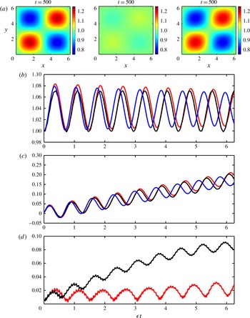
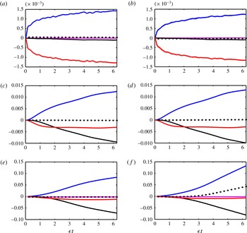
Figure 5(b) shows the (root mean square) r.m.s. velocity in the top right quarter of the domain while figure 5(c) shows the phase of the wave field calculated based on the average velocities in the top right quarter of the domain. We find that although the magnitudes of the velocity predicted by IDR and YBJ equations are comparable, as can be inferred from figure 5(b), the YBJ solution becomes out of phase with RSW solution, the difference increasing with time. This is clearly seen figure 5(c) that shows the phase. Observe that for small times, all three models agree in phase and are indistinguishable. However, on longer time scales the YBJ equation deviates significantly from the RSW solution while the IDR solution diverges only slightly. 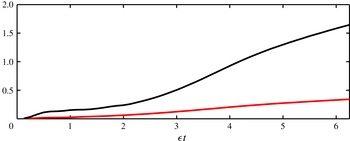At slow time $T=\unicode[STIX]{x1D716}t=6.25$ , when YBJ and RSW are almost completely out of phase, figure 5(a) shows the horizontal structure of the velocity field. Observe that while RSW predicts a wave field with increased concentration in anticyclones and decreased concentration in cyclones, a behaviour that is well captured by the IDR equation, the YBJ equation predicts an almost homogeneous wave field at this time. Finally the last panel shows the r.m.s. error between YBJ and IDR equations as compared with RSW. As can be seen, the error of the YBJ equation increases at a much more rapid rate than that for the IDR equation.

Figure 5.

(a)  $|A|=\sqrt{u^{2}+v^{2}}$ for IDR, YBJ and RSW at $\unicode[STIX]{x1D716}t=6.25$ . (b)  $\sqrt{\langle |A|^{2}\rangle ^{part}}$ (spatial average over top right quarter) obtained from RSW (black), YBJ (blue) and IDR (red). (c) Phase ( $\unicode[STIX]{x1D703}$ , calculated as $\langle A\rangle ^{part}=R\text{e}^{\text{i}\unicode[STIX]{x1D703}}$ ) of various models with the same colour pattern as the second panel. (d) Errors $e_{idr}$ (red curve, see (3.22)) and $e_{ybj}$ (black curve). All the simulations used the parameters $Bu=\sqrt{\unicode[STIX]{x1D716}},\unicode[STIX]{x1D716}=0.0125$ .

3.2.2 Very weak dispersion regime: $Bu\sim \unicode[STIX]{x1D716}^{2}$

We now consider very high baroclinic modes, in a regime characterized by $Bu\sim \unicode[STIX]{x1D716}^{2}$ . Wave dispersion in this regime is smaller than the mean flow interaction terms and we therefore call this the ‘very weak dispersion regime’. Setting $Bu\sim \unicode[STIX]{x1D716}^{2}$ and retaining terms up to $O(\unicode[STIX]{x1D716}^{2})$ in (3.17), we obtain the vWDR amplitude equation

(3.23) $$\begin{eqnarray}\frac{\unicode[STIX]{x2202}A}{\unicode[STIX]{x2202}t}+\unicode[STIX]{x1D716}J(\unicode[STIX]{x1D6F9},A)+\unicode[STIX]{x1D716}\frac{\text{i}}{2}(\unicode[STIX]{x0394}\unicode[STIX]{x1D6F9})A-Bu\frac{\text{i}}{2}\unicode[STIX]{x0394}A-\unicode[STIX]{x1D716}^{2}~\frac{\text{i}}{8}|\unicode[STIX]{x0394}^{\bot }\unicode[STIX]{x1D6F9}|^{2}A=0.\end{eqnarray}$$

As in IDR, we note that rather than considering a limiting form of (3.17) we could have obtained the above equation starting from RSW by setting $Bu\sim \unicode[STIX]{x1D716}^{2}$ . If we ignore the dispersive and advective terms, we observe that the solution of the amplitude equation may be written as

(3.24) $$\begin{eqnarray}A=A(t=0)\exp \left\{-\text{i}t\left(\frac{\unicode[STIX]{x1D716}}{2}\unicode[STIX]{x0394}\unicode[STIX]{x1D6F9}-\frac{\unicode[STIX]{x1D716}^{2}}{8}\unicode[STIX]{x1D70E}^{2}\right)\right\},\end{eqnarray}$$

which indicates that the geostrophic vorticity and shear, $\unicode[STIX]{x1D70E}$ (see (3.5)), shift the frequency of the wave field. Previous works have identified this by simply ignoring the pressure gradient term in RSW right from the start and calculating the frequency shift produced by a mean flow, two notable ones being Fomin (Reference Fomin1973) and Chavanne, Firing & Ascani (Reference Chavanne, Firing and Ascani2012). Chavanne et al. (Reference Chavanne, Firing and Ascani2012) finds an expression for effective frequency due to the modulation by a mean flow as (equation (A 5) there):

(3.25) $$\begin{eqnarray}\displaystyle \frac{f_{eff}}{f}=\left\{1+\unicode[STIX]{x1D716}\unicode[STIX]{x0394}\unicode[STIX]{x1D6F9}+\frac{\unicode[STIX]{x1D716}^{2}}{4}\left(\unicode[STIX]{x0394}\unicode[STIX]{x1D6F9}-\unicode[STIX]{x1D70E}^{2}\right)\right\}^{1/2}\sim 1+\frac{\unicode[STIX]{x1D716}}{2}\unicode[STIX]{x0394}\unicode[STIX]{x1D6F9}-\frac{\unicode[STIX]{x1D716}^{2}}{8}\unicode[STIX]{x1D70E}^{2}+O(\unicode[STIX]{x1D716}^{3}), & & \displaystyle\end{eqnarray}$$

which after removing the ‘1’ agrees with our expression in (3.24). The vWDR amplitude equation (3.23) therefore captures the next-order refraction term due to geostrophic shear in addition to the contribution from vorticity.

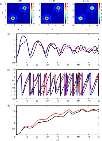
Since the wave dispersion is very weak in this regime, evolution of the wave field is even slower than for the other regimes. We therefore choose a higher Rossby number, $\unicode[STIX]{x1D716}=0.125$ , to facilitate long-time simulations. We now compare the vWDR and YBJ amplitude equations with RSW. Figure 6(a) compares the spatial structure of $|A|$ obtained from these three models. Figure 6(b,c) shows the r.m.s. and phase of the wave field in the top right quarter of the domain, while figure 6(d) shows the r.m.s. error between the vWDR and YBJ equations relative to RSW. Overall we find two important results. First, the vWDR is characterized by smaller wave field features in comparison with the other two cases considered so far. The formation of small-scale features in the wave field results in deviations between the reduced models and RSW, the difference increasing with time. Although all three models agree for an initial period, the magnitude and phase of the reduced models deviate from the parent model. Second, we note that the higher-order refraction term that forms a correction term to YBJ in this regime does not improve the features of the YBJ model. While not apparent here, in the next section we show that, with or without this term, the amplitude equation breaks down faster than expected; scaling of the conservation law for the amplitude equation offers an explanation.

Figure 6.

(a)  $|A|=\sqrt{u^{2}+v^{2}}$ for vWDR, YBJ and RSW at $\unicode[STIX]{x1D716}t=6.25$ . (b)  $\sqrt{\langle |A|^{2}\rangle ^{part}}$ obtained from RSW (black), YBJ (blue) and vWDR (red). (c) Phase ( $\unicode[STIX]{x1D703}$ , calculated as $\langle A\rangle ^{part}=R\text{e}^{\text{i}\unicode[STIX]{x1D703}}$ ) of various models with the same colour pattern as (b). (d) Errors $e_{vwdr}$ (red curve) and $e_{ybj}$ (black curve). All the simulations used the parameters $Bu=\unicode[STIX]{x1D716}^{2},\unicode[STIX]{x1D716}=0.125$ .

3.3 The strong dispersion regime

Recall that low baroclinic modes may have $Bu\sim O(1)$ , explicitly violating the initial assumption of YBJ that the Burger and Rossby numbers are of the same order. Because there can be no resonant forcing of the leading-order equation in this case, low baroclinic modes remain unmodulated for time scales $t\sim 1/\unicode[STIX]{x1D716}$ . However, as we show, resonant modulation of the NIWs is possible at time scales $t\sim 1/\unicode[STIX]{x1D716}^{2}$ . We therefore define a slow time scale $T=\unicode[STIX]{x1D716}^{2}t$ and set $\unicode[STIX]{x2202}/\unicode[STIX]{x2202}t\rightarrow \unicode[STIX]{x2202}/\unicode[STIX]{x2202}t+\unicode[STIX]{x1D716}^{2}\unicode[STIX]{x2202}/\unicode[STIX]{x2202}T$ to rewrite (3.1) as

(3.26a ) $$\begin{eqnarray}\displaystyle & \displaystyle \frac{\unicode[STIX]{x2202}\boldsymbol{v}}{\unicode[STIX]{x2202}t}+\hat{\boldsymbol{z}}\times \boldsymbol{v}+Bu\unicode[STIX]{x1D735}p+\unicode[STIX]{x1D716}\left\{\boldsymbol{v}\boldsymbol{\cdot }\unicode[STIX]{x1D735}\boldsymbol{V}+\boldsymbol{V}\boldsymbol{\cdot }\unicode[STIX]{x1D735}\boldsymbol{v}\right\}+\unicode[STIX]{x1D716}^{2}\frac{\unicode[STIX]{x2202}\boldsymbol{v}}{\unicode[STIX]{x2202}T}=0, & \displaystyle\end{eqnarray}$$

(3.26b ) $$\begin{eqnarray}\displaystyle & \displaystyle \frac{\unicode[STIX]{x2202}p}{\unicode[STIX]{x2202}t}+\unicode[STIX]{x1D735}\boldsymbol{\cdot }\boldsymbol{v}+\unicode[STIX]{x1D716}~\boldsymbol{V}\boldsymbol{\cdot }\unicode[STIX]{x1D735}p+\unicode[STIX]{x1D716}^{2}\frac{\unicode[STIX]{x2202}p}{\unicode[STIX]{x2202}T}=0. & \displaystyle\end{eqnarray}$$

We now expand all variables as an asymptotic series in $\unicode[STIX]{x1D716}$ , with the notation

(3.27) $$\begin{eqnarray}(\boldsymbol{v},p)=(\boldsymbol{v}_{0},p_{0})+\unicode[STIX]{x1D716}(\boldsymbol{v}_{1},p_{1})+O(\unicode[STIX]{x1D716}^{2}).\end{eqnarray}$$

At $O(1)$ , (3.26) become

(3.28a ) $$\begin{eqnarray}\displaystyle & \displaystyle \frac{\unicode[STIX]{x2202}\boldsymbol{v}_{0}}{\unicode[STIX]{x2202}t}+\hat{\boldsymbol{z}}\times \boldsymbol{v}_{0}+Bu\unicode[STIX]{x1D735}p_{0}=0, & \displaystyle\end{eqnarray}$$

(3.28b ) $$\begin{eqnarray}\displaystyle & \displaystyle \frac{\unicode[STIX]{x2202}p_{0}}{\unicode[STIX]{x2202}t}+\unicode[STIX]{x1D735}\boldsymbol{\cdot }\boldsymbol{v}_{0}=0. & \displaystyle\end{eqnarray}$$

These are the standard linear equations for inertia–gravity waves. For the initial conditions (3.2a,b ), consisting of a horizontally uniform inertial wave field, the solution to (3.28) remains horizontally uniform and is given by

(3.29a,b ) $$\begin{eqnarray}\boldsymbol{v}_{0}={\textstyle \frac{1}{2}}A(T)(\hat{\boldsymbol{x}}-\text{i}\hat{\boldsymbol{y}})\text{e}^{-\text{i}t}+\text{c.c.}\quad \text{and}\quad p_{0}=0.\end{eqnarray}$$

Notice that the wave amplitude $A$ is expected to evolve in the slow time $T$ .

At $O(\unicode[STIX]{x1D716})$ , equations (3.26) lead to

(3.30a ) $$\begin{eqnarray}\displaystyle & \displaystyle \frac{\unicode[STIX]{x2202}\boldsymbol{v}_{1}}{\unicode[STIX]{x2202}t}+\hat{\boldsymbol{z}}\times \boldsymbol{v}_{1}+Bu\unicode[STIX]{x1D735}p_{1}=-\boldsymbol{v}_{0}\boldsymbol{\cdot }\unicode[STIX]{x1D735}\boldsymbol{V}, & \displaystyle\end{eqnarray}$$

(3.30b ) $$\begin{eqnarray}\displaystyle & \displaystyle \frac{\unicode[STIX]{x2202}p_{1}}{\unicode[STIX]{x2202}t}+\unicode[STIX]{x1D735}\boldsymbol{\cdot }\boldsymbol{v}_{1}=0. & \displaystyle\end{eqnarray}$$

Using the result in appendix B, the above equations can be transformed to obtain

(3.31a ) $$\begin{eqnarray}\displaystyle & \displaystyle \mathscr{L}\boldsymbol{v}_{1}=\unicode[STIX]{x0394}\left\{-\unicode[STIX]{x1D6F9}\frac{\unicode[STIX]{x2202}\boldsymbol{v}_{0}}{\unicode[STIX]{x2202}t}+Bu\boldsymbol{v}_{0}\boldsymbol{\cdot }\unicode[STIX]{x1D735}\boldsymbol{V}\right\}, & \displaystyle\end{eqnarray}$$

(3.31b ) $$\begin{eqnarray}\displaystyle & \displaystyle \mathscr{L}p_{1}=\unicode[STIX]{x0394}\left\{Bu\boldsymbol{v}_{0}\boldsymbol{\cdot }\unicode[STIX]{x1D735}\unicode[STIX]{x1D6F9}\right\}, & \displaystyle\end{eqnarray}$$

where

(3.32) $$\begin{eqnarray}\mathscr{L}=\frac{\unicode[STIX]{x2202}}{\unicode[STIX]{x2202}t}\left(\frac{\unicode[STIX]{x2202}^{2}}{\unicode[STIX]{x2202}t^{2}}+1-Bu\unicode[STIX]{x0394}\right).\end{eqnarray}$$

These equations may be considered a diagonalized form of (3.30). The solution of the above system consists of a particular solution of inertial frequency and a homogeneous solution consisting of gravity waves and a steady part (see for example Danioux & Klein Reference Danioux and Klein2008). The particular solution of inertial frequency may be obtained from the above equations by observing that $\boldsymbol{v}_{0}$ has no spatial dependence and satisfies $(\unicode[STIX]{x2202}^{2}/\unicode[STIX]{x2202}t^{2}+1)\boldsymbol{v}_{0}=0$ . The solution of above system may be expressed as

(3.33a ) $$\begin{eqnarray}\displaystyle & \displaystyle \boldsymbol{v}_{1}=\frac{1}{Bu}\unicode[STIX]{x1D6F9}\boldsymbol{v}_{0}+\frac{\unicode[STIX]{x2202}\boldsymbol{v}_{0}}{\unicode[STIX]{x2202}t}\boldsymbol{\cdot }\unicode[STIX]{x1D735}\boldsymbol{V}+\boldsymbol{v}^{h}, & \displaystyle\end{eqnarray}$$

(3.33b ) $$\begin{eqnarray}\displaystyle & \displaystyle p_{1}=\frac{1}{Bu}\frac{\unicode[STIX]{x2202}\boldsymbol{v}_{0}}{\unicode[STIX]{x2202}t}\boldsymbol{\cdot }\unicode[STIX]{x1D735}\unicode[STIX]{x1D6F9}+p^{h}, & \displaystyle\end{eqnarray}$$

where the superscript ‘ $h$ ’ denotes homogeneous solution of (3.30). Reverting again to complex velocity notation, $\mathscr{U}=u+\text{i}v$ , for the horizontal velocity modes, we use (3.33a ) to obtain $\mathscr{U}_{1}=\mathscr{U}_{1}^{io}+\mathscr{U}_{1}^{h}$ , where $\mathscr{U}_{1}^{io}$ and $\mathscr{U}_{1}^{h}$ represent the particular solution (inertial waves) and the homogeneous solution at $O(\unicode[STIX]{x1D716})$ , respectively, with

(3.34) $$\begin{eqnarray}\mathscr{U}_{1}^{io}=\left(\frac{1}{Bu}\unicode[STIX]{x1D6F9}+\frac{1}{2}\unicode[STIX]{x0394}\unicode[STIX]{x1D6F9}\right)A\text{e}^{-\text{i}t}+\frac{1}{2}\left(\unicode[STIX]{x0394}^{\bot }\unicode[STIX]{x1D6F9}\right)A^{\ast }\text{e}^{\text{i}t}.\end{eqnarray}$$

An expression for $\mathscr{U}_{1}^{h}$ for arbitrary $\unicode[STIX]{x1D6F9}$ may be written in terms of a Green’s function or Fourier modes. However, this is not attempted here since we require only the general expression for the inertial wave part to calculate the modulation of the leading inertial wave field in SDR for $t\sim 1/\unicode[STIX]{x1D716}^{2}$ ; the homogeneous part does not resonantly force the inertial frequency and therefore cannot modulate the leading-order inertial wave field. We note that although the leading-order inertial wave field is not affected by the mean flow for time scales $t\sim 1/\unicode[STIX]{x1D716}$ , the interaction leads to the formation of weak $O(\unicode[STIX]{x1D716})$ inertial wave fields, as seen in (3.34).

To capture the modulation of inertial waves by the balanced flow in the long-time limit, $t\sim 1/\unicode[STIX]{x1D716}^{2}$ , we proceed to $O(\unicode[STIX]{x1D716}^{2})$ . The momentum equation (3.26a ) at this order is

(3.35) $$\begin{eqnarray}\frac{\unicode[STIX]{x2202}\boldsymbol{v}_{2}}{\unicode[STIX]{x2202}t}+\hat{\boldsymbol{z}}\times \boldsymbol{v}_{2}+Bu\unicode[STIX]{x1D735}p_{2}=-\left(\frac{\unicode[STIX]{x2202}\boldsymbol{v}_{0}}{\unicode[STIX]{x2202}T}+\boldsymbol{v}_{1}\boldsymbol{\cdot }\unicode[STIX]{x1D735}\boldsymbol{V}+\boldsymbol{V}\boldsymbol{\cdot }\unicode[STIX]{x1D735}\boldsymbol{v}_{1}\right)\end{eqnarray}$$

or, in terms of the complex velocity,

(3.36) $$\begin{eqnarray}\displaystyle \frac{\unicode[STIX]{x2202}\mathscr{U}_{2}}{\unicode[STIX]{x2202}t}+\text{i}\mathscr{U}_{2}+Bu\left(\frac{\unicode[STIX]{x2202}}{\unicode[STIX]{x2202}x}+\text{i}\frac{\unicode[STIX]{x2202}}{\unicode[STIX]{x2202}y}\right)p_{2}=-\left(\frac{\unicode[STIX]{x2202}\mathscr{U}_{0}}{\unicode[STIX]{x2202}T}+\mathscr{R}\right), & & \displaystyle\end{eqnarray}$$

where

(3.37) $$\begin{eqnarray}\displaystyle \mathscr{R}=\unicode[STIX]{x1D735}\boldsymbol{\cdot }\left(\mathscr{U}_{1}\boldsymbol{V}\right)+\frac{\text{i}}{2}\left(\mathscr{U}_{1}~\unicode[STIX]{x0394}\unicode[STIX]{x1D6F9}+\mathscr{U}_{1}^{\ast }\unicode[STIX]{x0394}^{\bot }\unicode[STIX]{x1D6F9}\right). & & \displaystyle\end{eqnarray}$$

The left-hand side of equation (3.36) supports the whole spectrum of gravity waves. To obtain the amplitude equation for NIWs using a solvability condition, we spatially average (3.36) and use (3.34) to obtain

(3.38) $$\begin{eqnarray}\frac{\text{d}\langle \mathscr{U}_{2}\rangle }{\text{d}t}+\text{i}\langle \mathscr{U}_{2}\rangle =-\left(\frac{\text{d}\mathscr{U}_{0}}{\text{d}T}+\langle \mathscr{R}\rangle \right),\end{eqnarray}$$

where $\langle \,\rangle$ refers to spatial averaging over the whole domain and

(3.39) $$\begin{eqnarray}\displaystyle \langle \mathscr{R}\rangle & = & \displaystyle \frac{\text{i}}{4}\left\langle \left(\frac{2\unicode[STIX]{x1D6F9}}{Bu}+\unicode[STIX]{x0394}\unicode[STIX]{x1D6F9}\right)\unicode[STIX]{x0394}\unicode[STIX]{x1D6F9}-\unicode[STIX]{x0394}^{\bot }\unicode[STIX]{x1D6F9}{\unicode[STIX]{x0394}^{\bot }}^{\ast }\unicode[STIX]{x1D6F9}\right\rangle A\text{e}^{-\text{i}t}+\text{NR}\end{eqnarray}$$

(3.40) $$\begin{eqnarray}\displaystyle & = & \displaystyle -\frac{\text{i}}{2Bu}\langle (\unicode[STIX]{x1D735}\unicode[STIX]{x1D6F9})^{2}\rangle A\text{e}^{-\text{i}t}+\text{NR}.\end{eqnarray}$$

Non-resonant (NR) terms consist of factors multiplying $\text{e}^{\text{i}t}$ and the homogeneous solution. The second line follows from multiple applications of integration by parts (for example, $\langle \unicode[STIX]{x1D6F9}_{xy}^{2}\rangle =\langle \unicode[STIX]{x1D6F9}_{xx}\unicode[STIX]{x1D6F9}_{yy}\rangle$ , with subscripts indicating partial derivatives) and some simplification, which ensures that all the terms except $\langle \unicode[STIX]{x1D6F9}\unicode[STIX]{x0394}\unicode[STIX]{x1D6F9}\rangle$ cancel.

The solvability condition now consists of setting the terms containing $\text{e}^{-\text{i}t}$ on the right-hand side of (3.38) to zero. This gives the amplitude equation

(3.41) $$\begin{eqnarray}\frac{\text{d}A}{\text{d}T}-\frac{\text{i}}{2Bu}\langle (\unicode[STIX]{x1D735}\unicode[STIX]{x1D6F9})^{2}\rangle ~A=0\end{eqnarray}$$

whose solution may be written as

(3.42) $$\begin{eqnarray}A(T)=A(0)\exp \left[\frac{\langle (\unicode[STIX]{x1D735}\unicode[STIX]{x1D6F9})^{2}\rangle }{2Bu}\text{i}T\right].\end{eqnarray}$$

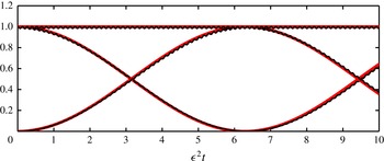
Thus the horizontally averaged kinetic energy of the balanced flow lowers the frequency of the NIWs from the initial inertial frequency, making them subinertial. Since different baroclinic modes have different $Bu$ , this can lead to vertical dispersion of the modes in SDR in the long-time limit. We compare this asymptotic prediction by numerically integrating (3.1) with $Bu=1$ and $\unicode[STIX]{x1D716}=0.125$ (since in SDR, we will need to numerically integrate for times of order $t\sim 1/\unicode[STIX]{x1D716}^{2}$ , we chose the higher Rossby number). Figure 7 shows comparisons between the asymptotic prediction and numerical solution of RSW and it is seen that the difference is negligible for the time scales considered.

Figure 7.

Comparison between asymptotic prediction for SDR (3.42) (red curve) and numerical solution of RSW (3.1) (black curve) for $\unicode[STIX]{x1D716}=0.125$ and $Bu=1$ . The straight line is $\langle u\rangle ^{2}+\langle v\rangle ^{2}$ , the curve beginning at 1 is $\langle u\rangle ^{2}$ and the curve beginning at 0 is $\langle v\rangle ^{2}$ . Observe that the black curves lie over the red curves indicating the exceptional agreement between the asymptotic predictions and numerical results.

A note on the ‘strong dispersion approximation’ of YBJ

Section 5 of YBJ introduces a further approximation to their amplitude equation based on a spatial scale separation between NIWs  and the background flow. Defining $\unicode[STIX]{x1D707}$ as the ratio of eddy horizontal scales to wave horizontal scales (equation (5.2) in YBJ), they refer to the limit $\unicode[STIX]{x1D707}\ll 1$ as the ‘strong dispersion approximation’ (SDA). Further, since SDA uses only the YBJ equation, ignoring the $O(\unicode[STIX]{x1D716})$ corrections to the leading-order wave field (expressed in equation (2.25) in YBJ), one requires $\unicode[STIX]{x1D707}\gg \unicode[STIX]{x1D716}$ and therefore one has the ordering of small parameters: $\unicode[STIX]{x1D716}\ll \unicode[STIX]{x1D707}\ll 1$ . The asymptotic expansion of the velocity field for example may be rewritten as $\mathscr{U}=A_{00}(t)+\unicode[STIX]{x1D707}A_{01}(x,y,t)+O(\text{max}(\unicode[STIX]{x1D707}^{2},\unicode[STIX]{x1D716}))$ , where $A_{00}$ and $A_{01}$ are asymptotic expansions of the leading-order NIWs amplitude $A_{0}$ , as seen in (3.10a,b ) (these are expressed as $\overline{A}$ and $A^{\prime }$ , respectively, in YBJ – see their equation (5.6)). Asymptotic expansions in $\unicode[STIX]{x1D707}$ may be used to obtain expressions for $A_{01}$ (equation (5.12) in YBJ), which is the leading-order spatially inhomogeneous wave field (since $A_{00}$ is spatially homogeneous). YBJ use this result to argue that NIWs in the SDA must concentrate in anticyclones.

In contrast the leading-order wave field in SDR is homogeneous with infinite horizontal scales, implying that $\unicode[STIX]{x1D707}\rightarrow \infty$ , and the next-order inhomogeneities are $O(\unicode[STIX]{x1D716})$ with spatial scales of the order of the mean flow scales. These $O(\unicode[STIX]{x1D716})$ inhomogeneous fields consist of pure inertial oscillations and gravity waves of varying frequencies, as indicated in (3.33a ). Since the leading inhomogeneous field in SDA is different from that in SDR, the predictions of anticyclonic trapping using the YBJ equation do not apply in SDR. This is in spite of the fact that both SDA and SDR predict the same equation for the leading-order homogeneous wave field: the SDR amplitude equation, (3.41) is identical to the SDA leading-order amplitude equation for $A_{00}$ (equation (5.10) in YBJ), despite that the procedure followed in deriving them are completely different.

Figure 8.

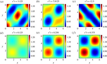
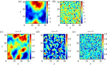
(a–c) and (d–f) show $|A|$ from the RSW and YBJ simulations, respectively. Both simulations used $Bu=1$ and $\unicode[STIX]{x1D716}=0.125$ . The solution of RSW in SDR fluctuates on a fast time scale due to the excitation of non-inertial gravity waves, as expressed in (3.33a ). The RSW solution is in general therefore very different from what may be obtained by integrating the YBJ in SDR, or based on the strong dispersion approximation on the YBJ equation, the latter being a subset of the solution of the YBJ equation. A noticeable difference is the trapping of waves in anticyclones in the YBJ case (as predicted), a feature that is not seen in the parent model, RSW even after long times.

Therefore in SDR there is no affinity of NIWs towards anticyclones, while SDA predicts the opposite. Note that since SDA uses the YBJ equation as its parent model, the solution of the YBJ equation captures all the asymptotic results obtained with $\unicode[STIX]{x1D707}$ as the small parameter. To illustrate that SDA is not valid in SDR, we integrate RSW and the YBJ equation by setting $Bu=1$ in both models; the results are shown in figure 8. The RSW solution consists of fast wave fields consisting of gravity waves and inertial waves (see (3.33)) in addition to spatially homogeneous inertial waves and, even after long times, shows no affinity towards anticyclones. In contrast, the YBJ equation integrated with the same parameters shows a tendency for the wave field to concentrate in anticyclones. This experiment indicates that the YBJ equation cannot capture the features of the SDR; therefore SDA, which is a further reduction of the YBJ equation, does not hold in the SDR.

4 Conservation laws, trapping of NIWs in anticyclones and small-scale formation in the weak dispersion regimes

In this section, we identify conservation laws for the weak dispersion amplitude equations, and in this context consider the trapping of NIWs in anticyclones and scaling arguments for breakdown of the amplitude equations in vWDR. We first note that the YBJ equation has two conservation laws (Danioux, Vanneste & Bühler Reference Danioux, Vanneste and Bühler2015, hereafter DVB). The first is

(4.1) $$\begin{eqnarray}\frac{\text{d}}{\text{d}t}\langle |A|^{2}\rangle =0,\end{eqnarray}$$

where angle brackets denote spatial averaging; it follows from $\langle \!A^{\ast }$ (3.12)  $+\,\text{c.c.}\!\rangle$ (where the $0$ subscript has been dropped). This conservation law is due to the symmetry associated with translational invariance of the phase of NIWs, i.e. $A\rightarrow A\text{e}^{\text{i}s}$ , and therefore may be called the ‘action’ integral (Xie & Vanneste Reference Xie and Vanneste2015). Note that action is also proportional to the kinetic energy of the waves ( $|A|^{2}=u^{2}+v^{2}$ ) and therefore NIWs cannot exchange kinetic energy with the mean flow. The second invariant is

(4.2a,b ) $$\begin{eqnarray}\displaystyle \frac{\text{d}}{\text{d}t}\mathscr{E}_{ybj}=0,\quad \mathscr{E}_{ybj}=E_{adv}+E_{disp}+E_{refr}, & & \displaystyle\end{eqnarray}$$

(4.3a-c ) $$\begin{eqnarray}\displaystyle E_{adv}=\text{i}\unicode[STIX]{x1D716}\left\langle \unicode[STIX]{x1D6F9}J(A^{\ast },A)\right\rangle ,\quad E_{disp}=\frac{Bu}{2}\left\langle |\unicode[STIX]{x1D735}A|^{2}\right\rangle ,\quad E_{refr}=\frac{\unicode[STIX]{x1D716}}{2}\left\langle (\unicode[STIX]{x0394}\unicode[STIX]{x1D6F9})|A|^{2}\right\rangle .\quad & & \displaystyle\end{eqnarray}$$

This follows from computing $\langle \!\text{i}\unicode[STIX]{x2202}A^{\ast }\!\,/\unicode[STIX]{x2202}t$  (3.12)  $+\,\text{c.c.}\!\rangle$ , and arises due to the time translational symmetry (consistent with the requirement of a steady mean flow) and thus may be interpreted as the ‘energy’ (however, note that this is not the physical energy – kinetic, potential or sum – of the waves). While a steady mean flow is required to obtain this conservation law, the asymptotic derivation of the amplitude equation may be extended for the case of a mean flow that evolves on the slow time scale, $\unicode[STIX]{x1D716}t$ .

It then follows that the potential energy of the wave field (proportional to $|\unicode[STIX]{x1D735}A|^{2}$ ) is not conserved, unlike kinetic energy, and thus may be exchanged with the mean flow. As was pointed out by Xie & Vanneste (Reference Xie and Vanneste2015), this is a mechanism by which the waves can extract energy from the mean flow: modulation of the waves by the mean flow leads to smaller wave scales, and hence an increase in the potential energy of the waves, potentially providing a sink for the energy of mesoscale eddies. Although Xie & Vanneste (Reference Xie and Vanneste2015) considered a parameter regime where the waves are stronger than the mean flow, due to the absence of resonant nonlinear terms, the wave evolution equation is exactly same as the basic YBJ equation (lack of nonlinear wave interaction terms for NIWs  is due to the absence of resonant wave triads or quartics between pure inertial frequency components, see for example Wagner & Young Reference Wagner and Young2016 and Zeitlin, Reznik & Ben Jelloul Reference Zeitlin, Reznik and Ben Jelloul2003). In the regime studied here, where the waves are weaker than the mean flow, the same mechanism is at play, but the energy extracted by the waves from the mean flow is asymptotically smaller than the total mean flow energy. This is also why the assumption of a steady mean flow is consistent in this study.

The IDR and vWDR equations have similar conservation laws and can be derived following the same procedure above. The first conservation law, action, remains the same for IDR and vWDR equations. The ‘energy’ conservation laws for IDR and vWDR equations are, respectively,

(4.4a-c ) $$\begin{eqnarray}\frac{\text{d}}{\text{d}t}\mathscr{E}_{idr}=0,\quad \mathscr{E}_{idr}=\mathscr{E}_{ybj}+E_{disp2},\quad E_{disp2}=-\frac{Bu^{2}}{8}\left\langle |\unicode[STIX]{x0394}A|^{2}\right\rangle\end{eqnarray}$$

and

(4.5a-c ) $$\begin{eqnarray}\frac{\text{d}}{\text{d}t}\mathscr{E}_{vwdr}=0,\quad \mathscr{E}_{vwdr}=\mathscr{E}_{ybj}+E_{refr2},\quad E_{refr2}=-\frac{\unicode[STIX]{x1D716}^{2}}{8}\left\langle |\unicode[STIX]{x0394}^{\bot }\unicode[STIX]{x1D6F9}|^{2}|A|^{2}\right\rangle .\end{eqnarray}$$

Following DVB, one may use scaling arguments applied to these conservation laws to understand why wave activity increases in anticyclones. Because the IDR and vWDR equations are basically the YBJ equation with correction terms that matter at long times, these arguments are a trivial extension of DVB and are not repeated here.

Figure 9.

(a) Streamfunction and (b) associated vorticity. (c–e) Amplitude modulus $|A|$ obtained from numerical solutions of RSW: (c) IDR ( $\unicode[STIX]{x1D716}=0.0125$ and $Bu=\sqrt{\unicode[STIX]{x1D716}}$ ); (d) YBJ ( $\unicode[STIX]{x1D716}=Bu=0.0125$ ); (e) vWDR ( $\unicode[STIX]{x1D716}=0.125$ and $Bu=\unicode[STIX]{x1D716}^{2}$ ).

We instead consider these conservation terms in the context of additional numerical simulations. For completeness we use a somewhat more natural mean flow field, obtained by numerically integrating the two-dimensional vorticity equation initialized with uniformly distributed random numbers in the interval $(0,10)$ on the grid points. The size of the domain was increased to $[0,~10\unicode[STIX]{x03C0}]\times [0,~10\unicode[STIX]{x03C0}]$ and the time integration was stopped when the vortical fields that formed had spatial scales approximately one-tenth of the domain size, so that in non-dimensional form the vortical structures of the mean flow have $O(1)$ length scales. We further scaled the r.m.s. vorticity such that $\langle (\unicode[STIX]{x0394}\unicode[STIX]{x1D6F9})^{2}\rangle =1$ . The vorticity field and the corresponding streamfunction are shown in figure 9(a,b).

Figure 9(c–e) shows the amplitude modulus $|A|$ in three cases: IDR ( $\unicode[STIX]{x1D716}=0.0125$ , $Bu=\sqrt{\unicode[STIX]{x1D716}}$ ), YBJ ( $\unicode[STIX]{x1D716}=Bu=0.0125$ ) and vWDR ( $\unicode[STIX]{x1D716}=0.125$ , $Bu=\unicode[STIX]{x1D716}^{2}$ ), by integrating the RSW equations using this non-evolving mean flow, and initialized with a homogeneous wave field. Just as in the previous section, the solutions of each amplitude equation provide faithful approximations to the RSW solutions (figures not shown, but see figure 10), although we found that in the very weak dispersion regime, on longer time scales, the solution of the vWDR amplitude equation deviates from the RSW solution due to the formation of smaller spatial scales (discussed below).

Figure 10.

Components of the energy terms in the conservation laws for the amplitude equations (4.4) for IDR (a,b), (4.2) for YBJ (c,d) and (4.5) for vWDR (e,f). (a,c,e) Show results from the respective amplitude equations, and (b,d,f) show the same terms computed from the RSW solution. In (a,b) for IDR, the curves are $E_{adv}$ (black curve), $E_{disp}$ (blue curve), $E_{refr}$ (red curve), $E_{disp2}$ (magenta curve) and $\mathscr{E}_{idr}$ (discontinuous black curve), as functions of the slow time $\unicode[STIX]{x1D716}t$ , for $\unicode[STIX]{x1D716}=0.0125$ and $Bu=\sqrt{\unicode[STIX]{x1D716}}$ . In (c,d) for YBJ, the curves are $E_{adv}$ (black curve), $E_{disp}$ (blue curve), $E_{refr}$ (red curve) and $\mathscr{E}_{ybj}$ (discontinuous black curve), as functions of the slow time $\unicode[STIX]{x1D716}t$ for $\unicode[STIX]{x1D716}=Bu=0.0125$ . In (e,f) for vWDR, the curves are $E_{adv}$ (black curve), $E_{disp}$ (blue curve), $E_{refr}$ (red curve), $E_{refr2}$ (magenta curve) and $\mathscr{E}_{vwdr}$ (discontinuous black curve), as functions of the slow time $\unicode[STIX]{x1D716}t$ for $\unicode[STIX]{x1D716}=0.125$ and $Bu=\unicode[STIX]{x1D716}^{2}$ .

Figure 10 shows time series of the energy terms in (4.2)–(4.5). Overall, the energy terms from the amplitude equations and RSW are strikingly similar. A variable that measures the correlation between anticyclonic vorticity and wave strength is $E_{refr}$ in (4.2); note that it is negative in all cases, consistent with anticyclonic trapping in the limit $Bu\ll 1$ . Figure 10(a,b) shows results from the IDR. One can see that the refraction term balances the lower-order dispersion terms. Assuming the spatial scale of waves to be $l$ , we note that $l\gg 1$ and $l\ll 1$ means the wave field has larger or smaller spatial scales than the mean flow, respectively, since the mean flow has $O(1)$ spatial scales in non-dimensional form. If we equate the refraction and dispersion terms, we obtain $l\sim \sqrt{Bu/\unicode[STIX]{x1D716}}\gg 1$ as a scaling estimate for the wave field, implying that the spatial scale of the wave field is larger than that of the mean flow in this regime, as also seen in figure 9(c).

In the vWDR experiment shown in figure 10(e,f), one sees that the total energy $\mathscr{E}_{vwdr}$ , although exactly conserved in the amplitude equation, increases with time when calculated using the RSW solution, indicating a breakdown of the assumptions that led to the vWDR amplitude equation. Note that both of the refraction terms are negligible (consistent with results shown in § 3), with instead the advection term balancing the dispersion term. This is a consequence of the small spatial scale formation in the wave field, resulting in amplification of the spatial derivatives of the wave amplitude. These two features are also obvious from figure 9(e).

To understand this, consider the following scaling argument. Balancing the dispersive and advection terms, we find $l\sim Bu/\unicode[STIX]{x1D716}$ and since $Bu\sim \unicode[STIX]{x1D716}^{2}$ we obtain an estimate for the scales of the wave field as $l\sim \unicode[STIX]{x1D716}$ . Since the horizontal length of the wave field scales as $l\sim \unicode[STIX]{x1D716}$ the advective nonlinearity $U/fl$ , which resembles Rossby number with wavelength scale $l$ replacing mean flow scale $L$ , can reach $O(1)$ values and pressure gradients can increase beyond the scaling assumptions of vWDR. We plot the pressure gradient terms and the largest mean flow interaction terms in figure 11. Observe that the mean flow interaction terms become $O(1)$ , invalidating our asymptotic analysis which assumed these terms to be small. Similarly, the pressure gradient term becomes $O(\unicode[STIX]{x1D716})$ , since $Bu\unicode[STIX]{x1D735}p\sim \unicode[STIX]{x1D716}^{2}/l\sim \unicode[STIX]{x1D716}$ , violating the initial scaling of $O(\unicode[STIX]{x1D716}^{2})$ . However, we note that the wave field is still near inertial, since the pressure gradient term is asymptotically small. The breakdown of the asymptotic model due to the increased magnitude of the mean flow interaction terms imply that the conservation law for the vWDR amplitude equation need not be conserved when calculated using RSW.

We observe that the refraction term is negative definite in IDR and takes very small negative values in vWDR. This term is therefore expected to be negative in the regime $Bu\sim \unicode[STIX]{x1D716}$ , assuming a smooth change in variables. This is the crux of the argument made in DVB to explain trapping of waves in anticyclones based on the YBJ equation. Further, while IDR and vWDR have, respectively, larger and smaller spatial scales than the mean flow, the $Bu\sim \unicode[STIX]{x1D716}$ regime has scales comparable to that of the mean flow, as can be seen in figure 9(d). As a consequence, dispersion, refraction and advection terms in the amplitude equation are all non-negligible, as may be inferred from figure 10(c,d), a feature that is faithfully observed in RSW as well.

Figure 11.

$Bu\sqrt{\langle |\unicode[STIX]{x1D735}p|^{2}\rangle }$ (red curve) and $\unicode[STIX]{x1D716}\sqrt{\langle |\boldsymbol{V}\boldsymbol{\cdot }\unicode[STIX]{x1D735}p|^{2}\rangle }$ (black curve) obtained by integrating RSW with the same parameters used for figure 10(e,f).

In summary, we note three important observations resulting from this section. Scaling arguments applied to the conservation laws, as pointed out by DVB, can be easily modified for the IDR and vWDR equations and therefore the increased wave activity in anticyclones is a generic feature of the weak dispersion regime. Further, energy components when calculated using RSW solutions agree quite well with the amplitude equation predictions, which again is not an obvious statement for an arbitrary mean flow such as the one we considered. Finally, based on scaling estimates, we find that the vWDR develops small-scale features as a generic property, resulting in $O(1)$ advective nonlinearity, $U/fl$ , for the wave field. This restricts the long-term validity of a reduced model in this regime.