1 Introduction
Laboratory investigations are paramount to understanding the fundamental magnetic energy to plasma kinetic energy conversion mechanism of magnetic reconnection. Full descriptions of reconnection phenomena observed in both astrophysical environments, e.g. active galactic nuclei (Nalewajko Reference Nalewajko2016), solar flares (Karlický Reference Karlický2014), planetary magnetospheres (Fuselier et al. Reference Fuselier, Lewis, Schiff, Ergun, Burch, Petrinec and Trattner2016) and experimental magnetic islands, e.g. within fusion reactors (Grasso et al. Reference Grasso, Margheriti, Porcelli and Tebaldi2006, Reference Grasso, Lazzaro, Borgogno and Comisso2016), depend on our intimate understanding of three-dimensional (3-D) reconnection processes. Numerous laboratory experiments have been undertaken that attempt to reproduce the observed topological signatures seen in these dynamic plasma environments, e.g. current sheet-3D (CS-3D; Frank et al. Reference Frank, Bogdanov, Markov, Ostrovskaya and Dreiden2005), Tokyo Spheromak (TS-3/4; Ono et al. Reference Ono, Morita, Katsurai and Yamada1993), Magnetic Reconnection Experiment (MRX; Yamada et al. Reference Yamada, Ji, Hsu, Carter, Kulsrud, Bretz, Jobes, Ono and Perkins1997a ), Facility for Laboratory Reconnection Experiments (FLARE; Ji et al. Reference Ji, Yamada, Hsu and Kulsrud1998, Reference Ji, Bhattacharjee, Prager, Daughton, Bale, Carter, Crocker, Drake, Egedal and Sarff2014), Swarthmore Spheromak Experiment (SSX; Brown, Cothran & Fung Reference Brown, Cothran and Fung2006), Versatile Toroidal Facility (VTF; Egedal et al. Reference Egedal, Fasoli, Porkolab and Tarkowski2000, Reference Egedal, Fasoli, Tarkowski and Scarabosio2001), and 3D Electron Magnetohydrodynamics (EMHD; Stenzel et al. Reference Stenzel, Urrutia, Griskey and Strohmaier2001, Reference Stenzel, Urrutia, Griskey and Strohmaier2002).
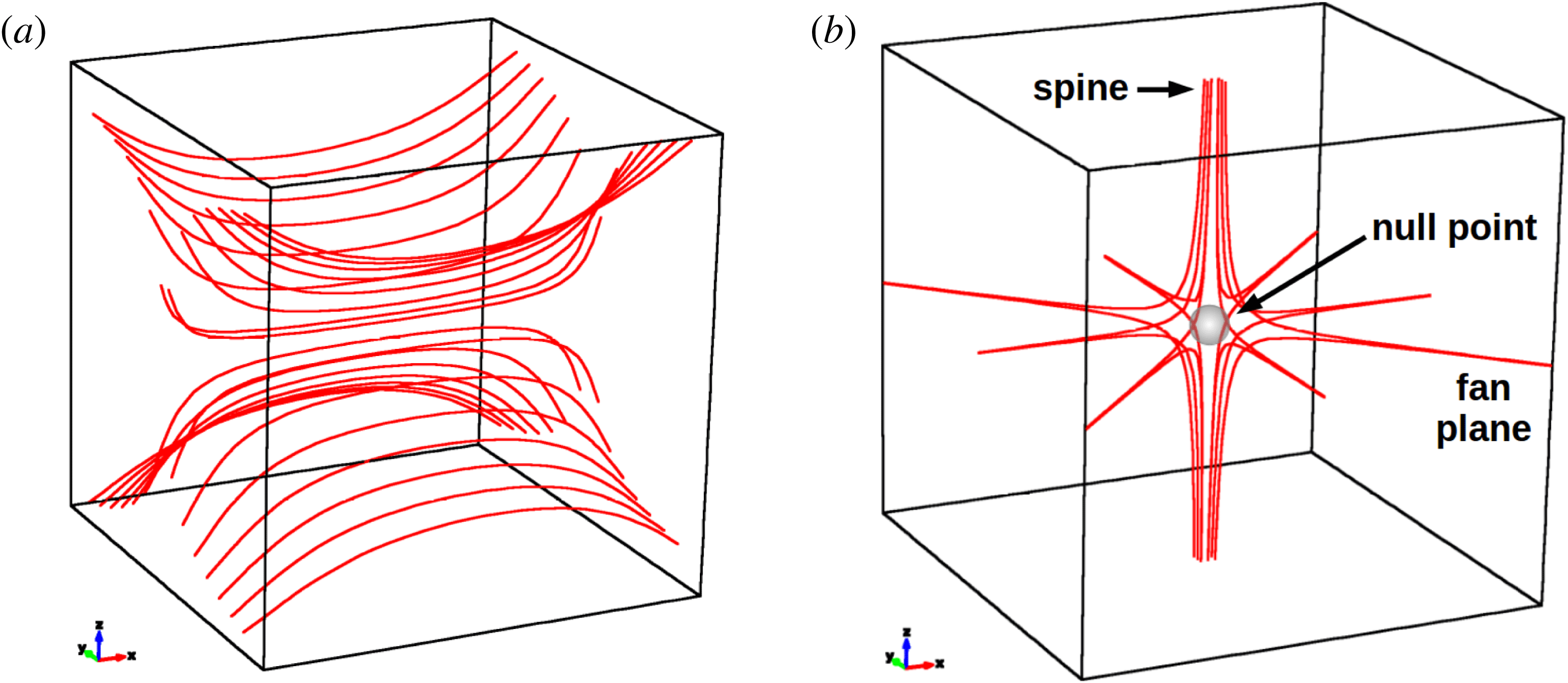
Most of these spheromak and tokamak-style experiments have been designed for and primarily focused on inducing quasi-axisymmetric ‘X-line’ reconnecting plasma current sheets (figure 1 a) featuring ‘double Y’ or ‘O’ shaped diffusion regions of Sweet–Parker, Petschek-style reconnection (Biskamp Reference Biskamp1986; Yamada et al. Reference Yamada, Ji, Hsu, Carter, Kulsrud, Ono and Perkins1997b ; Ji et al. Reference Ji, Yamada, Hsu and Kulsrud1998). While these operational experiments represent a significant step forward in our understanding of X-line reconnection processes (Yamada et al. Reference Yamada, Ji, Hsu, Carter, Kulsrud, Ono and Perkins1997b ; Ji et al. Reference Ji, Yamada, Hsu and Kulsrud1998; Egedal et al. Reference Egedal, Fox, Katz, Porkolab, Reim and Zhang2007; Yamada et al. Reference Yamada, Yoo, Jara-Almonte, Ji, Kulsrud and Myers2014), only EMHD at UCLA (Stenzel et al. Reference Stenzel, Urrutia, Griskey and Strohmaier2001, Reference Stenzel, Urrutia, Griskey and Strohmaier2002) has been designed to study the fan spine topology about isolated null points (figure 1 b) (Parnell et al. Reference Parnell, Smith, Neukirch and Priest1996), to our knowledge. As 3-D null points are known to be ubiquitous in astrophysical environments such as the solar atmosphere (Longcope & Parnell Reference Longcope and Parnell2009; Pontin, Priest & Galsgaard Reference Pontin, Priest and Galsgaard2013; Edwards & Parnell Reference Edwards and Parnell2015; Freed, Longcope & McKenzie Reference Freed, Longcope and McKenzie2015) and in laboratory plasma environments of mixed magnetic polarity (Grasso et al. Reference Grasso, Margheriti, Porcelli and Tebaldi2006, Reference Grasso, Lazzaro, Borgogno and Comisso2016), a deeper understanding of reconnection manifesting as field line slippages near an isolated magnetic null point is required.
(a) Topological structure of magnetic field lines in Sweet–Parker, Petscjek-style spheromak and tokamak reconnection (Yamada et al. Reference Yamada, Ji, Hsu, Carter, Kulsrud, Ono and Perkins1997b ). (b) Topological structure of three-dimensional magnetic field lines about an isolated magnetic null point with the two-dimensional fan plane and the antiparallel spine axis (Pontin Reference Pontin2012). Torsional spine reconnection (TSR) is characterized by fan field line slippages and current sheet amplification concentrated along the spine axis.

In the laboratory set-up of EMHD (Stenzel et al.
Reference Stenzel, Urrutia, Griskey and Strohmaier2001, Reference Stenzel, Urrutia, Griskey and Strohmaier2002), 3-D magnetic nulls were formed in pairs and connected by separator lines. The nulls arise from a unique initial potential magnetic field within an ambient argon plasma, and plasma and magnetic field perturbations were initiated by rapid current dissipation through a circular antenna. It was observed that the initial radial nulls were deformed into improper spiral nulls due to magnetic gradient-induced relaxation currents along the spine. However, no narrow current sheets, no anomalous resistivity and no plasma vortices on the scale of the electron inertial length
 $d_{e}=c/\unicode[STIX]{x1D714}_{pe}$
were reported (Stenzel et al.
Reference Stenzel, Urrutia, Griskey and Strohmaier2001). These noted discrepancies with both resistive magnetohydrodynamic (MHD) and kinetic magnetic reconnection led the authors to suggest further investigations of reconnection at 3-D null points are required.
While these EMHD experiments and observations represented a significant step forward in observing plasma motions in proximity to isolated 3-D magnetic nulls, no operational experiment is able to drive one of the three modes of 3-D reconnection about an isolated magnetic null point: spine fan reconnection, torsional fan reconnection or torsional spine reconnection (Priest & Pontin Reference Priest and Pontin2009). In order to explore the complete nature and origin of localized current sheet formation and current accumulation about isolated 3-D magnetic null regions, as well as to decipher the physics of reconnection-driven plasma heating and particle acceleration, experimental set-ups must be considered for studying these 3-D reconnection modes.
This paper describes the initial design of an experiment featuring driven torsional spine reconnection (TSR). The TSR mode has been successfully demonstrated by kinetic models and robust 3-D MHD simulations (Pontin & Galsgaard Reference Pontin and Galsgaard2007; Pontin, Al-Hachami & Galsgaard Reference Pontin, Al-Hachami and Galsgaard2011) and is known to occur within the diffusion regions of solar plasma jet phenomena (e.g. Pontin et al. Reference Pontin, Priest and Galsgaard2013) and planetary magnetosheaths (Wendel & Adrian Reference Wendel and Adrian2013). The magnetic field dynamics leading to TSR is based upon driven rotational perturbations in the fan plane, centred around the spine. The plasma motions and current sheet amplification resulting from field line slippages are centred around the open magnetic field lines of the null point spine axis, a feature unable to be induced in experimental X-line reconnection investigations of solar chromospheric jets (Nishizuka et al. Reference Nishizuka, Hayashi, Tanabe, Kuwahata, Kaminou, Ono, Inomoto and Shimizu2012).
Leveraging the results of previous investigations (Parnell et al. Reference Parnell, Smith, Neukirch and Priest1996, Reference Parnell, Neukirch, Smith and Priest1997; Pontin & Galsgaard Reference Pontin and Galsgaard2007; Pontin et al. Reference Pontin, Al-Hachami and Galsgaard2011), this work identifies components of existing technology that can mimic the necessary dynamics for inducing the TSR mode. Going forward, it is important to note that our goal is not to investigate a laboratory environment matching the quantitative plasma parameters of any observed astrophysical plasma (e.g. the solar corona), but to investigate the range of plasma scales and dynamic boundary conditions that are achievable in other laboratory plasmas that will allow for the qualitative magnetic field topologies of the TSR mode to be investigated.
In § 2, we identify and discuss two enabling components of existing technology that, when combined, mimic the qualitative magnetic field topologies required for the induction of TSR. In § 3, under both resistive MHD and kinetic theory constraints, we first show that the quantitative plasma parameters of these enabling components satisfy the frozen-in condition. Second, we estimate the scales on which the breakdown of the frozen-in condition is must occur. A first-order approximation to this system’s operational performance is presented in § 4 by parameterizing resistive MHD and kinetic responses to perturbations, and directly comparing results against those of the identified technologies. Finally, in § 6 we argue that examining the feasibility of such an experiment will open new capabilities for investigations of 3-D magnetic reconnection and deepen our understanding of the numerous modes of this ubiquitous astrophysical process. Magnetic reconnection is a scalable particle acceleration mechanism that occurs across the range of length scales of astrophysical plasmas. Therefore, we suggest that miniaturizing this process can be exploited for practical applications from ion beam technologies to spacecraft propulsion, the latter of which was first identified by Chesny (Reference Chesny2013) and recently expanded upon by Cazzola et al. (Reference Cazzola, Curreli, Markidis and Lapenta2016).
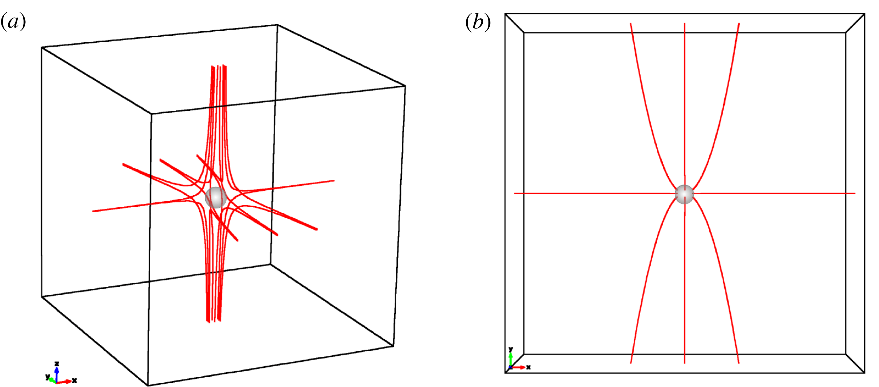
(a) Topological structure of the improper radial PNP field with
 $p=2.0$
and
 $q=j_{\Vert }=j_{\bot }=0.0$
with fan field lines concentrated along the
 $y$
-axis, the major axis of the null. This is the form of the potential magnetic field that is perturbed to induce TSR in robust simulations (Pontin et al.
Reference Pontin, Al-Hachami and Galsgaard2011). (b) View of the
 $xy$
fan plane. Such fields can be produced via state-of-the-art conducting coil technology (Goodzeit, Meinke & Ball Reference Goodzeit, Meinke and Ball2005).

2 A candidate TSR system
At the most basic level, reconnection experiments can be described by a two-step process. First, the system is set-up with plasma frozen into a static (potential) magnetic field with cusp or null regions where
 $\boldsymbol{B}=0$
. Second, an externally driven instability is introduced that forces the breakdown of the frozen-in condition, allowing current sheets to form and reconnection to occur (Yamada et al.
Reference Yamada, Ji, Hsu, Carter, Kulsrud, Bretz, Jobes, Ono and Perkins1997a
; Egedal et al.
Reference Egedal, Fasoli, Porkolab and Tarkowski2000). Robust simulations of the TSR mode (Pontin & Galsgaard Reference Pontin and Galsgaard2007; Pontin et al.
Reference Pontin, Al-Hachami and Galsgaard2011) provide an infrastructure in which to identify existing technologies that can mimic such behaviour.
The driven reconnection mode of TSR first requires an isolated potential 3-D null point field following the
 $\boldsymbol{B}=\boldsymbol{M}\boldsymbol{\cdot }\boldsymbol{r}$
matrix formulation of Parnell et al. (Reference Parnell, Smith, Neukirch and Priest1996), where
 $\boldsymbol{B}$
is the magnetic field,
 $\boldsymbol{M}$
is a
 $3\times 3$
magnetization tensor, and
 $\boldsymbol{r}$
is the 3-D position vector. The potential field parametrization of Pontin et al. (Reference Pontin, Al-Hachami and Galsgaard2011) using
 $p=2$
and
 $q=j_{\Vert }=j_{\bot }=0$
produced an improper radial null point field, identical to that shown in figure 2, with fan field lines concentrated along the
 $y$
-axis of the null. It is important to note that the parameters
 $p$
and
 $q$
describe the potential part of the null point magnetic field, and
 $j_{\Vert }$
and
 $j_{\bot }$
affect the twist and inclination of the fan plane, respectively. Both spheromak and tokamak-style technologies for X-line experiments (e.g. Yamada et al.
Reference Yamada, Ji, Hsu, Carter, Kulsrud, Bretz, Jobes, Ono and Perkins1997a
, Egedal et al.
Reference Egedal, Fasoli, Tarkowski and Scarabosio2001) and 3-D EMHD (Stenzel et al.
Reference Stenzel, Urrutia, Griskey and Strohmaier2001) used multiple relatively large (
 ${\sim}70~\text{cm}$
diameter) flux cores for the production of their potential fields. Such conditions were required for their large system sizes
 $L$
to satisfy the conditions of MHD plasma (see § 3). Fortunately, state-of-the-art multi-layer helical conducting coil technology (e.g. Meinke, Senti & Stelzer Reference Meinke, Senti and Stelzer1997, Goodzeit et al.
Reference Goodzeit, Meinke and Ball2005) can be optimized to produce unique null point fields of high purity (such as figure 2), and machined to fit within a volume of
 ${\lesssim}1~\text{m}^{3}$
. The use of such concentric multi-layer coils have wide ranging applications for high-order multipole fields in particle accelerator beam steering applications and MHD thrust devices. While smaller volumes reduce the global scale length
 $L$
parameter space within which ideal MHD conditions may prevail, the described TSR experiment is designed to overcome this shortcoming with the use of a dense plasma and still satisfy the frozen-in condition (see below and § 3). This is possible since magnetic reconnection is fundamentally a multi-scaled self similar process (Chang Reference Chang1999; Raouafi et al.
Reference Raouafi, Georgoulis, Rust and Bernasconi2010; Chesny et al.
Reference Chesny, Oluseyi, Orange and Champey2015; Chesny, Oluseyi & Orange Reference Chesny, Oluseyi and Orange2016; Wyper, Antiochos & DeVore Reference Wyper, Antiochos and DeVore2017).
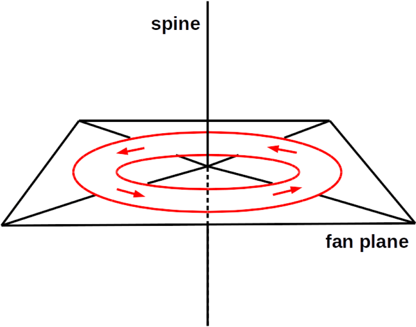
In the TSR simulations of Pontin & Galsgaard Reference Pontin and Galsgaard2007 and Pontin et al. Reference Pontin, Al-Hachami and Galsgaard2011, a rotational magnetic field perturbation to the field lines of the fan plane, centred around the spine axis (figure 3), caused the propagation of Alfvén waves toward and away from the null. The TSR mode of interest to this work occurs due to the ingoing wave as it propagates along the background magnetic field lines to form a concentric cylindrical current tube centred around the spine. The bulk plasma flow is rotational, with the peak spine-directed current increasing as the wave localizes around the vicinity of the spine. This collapsed wavefront induces the rotational slippage of the perturbed field lines and is observed as a current intensification close to the spine. This helical Alfvén wave (Galsgaard, Priest & Titov Reference Galsgaard, Priest and Titov2003) is dominated by the current component oriented parallel to the spine. The bulk rotational plasma flows associated with TSR peak as field line diffusion maximizes, and then reverse direction once the rotational slippages relax back to their low-energy potential state.
Fan spine magnetic null point topology (black vectors) with applied circular magnetic field perturbation (red vectors). This configuration was shown to lead to TSR (Pontin & Galsgaard Reference Pontin and Galsgaard2007; Pontin et al. Reference Pontin, Al-Hachami and Galsgaard2011). Hardware that can mimic these magnetic field dynamics may open up the possibility for a laboratory set-up that can induce TSR.

To design an experiment for inducing TSR featuring these observational signatures, an apparatus placed in the conducting coil-produced potential null point field must provide a circular magnetic field perturbation to the fan plane, centred around the spine. A dense plasma focus (DPF) is a cylindrical apparatus that produces a dense (Guillory, Rose & Lerner Reference Guillory, Rose, Lerner, Kusse and Hammer2009; Mitrofanov et al.
Reference Mitrofanov, Krauz, Kubes, Scholz, Paduch and Zielinska2014; Huba Reference Huba2016) (
 ${\sim}10^{24}~\text{m}^{-3}$
) MHD-scale (Caballero Bendixsen et al.
Reference Caballero Bendixsen, Bott-Suzuki, Cordaro, Krishnan, Chapman, Coleman and Chittenden2016) capacitively coupled plasma featuring an azimuthal magnetic field within its toroidal plasma sheath (Lindberg & Jacobsen Reference Lindberg and Jacobsen1961; Guillory et al.
Reference Guillory, Rose, Lerner, Kusse and Hammer2009; Krishnan & Thompson Reference Krishnan and Thompson2010). Most DPFs are a few centimetres in both length and in radius and are small enough to be able to be operated inside the inner volume of a conducting coil of
 ${\lesssim}1~\text{m}^{3}$
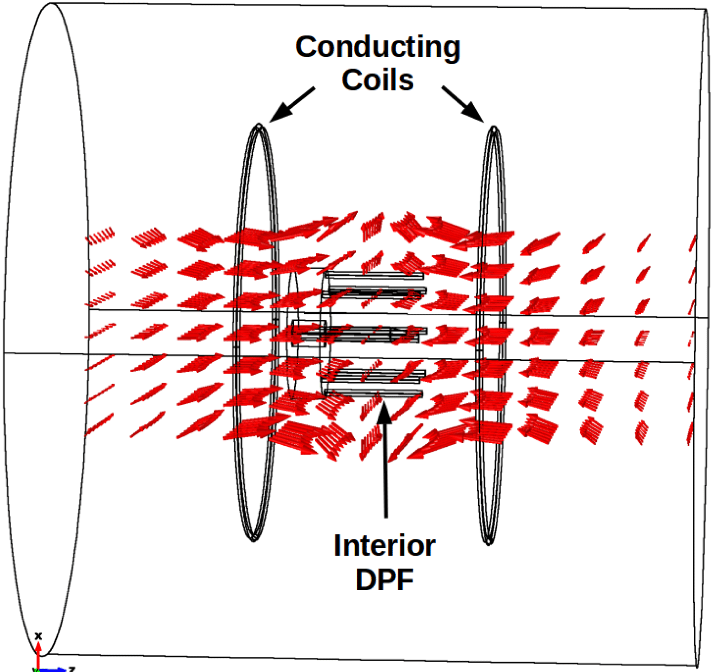
. It is feasible that a dedicated experiment comprised of a conducting coil null point field and a central DPF, having the coil’s central spine axis aligned with the DPF axial direction (figure 4), could mimic the TSR magnetic field dynamics of figure 3.
Generalized COMSOL Multiphysics model geometry of DPF (interior black contours) immersed in null point field (red vectors) produced by two conducting loops carrying equal current in opposite directions. The operation of the DPF apparatus within this field is the principle of operation. The optimized apparatus is anticipated to fit within
 ${\lesssim}1~\text{m}^{3}$
.

We have calculated magnetic field solutions for both the theoretical topology leading to TSR (Pontin et al. Reference Pontin, Al-Hachami and Galsgaard2011) and the described laboratory TSR system. The theoretical magnetic null point field is characterized by (Parnell et al. Reference Parnell, Smith, Neukirch and Priest1996),
 $$\begin{eqnarray}\boldsymbol{B}=B_{0}[x+{\textstyle \frac{1}{2}}(q-j_{\Vert })y,{\textstyle \frac{1}{2}}(q+j_{\Vert })x+py,j_{\bot }y-(p+1)z].\end{eqnarray}$$
The circular magnetic field perturbation used by Pontin et al. (Reference Pontin, Al-Hachami and Galsgaard2011) is a polar coordinate field in the fan plane of the form,
 $$\begin{eqnarray}B_{\unicode[STIX]{x1D703}}=B_{p}\exp \left[-\left(\frac{r-r_{0}}{a}\right)^{2}-\left(\frac{z-z_{0}}{b}\right)^{2}\right].\end{eqnarray}$$
A purely radial null with
 $p=1$
,
 $q=j_{\Vert }=j_{\bot }=0$
and
 $B_{0}=3~\text{T}$
will produce a magnetic field of the order of
 $10^{-1}~\text{T}$
approximately
 ${\sim}3~\text{cm}$
from the null region. A circular perturbation with
 $r_{0}=0.02~\text{m}$
,
 $a=0.01~\text{m}$
and
 $B_{p}=12~\text{T}$
, corresponding to centimetre-scale geometries, will produce a ring of flux of the order of
 $10^{-1}~\text{T}$
at a radial distance of
 $2~\text{cm}$
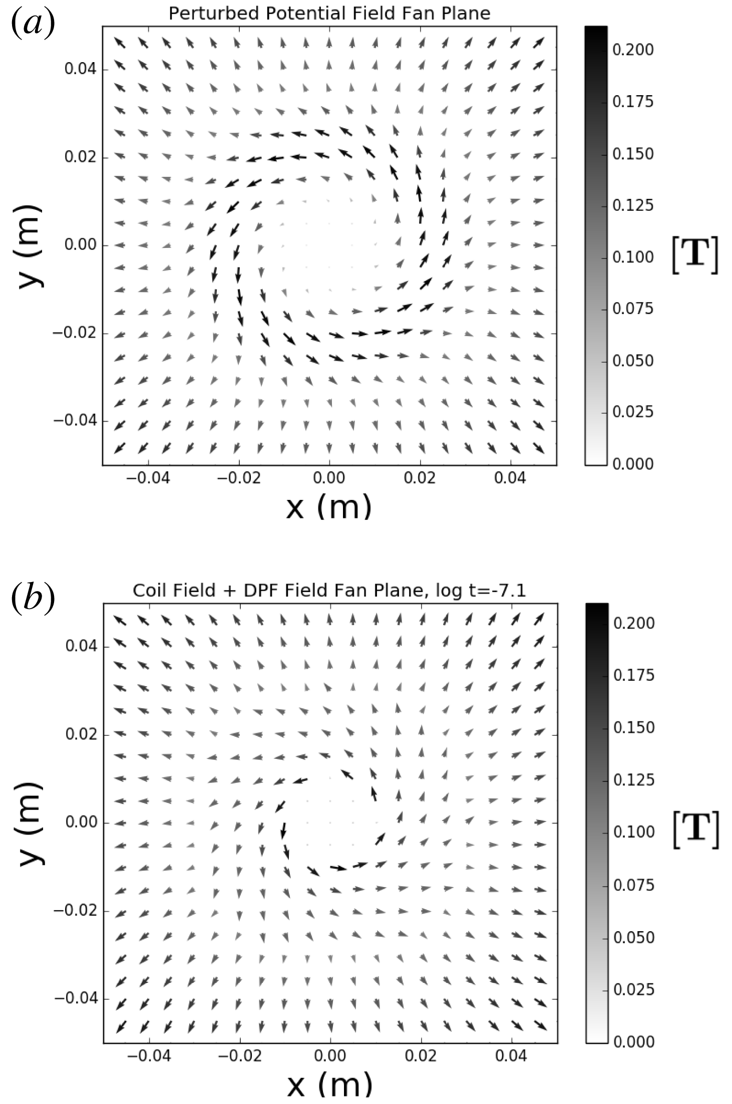
from the null. These combined fields are shown in figure 5(a) and depict the dynamics in figure 3.
For the coil–DPF system, a first-order approximation to a radial magnetic null point field was produced by solving the Biot–Savart law for two axially aligned, circular current carrying loops of radius 10 cm, offset from one another by 20 cm (figure 4). To produce a central positive null point similar to (2.1) and figure 5(a), each loop will have oppositely running current of magnitude 100 kA. This ensures a magnetic field strength of
 ${\sim}10^{-1}~\text{T}$
close to the null (see § 2). These first-order currents are obviously high, but can be mitigated to
 ${\lesssim}10^{2}$
. A using multi-layered helical conducting coil technology that produce fields of
 ${\gtrsim}1~\text{T}$
(Meinke et al.
Reference Meinke, Senti and Stelzer1997; Goodzeit et al.
Reference Goodzeit, Meinke and Ball2005). The initial magnetic curl of a DPF, leading to the formation of a flat-top toroidal plasma sheath, is created via a rapidly changing electric flux across coaxial conductors. We have solved for a general DPF field using the Ampère–Maxwell relation
 $\int \boldsymbol{B}\boldsymbol{\cdot }\text{d}\boldsymbol{l}=\unicode[STIX]{x1D707}_{0}\unicode[STIX]{x1D716}_{0}(\text{d}/\text{d}t)\oint \boldsymbol{E}\boldsymbol{\cdot }\text{d}\boldsymbol{a}$
and a discharging capacitor bank
 $Q(t)=CV\text{e}^{-t/RC}$
as,
 $$\begin{eqnarray}B_{\unicode[STIX]{x1D703}}(r,t)\text{[T]}=\frac{-\unicode[STIX]{x1D707}_{0}V}{2\unicode[STIX]{x03C0}Rr}\text{e}^{-t/RC},\end{eqnarray}$$
where
 $V$
is the voltage,
 $R$
is the resistance,
 $C$
is the capacitance,
 $r$
is the radial distance and
 $t$
is the time elapsed since the discharge. We have adopted the values of
 $V=30~\text{kV}$
,
 $R=1~\text{m}\unicode[STIX]{x1D6FA}$
, and
 $C=12.5~\unicode[STIX]{x03BC}\text{F}$
which are representative values for similar experiments (e.g. Heo & Park Reference Heo and Park2002, Bures et al.
Reference Bures, Krishnan, Madden and Blobner2010, El-Aragi Reference El-Aragi2010, Abdou et al.
Reference Abdou, Ismail, Mohamed, Lee, Saw and Verma2012, Bures, Krishnan & James Reference Bures, Krishnan and James2012, Caballero Bendixsen et al.
Reference Caballero Bendixsen, Bott-Suzuki, Cordaro, Krishnan, Chapman, Coleman and Chittenden2016). Time
 $t\approx 8\times 10^{-8}~\text{s}$
corresponds to an idealized capacitor bank rise time (Lerner, Krupakar Murali & Haboub Reference Lerner, Krupakar Murali and Haboub2011) with a magnetic field of
 $10^{-1}~\text{T}$
located 1 cm from the null. Figure 5(b) shows the superposition of the two-coil null point field and the azimuthal DPF perturbation field of (2.3). The similarities between the parametric and first-order hardware fields are obvious, i.e. both perturbations are able to deform the fan plane of the initial potential fields in a circular fashion. Therefore, it can be anticipated that, in the first order, a conducting coil–DPF combination can mimic the magnetic field dynamics leading to TSR (figure 3). In operational DPF systems, this magnetic curl is maintained and expanded radially toward the boundaries of the outer electrodes by the axial cascade of the toroidal plasma sheath following the snowplough model (Lindberg & Jacobsen Reference Lindberg and Jacobsen1961; Hart Reference Hart1964; Willenborg & Hendricks Reference Willenborg and Hendricks1976; Lee Reference Lee1983; Ziemer & Choueiri Reference Ziemer and Choueiri2001; Tang, Adams & Rusnak Reference Tang, Adams and Rusnak2010). The
 $\boldsymbol{J}\times \boldsymbol{B}$
force due to the interaction between the collisionally excited plasma current (Krishnan & Thompson Reference Krishnan and Thompson2010) and the magnetic curl of (2.3) induces the
 ${\sim}10~\unicode[STIX]{x03BC}\text{s}~\text{cm}^{-1}$
axial propagation of the sheath (Lee & Serban Reference Lee and Serban1996) in which the in situ flat-top plasma for reconnection resides.
(a) Theoretical parametrization of radial potential null point field (Parnell et al. Reference Parnell, Smith, Neukirch and Priest1996) with applied circular magnetic field perturbation (Pontin et al. Reference Pontin, Al-Hachami and Galsgaard2011). (b) Circular DPF field immersed in radial potential null point field produced from current carrying loops. Both fields are topologically similar to figure 3.

3 TSR parameterization
While the qualitative topologies of the conducting coil–DPF combination mimic the magnetic field dynamics that is known to induce the TSR mode, it must be demonstrated that the quantitative plasma parameters of such a system can lead to the onset of reconnection. In either astrophysical or laboratory plasma environments, reconnection occurs within thin localized regions much smaller than the global length scale (current sheets). Within these localized regions, the frozen-in flux condition is broken and non-ideal effects, such as diffusion or particle de-magnetization, can begin to dominate and force field line connectivity changes through the plasma.
Here, we consider the quantitative plasma parameters for the centimetre-scale, capacitively coupled TSR experiment described in § 2 in both collisional resistive MHD (Gonzalez & Parker Reference Gonzalez and Parker2016) and collisionless two-fluid, ion–electron kinetic contexts (Büchner Reference Büchner1999). General plasma parameters such as the electron–ion collision frequency
 $\unicode[STIX]{x1D708}_{c}$
are derived from the Naval Research Laboratory (NRL) Plasma Formulary (Huba Reference Huba2016). Calculated parameters such as electron plasma frequency
 $\unicode[STIX]{x1D714}_{pe}$
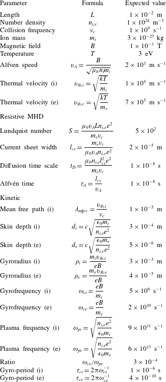
are compared to the Formulary for verification. Table 1 shows a compilation of the requisite resistive MHD and kinetic parameters along with their formulas.
Plasma parameters calculated for the investigated TSR regime.

3.1 Resistive MHD
Resistive MHD first relies on a global frozen-in flux condition of length scale
 $L$
. These ideal MHD conditions are satisfied by a large Lundquist number (
 $S\gg 1$
) of the form,
 $$\begin{eqnarray}S=\frac{v_{A}L}{\unicode[STIX]{x1D702}}=\unicode[STIX]{x1D707}_{0}\unicode[STIX]{x1D70E}v_{A}L=\frac{\unicode[STIX]{x1D707}_{0}v_{A}Ln_{e}e^{2}}{m_{e}\unicode[STIX]{x1D708}_{c}},\end{eqnarray}$$
where
 $v_{A}$
is the local Alfvén velocity,
 $L$
is the length scale of the system,
 $\unicode[STIX]{x1D702}$
is the magnetic diffusivity
 $(\unicode[STIX]{x1D707}_{0}\unicode[STIX]{x1D70E})^{-1}$
,
 $\unicode[STIX]{x1D707}_{0}$
is the vacuum permeability,
 $\unicode[STIX]{x1D70E}$
is the conductivity,
 $n_{e}$
is the electron number density,
 $e$
is the electric charge,
 $m_{e}$
is the electron mass and
 $\unicode[STIX]{x1D708}_{c}$
is the electron–ion collision frequency. Second, an abrupt change of plasma conditions results in a localized breakdown of ideal MHD (Kivelson & Russell Reference Kivelson and Russell1995; Kallenrode Reference Kallenrode2004). It is within this region where the limit
 $S\lesssim 1$
is reached that plasma diffusion across field lines is permitted and localized current sheets will form. The
 $S\sim 1$
limit of (3.1) predicts a current sheet thickness
 $l_{cs}$
of order (Kivelson & Russell Reference Kivelson and Russell1995),
 $$\begin{eqnarray}l_{cs}\sim \frac{1}{\unicode[STIX]{x1D707}_{0}\unicode[STIX]{x1D70E}v_{A}}\sim \frac{m_{e}\unicode[STIX]{x1D708}_{c}}{\unicode[STIX]{x1D707}_{0}v_{A}n_{e}e^{2}}.\end{eqnarray}$$
Though a breakdown of ideal MHD must occur within the region of current sheet formation, as required for plasma advection across field lines, outside the current layer the ideal MHD approximation should remain valid.
In the MHD portion of table 1, the initial conducting plasma state is shown by
 $S\sim 10^{2}$
. The fully resistive plasma condition (
 $S\sim 1$
) via field line diffusion is expected to occur on small spatial scales of current sheet widths of the order of
 $10^{-5}~\text{m}$
. Such effects are predicted to occur on the diffusion time scale,
 $$\begin{eqnarray}\unicode[STIX]{x1D70F}_{D}=\frac{l_{cs}^{2}}{\unicode[STIX]{x1D702}}=\unicode[STIX]{x1D707}_{0}\unicode[STIX]{x1D70E}l_{cs}^{2}=\frac{\unicode[STIX]{x1D707}_{0}n_{e}e^{2}l_{cs}^{2}}{m_{e}\unicode[STIX]{x1D708}_{c}}.\end{eqnarray}$$
The TSR
 $\unicode[STIX]{x1D70F}_{D}$
time scale of
 $10^{-8}~\text{s}$
, over which collisional instabilities dissipate, should be equivalent to a few Alfvén times
 $\unicode[STIX]{x1D70F}_{A}=l_{cs}/v_{A}$
that is a signature of 2-D X-line reconnection (Imshennik & Syrovatskiǐ Reference Imshennik and Syrovatskiǐ1967; Parnell et al.
Reference Parnell, Neukirch, Smith and Priest1997). Such behaviour will be investigated further in § 4. These values in the collisional regime now must be compared to corresponding length and time scales predicted by collisionless kinetic theory to see how they differ, and to eventually determine what effects should be expected from the TSR set-up described in § 2.
3.2 Kinetics
MHD equations characterize the behaviour of plasma and magnetic fields to a high degree (Gonzalez & Parker Reference Gonzalez and Parker2016). However, in plasma environments where currents and the Hall MHD term (
 $\boldsymbol{J}\times \boldsymbol{B}$
) become important for determining the electric field and reconnection rate, e.g. the solar corona, a two-fluid, ion–electron kinetic model may be more appropriate. In this regime, collisionless reconnection occurs when the frozen-in condition is broken on the inertial length scales of electron motion due to anomalous resistivity. Such kinetic effects have been demonstrated in plasma simulations where the TSR mode dominates (Olshevsky et al.
Reference Olshevsky, Divin, Eriksson, Markidis and Lapenta2015).
While the frozen-in condition was determined via resistive MHD equations, the breakdown must occur on inertial scales of the electron skin depth (Büchner Reference Büchner1999; Stenzel et al. Reference Stenzel, Urrutia, Griskey and Strohmaier2001),
 $$\begin{eqnarray}d_{e}=c\sqrt{\frac{\unicode[STIX]{x1D716}_{0}m_{e}}{n_{e}e^{2}}},\end{eqnarray}$$
where
 $c$
is the speed of light,
 $\unicode[STIX]{x1D716}_{0}$
is the permittivity of free space and
 $e$
is the electric charge. Table 1 shows that kinetic effects in this set-up would occur on scales an order of magnitude smaller than resistive MHD (
 $d_{e}\sim 10^{-1}l_{cs}$
).
Reconnection time scales due to kinetic effects should be a few electron gyro-periods
 $\unicode[STIX]{x1D70F}_{ce}=2\unicode[STIX]{x03C0}\unicode[STIX]{x1D714}_{ce}^{-1}$
. Bulk plasma wave perturbations propagating at the Alfvén speed heat the electrons, effectively de-magnetizing them and breaking the frozen-in condition. Unfrozen electrons are free to induce changes in magnetic connectivity, and thus reconnection. Such effects must occur within a few electron gyro-periods (see § 4) so that electron energization is not damped away (Büchner Reference Büchner1999). It is easily seen that
 $\unicode[STIX]{x1D70F}_{ce}$
is substantially faster than diffusion time scales for each respective experiment by at least two orders of magnitude. These results suggest that we expect to see fast reconnection in the kinetic regime of this TSR experiment, and that turbulent dissipation will occur after non-ideal effects induce reconnection over many
 $\unicode[STIX]{x1D70F}_{ce}$
(Olshevsky et al.
Reference Olshevsky, Divin, Eriksson, Markidis and Lapenta2015).
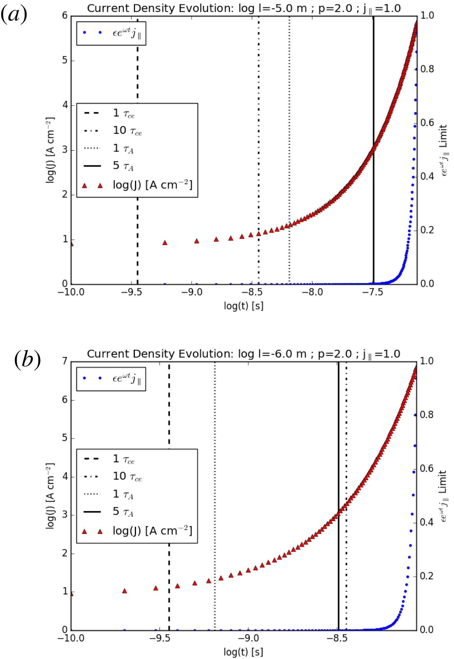
Simulations of spine axis component current density evolution of (4.1) with
 $p=2.0$
,
 $j_{\Vert }=1.0$
,
 $B_{0}=10^{-1}~\text{T}$
and
 $n=10^{24}~\text{m}^{-3}$
, with deuterium plasma. (a) Resistive MHD scale with
 $l=l_{cs}=\unicode[STIX]{x1D716}=10^{-5}$
. The current amplification (left axis) begins to increase significantly after one
 $\unicode[STIX]{x1D70F}_{A}$
(vertical dotted line), well after many electron gyro-periods (
 ${>}10\unicode[STIX]{x1D70F}_{ce}$
). The behaviour exceeds the defined limit of valid behaviour
 $\unicode[STIX]{x1D716}\text{e}^{\unicode[STIX]{x1D714}t}j_{\Vert }<1$
(right axis) after
 $7.4\times 10^{-8}~\text{s}$
(
 ${\sim}11\unicode[STIX]{x1D70F}_{A}$
,
 ${\sim}200\unicode[STIX]{x1D70F}_{ce}$
). The
 $5\unicode[STIX]{x1D70F}_{A}$
threshold is also noted by the vertical solid line. (b) Kinetic scale with
 $l=d_{e}=\unicode[STIX]{x1D716}=10^{-6}$
. The current amplification (left axis) begins to increase significantly after one
 $\unicode[STIX]{x1D70F}_{ce}$
(vertical dotted line) and one
 $\unicode[STIX]{x1D70F}_{A}$
(vertical dotted line), and exceeds the defined limit of valid behaviour
 $\unicode[STIX]{x1D716}\text{e}^{\unicode[STIX]{x1D714}t}j_{\Vert }<1$
(right axis) after
 $8.9\times 10^{-9}~\text{s}$
(
 ${\sim}13\unicode[STIX]{x1D70F}_{A}$
,
 ${\sim}25\unicode[STIX]{x1D70F}_{ce}$
). The
 $10\unicode[STIX]{x1D70F}_{ce}$
threshold is also noted by the vertical dot–dashed line and is notably close in time to the
 $5\unicode[STIX]{x1D70F}_{A}$
threshold (vertical solid line).

4 Numerical analyses of TSR
To further elucidate the anticipated behaviour of the investigated TSR experimental regime, and to gauge the relative importance of resistive MHD versus kinetics, we have completed numerical analyses of the solutions to the linearized, low-
 $\unicode[STIX]{x1D6FD}$
, ideal MHD equations due to perturbations of a potential null point field (Parnell et al.
Reference Parnell, Neukirch, Smith and Priest1997). To study the localized nature of current sheet formation and the time evolution of null point field line structuring, the formulation of Parnell et al. (Reference Parnell, Smith, Neukirch and Priest1996) was expanded to derive a model for a perturbation that induces a component of current in the
 $z$
-direction, corresponding to the spine axis of a null point (Parnell et al.
Reference Parnell, Neukirch, Smith and Priest1997). The authors expressed this current density in the form,
 $$\begin{eqnarray}\boldsymbol{J}=B_{0}\unicode[STIX]{x1D716}\text{e}^{\unicode[STIX]{x1D714}t}(0,0,j_{\Vert })/l\unicode[STIX]{x1D707}_{0},\end{eqnarray}$$
where
 $B_{0}$
is the initial magnetic field,
 $\unicode[STIX]{x1D716}\ll 1$
,
 $l$
is the characteristic length over which reconnection occurs and current sheets form (Dungey Reference Dungey1953) (i.e.
 $l\sim l_{cs}$
for resistive MHD, and
 $l\sim d_{e}$
for kinetics), and the growth rate
 $\unicode[STIX]{x1D714}$
is,
 $$\begin{eqnarray}\unicode[STIX]{x1D714}=|p-1|v_{A}/l.\end{eqnarray}$$
Importantly, the temporal behaviour of (4.1) is only valid provided that
 $\unicode[STIX]{x1D716}\text{e}^{\unicode[STIX]{x1D714}t}j_{\Vert }<1$
(Parnell et al.
Reference Parnell, Neukirch, Smith and Priest1997).
We have solved (4.1) and (4.2) for current sheets on both resistive MHD and kinetic scales of
 $l_{cs}$
and
 $d_{e}$
, respectively. Our magnetic field matrix parametrization following Parnell et al. (Reference Parnell, Smith, Neukirch and Priest1996) uses
 $p=2$
, identical to the TSR simulations of Pontin et al. (Reference Pontin, Al-Hachami and Galsgaard2011), and with current along the spine
 $j_{\Vert }=1$
and
 $q=j_{\bot }=0$
. This numerical parametrization satisfies the constraints of the matrix formulation of Parnell et al. (Reference Parnell, Smith, Neukirch and Priest1996). Other plasma parameters are taken from the TSR regime in table 1. In each case, the parameter
 $\unicode[STIX]{x1D716}\ll 1$
is chosen to be of order
 $l$
.
Figure 6(a) depicts equation (4.1) solutions for the spine axis component of the current density for the resistive MHD length scale of a current sheet width
 $l_{cs}=10^{-5}~\text{m}$
. The collapse of the null point and maximum current amplification occurs after
 $7.4\times 10^{-8}~\text{s}$
, or
 ${\sim}11\unicode[STIX]{x1D70F}_{A}$
and
 ${\sim}200\unicode[STIX]{x1D70F}_{ce}$
. Such Alfvén time scales are consistent with the MHD collapse of 2-D X-line diffusion regions (Imshennik & Syrovatskiǐ Reference Imshennik and Syrovatskiǐ1967; Parnell et al.
Reference Parnell, Neukirch, Smith and Priest1997). However, the electron gyro-periods of
 $1\unicode[STIX]{x1D70F}_{ce}$
and
 $10\unicode[STIX]{x1D70F}_{ce}$
are also shown, and these both occur well prior to even
 $1\unicode[STIX]{x1D70F}_{A}$
. Therefore, the energization of electrons on diffusive time scales at these length scales will only break the frozen-in condition very slowly, if at all, since it is possible that electron energization may be damped away before resistive effects, and thus reconnection, can take over. Since these equations are based on ideal MHD, the current densities reached toward the end of this behaviour
 ${\gtrsim}10~\text{kA}~\text{cm}^{-2}$
can be considered an upper limit of any true laboratory plasma behaviour in our system. That is, the unique difference to other set-ups is the use of a dense deuterium plasma that will introduce additional resistivity to current amplification processes.
Figure 6(b) depicts identical equation (4.1) solutions for the spine axis component of the current density for the kinetic length scale of a current sheet width equal to the electron skin depth
 $d_{e}=10^{-6}~\text{m}$
. The collapse of the null point and its resulting current amplification occurs after
 $8.9\times 10^{-9}~\text{s}$
, or
 ${\sim}13\unicode[STIX]{x1D70F}_{A}$
and
 ${\sim}25\unicode[STIX]{x1D70F}_{ce}$
. Even on a smaller length scale, the Alfvén time scales are still consistent with MHD collapse. Fortunately, in comparison to the resistive MHD-scale solution, both the
 $1\unicode[STIX]{x1D70F}_{ce}$
:
 $1\unicode[STIX]{x1D70F}_{A}$
and
 $10\unicode[STIX]{x1D70F}_{ce}$
:
 $5\unicode[STIX]{x1D70F}_{A}$
milestones occur close together on kinetic scales. Therefore, kinetic effects are considered to be important in the considered TSR plasma regime, as electron energization corresponds to Alfvén wave perturbations, and fast reconnection shorter than the time scales predicted by resistive diffusion can occur. Such a kinetic approach is further justified by the ratio of the electron gyrofrequency to the electron plasma frequency
 $\unicode[STIX]{x1D714}_{ce}/\unicode[STIX]{x1D714}_{ce}$
in table 1. Since
 $\unicode[STIX]{x1D714}_{pe}\gg \unicode[STIX]{x1D714}_{ce}$
, current sheets of order
 $d_{e}$
are anticipated to be able to form within the TSR dense plasma regime.
As a final note on these predicted time scales, the described TSR experiment featuring a rigidly controlled isolated null point is obviously an open geometry along the spine axis that will not feature separators connecting pairs of nulls. This open geometry will not confine plasma well. However, plasma and current sheet evolution are the features we are aiming to control, not confinement. Thus, the predicted rapid time scales of reconnection, likely faster than
 $\unicode[STIX]{x1D70F}_{D}$
, may be difficult to diagnose from the first approximations presented here. We anticipate our analyses presented herein (e.g. table 1) to be a springboard for future analyses that will further constrain the presented experimental geometry.
5 Discussion
The 3-D TSR mode is a qualitative result that has not yet been achieved in existing magnetic reconnection experiments. As such, we have explored the feasibility of a novel laboratory set-up that can initialize, and subsequently break, the frozen-in flux condition for inducing the process of TSR within both resistive MHD and kinetic length scales. Leveraging existing robust TSR simulations (Pontin & Galsgaard Reference Pontin and Galsgaard2007; Pontin et al. Reference Pontin, Al-Hachami and Galsgaard2011) has allowed us to identify and model components of existing technology that can mimic the dynamics necessary for both setting up the static potential null point field and for providing the unique magnetic field perturbation that induces the onset of reconnection (figure 5). The calculation of the requisite plasma parameters and the application of a model of magnetic field and plasma behaviour (Parnell et al. Reference Parnell, Smith, Neukirch and Priest1996, Reference Parnell, Neukirch, Smith and Priest1997) show that spine-aligned current amplification about an isolated magnetic null point will take place of the order of a few electron gyro-periods and Alfvén times (figure 6).
The numerical results of figure 6 suggest that fast reconnection on the small spatial scales of this TSR set-up will likely occur on kinetic scales (
 ${\sim}25\unicode[STIX]{x1D70F}_{ce}$
) within current sheets also featuring resistive MHD effects (
 ${\sim}13\unicode[STIX]{x1D70F}_{A}$
). It is important to consider the implications of these time scales in the selection of enabling technology components (§ 2). The DPF plasma sheath discussed in § 2 that contains both the in-situ plasma for reconnection as well as the necessary azimuthal magnetic field perturbation has an axial propagation lifetime of the order of tens of microseconds (Lee & Serban Reference Lee and Serban1996) (
 ${\sim}10~\unicode[STIX]{x03BC}\text{s}~\text{cm}^{-1}$
). Therefore, after the DPF forms the plasma sheath, its flat-top-phase axial propagation due to its self
 $\boldsymbol{J}\times \boldsymbol{B}$
force, due to (2.3), is of the order of
 ${\sim}100\unicode[STIX]{x1D70F}_{A}$
or
 ${\sim}10^{3}\unicode[STIX]{x1D70F}_{ce}$
for the dense deuterium plasma we considered, providing sufficient time for the onset of TSR dynamics (
 ${\sim}13\unicode[STIX]{x1D70F}_{A}$
or
 ${\sim}25\unicode[STIX]{x1D70F}_{ce}$
).
Since the described laboratory set-up will provide rapid perturbations to a capacitively coupled plasma in a potential null point field, we can anticipate some experimental signatures of interest. First and foremost, the narrow current sheet width of
 ${\lesssim}20~\unicode[STIX]{x03BC}\text{m}$
forming within rapid temporal scales of
 ${\lesssim}10~\text{ns}$
in our first-order predictions (table 1) will require sophisticated diagnostic equipment to decipher. Effective nanosecond and even picosecond-level soft X-ray spectroscopic interferometry of dense plasmas up to
 $n\sim 10^{24}~\text{m}^{-3}$
(Filevich et al.
Reference Filevich, Rocca, Hammarsten, Jankowska, Marconi, Smith, Keenan, Dunn, Moon and Shlyaptsev2003, Reference Filevich, Rocca, Marconi, Smith, Dunn, Keenan, Hunter, Moon, Nilsen and Ng2004; Grava et al.
Reference Grava, Purvis, Filevich, Marconi, Rocca, Dunn, Moon and Shlyaptsev2008) is one such diagnostic system that may be able to effectively diagnose TSR in the described experimental set-up. Spatial resolutions of
 ${\sim}2~\unicode[STIX]{x03BC}\text{m}$
(Filevich et al.
Reference Filevich, Rocca, Hammarsten, Jankowska, Marconi, Smith, Keenan, Dunn, Moon and Shlyaptsev2003) using compact soft X-ray lasers with high repetition frequency may also be able to image plasma dynamics during TSR. Two-photon laser-induced fluorescence (TALIF; e.g. Thakur et al.
Reference Thakur, Adriany, Gosselin, McKee, Scime, Sears and Tynan2016, Schmidt et al.
Reference Schmidt, Sands, Scofield, Gord and Roy2017) produces fs-level laser pulses resulting in sub-ns temporal resolution (Schmidt et al.
Reference Schmidt, Sands, Scofield, Gord and Roy2017) of plasma diagnostics such as axial velocity, velocity shear and ion temperature profiles (Thakur et al.
Reference Thakur, Adriany, Gosselin, McKee, Scime, Sears and Tynan2016). TALIF is also able to make magnetic field intensity measurements within the plasma by observing wavelength-dependent Zeeman splitting via left and right circular polarization measurements (e.g. Noonan, Jones & Ottinger Reference Noonan, Jones and Ottinger1997, Ngom et al.
Reference Ngom, Smith, Huang and Gallimore2008, Thakur et al.
Reference Thakur, Adriany, Gosselin, McKee, Scime, Sears and Tynan2016). These TALIF measurements may resolve the rapid,
 ${\sim}$
ns-level magnetic field line slippages in the fan plane centred on the spine within the toroidal plasma sheath as TSR manifests. Use of such remote laser systems to diagnose TSR in the described set-up can eliminate the need for intrusive Langmuir and B-dot probes with lower temporal resolution.
The choice of deuterium parameters in this study is based on established DPF practices (e.g. Lee & Serban Reference Lee and Serban1996, Bures et al. Reference Bures, Krishnan, Madden and Blobner2010, Reference Bures, Krishnan and James2012, Abdou et al. Reference Abdou, Ismail, Mohamed, Lee, Saw and Verma2012, Mitrofanov et al. Reference Mitrofanov, Krauz, Kubes, Scholz, Paduch and Zielinska2014). However, the use of helium, molecular oxygen (Schmidt et al. Reference Schmidt, Sands, Scofield, Gord and Roy2017) and argon (Thakur et al. Reference Thakur, Adriany, Gosselin, McKee, Scime, Sears and Tynan2016) energy-level transitions are standard for TALIF measurements, and the use of heavier ions may be necessary for employing proper diagnostics. DPFs can operate with heavy ions such as neon (Caballero Bendixsen et al. Reference Caballero Bendixsen, Bott-Suzuki, Cordaro, Krishnan, Chapman, Coleman and Chittenden2016) and argon (Heo & Park Reference Heo and Park2002) and can be diagnosed with laser interferometry (Caballero Bendixsen et al. Reference Caballero Bendixsen, Bott-Suzuki, Cordaro, Krishnan, Chapman, Coleman and Chittenden2016). The use of a heavier ion may have the added benefit of slowing down the TSR process, as it would increase the diffusion time scale, ion skin depth, ion gyroradius and ion gyroperiod of the plasma. While this drawing out of the reconnection process would likely make plasma diagnostics easier, there is a corresponding increase in resistivity of the plasma (lower Lundquist number). Therefore, careful considerations must be made to reach a balance between slowing down TSR and creating a more resistive plasma.
Spine-localized current peaks signify the onset of non-ideal processes (i.e. reconnection) that dissipate built-up stress (Pontin & Galsgaard Reference Pontin and Galsgaard2007). This reconnection process, that is initiated by the twisting of fan field lines, manifests as an energy balance between the perturbative motions and the rotational field line slippages due to resistive diffusion (Pontin et al. Reference Pontin, Al-Hachami and Galsgaard2011). Interestingly, the authors of previous robust TSR simulations (Pontin & Galsgaard Reference Pontin and Galsgaard2007; Pontin et al. Reference Pontin, Al-Hachami and Galsgaard2011) note that a continually driven rotational perturbation should result in the persistence of the resulting spine-localized current for the period of the boundary controlled driving. Therefore, if these perturbations can be continuously applied in a temporally optimized fashion, a quasi-steady state of enhanced spine-localized current can be reached between the rotational twist of the perturbation field and the rotational slippage (Pontin Reference Pontin2011). Such quasi-steady state operations may be possible since pulse-power-driven DPF technology is approaching operational frequencies of 100 Hz (Bures et al. Reference Bures, Krishnan and James2012). This optimization is a subject for further investigation.
Such experimentally induced current sheets may also have significant implications on the ability to study plasma sheets in a non-equilibrium self-organized state (Chang Reference Chang1992, Reference Chang1999; Valdivia et al. Reference Valdivia, Rogan, Munoz and Toledo2006). Rotational plasma flows, helical current sheets, and spine-aligned current amplifications are manifestations of a system driven to criticality (Bak, Tang & Wiesenfeld Reference Bak, Tang and Wiesenfeld1987) as the rotational slippages of TSR manifest as a repeatable balance between nonlinear plasma resistivity and intermittent dissipation of a self-organized state. An understanding of this self-organization balance is a key to deciphering the evolution of reconnection events in astrophysical plasmas. In fact, it can be argued that the behaviour of energy dissipation in TSR is more of a property of a self-organized critical state than it is a property of the TSR process itself (Valdivia et al. Reference Valdivia, Rogan, Munoz and Toledo2006). This self-organization, and an ability to control such organization in a TSR experiment, can have far reaching implications for both turbulent dissipation and turbulence suppression in reconnecting plasmas, as well as other laboratory plasma confinement operations, such as fusion reactors (Grasso et al. Reference Grasso, Lazzaro, Borgogno and Comisso2016).
The presented estimates for a previously unexplored class of 3-D reconnection mode experimentation represents a significant step forward in our abilities to mimic plasma dynamics observed in astrophysical plasmas, e.g. solar atmosphere (Török et al.
Reference Török, Aulanier, Schmieder, Reeves and Golub2009), planetary magnetospheres (Wendel & Adrian Reference Wendel and Adrian2013; Olshevsky et al.
Reference Olshevsky, Divin, Eriksson, Markidis and Lapenta2015) and galactic nuclei (Nalewajko Reference Nalewajko2016). The experimental set-up as described here, where both the plasma for reconnection and the necessary perturbation are produced in situ (figures 4 and 5), may signify an important step forward in the formation of coherent dense plasma sheets that can be formed via reconnection along open field lines. As such, our TSR system could hold similar impacts for technology advancements, particularly in consideration of the recent work of Cazzola et al. (Reference Cazzola, Curreli, Markidis and Lapenta2016) on the novel concept of utilizing magnetic reconnection as a mechanism for high specific impulse in-space propulsion (Chesny Reference Chesny2013). While their analysis was based on X-point plasma outflows of the order of the local
 $v_{A}$
that are possible in existing spheromak and tokamak-style laboratory configurations (Cazzola et al.
Reference Cazzola, Curreli, Markidis and Lapenta2016), any practical, mass-constrained spacecraft application would require explicit control of a centimetre-scale highly compact plasma sheet concentrated along open magnetic field lines, such as that explored here, that can propagate far from the reconnection region. The TSR mode has been suggested to be a highly efficient mechanism for accelerating injected particles to spine-aligned relativistic velocities on fast
 ${\sim}$
ms time scales (Hosseinpour Reference Hosseinpour2014; Hosseinpour, Mehdizade & Mohammadi Reference Hosseinpour, Mehdizade and Mohammadi2014). Issues of plasma confinement and losses present in other plasma propulsion systems could also be significantly decreased, as TSR mode charged particle acceleration is only efficient close to the rotational perturbation region (Hosseinpour Reference Hosseinpour2014), e.g. where the in situ DPF plasma sheath is created in this system. A reconnection-based propulsion system may also be optimized for long-duration operation by achieving the quasi-steady state, spine-aligned flows discussed above (Pontin Reference Pontin2011).
6 Conclusion
This initial feasibility study has opened the door to a possible new class of laboratory studies investigating the nature of 3-D magnetic reconnection. The magnetic field dynamics addressed herein opens up a wide variety of further individual aspects deserving attention. We stress that the technologies described here are simply candidate hardware for such experimentation, and by no means do they encompass the range of possible components that could be used to induce TSR. As with any laboratory set-up, varying types of hardware components and component geometries can be utilized for achieving the same particle dynamics, so further efforts are needed to optimize and constrain the range of technologies and their geometries that can be used for the induction of TSR. Further investigations into the optimization of hardware components that could be used to induce TSR, including robust computational models, will likely have to take into account important effects such as MHD turbulence, collisional shocks, material degradation effects due to turbulent plasma motions, the balance between pulsed power and maintaining idealized flows and effects of partial ionization, etc.
An alteration in the sequence of operation may also be considered for this TSR experiment. Instead of the DPF capacitor bank discharge occurring within an ambient null point magnetic field, the sequence may be reversed. With the component geometries unchanged, the null point field can be energized by the conducting coil during the flat-top phase of the DPF plasma sheath that is propagating at an axial speed of
 ${\sim}10~\text{us}~\text{cm}^{-1}$
. It is anticipated that this reversed sequence of events will have the same effect of a circular perturbation to a null point field consistent with TSR, but with the flat-top plasma being established prior to the perturbation of the null point field. The use of kinetic particle-in-cell methods can be used to simulate both the boundary conditions of hardware components (Guillory et al.
Reference Guillory, Rose, Lerner, Kusse and Hammer2009) and the complex plasma dynamics of resistive magnetic reconnection (Dahlin, Drake & Swisdak Reference Dahlin, Drake and Swisdak2014) in order to resolve outstanding issues. Optimization of the full range of hardware parameters is necessary to efficiently drive TSR and study the resulting current densities and plasma flows.
Extensions of this experimental set-up can also be considered. The addition of a third conducting coil in the geometry of figure 4 would form a second adjacent magnetic null. Such a configuration would necessarily result in the formation of a positive–negative null pair. The orientation of the DPF would require its main axial direction to point in the direction of the null pair (separator), and its operation may result in separator reconnection. An additional geometrical alteration could be the rotation of the DPF device by
 $90^{\circ }$
through the spine axis. The circular perturbation to the spine fan axis may replicate the dynamics needed to induce the spine fan 3-D reconnection mode (Thurgood, Pontin & McLaughlin Reference Thurgood, Pontin and McLaughlin2017, see figure 1 within). Finally, and equally as important, the possibility for a new frontier of centimetre-scale plasma physics experiments within a volume of
 ${\lesssim}1~\text{m}^{3}$
, as presented by this work, could hold significant potential for broadening the academic and industrial players carrying out active plasma physics research.
Acknowledgements
D.L.C. would like to thank P. Champey and C. Wang for helpful discussions on diagnostic systems, and G.A. Levin for helpful comments. N.B.O. thanks the University of the Virgin Islands.