2.1 Fluid formulation

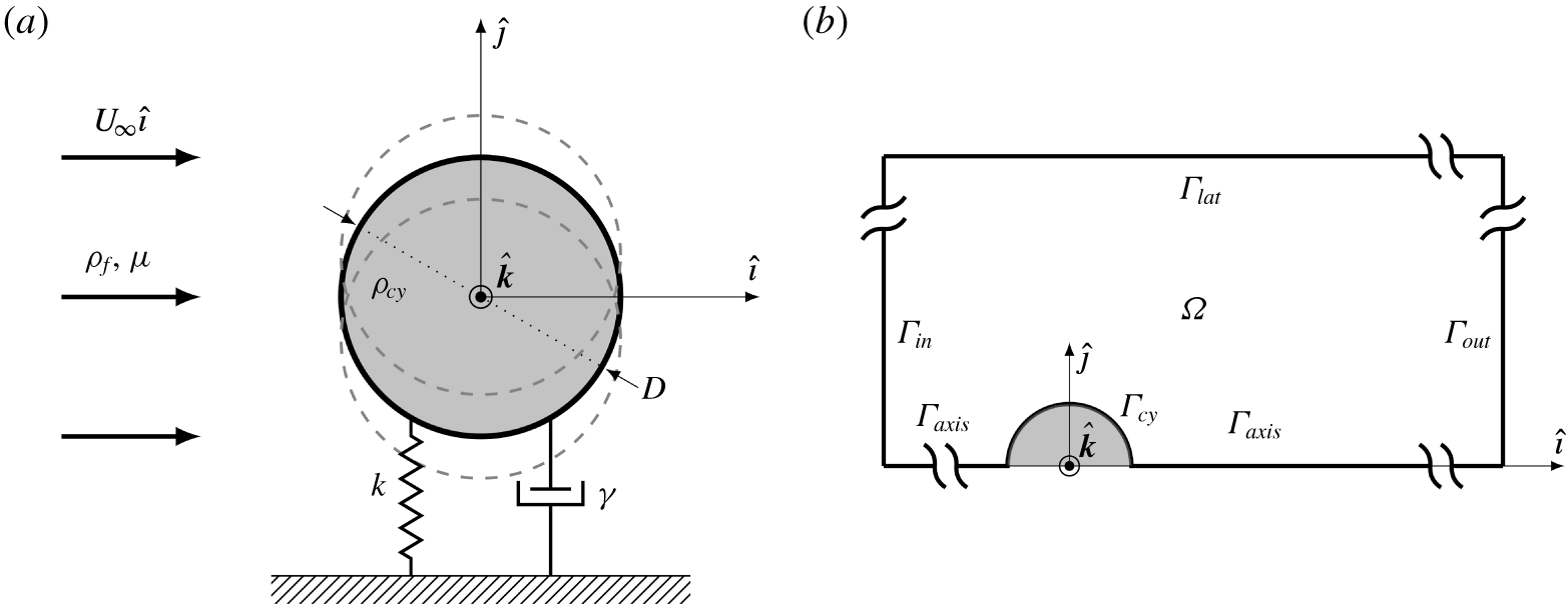
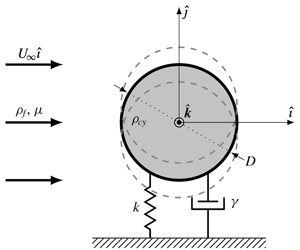
A Cartesian coordinate system is used with its origin at the centre of the cylinder, which travels with the cylinder motion. The $\hat{\boldsymbol{\imath }}$-axis is considered parallel to the streamwise direction, whereas the $\hat{\boldsymbol{\jmath }}$-axis points laterally, as depicted in figure 1(a). The spatial and temporal domains are represented by $\unicode[STIX]{x1D6FA}\in \mathbb{R}^{2}$ and $[0,T]$, respectively. Following the formulation of Mougin & Magnaudet (Reference Mougin and Magnaudet2002), which consists of expressing the absolute velocity $\boldsymbol{u}$ in the relative frame moving with the cylinder, the flow around the cylinder can be described by the non-dimensional laminar incompressible Navier–Stokes equations, defined as

(2.1a)$$\begin{eqnarray}\displaystyle & \displaystyle \unicode[STIX]{x2202}_{t}\boldsymbol{u}+((\boldsymbol{u}-\dot{\unicode[STIX]{x1D701}}\hat{\boldsymbol{\jmath }})\boldsymbol{\cdot }\unicode[STIX]{x1D735})\boldsymbol{u}=-\unicode[STIX]{x1D735}p+2Re^{-1}\unicode[STIX]{x1D735}\boldsymbol{\cdot }\unicode[STIX]{x1D63F}(\boldsymbol{u}), & \displaystyle\end{eqnarray}$$

(2.1b)$$\begin{eqnarray}\displaystyle & \displaystyle \unicode[STIX]{x1D735}\boldsymbol{\cdot }\boldsymbol{u}=0, & \displaystyle\end{eqnarray}$$

$\unicode[STIX]{x1D6FA}\times [0,T]$

$\unicode[STIX]{x1D63F}(\boldsymbol{u})\overset{\underset{\text{def}}{}}{=}1/2(\unicode[STIX]{x1D735}\boldsymbol{u}+\unicode[STIX]{x1D735}\boldsymbol{u}^{\text{T}})$

$p$

$\unicode[STIX]{x1D70C}_{f}$

$\unicode[STIX]{x1D701}$

$Re$

$Re=DU_{\infty }/\unicode[STIX]{x1D708}$

$D$

$U_{\infty }$

$\unicode[STIX]{x1D708}$

The domain limits are depicted in figure 1(b). To take advantage of the problem’s symmetry, a half-domain representation is implemented with the proper boundary conditions on the axis in order to obtain the symmetric or anti-symmetric (periodic) solutions. The remaining boundary conditions are posed as

(2.2a)$$\begin{eqnarray}\displaystyle & \displaystyle \boldsymbol{u}=-\dot{\unicode[STIX]{x1D701}}\hat{\boldsymbol{\jmath }}\quad \text{on }\unicode[STIX]{x1D6E4}_{cy}, & \displaystyle\end{eqnarray}$$

(2.2b)$$\begin{eqnarray}\displaystyle & \displaystyle \boldsymbol{u}=U_{\infty }\hat{\boldsymbol{\imath }}\quad \text{on }\unicode[STIX]{x1D6E4}_{in}\cup \unicode[STIX]{x1D6E4}_{lat}, & \displaystyle\end{eqnarray}$$

(2.2c)$$\begin{eqnarray}\displaystyle & \displaystyle [-\unicode[STIX]{x1D735}p+2Re^{-1}\unicode[STIX]{x1D63F}(\boldsymbol{u})]\boldsymbol{\cdot }\boldsymbol{n}=0\quad \text{on }\unicode[STIX]{x1D6E4}_{out}, & \displaystyle\end{eqnarray}$$

$\boldsymbol{n}$

Figure 1.

(a) A schematic showing the dimensional input variables of the damped spring–mass cylinder and the coordinate system of the problem, and (b) a schematic representation of the computational domain and boundary conditions.

2.2 Structure model: forced and coupled formulations

The effect of the motion of the cylinder on the fluid flow appears through the transverse velocity $\dot{\unicode[STIX]{x1D701}}(t)$ of the cylinder which is present in both the Navier–Stokes equations (2.1) and the boundary condition (2.2a).

For the forced case, the displacement is imposed by a sinusoidal motion under the form $\dot{\unicode[STIX]{x1D701}}=|\dot{\unicode[STIX]{x1D701}}_{F}|\sin (\unicode[STIX]{x1D714}_{F}t)$, where $\unicode[STIX]{x1D714}_{F}$ is the imposed frequency.

For the coupled case, the linear equation modelling the motion of the cylinder is posed as

(2.3)$$\begin{eqnarray}\ddot{\unicode[STIX]{x1D701}}+\frac{4\unicode[STIX]{x03C0}\unicode[STIX]{x1D6FE}}{U^{\ast }}\dot{\unicode[STIX]{x1D701}}+\left(\frac{2\unicode[STIX]{x03C0}}{U^{\ast }}\right)^{2}\unicode[STIX]{x1D701}=\frac{2C_{y}(t)}{\unicode[STIX]{x03C0}m^{\ast }},\end{eqnarray}$$

where $\unicode[STIX]{x1D6FE}$ is the damping ratio, $m^{\ast }=\unicode[STIX]{x1D70C}_{cy}/\unicode[STIX]{x1D70C}_{f}$, is the mass ratio between the cylinder and fluid densities, $U^{\ast }=U_{\infty }/(f_{N}D)=2\unicode[STIX]{x03C0}U_{\infty }\sqrt{m_{cy}/k}/D$ is the reduced velocity and $C_{y}(t)=F_{y}(t)/(0.5\unicode[STIX]{x1D70C}U_{\infty }^{2}D)$ is the vertical force coefficient, where $m_{cy}$ and $k$ are the cylinder mass and the spring stiffness, respectively, and $F_{y}(t)$ is the vertical force. The latter is calculated by integrating the stress on the boundary of the cylinder

(2.4)$$\begin{eqnarray}C_{y}(t)=\frac{2F_{y}(t)}{\unicode[STIX]{x1D70C}U_{\infty }^{2}D}=2\int _{\unicode[STIX]{x1D6E4}_{cy}}2\{(-p\boldsymbol{n}+2Re^{-1}\unicode[STIX]{x1D63F}(\boldsymbol{u})\boldsymbol{\cdot }\boldsymbol{n})\boldsymbol{\cdot }\hat{\boldsymbol{\jmath }}\}\,\text{d}\unicode[STIX]{x1D6E4}_{cy},\end{eqnarray}$$

where the factor 2 accounts for the fact that a half-domain is used.

2.3 Linearised Navier–Stokes equations

In the framework of linearised Navier–Stokes equations, the fluid flow, denoted $\boldsymbol{q}=(\boldsymbol{u},p)^{\text{T}}$, is decomposed as

(2.5)$$\begin{eqnarray}\boldsymbol{q}=\boldsymbol{q}_{b}+\frac{\unicode[STIX]{x1D716}}{2}(\hat{\boldsymbol{q}}\,\text{e}^{-\text{i}\unicode[STIX]{x1D714}t}+\text{c.c.}),\end{eqnarray}$$

where $\boldsymbol{q}_{b}=(\boldsymbol{u}_{b},p_{b})^{\text{T}}$ is the steady base flow, $\unicode[STIX]{x1D716}$ is a small parameter, $\hat{\boldsymbol{q}}$ is the perturbation in an ‘eigenmode form’ with $\text{c.c.}$ standing for the complex conjugate and $\unicode[STIX]{x1D714}$ is the complex eigenvalue. The base flow $\boldsymbol{q}_{b}$ is the solution of the time-independent version of the Navier–Stokes equations, which are detailed in appendix B.

Similarly, the cylinder velocity $\dot{\unicode[STIX]{x1D701}}(t)$ and the dimensionless force $C_{y}(t)$ will be expressed under the same ‘eigenmode form’

(2.6a,b)$$\begin{eqnarray}\dot{\unicode[STIX]{x1D701}}(t)=\unicode[STIX]{x1D716}\frac{\hat{\dot{\unicode[STIX]{x1D701}}}\,\text{e}^{-\text{i}\unicode[STIX]{x1D714}t}+\text{c.c.}}{2},\quad C_{y}(t)=\unicode[STIX]{x1D716}\frac{{\hat{C}}_{y}\,\text{e}^{-\text{i}\unicode[STIX]{x1D714}t}+\text{c.c.}}{2}.\end{eqnarray}$$

The eigenmode ansatz (2.5) and (2.6) will be used for both the forced and the coupled problems, so that a difference in the $\unicode[STIX]{x1D714}$ can be interpreted as follows.

1. (i) For the forced problem, $\unicode[STIX]{x1D714}$ is the frequency of the imposed motion of the cylinder and will generally be considered as real (and noted $\unicode[STIX]{x1D714}\equiv \unicode[STIX]{x1D714}_{F}$).

2. (ii) For the coupled problem, on the other hand, $\unicode[STIX]{x1D714}$ is the eigenvalue and is generally expected to be a complex number ($\unicode[STIX]{x1D714}=\unicode[STIX]{x1D714}_{r}+\text{i}\unicode[STIX]{x1D714}_{i}$). Note that the imaginary part $\unicode[STIX]{x1D714}_{i}$ corresponds to the amplification rate, and its sign defines whether the solution decays or grows over time, representing a stability criterion of the eigenmode.

2.3.1 Linearised forced problem

For the forced problem, $\hat{\boldsymbol{q}}$ will be noted $\hat{\boldsymbol{q}}_{F}$ and the linearised Navier–Stokes equations can be set under the following form:

(2.7)$$\begin{eqnarray}(\unicode[STIX]{x1D63C}_{ff}-\text{i}\unicode[STIX]{x1D714}_{F}\unicode[STIX]{x1D63D}_{ff})\hat{\boldsymbol{q}}_{F}=\hat{\dot{\unicode[STIX]{x1D701}}}_{F}\unicode[STIX]{x1D654},\end{eqnarray}$$

where $\unicode[STIX]{x1D63C}_{ff}$ and $\unicode[STIX]{x1D63D}_{ff}$ are the fluid and mass operators and the operator $\unicode[STIX]{x1D654}$ represents the effect of the cylinder motion on the fluid (which appears both as a volumetric term in the Navier–Stokes equations and in the boundary conditions). The weak form expressions for these operators are given in appendix B.

Once this problem is solved, the vertical force coefficient can be extracted as ${\hat{C}}_{y}=\unicode[STIX]{x1D647}(\hat{\boldsymbol{q}}_{F})$ where $\unicode[STIX]{x1D647}$ is the ‘vertical force coefficient’ operator, also defined in appendix B. The mechanical impedance $Z(\unicode[STIX]{x1D714}_{F})$ can now be defined as the ratio between vertical force coefficient amplitude and the cylinder velocity amplitude

(2.8)$$\begin{eqnarray}Z(\unicode[STIX]{x1D714}_{F})=-\frac{{\hat{C}}_{y}}{\hat{\dot{\unicode[STIX]{x1D701}}}}=\frac{{\hat{C}}_{y}}{\text{i}\unicode[STIX]{x1D714}_{F}\hat{\unicode[STIX]{x1D701}}}.\end{eqnarray}$$

As shown in the next sections, the concept of impedance provides a useful way to characterise the problem in both the forced case and the coupled case. Moreover, it provides a link with problems in electricity and acoustics where such a concept is widely used. In particular, the real and imaginary part of the impedance ($Z=Z_{r}+\text{i}Z_{i}$) can be identified with the resistance and reactance, respectively.

Note that, for the forced case, the mechanical impedance can be formally defined as $Z(\unicode[STIX]{x1D714}_{F})=-\unicode[STIX]{x1D647}(\hat{\boldsymbol{q}}_{F})[(\unicode[STIX]{x1D63C}_{ff}-\text{i}\unicode[STIX]{x1D714}_{F}\unicode[STIX]{x1D63D}_{ff})\hat{\boldsymbol{q}}_{F}]^{-1}\boldsymbol{\cdot }\unicode[STIX]{x1D654}$, so the computation of this quantity after discretisation of the operators is straightforward.

2.3.2 Linearised coupled problem

In the coupled problem, the one-way coupling between fluid and the cylinder structure is still represented by (2.7) (with a generally complex $\unicode[STIX]{x1D714}$ instead of the real $\unicode[STIX]{x1D714}_{F}$), but the cylinder displacement $\hat{\unicode[STIX]{x1D701}}$ is now related to the vertical force coefficient ${\hat{C}}_{y}$ through the dynamical equation (2.3). The whole set of equations can now be written in eigenvalue form considering the state vector $\hat{\boldsymbol{q}}_{CP}=(\hat{\boldsymbol{q}},\hat{\unicode[STIX]{x1D701}},\hat{\dot{\unicode[STIX]{x1D701}}},\hat{\ddot{\unicode[STIX]{x1D701}}})^{\text{T}}$ as follows:

(2.9)$$\begin{eqnarray}(\unicode[STIX]{x1D63C}-\text{i}\unicode[STIX]{x1D714}\unicode[STIX]{x1D63D})\hat{\boldsymbol{q}}_{CP}=\mathbf{0},\end{eqnarray}$$

with

(2.10a,b)$$\begin{eqnarray}\unicode[STIX]{x1D63C}=\left[\begin{array}{@{}cccc@{}}\unicode[STIX]{x1D63C}_{ff} & 0 & -\unicode[STIX]{x1D654} & 0\\ 0 & 0 & 1 & 0\\ 0 & 0 & 0 & 1\\ \displaystyle \frac{2}{\unicode[STIX]{x03C0}m^{\ast }}\unicode[STIX]{x1D647} & \displaystyle -\left(\frac{2\unicode[STIX]{x03C0}}{U^{\ast }}\right)^{2} & \displaystyle -\frac{4\unicode[STIX]{x03C0}\unicode[STIX]{x1D6FE}}{U^{\ast }} & -1\end{array}\right]\quad \text{and}\quad \unicode[STIX]{x1D63D}=\left[\begin{array}{@{}cccc@{}}\unicode[STIX]{x1D63D}_{ff} & 0 & 0 & 0\\ 0 & 1 & 0 & 0\\ 0 & 0 & 1 & 0\\ 0 & 0 & 0 & 0\end{array}\right].\end{eqnarray}$$

3.1 Linking energy transfer and impedance

Following the work done by Morse & Williamson (Reference Morse and Williamson2009b) and Navrose & Mittal (Reference Mittal2016), the net energy transfer from the fluid to the cylinder, over a period $T$, can be defined as

(3.1)$$\begin{eqnarray}E_{transfer}=\int _{0}^{T}[C_{y}(t)\dot{\unicode[STIX]{x1D701}}(t)]\,\text{d}t.\end{eqnarray}$$

Considering a forced problem (with a real $\unicode[STIX]{x1D714}_{F}$) with displacement $\unicode[STIX]{x1D701}(t)$ and dimensionless force $C_{y}(t)$ given by (2.6), the integration over one period ($T=2\unicode[STIX]{x03C0}/\unicode[STIX]{x1D714}_{F}$) leads to (see appendix A)

(3.2)$$\begin{eqnarray}E_{transfer}=-\unicode[STIX]{x03C0}|\hat{\unicode[STIX]{x1D701}}|^{2}\unicode[STIX]{x1D714}_{F}Z_{r}(\unicode[STIX]{x1D714}_{F}).\end{eqnarray}$$

The property of $E_{transfer}$ being positive for some real value of $\unicode[STIX]{x1D714}_{F}$ has been proposed by Morse & Williamson (Reference Morse and Williamson2009b) as an instability criterion for the fully coupled problem. This criterion is usually expressed in terms of the phase shift $\unicode[STIX]{x1D719}$ between the vertical force coefficient and the cylinder displacement

(3.3)$$\begin{eqnarray}E_{transfer}>0\quad \Longleftrightarrow \quad \unicode[STIX]{x1D719}=\text{arg}({\hat{C}}_{y}/\hat{\unicode[STIX]{x1D701}})\in [0,\unicode[STIX]{x03C0}].\end{eqnarray}$$

The concept of impedance introduced in the previous section, allows to express this instability criterion in an alternative form

(3.4)$$\begin{eqnarray}E_{transfer}>0\quad \Longleftrightarrow \quad Z_{r}(\unicode[STIX]{x1D714}_{F})<0\quad \text{for some real }\unicode[STIX]{x1D714}_{F}.\end{eqnarray}$$

This second expression makes sense when recalling that the real part of the impedance is analogous to an electrical resistance; indeed the possibility of negative resistance is a well known source of instability in electrical circuits (see Conciauro & Puglisi Reference Conciauro and Puglisi1981).

3.2 Link between forced and coupled problems

Although the criterion discussed in the previous section is physically intuitive, it is not totally rigorous as it uses the impedance computed for some real frequency $\unicode[STIX]{x1D714}_{F}$ to predict an instability, which corresponds to a solution of the coupled problem with some complex $\unicode[STIX]{x1D714}$. The situation can be clarified when considering the impedance defined by (2.8) as an analytical function of the complex variable $\unicode[STIX]{x1D714}$. Plugging this definition into the dynamical equation (2.3) leads to the following expression:

(3.5)$$\begin{eqnarray}-\unicode[STIX]{x1D714}^{2}-\frac{4\unicode[STIX]{x03C0}\unicode[STIX]{x1D6FE}\text{i}\unicode[STIX]{x1D714}}{U^{\ast }}+\left(\frac{2\unicode[STIX]{x03C0}}{U^{\ast }}\right)^{2}-\frac{2\text{i}\unicode[STIX]{x1D714}Z(\unicode[STIX]{x1D714})}{\unicode[STIX]{x03C0}m^{\ast }}=0.\end{eqnarray}$$

Mathematically, the eigenvalues of the coupled problem (2.9) correspond to the complex zeros of this constitutive relation. The objective of this section is to derive a prediction of these eigenvalues as a function of the most easily computed and physically meaningful values of $Z$ along the real $\unicode[STIX]{x1D714}$-axis (i.e. based on the forced problem).

We first note that a condition for the existence of purely real solutions of the relation (3.5) is that the damping rate is zero $(\unicode[STIX]{x1D6FE}=0)$ and the impedance is purely imaginary ($Z_{r}=0$). This leads to the assumption of the existence of nearly real solutions in the asymptotic limit corresponding to the following hypotheses:

(3.6a)$$\begin{eqnarray}\displaystyle & \displaystyle |Z_{r}|\ll |Z_{i}|, & \displaystyle\end{eqnarray}$$

(3.6b)$$\begin{eqnarray}\displaystyle & \displaystyle \unicode[STIX]{x1D6FE}\ll 1. & \displaystyle\end{eqnarray}$$

(3.7)$$\begin{eqnarray}\unicode[STIX]{x1D714}=\unicode[STIX]{x1D714}_{F}+\unicode[STIX]{x1D714}^{(1)},\quad \text{with }|\unicode[STIX]{x1D714}^{(1)}|\ll |\unicode[STIX]{x1D714}_{F}|\text{and }\unicode[STIX]{x1D714}_{F}\in \{R.\end{eqnarray}$$

Introducing these hypotheses into equation (3.5) and performing a Taylor development in terms of the quantities assumed small leads to

(3.8)$$\begin{eqnarray}\displaystyle & & \displaystyle \left[-\unicode[STIX]{x1D714}_{F}^{2}+\left(\frac{2\unicode[STIX]{x03C0}}{U^{\ast }}\right)^{2}+\frac{2\unicode[STIX]{x1D714}_{F}Z_{i}(\unicode[STIX]{x1D714}_{F})}{\unicode[STIX]{x03C0}m^{\ast }}\right]\nonumber\\ \displaystyle & & \displaystyle \quad +\,\left[-2\unicode[STIX]{x1D714}_{F}\unicode[STIX]{x1D714}^{(1)}-\frac{4\unicode[STIX]{x03C0}\unicode[STIX]{x1D6FE}\text{i}\unicode[STIX]{x1D714}_{F}}{U^{\ast }}+\frac{2\unicode[STIX]{x1D714}_{F}}{\unicode[STIX]{x03C0}m^{\ast }}\left(-\left.\frac{\unicode[STIX]{x2202}Z}{\unicode[STIX]{x2202}\unicode[STIX]{x1D714}}\right|_{\unicode[STIX]{x1D714}=\unicode[STIX]{x1D714}_{F}}\text{i}\unicode[STIX]{x1D714}^{(1)}-\text{i}Z_{r}(\unicode[STIX]{x1D714}_{F})+\frac{Z_{i}(\unicode[STIX]{x1D714}_{F})\unicode[STIX]{x1D714}^{(1)}}{\unicode[STIX]{x1D714}_{F}}\right)\right]\nonumber\\ \displaystyle & & \displaystyle \quad +\;h.o.t.=0,\end{eqnarray}$$

where $h.o.t.$ denotes the higher-order terms neglected in the development. Inspection of this expression leads to the following conclusions.

1. (i) Firstly, the leading-order term (term in the first line) defines an implicit, and possibly multivalued expression when considering $\unicode[STIX]{x1D714}_{F}$ as a function of $U^{\ast }$ and $m^{\ast }$. However, it is explicit and particularly simple when solving for $U^{\ast }$ in terms of $\unicode[STIX]{x1D714}_{F}$ and $m^{\ast }$,

   (3.9)$$\begin{eqnarray}U^{\ast }=\sqrt{\frac{4\unicode[STIX]{x03C0}^{2}}{\displaystyle \unicode[STIX]{x1D714}_{F}\left(\unicode[STIX]{x1D714}_{F}-\frac{2}{\unicode[STIX]{x03C0}m^{\ast }}Z_{i}(\unicode[STIX]{x1D714}_{F})\right)}}.\end{eqnarray}$$

2. (ii) Secondly, the first-order term (term in the second line) leads to an explicit expression for the first-order correction to the frequency $\unicode[STIX]{x1D714}^{(1)}$ as follows:

   (3.10)$$\begin{eqnarray}\unicode[STIX]{x1D714}^{(1)}=-\text{i}\frac{\displaystyle Z_{r}(\unicode[STIX]{x1D714}_{F})+\frac{2\unicode[STIX]{x03C0}^{2}\unicode[STIX]{x1D6FE}m^{\ast }}{U^{\ast }}}{\displaystyle \unicode[STIX]{x03C0}m^{\ast }-\frac{Z_{i}(\unicode[STIX]{x1D714}_{F})}{\unicode[STIX]{x1D714}_{F}}+\text{i}\left.\frac{\unicode[STIX]{x2202}Z}{\unicode[STIX]{x2202}\unicode[STIX]{x1D714}}\right|_{\unicode[STIX]{x1D714}=\unicode[STIX]{x1D714}_{F}}}.\end{eqnarray}$$
   The imaginary part of this expression directly provides an estimation of the growth rate as function of $\unicode[STIX]{x1D6FE}$, $m^{\ast }$ and $U^{\ast }$ (using the implicit definition of $\unicode[STIX]{x1D714}_{F}$ given by (3.9)).

The condition on the imaginary part of the frequency, $\text{Im}(\unicode[STIX]{x1D714}^{(1)})>0$, thus provides an improved version of the instability criterion compared to the one discussed in the previous subsection, equation (3.4). One can note that in the absence of damping ($\unicode[STIX]{x1D6FE}=0$), the criterion reduces to $Z_{r}(\unicode[STIX]{x1D714}_{F})<0$ provided that the real part of the denominator is positive. As it will be seen in § 6.3, if this latter term changes sign, the asymptotic prediction may lead to erroneous predictions, but the latter are easily identified as being out of the range of application of the asymptotic theory.

5.1 Validation

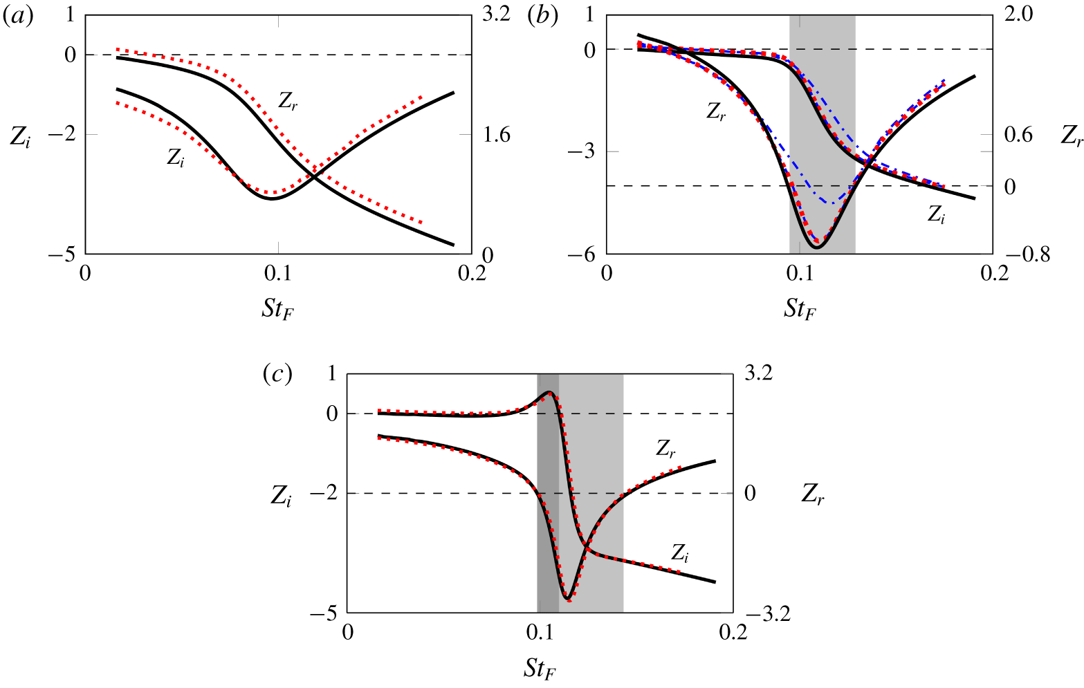
The results for the linear forced case, described in the following, are treated in terms of the real and imaginary parts of the impedance $Z(\unicode[STIX]{x1D714}_{F})$ as a function of the prescribed oscillation frequency represented by the Strouhal number $St_{F}=\unicode[STIX]{x1D714}_{F}D/(2\unicode[STIX]{x03C0}U_{\infty })$ (see figure 2). For validation the linear forced results are compared to fully nonlinear direct numerical simulations (DNS) performed using a spectral-element code. This method is described in detail in Karniadakis & Sherwin (Reference Karniadakis and Sherwin2005), and the implementation used here follows that described in Thompson, Hourigan & Sheridan (Reference Thompson, Hourigan and Sheridan1996). Previous studies using this code for oscillating and coupled vibrating cylinders include Leontini et al. (Reference Leontini, Stewart, Thompson and Hourigan2006a), Leontini, Thompson & Hourigan (Reference Leontini, Thompson and Hourigan2006b) and Leontini et al. (Reference Leontini, Griffith, Lo Jacono and Sheridan2018).

Figure 2.

Components of the impedance as a function of the imposed oscillation frequency for (a) $Re=15$, (b) $Re=25$ and (c) $Re=35$. Linear forced results are shown with a solid black line (——), as well as DNS results for $|\unicode[STIX]{x1D701}_{F}|=0.2$ (dotted-dashed blue line - $\cdot$ - $\cdot$ -), $|\unicode[STIX]{x1D701}_{F}|=0.02$ (dashed blue line – – –) and $|\unicode[STIX]{x1D701}_{F}|=0.002$ (dotted red line $\cdots \cdots$). The convergence of the DNS results to the linear results with decreasing amplitude is clear for the $Re=25$ case shown in (b). The light and dark grey zones represent the first and second instability zones, respectively, according to the Nyquist arguments.

The main parameter that dictates the validity of the comparison between the linear and nonlinear results is the amplitude of the imposed oscillation, which must be small enough to respect the linear hypothesis. The comparison between different imposed amplitudes for the same range of $St_{F}$ at $Re=25$ is presented in figure 2(b), for $Z_{r}(\unicode[STIX]{x1D714}_{F})$ and $Z_{i}(\unicode[STIX]{x1D714}_{F})$. As the amplitude decreases, the DNS solution approaches the linear solution. The results for the two smaller amplitudes give almost the same results, confirming that the considered displacement amplitude is small enough. Another two DNS simulations were carried out at $Re=15$ and $Re=35$ for $|\unicode[STIX]{x1D701}_{F}|=0.002$. Further, one can see from the plotted data that as $Re$ increases, the DNS results tend to more accurately match the linear forced results.

5.2 Instability thresholds established using linear forced oscillations

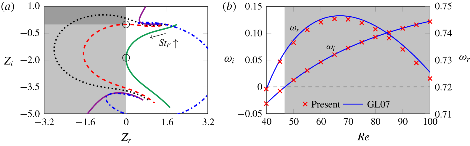
A presentation of the main results for the linear forced case can be seen in figures 2 and 3(a). The latter sketches the results in a Nyquist diagram ($Z_{r}$ versus $Z_{i}$). Two instability zones are highlighted and discussed in the following paragraphs.

Figure 3.

(a) A Nyquist diagram plotting the real and imaginary components of the impedance for the forced results. Each curve represents a constant $Re$, $St_{F}$ progresses along the curve. Values of $Re$ are: $Re=19.915=Re_{c1}$ (solid green line ——); $Re=30.349=Re_{c2}$ (dashed red line - - - - -); $Re=35$ (dotted black line - - - - -); $Re=46.766=Re_{c3}$ (solid violet line ——); $Re=55$ (dotted-dashed blue line - $\cdot$ - $\cdot$ -). The light and dark grey zones represent the first and second instability zones, respectively. (b) A comparison of the eigenvalues calculated from the coupled case for the fluid mode (FM) for $U^{\ast }\rightarrow 0$ at $m^{\ast }=1000$, and those from the fixed-case cylinder (from Giannetti & Luchini (Reference Giannetti and Luchini2007) noted GL07). The grey zone represents the unstable region.

The first interesting phenomenon occurs at $Re=Re_{c1}=19.915$ (shown with the solid green curve, figure 3a) where the sign of $Z_{r}$ first becomes negative at $St_{F,c1}=0.104$, indicating a positive energy transfer from the fluid to the cylinder. The limit condition can be written as

(5.1)$$\begin{eqnarray}\text{At }Re=Re_{c1},\quad \exists \,St_{F}\in \mathbb{R}^{+}\mid Z_{r}(St_{F})=0,\end{eqnarray}$$

and this is represented on the plot as the lighter grey region.

The second interesting phenomenon occurs at $Re=Re_{c2}=30.349$ (shown with the dashed red curve, figure 3a) with the curve that passes exactly through the origin of the Nyquist diagram, indicating that a forcing frequency exists where the impedance is exactly zero. The limit condition for this point can be written as

(5.2)$$\begin{eqnarray}\text{At }Re=Re_{c2},\quad \exists \,St_{F}\in \mathbb{R}^{+}\mid Z(St_{F})=0,\end{eqnarray}$$

and the region where simultaneously $Z_{r}$ is negative and $Z_{i}$ is positive is represented by the darker grey region. The classical Nyquist criterion then states that this value of $Re_{c2}$ presents a lower bound for values of $Re$ that can produce a positive value of $Z_{i}$ – for values of $Re$ beyond this, the Nyquist curve will encircle the origin in an anticlockwise direction. An upper bound exists for this behaviour, $Re_{c3}$, which is explained below. Physically, the condition $Z(St_{F})=0$ implies that there exists a solution of the linearised problem in which the value of $C_{y,F}$ is zero and therefore, following equation (3.1), the energy transfer between the forced case cylinder and the flow will also be zero.

The third critical phenomenon occurs at $Re=Re_{c3}=46.766$ (shown with the solid purple curve, figure 3a). At this $Re$ the steady base flow becomes hydrodynamically unstable. This means that perturbations are expected to grow even in the absence of any forcing, i.e. at a certain $St_{F}$ one will have $Z(St_{F})\rightarrow \infty$ and therefore $\hat{\dot{\unicode[STIX]{x1D701}}}\rightarrow 0$. One observes that the curve tends to infinity, with the limit condition written as

(5.3)$$\begin{eqnarray}\text{at }Re=Re_{c3},\quad \exists \,St_{F}\in \mathbb{R}^{+}\mid Z(St_{F})=\infty .\end{eqnarray}$$

For $Re>Re_{c3}$, the flow is predicted to be unsteady, regardless of the frequency and energy transfer characteristics of a small-amplitude harmonic forcing.

So, the results presented in the Nyquist diagram of figure 3(a) can be interpreted as follows. For $Re\geqslant Re_{c1}=19.915$, there is a range of forcing frequencies which results in a positive energy transfer to the cylinder and therefore the flow is predicted to be unstable. For $Re\geqslant Re_{c2}=30.349$, there is a range of forcing frequencies that produce a positive imaginary component of the impedance $Z_{i}$ within the unstable zone $Z_{r}<0$. For $Re>Re_{c3}=46.766$, the flow is unstable regardless of the form of any linear forcing.

6.1 Eigenmode classification and behaviour

As reported in Cossu & Morino (Reference Cossu and Morino2000), Meliga & Chomaz (Reference Meliga and Chomaz2011) and Navrose & Mittal (Reference Mittal2016) (the latter will hereinafter be denoted as NM16), the coupled transverse cylinder motion introduces two complex-conjugate eigenvalues to the physical spectrum and therefore two eigenmodes, referred to as a fluid mode and a structural mode (EM), as proposed in NM16. This is in contrast to the fixed case, where only FM can be found.

The classification of the two modes found in the coupled moving cylinder case is divided according to their nature and relation. This identification is based on the eigenmode characteristics in the limit of very large $m^{\ast }$ since for this case, the flow-induced vertical force becomes very small compared with the structural ones and the fluid–structure interaction drops to negligible levels (Meliga & Chomaz Reference Meliga and Chomaz2011).

On one hand, the real part of the eigenvalue associated with the EM tends to the natural angular frequency of the cylinder system, i.e. $2\unicode[STIX]{x03C0}/U^{\ast }\equiv \unicode[STIX]{x1D714}_{N}$ and the mode behaves similarly to a cylinder oscillating in vacuo. Further, the imaginary part of the eigenvalue tends to zero, matching this latter behaviour.

On the other hand, the eigenvalue associated with the FM tends to the leading eigenvalue computed for the fixed case, i.e. the mode behaves similarly to the modes in the fixed cylinder case.

However, for relatively low $m^{\ast }$ the distinction between FM and EM is not possible, since eigenvalues may coalesce for certain combinations of $(Re,U^{\ast },m^{\ast })$, especially for lower $m^{\ast }$ or when $Re\rightarrow 46.7$. The two leading eigenmodes do not exhibit a clear distinction in terms of their affiliation to being either a FM or a EM. They are therefore referred as coupled modes and, following NM16 nomenclature, they are denoted as fluid-elastic mode 1 (FEM1) and fluid-elastic mode 2 (FEM2). Further at $Re\geqslant Re_{c3}$, for small $U^{\ast }$, the FEM1 resembles to the FM, whereas the FEM2 is similar to the EM. However, for large $U^{\ast }$, the characteristics of FEM1 and FEM2 resemble the EM and the FM, respectively. For $Re\leqslant Re_{c3}$, the inverse reasoning can be applied and can easily be confirmed in the figures of the following sections.

6.2 Validation

The validation of the results is first done by comparing the results with the fixed-case cylinder, a classical case of hydrodynamic instability. For that purpose, results are obtained for $U^{\ast }\!\rightarrow 0$. This asymptotic approach constrains the spring stiffness to large values, $k\rightarrow \infty$ while $m^{\ast }$ remains finite. It is first noted that the real part of the eigenvalue associated with the EM tends to infinity, for all $Re$, as expected for the natural frequency of the structure-only system, $2\unicode[STIX]{x03C0}/U^{\ast }$. These singularity configurations were intensively studied in Fabre, Assemat & Magnaudet (Reference Fabre, Assemat and Magnaudet2011). The attention of the present study is rather focused on the behaviour of the FM. The imaginary and real parts of the eigenvalue associated with the FM show a good agreement when compared with the fixed case results, reported in Giannetti & Luchini (Reference Giannetti and Luchini2007), as shown in figure 3(b).

Figure 4.

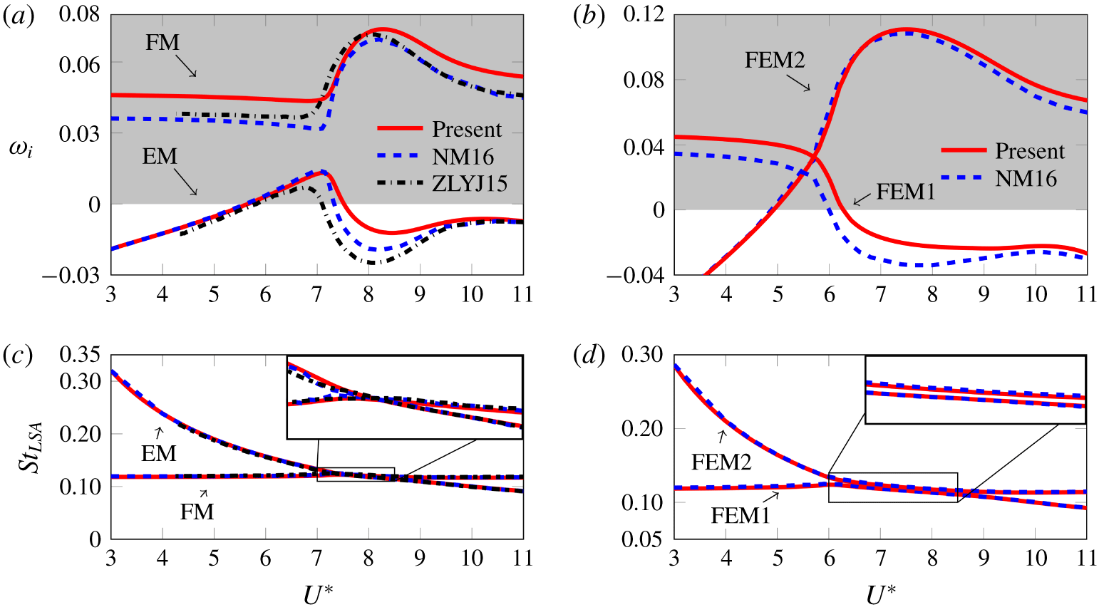
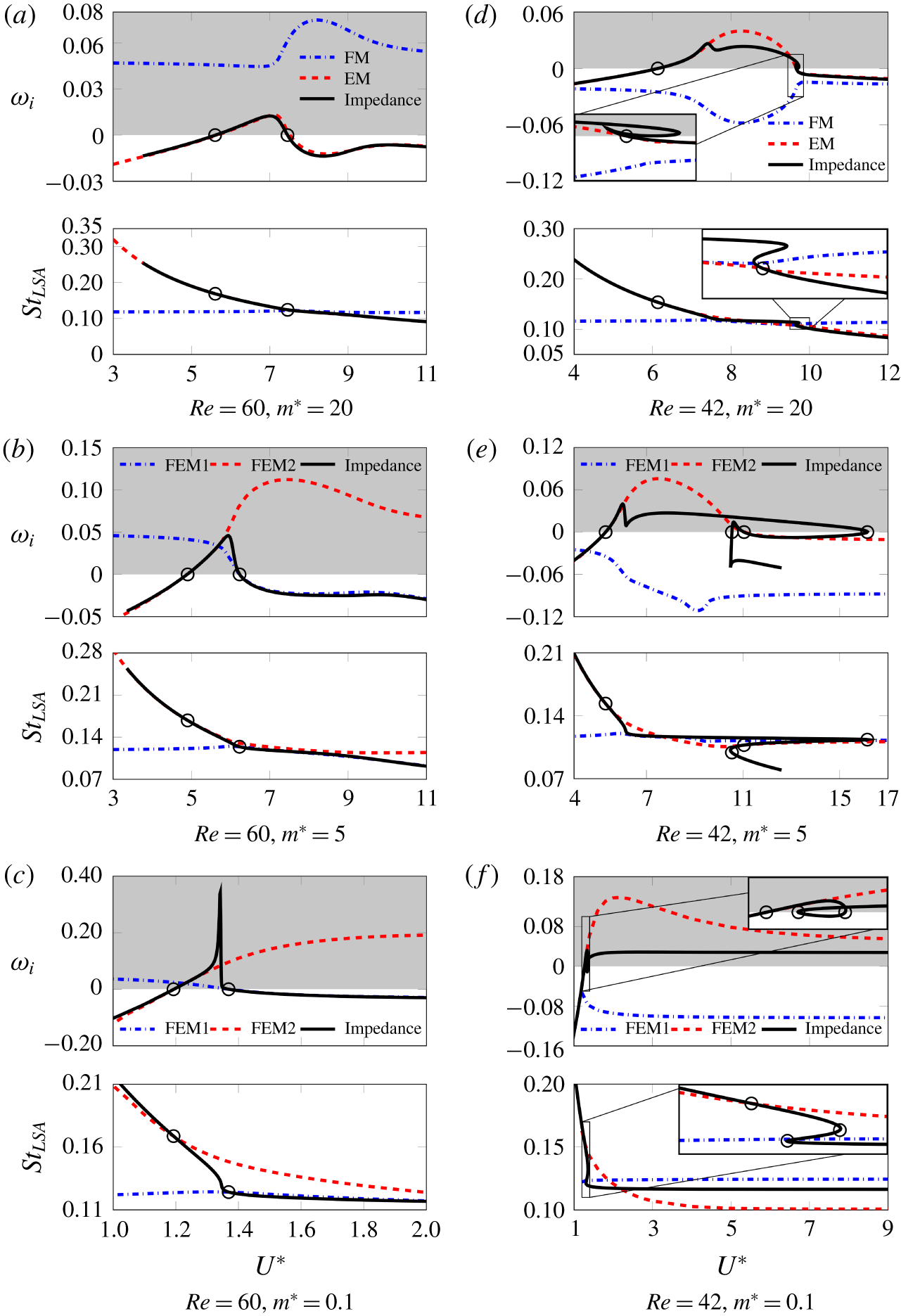
Linear stability results: real and imaginary parts of the eigenvalue $\unicode[STIX]{x1D714}$ with $U^{\ast }$ at $Re=60$ for $m^{\ast }=20$ (a,c) and $m^{\ast }=5$ (b,d). The zoom in the frequency plots ($(c)$ and $(d)$) shows that the curves cross each other for $m^{\ast }=20$ but not for $m^{\ast }=5$. The grey zone represents the unstable region.

The results are also compared with data from NM16 and from Zhang et al. (Reference Zhang, Li and Ye2015) (hereinafter denoted as ZLYJ15). Figure 4 shows the real and imaginary parts of the eigenvalue variation as a function of $U^{\ast }=[3,11]$ for $Re=60$ and $m^{\ast }=\{5,20\}$. Real parts are sketched in terms of $St_{LSA}=\unicode[STIX]{x1D714}_{r}/2\unicode[STIX]{x03C0}$. One can notice that the $St_{LSA}$ associated with the FM remains nearly constant, similar to the $St_{LSA}$ associated with the fixed case, for all values of $U^{\ast }$. Further, one notes that the growth rate of the most unstable mode is maximum within the $U^{\ast }$ range where the frequencies of the two modes are close to each other. This is observed both in this case as in the following ones in the next sections. While the real part presents no difference when comparing the present study and the cited references, the imaginary part of the eigenvalue shows a discrepancy between all sources. Although there is a qualitative match of the results, their values do not agree. However, the present study shows an $\unicode[STIX]{x1D714}_{i}$ at $U^{\ast }=3$ that is close to the fixed-case cylinder value for the same $Re$, depicted in figure 3(b), although this is not verified by the values from NM16 or ZLYJ15. Further, the present LSA results are compared with the impedance-based predictions in the next section, showing a good agreement where the asymptotic theory is valid.

One of the possible causes associated with these differences could be the computational resolution. On one hand, NM16 used a stabilised finite element method based on streamline-upwind/Petrov–Galerkin (known as SUPG) and pressure-stabilizing/Petrov–Galerkin (known as PSPG) techniques (Navrose & Mittal Reference Mittal2016). On the other hand, ZLYJ15 used a reduced-order model of the unsteady Navier–Stokes equations in a finite-volume formulation coupled with the structural motion equations. Both methods differ from that implemented here and could be the cause of the discrepancy. Since the influence of the mesh refinement, boundary conditions and domain size was already explored in the present investigation (see Fabre et al. Reference Fabre, Citro, Ferreira Sabino, Bonnefis, Sierra, Giannetti and Pigou2018), the latter does not seem to be the source of error.

It is clear that, for $Re=60$, an eigenvalue for which $\unicode[STIX]{x1D714}_{i}$ is positive will always exist at any reduced velocity. For the purpose of identifying the stable and unstable zones, a different analysis was carried out at lower $Re$ values which is explored in §§ 6.4 and 6.5.

6.3 Comparison with impedance-based asymptotic predictions

The eigenvalues computed by resolution of the coupled eigenvalue problem are compared with the asymptotic predictions of § 3.2 in figure 5. Figure 5(a) considers the case $Re=60$, $m^{\ast }=20$. In this case, already considered in figure 4(a,c), the FM and the EM are distinct, and the asymptotic prediction accurately follows the eigenvalue of the EM. For $Re=60,m^{\ast }=5$ (figure 5b), a situation close to that in figure 4(b,d) and characterised by coupled modes FEM1 and FEM2, it is observed that the asymptotic prediction first follows the FEM2 branch and then abruptly switches to the FEM1 branch. The same pattern is observed for $Re=60,m^{\ast }=0.1$ (figure 5c), but the asymptotic prediction displays an abrupt behaviour at the transition, which does not fit with the stability results. Still, the prediction correctly reproduces the behaviour in the vicinity of the thresholds.

Figure 5.

Real and imaginary parts of the eigenvalue $\unicode[STIX]{x1D714}$ with $U^{\ast }$ for $Re=60$ (a–c) and $Re=42$ (d–f) for the linear stability analysis of the coupled problem and the impedance-based asymptotic predictions based on the forced problem. The grey zone represents the unstable region.

Consider now the situation for $Re=42$, a value located below the threshold $Re_{c3}\approx 46.7$. In this case, numerical results only provide a single unstable eigenmode (noted EM or FEM2), and a stable mode (noted FM, when corresponding to the fluid, or FEM1). For $m^{\ast }=20$ (figure 5d), the impedance-based prediction asymptotically fits the EM branch around the linearisation value. Note that in this case, the $\unicode[STIX]{x1D714}_{F}-U^{\ast }$ relation defined by (3.9) is multivalued in the range $U^{\ast }\in [9.640-9.729]$. The zoom detail in the figure shows that the asymptotic prediction still correctly fits in the vicinity of the neutral curve but quickly departs from it.

The case $Re=42,m^{\ast }=5$ (figure 5e) is even more complicated. In this case, the asymptotic prediction is multivalued in the range $U^{\ast }\in [10.478-16.147]$ and the corresponding amplification rate crosses the horizontal axis four times (identified with circles in the figure). The results obtained by resolution of the coupled eigenvalue problem are comparatively much simpler, with a single unstable FEM2 branch in the range $U^{\ast }\in [5.304-11.043]$. Note that both these values are correctly predicted by the asymptotic analysis. On the other hand, the thresholds predicted by the asymptotic prediction at $U^{\ast }=10.539$ and $U^{\ast }=16.110$ do not fit with any results. Inspection shows that these values correspond to a change of sign of the real part of the denominator in (3.10), while the numerator $Z_{r}$ is large. Hence, in these ranges the asymptotic prediction is used far away from its starting hypothesis in (3.6), which explains why it does not fit with any physical results.

Finally, for $Re=42,m^{\ast }=0.1$ (figure 5f) the numerically computed branch FEM2 is unstable in the range $U^{\ast }\in [1.270-\infty ]$. Note that in this case there is no upper threshold for restabilisation. The asymptotic prediction displays the same behaviour, but the predictions does not fit at all with stability results for large $U^{\ast }$. Again this range is far from the range of application of the asymptotic theory. Note finally that the asymptotic prediction is multivalued in the range $U^{\ast }=[1.304-1.355]$. The zoom detail in the plot shows that the threshold obtained at $U^{\ast }=1.270$ (which corresponds to a zero of $Z_{r}$) matches with the lower threshold of the stability results, while the two others (which correspond to a change of sign of the real part of the denominator in (3.10)) are incorrect predictions.

6.4 Instability map: $Re{-}U^{\ast }$ plane

The goal of the following section is to identify the stable and unstable zones in the $Re{-}U^{\ast }$ plane, for a fixed mass ratio. By determining the limiting curve where the amplification rate is zero, the region of the parameter space where the cylinder is predicted to vibrate (unstable) can be delineated from the region where the flow is predicted to be steady (stable).

Figure 6.

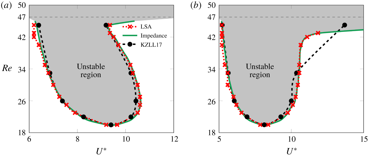
The $Re{-}U^{\ast }$ plane distinguishing the region of instability for (a) $m^{\ast }=50$ and (b) $m^{\ast }=4.73$. Results from the current linear stability analysis, the impedance-based predictions, and the coupled cylinder results of Kou et al. (Reference Kou, Zhanga, Liu and Li2017) (KZLL17).

For this purpose, an LSA was carried out over a wide range of reduced velocity $U^{\ast }$, for several values of $Re$ and at a fixed $m^{\ast }$. The values of $U^{\ast }$ for which $\unicode[STIX]{x1D714}_{i}=0$, for different values of $Re$, for constant values of $m^{\ast }=50$ and $m^{\ast }=4.73$ are first plotted in figures 6(a) and 6(b), respectively. The results are compared with those from Kou et al. (Reference Kou, Zhanga, Liu and Li2017) and the impedance-based predictions at the leading order, observing a very good agreement between results. The unstable zone starts at $Re_{c3}$ for lower $U^{\ast }$ values and tends to a fixed value when $U^{\ast }\rightarrow \infty$. This asymptotic value tends to decrease as $m^{\ast }$ decreases. Therefore, for high values of $m^{\ast }$, the curve will tend to $Re_{c3}$ (figure 6a), whereas for low values of $m^{\ast }$, the curve tends to $Re_{c2}$ (figure 6b).

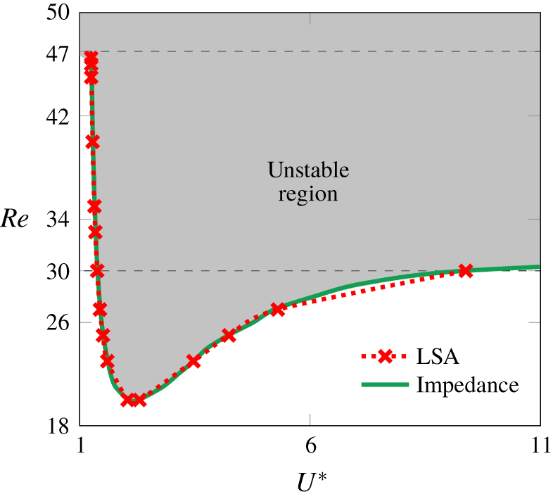
This behaviour is confirmed in figure 7, where the instability threshold is plotted for a very low mass ratio of $m^{\ast }=0.1$. Again, a very close match is observed between the predictions from the linear stability analysis and the impedance-based criterion from the forced case. Also marked on the plot with a dashed line is the value of $Re_{c2}$, which shows that the threshold for instability approaches this value as $U^{\ast }$ increases.

Figure 7.

Stability threshold for $m^{\ast }=0.1$. Compared are the coupled case results using linear stability analysis and the impedance-based predictions. The grey zone represents the unstable region. The dashed line represents the value of $Re_{c2}$, showing that at low $m^{\ast }$ the instability threshold converges to this value as $U^{\ast }$ increases.

This can be explained by considering that for high masses, the oscillation frequency will be similar to the natural structural frequency, and the imaginary component of the impedance $Z_{i}$ will have little effect on the value of $U^{\ast }$ (as shown in (3.9)) and on the growth. Conversely for lower $m^{\ast }$, $Z_{i}$ will impact the dynamics, hence the threshold $Re_{c2}$ where the change of sign of $Z_{i}$ plays a role. A similar reasoning can be used to explain the influence of the damping ratio $\unicode[STIX]{x1D6FE}$ presented below in § 6.6.

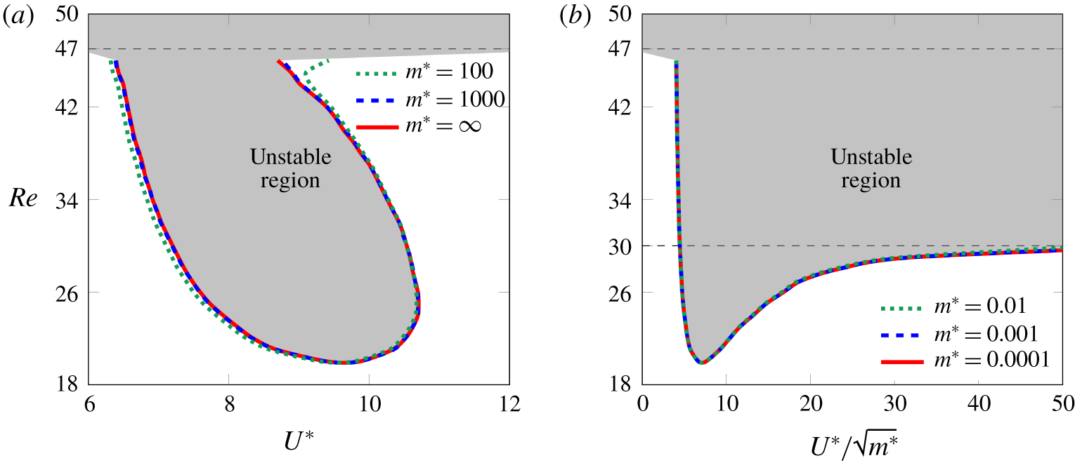
Lastly, the instability threshold curves for the limit cases $m^{\ast }\rightarrow \infty$ and $m^{\ast }\rightarrow 0$ were computed using the impedance arguments at the leading order and are depicted in figure 8. One can see that for high values of mass ratio, the instability threshold curve tends to be the same in the $Re{-}U^{\ast }$ plane (figure 8a). On the other hand, as $m^{\ast }$ tends to zero, a relation in the plane $Re-U^{\ast }/\sqrt{m^{\ast }}$ is found (figure 8b).

Figure 8.

Impedance-based results on the threshold instability curve for (a) the case of $m^{\ast }\rightarrow \infty$ in the $Re{-}U^{\ast }$ plane, and (b) the case of $m^{\ast }\rightarrow 0$ in the $Re-U^{\ast }/\sqrt{m^{\ast }}$ plane. The grey zones represent the unstable regions.

6.5 Instability threshold at $Re\approx 20$

The following analysis is carried out at lower $Re$, fixing $m^{\ast }$ and varying $U^{\ast }$. When decoupled, the eigenvalues associated with the FM always present a negative amplification rate. When coupled, the eigenvalues of one of the modes also obeys this observation (namely the FEM1). The objective is then to determine for which $Re$ the EM (or the other coupled mode, FEM2) presents an eigenvalue with a positive amplification rate and the value of $U^{\ast }$ at which this occurs.

Figure 9.

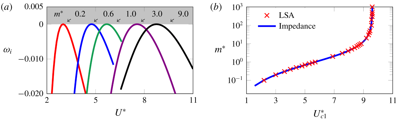
(a) Variation of $\unicode[STIX]{x1D714}_{i}$ with $U^{\ast }$ for different $m^{\ast }$ at $Re_{c1}=19.946$. The value of $m^{\ast }$ is noted above curves in the graphic. The grey zone represents the unstable region. (b) Variation of $U_{c1}^{\ast }$ with $m^{\ast }$ at $Re_{c1}19.946$, comparing the values extracted from the turning points of the curves generated via the linear stability analysis, and the prediction from the impedance from the forced oscillation case.

The first value of $Re$ for which a positive amplification rate $\unicode[STIX]{x1D714}_{i}$ occurs is $Re=Re_{c1}=19.946$. Note that this value is very close to the value of $Re_{c1}=19.915$ predicted via the impedance-based analysis of the linear forced case presented above in § 5.2. Figure 9(a) shows the amplification rate $\unicode[STIX]{x1D714}_{i}$ as a function of $U^{\ast }$ for a series of values of $m^{\ast }$ for a fixed value of $Re=Re_{c1}$. It is clear that regardless of $m^{\ast }$, there is a value of $U^{\ast }$ at the turning point of each curve where the amplification rate is positive and the flow is predicted to be unstable. It is also clear that the value of $U^{\ast }$ – here dubbed $U_{crit}^{\ast }$ – increases with the increase of the mass ratio. The variation of $U_{crit}^{\ast }$ with $m^{\ast }$ is compared in figure 9(b) with the impedance-based predictions as defined in (3.9) – the match is almost perfect. Further, the value of $U_{c1}^{\ast }$ tends to $U_{c1}^{\ast }=9.605$ as $m^{\ast }\rightarrow \infty$, which approaches the value predicted for the natural shedding frequency $f_{N}$ of the fixed cylinder. Indeed, from figure 3(b) one can see that $f_{N}=0.71921/(2\unicode[STIX]{x03C0})=0.1145$ at $Re=40$, which is close to the present critical frequency $f_{c1}^{\ast }=1/9.6048=0.1041$.

6.6 Damping factor effect

To this point, all the discussion has been made by supposing $\unicode[STIX]{x1D6FE}=0$. This assumption intuitively sets the amplification rate of the eigenmodes to their highest values, i.e. for the same set of $(Re,m^{\ast },U^{\ast })$ values, the most linearly unstable mode will be the one with $\unicode[STIX]{x1D6FE}=0$. Any value of $\unicode[STIX]{x1D6FE}$ different from zero will damp the system and render it ‘more stable’.

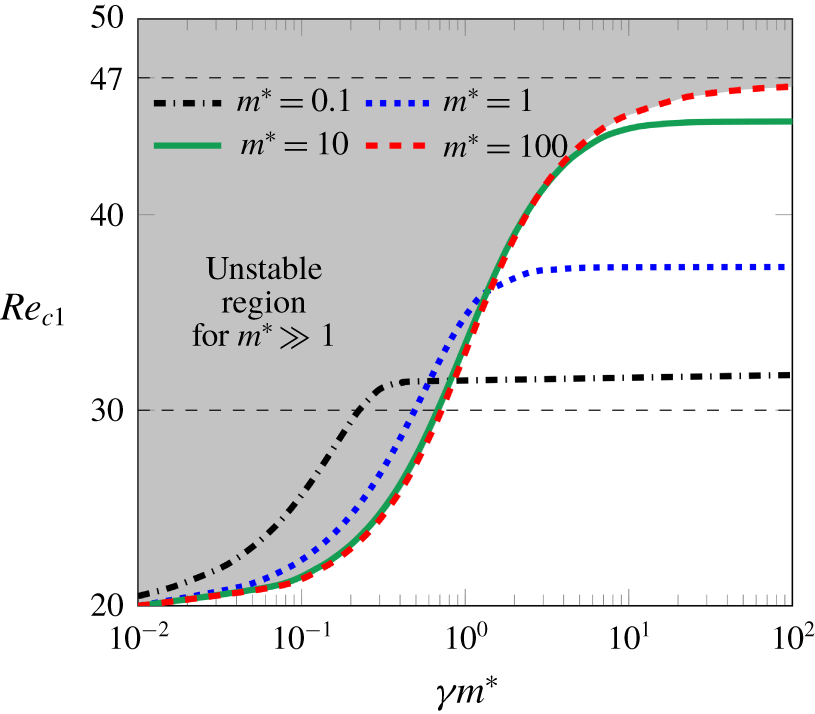
Here this effect is explicitly investigated by examining the effect of the damping factor on the first instability threshold, $Re_{c1}$. A relationship exists between a mass-damping parameter (the product $\unicode[STIX]{x1D6FE}m^{\ast }$) and $Re_{c1}$ for $m^{\ast }\gg 1$. This relation is sketched in figure 10 for several mass ratios. For $\unicode[STIX]{x1D6FE}=0$ (or zero damping), all the curves converge to the $Re_{c1}$ discussed in the previous sections. For high values of $\unicode[STIX]{x1D6FE}$ (or $\unicode[STIX]{x1D6FE}m^{\ast }$), the threshold tends to a different value of $Re$ depending on the mass ratio, in a similar way as shown for increasing $m^{\ast }$ for zero damping as presented in § 6.4. For $m^{\ast }\gg 1$, the threshold tends to the value of the fixed-case cylinder, i.e. $Re_{c1}\rightarrow Re_{c3}$. As the mass ratio decreases, the asymptotic value of $Re_{c1}$ also decreases until it reaches the value of $Re_{c2}$ for $m^{\ast }\ll 1$, i.e.  $Re_{c1}\rightarrow Re_{c2}$. In conclusion, it can be said that the damping removes energy from the system, and hence the instability is only triggered at a higher $Re$.

Figure 10.

The LSA results on the variation of $Re_{c1}$ with the product $\unicode[STIX]{x1D6FE}m^{\ast }$ for several values of $m^{\ast }$. The grey zone represents the unstable region for $m^{\ast }\gg 1$. The horizontal dashed lines indicate the $Re_{c2}$ and $Re_{c3}$.