





1 Introduction
Take two families of dynamical systems; how can we formally compare the dynamical diversity/complexity of the chaotic behavior of each family? In this paper, we study the chaotic components of a system in the framework of local entropy theory, and we use descriptive set theory to formally compare their complexity.
Local entropy theory is a culmination of deep results in combinatorics and topological dynamics. It gives us a way to understand “where” the entropy lies within a system and helps us recognize combinatorially the emergence of entropy using the notion of independence. We refer the reader to the survey articles [Reference Glasner and Ye25, Reference García-Ramos and Li21] and the book by Kerr and Li [Reference Kerr and Li35, Chapter 12] for more information on the subject. It turns out that local entropy theory is a powerful tool that can be applied in a variety of settings. For example, local entropy theory provides a direct and an intuitive reason as to why positive entropy is stronger than Li-Yorke chaos [Reference Blanchard, Glasner, Kolyada and Maass7, Reference Kerr and Li34]. It can also be used to find homoclinic points of algebraic actions [Reference Chung and Li9, Reference Barbieri, García-Ramos and Li2]. In another application of this theory, the first author and Kato [Reference Darji and Kato13] settled some old problems concerning indecomposable continua in dynamical systems.
Local entropy theory was introduced by Blanchard [Reference Blanchard6]. His original motivation was to understand the topological analogues of K-systems, that is, ergodic systems all of whose nontrivial factors have positive entropy. To this end, Blanchard gave two possible interpretations: uniformly positive entropy (UPE) systems and completely positive entropy (CPE) systems. Blanchard realized that both of these conditions can be characterized using a new local concept. Thus was born the notion of entropy pairs and the area of local entropy theory. See [Reference Glasner and Ye25] for a survey on the subject. This theory is useful, not only for understanding positive entropy, but also for understanding zero entropy systems such as null and tame systems. Building on the seminal work of various mathematicians and developing new elegant ideas, Huang and Ye [Reference Huang and Ye30], and Kerr and Li [Reference Kerr and Li34] provided a unified approach to local entropy theory. This unified approach is of combinatorial nature and uses the concept of independence.
In his original article [Reference Blanchard5], Blanchard showed that every topological dynamical system (TDS) that has uniformly positive entropy also has completely positive entropy, but the converse is not true. Using a natural rank called the
$\Gamma $
 -rank, Barbieri and the second author [Reference Barbieri and García-Ramos3] constructed a transfinite hierarchy of families that have completely positive entropy but not uniformly positive entropy. This was the first inkling of the relationship between local entropy theory and descriptive set theory.
Topological dynamics and ergodic theory are sibling branches of dynamical systems in which several notions can be translated from one branch to the other. See surveys [Reference Glasner and Weiss24, Reference Huang, Shao and Ye32] for such connections. For a fixed compact metrizable space X, respectively a probability space X, we can consider the space of all topological dynamical systems, respectively, all measure-preserving systems, on X. Equipped with a suitable natural topology, such collections form Polish spaces. Now we can ask several interesting questions. For example, how big is a subcollection of dynamical systems with a particular property? Or what is its descriptive complexity? In particular, is it Borel?
The study of such questions has a long history. In the context of ergodic theory, we have a result of Halmos of 1944 [Reference Halmos26] which states that among measure-preserving transformations those that are weak-mixing form a residual
$G_{\delta }$
 set. The first “anti-classification” or non-Borel result in dynamics emerged in a paper by Beleznay and Foreman [Reference Beleznay and Foreman4] where they proved that the collection of distal topological dynamical systems is complete coanalytic and hence not Borel.
From the descriptive complexity viewpoint, most of the classical families of measurable chaotic dynamical systems are Borel: mixing [Reference Rohlin38], Bernoulli [Reference Feldman16], positive entropy and K-systems [Reference Foreman18]. In the context of topological dynamics, it is fairly routine to show that families of systems which are weak-mixing, mixing, Bernoulli shifts and have positive entropy are all Borel. Now, as exhibited by Blanchard, K-systems have at least two distinct interpretations in topological dynamics, namely UPE and CPE. It turns out that the class of UPE systems again is Borel, Corollary 3.2. However, it follows from the results of Barbieri and the second author [Reference Barbieri and García-Ramos3], and Westrick [Reference Westrick45], that CPE is not Borel. Informally speaking, this implies that no amount of inherently countable resources can settle the question of whether a TDS has completely positive entropy or not.
There are also some recent results regarding effective (or light face) descriptive set theory, CPE, and symbolic dynamics. The collection of SFTs is a countable set and hence
$F_{\sigma }$
 . Thus, effective descriptive set theory is the appropriate context for determining their complexity. It follows from a result of Pavlov [Reference Pavlov37], that SFTs with zero-dimensional-CPE (factors having dimension zero) is effectively Borel. Meanwhile, Westrick [Reference Westrick45] showed that the family of CPE
$\mathbb {Z}^{2}$
 -subshifts of finite type (SFT) is effectively complete coanalytic. Returning to classical descriptive set theory, Salo [Reference Salo41] constructed CPE subshifts on
${\mathbb Z}$
 that have arbitrarily high entropy rank; this result can be used to show that in the space of all
${\mathbb Z}$
 -subshifts, the class of CPE subshifts forms a non-Borel collection.
In this article, we initiate a systematic study of the relationship between local entropy theory, in particular properties of UPE and CPE, and descriptive complexity. As mentioned earlier, the collection of CPE systems on a Cantor space is coanalytic and not Borel [Reference Barbieri, García-Ramos and Li2], [Reference Westrick45] and this can be further refined by making the maps shift maps [Reference Salo41], [Reference Westrick45]. At this point, two questions arise: does the descriptive complexity change as we vary the underlying phase space and as we require extra conditions on the map?
Our first result is that for a very general class of phase spaces, if the maps are left unrestricted, then the class of CPE systems is a complete coanalytic subset. Recall that all complete coanalytic sets are non-Borel. Below we state it for the interval in
${\mathbb R}^n$
 and in Remark 4.2, we explain how to obtain the result for graphs and orientable manifolds.
Theorem 4.1.
For every
$d\geq 1$
 ,
$\text {CPE}(I^d)$
 is complete coanalytic.
A curious phenomenon occurs when we require the map to have finer properties. A result of Blokh [Reference Blokh8] implies that for the interval and, in general, for every topological graph X, every mixing CPE system is also UPE. As the collection of UPE systems is Borel, we have the following corollary.
Corollary 3.9.
Let X be a topological graph. Then
$\text {Mix}(X)\cap \text {CPE}(X)$
 is Borel.
A similar situation occurs for maps with the shadowing property, that is, on any compact metrizable space, a shadowing system is UPE if and only if it is CPE, Corollary 3.4. As such, we have the following corollary.
Corollary 3.6.
Let X be a compact metrizable space. Then
$\text {Shad}(X)\cap \text {CPE}(X)$
 is Borel.
It may seem that for maps which are of most interest in dynamical systems such as transitive, mixing, chaotic, etc., the property of having CPE is Borel. The main result of this article is to show that this is false. Namely, the following holds.
Theorem 5.25.
Let X be a Cantor space. Then,
$\text {Mix}(X) \cap \text {CPE}(X)$
 is coanalytic and not Borel.
The proof of Theorem 4.1 is short and somewhat easy to verify once the main idea is stated. On the other hand, the proof of Theorem 5.25 is rather delicate and involved, as evident in Section 5.1. It is not surprising that proving that a family of dynamical systems is not Borel is technically difficult for transitive and mixing maps. Usually, the easiest path to proving that a family of nonreducible systems, for example, nonergodic or nontransitive, is not Borel, is to build examples with countably many components as done in [Reference Barbieri and García-Ramos3] and in Section 3. This is analogous to what happened for the conjugacy problem in ergodic theory. First, Hjorth proved that the equivalence relation generated by the conjugacy of measure-preserving transformations is not Borel [Reference Hjorth28]. Later, Foreman, Rudolph, and Weiss [Reference Foreman, Rudolph and Weiss19], using a much more delicate construction, proved the same for ergodic systems.
The paper is organized as follows. In Section 2 we give a somewhat detailed introduction to local entropy theory and descriptive set theory so that the article is accessible. In Section 3 we investigate the relationship between shadowing and local entropy. In Section 4 we study the complexity of CPE systems on topological manifolds. In Section 5 we prove the main result of the paper. Several open questions arise from the above, which will be discussed in Section 6.
2 Preliminaries
In this section, we will give the basic definitions needed for the paper, as well as an introduction to local entropy theory and descriptive set theory for nonexperts.
Let Z be a set and
$F\subseteq Z^2$
 . We define the transitive closure of F as follows

A set
$F\subseteq Z^{2}$
 is an equivalence relation if and only if F is symmetric,
$\Delta _{Z}\subseteq F$
 , and
$F=F^{+}$
 . In this case, we denote the equivalence class of
$z\in Z$
 by
$[z]_{F}$
 .
Throughout this paper, X is always a compact metrizable space with a compatible metric d.
Let
$E\subseteq X^{2}$
 be a symmetric set. We define

For an ordinal
$\alpha $
 ,
$\Gamma ^{\alpha }(E)$
 is defined by

if
$\alpha $
 is the successor ordinal and

if
$\alpha $
 is a limit ordinal.
As every compact metric space has a countable basis, every strictly increasing transfinite sequence of closed sets must be countable.
From this we have the following.
Proposition 2.1. Let X be a compact metrizable space and
$E\subseteq X^2$
 symmetric. There exists a countable ordinal
$\alpha $
 such that
$\Gamma ^{\alpha } (E)=\Gamma ^{\alpha +1}(E)$
 .
The smallest such ordinal is called the
$\Gamma $
 -rank of E. We define
$\Gamma ^{\infty } (E)=\Gamma ^{\alpha } (E)$
 , where
$\alpha $
 is the rank of E.
The Cantor set
$C\subseteq [0,1]$
 is the standard Cantor ternary set. A Cantor space is a nonempty compact metrizable space that is totally disconnected (i.e., the only connected subsets are singletons) and has no isolated points. Every Cantor space is homeomorphic to the Cantor set [Reference Willard46, Corollary 30.4].
2.1 Topological dynamics and local entropy theory
We say that
$(X,T)$
 is a topological dynamical system (TDS) if X is a compact metrizable space and
$T:X\rightarrow X$
 is a continuous function. A TDS is (topologically) mixing if for every pair of nonempty open sets
$U,V$
 there exists
$N>0$
 such that
$T^{-n}(U)\cap V\neq \emptyset $
 for every
$n\geq N$
 . We say
$(X_2,T_2)$
 is a factor of
$(X_1,T_1)$
 if there exists a surjective continuous function
$\phi : X_1\rightarrow X_2$
 (called a factor map) such that
$\varphi \circ T_{1}=T_{2}\circ \varphi $
 . It is well-known that all factors of mixing TDSs and all countable products of mixing TDSs are mixing.
Let
$(X,T)$
 be a TDS and
$\mathcal {U},\mathcal {V}$
 open covers of X. We denote the smallest cardinality of a subcover of
$\mathcal {U}$
 by
$N(\mathcal {U})$
 , and

We define the entropy of
$\mathbf {(X,T)}$
 with respect to
$\mathbf {\mathcal {U}}$
 as

The (topological) entropy of
$(X,T)$
 is defined as

In order for a TDS to have positive entropy it is only necessary for a small portion of the system to be chaotic. In a broad sense, local entropy theory tackles the following questions: where can we localize the entropy of a given system? how can we define a system that has entropy everywhere?
For measure-preserving systems, the idea of entropy “everywhere” goes back to Kolmogorov. A measure-preserving system is a K-system if it satisfies Kolmogorov’s zero-one law. The Rohlin-Sinai theorem states that a measure-preserving system is a K-system if and only if every nontrivial (measurable) factor has positive (measurable) entropy if and only if the system has positive (measurable) entropy with respect to any nontrivial (measurable) partition [Reference Glasner22, Theorem 18.9]. In dynamical systems, one often studies analogous properties in topological and measurable contexts [Reference Glasner and Weiss24, Reference Huang, Shao and Ye32]. In [Reference Blanchard5], two possible topological analogues of the K-systems were introduced.
Definition 2.2. A TDS has completely positive entropy (CPE) if every nontrivial factor has positive entropy. In this case, we call this a completely positive entropy system or simply CPE system.
A TDS has uniformly positive entropy if for every open cover
$\mathcal {U}$
 consisting of nondense sets, we have
$h_{\text {top}}(X,T,\mathcal {U})>0$
 . In this case, we call this a uniformly positive entropy system or simply UPE system.
It turns out that these two notions are not equivalent. Every UPE system is a CPE system, but the converse does not hold. A UPE system is not necessarily mixing, but it is always weak-mixing [Reference Blanchard5]. On the other hand, there exist CPE systems that are not transitive.
The question “where can we localize the entropy?” has to do with how points relate to each other through dynamics. Hence, this question is not answered in X but in
$X^2$
 . Informally, a pair is an entropy pair if every cover that separates the points has positive entropy. In this paper, we will not give the original definition of Blanchard. Instead we will use the equivalent definition of IE-pairs (independence entropy pairs). The concept of independence (or interpolation) on dynamical systems appeared in the work of Glasner and Weiss [Reference Glasner and Weiss23] based on ideas of Rosenthal [Reference Rosenthal39], and Huang and Ye [Reference Huang and Ye29, Reference Huang and Ye30]. We will follow the definition of independence entropy pairs of Kerr and Li [Reference Kerr and Li34].
Given a TDS
$(X,T)$
 and
$\{U,V\}\subseteq X$
 , we say
$I \subseteq \mathbb {N}$
 is an independence set for
$\mathbf {\{U,V\}}$
 if for all finite
$J \subseteq I$
 , and for all
$(Y_j) \in \prod _{j\in J}\{U,V\}$
 , we have

A set
$I \subseteq \mathbb {N}$
 has positive density if the following limit exists
$\lim _{n \rightarrow \infty } \frac {|I \cap [1,n]|}{n}>0$
 .
Definition 2.3. Let
$(X,T)$
 be a TDS. We say that
$(x_1, x_2) \in X\times X$
 is an independence entropy pair (IE-pair) of
$\mathbf {(X,T)}$
 if for every pair of open sets
$A_1,A_2$
 , with
$x_1\in A_1$
 and
$x_2\in A_2$
 , there exists an independence set for
$\{A_1, A_2\}$
 with positive density. The set of IE-pairs of
$(X,T)$
 will be denoted by
$E(X,T)$
 .
We have
$E(X,T)\subseteq X^2$
 is a closed subset [Reference Kerr and Li34, Proposition 3.9]. For the proof of the following results, see [Reference Kerr and Li35, Theorem 12.19] and [Reference Huang, Ye and Zhang31].
Theorem 2.4. Let
$(X_1,T_1)$
 and
$(X_{2},T_{2})$
 be TDSs.
-
1. $(X_1,T_1)$
 , has positive entropy if and only if there exists
$x\neq y\in X_1$
with
$(x,y)\in E(X_1,T_1)$
.
-
2. $E(X_1\times X_{2},T_1\times T_{2})=E(X_1,T_1)\times E(X_{2},T_{2})$
. -
3. Let $\phi :X_1\rightarrow X_2$
be a factor map. Then
$E(X_2,T_2)=(\phi \times \phi )(E(X_1,T_1))$
. -
4. $(X_1,T_1)$
and
$(X_{2},T_{2})$
have CPE if and only if
$(X_1\times X_{2},T_1\times T_{2})$
has CPE.






Now we will study the
$\Gamma $
 -rank defined at the beginning of this section in the particular case when
$E=E(X,T)$
 is the set of independence entropy pairs.
Definition 2.5. Let
$(X,T)$
 be a TDS. The entropy rank of
$(X,T)$
 is the
$\Gamma $
 -rank of
$E(X,T)$
 .
Entropy pairs can be used to characterize CPE and UPE. An equivalent statement of the following results was proved in [Reference Blanchard6] (also see [Reference Kerr and Li35, Theorem 12.30]).
Theorem 2.6. A TDS has completely positive entropy if and only if
$\Gamma ^{\alpha }(E(X,T))=X^{2}$
 where
$\alpha $
 is the entropy rank of
$(X,T)$
 .
Proposition 2.7. A TDS has uniformly positive entropy if and only if
$E(X,T)=X^2$
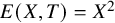 .
That is, a TDS has UPE if and only if it has CPE and entropy rank 0. In fact, if
$(X,T)$
 has CPE then
$\Delta _X\subseteq E(X,T)$
 so in this case to prove entropy rank 0, we only need to show that
$E(X,T)=E(X,T)^+$
 .
Given a compact metrizable space X, we define
$\text {TDS}(X)$
 as the set of all continuous functions from X into X endowed with the uniform topology generated by the sup metric.
Note that
$\text {TDS}(X)$
 is a Polish space. We also define the following subspaces


Although they are clearly related, we will stress the formal differences of talking about CPE and UPE as properties of dynamical systems and
$\text {CPE}(X)$
 and
$ \text {UPE}(X)$
 as Polish spaces.
2.2 Descriptive set theory
Descriptive set theory and dynamical systems have a longstanding relationship. A few years after Halmos proved that the collection of weak-mixing measure-preserving systems is a dense
$G_{\delta }$
 set [Reference Halmos26, Reference Halmos27], Rohlin proved that the collection of mixing measure-preserving systems is meager. While not constructive, this provided the first proof that there exist weak-mixing but nonmixing measure-preserving systems. Descriptive set theory can also be used to prove anti-classification results. This is done by proving that a certain property or equivalence relation cannot be characterized using countable resources.
In this section, we recall the basics of classical descriptive set theory. We refer the reader to [Reference Kechris33] for more details.
Let
$\mathcal {X}$
 be a Polish space (separable completely metrizable topological space). A subset of
$\mathcal {X}$
 is Borel if it belongs to the smallest
$\sigma $
 -algebra generated by the open sets. Borel sets naturally fall into the Borel hierarchy:

where
$\Sigma ^0_1$
 is the collection of all open sets,
$\Pi ^0_{\alpha }$
 is the collection of sets whose complement is in
$\Sigma ^0_{\alpha }$
 and
$\Sigma ^0_{\alpha }$
 is the collection of countable unions of sets from
$\Pi ^0_{\beta }$
 ,
$\beta < \alpha $
 . Moreover,
$\Sigma ^0_{\beta }\cup \Pi ^0_{\beta } \subseteq \Sigma ^0_{\alpha }\cap \Pi ^0_{\alpha }$
 whenever
$\beta < \alpha $
 , that is, the hierarchy is increasing. If
$\mathcal {X}$
 is uncountable, then the hierarchy is strictly increasing, that is, there are sets that belong to the
$\alpha $
 levels but not the previous ones.
Beyond the Borel hierarchy sits the projective hierarchy. We are particularly interested in the first level of the projective hierarchy, that is, analytic and coanalytic sets. We say that a subset of a Polish space is analytic if it is the continuous image of a Borel subset of a Polish space and coanalytic (or, equivalently,
$\Pi _1^1$
 ) if it is the complement of an analytic set. All Borel subsets of a Polish space are both analytic and coanalytic. Moreover, if a set is both analytic and coanalytic, then it must be Borel. However, in every uncountable Polish space there are analytic, and hence coanalytic, sets that are not Borel. Loosely speaking, if a set is analytic or coanalytic but not Borel, it cannot be described with countably many quantifiers over a countable set.
A standard method to prove a coanalytic set is not Borel is to reduce it to a known combinatorial set which is not Borel. More specifically, if
$\mathcal {B}$
 is a known non-Borel subset of some Polish
$\mathcal {Y}$
 ,
$\mathcal {A} \subseteq \mathcal {X}$
 and
$f:\mathcal {Y}\rightarrow \mathcal {X}$
 is a Borel function such that
$f^{-1}( \mathcal {A}) = \mathcal {B}$
 , then
$\mathcal {A}$
 is not Borel. In this case, we say that
$\mathcal {B}$
 is Borel reducible to
$\mathcal {A}$
 . This inspires the following definition.
Definition 2.8. A coanalytic set
$\mathcal {A}$
 of a Polish space
$\mathcal {X}$
 is complete coanalytic (or
$\Pi _1^1$
 -complete) if for every coanalytic set
$\mathcal {B}$
 of a Polish space
$\mathcal {Y}$
 there exists a Borel function
$f:\mathcal {Y}\rightarrow \mathcal {X}$
 such that
$f^{-1}( \mathcal {A}) = \mathcal {B}$
 .
In some sense complete coanalytic sets are as complicated as coanalytic sets can be. The following proposition simply follows from the definition and the fact that the composition of Borel functions is Borel.
Proposition 2.9. Let
$\mathcal {A}$
 be a coanalytic subset of a Polish space
$\mathcal {X}$
 and
$\mathcal {B}$
 be a complete coanalytic subset of a Polish space
$\mathcal {Y}$
 . If there exists a Borel function
$f:\mathcal {Y}\rightarrow \mathcal {X}$
 such that
$f^{-1}( \mathcal {A}) = \mathcal {B}$
 , that is,
$\mathcal {B}$
 is Borel reducible to
$\mathcal {A}$
 , then
$\mathcal {A}$
 is also complete coanalytic.
A classical combinatorial example of a complete coanalytic set is WF, the set of all well-founded trees on
$\mathbb {N}$
 ; see [Reference Kechris33, p.243]. In practice, one normally Borel reduces WF to a given coanalytic set to show that the given coanalytic set is complete coanalytic. In our case, we will use a result of Hurewicz to obtain a combinatorial complete coanalytic set, that is, the set of all countable compact subsets of a Cantor space is complete coanalytic [Reference Kechris33, p. 245]. In particular, in Theorem 4.1, we will reduce this set of Hurewicz to prove that
$\text {CPE}([0,1]^d)$
 is
$\Pi ^1_1$
 -complete.
An alternate method for proving that a coanalytic set is not Borel is to use the so-called “rank method.” Often coanalytic sets in natural settings admit a natural rank, that is, an assignment which associates a countable ordinal to each element. If this assignment is a
$\Pi ^1_1$
 -rank and the rank is unbounded, then the set in question is not Borel. More precisely, we have the following definition.
Definition 2.10. Let
${\mathcal X}$
 be a Polish space,
${\mathcal C} \subseteq {\mathcal X}$
 and
$\varphi : {\mathcal C} \rightarrow \omega _1$
 . We say that
$\varphi $
 is a
$\boldsymbol {\Pi ^1_1}$
 -rank if
${\mathcal C}$
 is
$\Pi ^1_1$
 and there are relations
${\mathcal P}, {\mathcal Q} \subseteq {\mathcal X}^2$
 , one of them
$\Sigma ^1_1$
 and the other
$\Pi ^1_1$
 , such that for all
$y \in {\mathcal C}$
 we have

Loosely speaking,
$\varphi $
 is a
$\Pi ^1_1$
 -rank if
$\{x: \varphi (x) \le \varphi (y)\} $
 is “uniformly Borel in y.”
Theorem 2.11 [Reference Kechris33, Section 35.E].
Let
${\mathcal C}$
 be a
$\Pi ^1_1$
 set and
$\varphi $
 be a
$\Pi ^1_1$
 -rank on
${\mathcal C} $
 . If
${\mathcal A} \subseteq {\mathcal C}$
 is
$\Sigma ^1_1$
 , then
$\varphi $
 is bounded on
${\mathcal A} $
 , that is, there exists
$\alpha < \omega _1$
 such that
$\varphi (x) < \alpha $
 for all
$x \in {\mathcal A} $
 . In particular,

A classical
$\Pi ^1_1$
 -rank known as the Cantor-Bendixson rank will be useful to us. Given a compact set A, we let
$A'$
 denote the Cantor-Bendixson derivative of A, that is, the set of all limit points of A. For countable ordinal
$\alpha $
 ,
$A^{\alpha }$
 , the
$\alpha {th}$
 Cantor-Bendixson derivative of A, is defined by transfinite recursion as follows


Of course, from separability we have that for each compact set A there is a countable ordinal
$\alpha $
 such that
$A^{\alpha } = A^{\alpha +1}$
 . The least such
$\alpha $
 is called the Cantor-Bendixson rank of A
and is denoted by
$|A|_{CB}$
 . Moreover, we define
$A^{\infty } = A^{|A|_{CB}}$
 . For a fixed compact metrizable space X, the set of all countable compact subsets of X is a
$\Pi ^1_1$
 set and the Cantor-Bendixson rank is a
$\Pi ^1_1$
 -rank on this set [Reference Kechris33, Section 6].
Returning to our particular case of
$\text {CPE}(X)$
 , the following results will allow us to use the rank method. The first result is probably known but we include it for the sake of completeness.
We work with a fixed Hilbert cube
$\mathbf {H}$
 . We will assume that all our spaces are subsets of
$\mathbf {H}$
 . As every compact metric space is homeomorphic to a subset of
$\mathbf {H}$
 ,
$T:X \rightarrow X$
 being CPE is equivalent to saying that T has no nontrivial factor whose phase space is a subset of
$\mathbf {H}$
 . We denote the surjective continuous functions from X to
$X'$
 by
$C_s(X,X')$
 .
We define

We equip
$\mathbf {P}$
 with the Hausdorff metric
$\textbf {d}_H((T_1,T_1',f_1),(T_2,T_2',f_2))$
 when considered as a subset of
$(\mathbf {H}^2)^3$
 . We set the following space of factor systems

and the space of nontrivial factor systems as

Let
$\mathbf {H}$
 be the Hilbert cube, and
$X,X'$
 compact metrizable spaces. We denote by
$\mathbf {X}\subset \mathbf {H}$
 the subset so that X and
$\mathbf {X}$
 are homeomorphic. For every
$T\in \text {TDS}(X)$
 we denote by
$\mathbf {T}\subset \mathbf {X}^2$
 the associated continuous function so that
$(X,T)$
 is conjugated to
$(\mathbf {X},\mathbf {T})$
 . We denote the surjective continuous functions from X to
$X'$
 by
$C_s(X,X')$
 . For every
$f\in C_s(X,X')$
 we denote by
$\mathbf {f}\subset \mathbf {X}\times \mathbf {X'}$
 the associated function.
We define

We equip
$\mathbf {P}$
 with the metric
$\textbf {d}((T_1,T_1',f_1),(T_2,T_2',f_2))=d_H((\mathbf {T_1},\mathbf {T_1'},\mathbf {f_1}),(\mathbf {T_2},\mathbf {T_2'},\mathbf {f_2}))$
 , where
$d_H$
 is the Hausdorff metric on
$(\mathbf {H}^2)^3$
 . We set the following space of factor systems

and the space of nontrivial factor systems as

Lemma 2.12. We have
$\mathbf {P}$
 is a Polish space and
$\mathbf {F},\mathbf {F'}$
 are Borel subsets of
$\mathbf {P}$
 .
Proposition 2.13. Let X be a compact metrizable space. Then,
$\text {CPE}(X)$
 is coanalytic.
Proof. Vetokhin showed [Reference Vetokhin43] that the assignment which takes a TDS to its entropy is Borel (in fact, of Baire class two). This implies that

is Borel. By the definition, we have a TDS has CPE if and only if all its nontrivial factors have positive entropy. As CPE is characterized by the quantifier
$\forall $
 on a Borel condition, we obtain that
$\text {CPE}(X)$
 is coanalytic.
The following result was proved in the context of effective descriptive set theory [Reference Westrick45, Corollary 2]. Using a notion of Borel expansion we give an alternate classical descriptive set-theoretic proof in [Reference Darji and García-Ramos12].
Theorem 2.14. Let X be a compact metrizable space. The entropy rank is a
$\Pi ^1_1$
 -rank on
$\text {CPE}(X)$
 .
Examples of TDSs of arbitrarily high entropy rank have been found for Cantor maps [Reference Barbieri and García-Ramos3] and subshifts [Reference Salo41]. These examples are not transitive (let alone mixing). By applying the rank method to the coanalytic set,
$\text {Mix}(X) \cap \text {CPE}(X)$
 (X being a Cantor space), we will see in Theorem 5.25 that it is not Borel.
3 When CPE and UPE are equivalent
In this section, we show that
$\text {UPE}(X)$
 is a Borel space and we will explain how in some situations CPE and UPE are equivalent properties. As mentioned earlier, any UPE system is also CPE. We show that any CPE system with the shadowing property is also UPE. It is known that for graph maps, the properties of being mixing and having UPE are equivalent [Reference Ruette40, Page 107]. Hence, for mixing graph maps, we also have that having CPE and having UPE coincide.
The fact that the class of UPE systems is Borel can be proved using rank theory, that is, the collection of objects whose rank is bounded under a
$\Pi ^1_1$
 -rank forms a Borel set. We give an alternative proof which may be useful in determining the exact descriptive complexity of the class of maps that have UPE on a given space. In this paper we will not study the complexity of Borel sets, but we note that Borel complexity has been studied in dynamical contexts in [Reference Clemens10, Reference Gao, Jackson and Seward20, Reference Airey, Jackson, Kwietniak and Mance1].
We denote by
$K(X)$
 , the collection of nonempty compact subsets of X endowed with the Hausdorff metric. For a definition of the Hausdorff metric see [Reference Engelking14, Section 4.5.23]. Note that if X is compact then so is
$K(X)$
 . Let
$\mathcal {U}=\{U_{1},\ldots ,U_{n}\}$
 be a collection of nonempty open sets of X. We define

We have
$\{A_{\mathcal {U}}\}_{\mathcal {U}}$
 , where
$\mathcal {U}$
 runs over all finite collections of nonempty open subsets of X, forms a basis for the topology on
$K(X)$
 induced by the Hausdorff metric.
Proposition 3.1. Let X be a compact metrizable space and let

be given by
$E(T) = E(X,T)$
 . Then, E is a Borel map.
Proof. Let
$U,V$
 be nonempty open in X. We will first observe that

is Borel. Indeed, using an equivalent definition of independence given in [Reference Kerr and Li34, Lemma 3.2] we have that
$\dagger $
 is satisfied by T if and only if there is a rational number
$ r>0 $
 such that for all
$l \in \mathbb {N}$
 there is an interval
$I \subseteq \mathbb {N}$
 with
$|I| \ge l$
 and a finite set
$F \subseteq I$
 with
$|F| \ge r |I|$
 such that F is an independent set for
$(U,V)$
 . It is easy to verify that for fixed
$U,V, r, l, I, F$
 set

is open. Now the set in
$\dagger $
 is the result of a sequence of countable unions and countable intersections of sets of type
$\ddagger $
 . Hence
$\dagger $
 is Borel. Since X has a countable basis, by taking unions, we have that
$\dagger $
 is Borel when
$U \times V$
 is replaced by any open set
$W \subseteq X \times X$
 . Every closed set in
$X \times X$
 is the monotonic intersection of a sequence of open sets in
$X \times X$
 . This and the fact that
$E(T)$
 is closed imply that
$\dagger $
 is Borel when
$U \times V$
 is replaced by a closed set
$C \subseteq X \times X$
 . Reformulating the last statement, we have for all open
$W \in X \times X$
 , the set

is Borel. Putting
$\dagger $
 and
$\diamond $
 together, we have

is Borel whenever
$W_1, \ldots ,W_n$
 are open in
$X^2$
 , completing the proof.
Now applying Proposition 2.7, we obtain the following.
Corollary 3.2. Let X be a compact metrizable space. we have
$\text {UPE}(X)$
 is Borel.
Let
$(X,T)$
 be a TDS and
$\delta>0$
 . We say
$\left \{ x_{n}\right \} _{n\in \mathbb {N}}\subseteq X$
 is a
$\delta $
 -pseudo-orbit if
$d(T(x_{n}),x_{n+1}) \leq \delta $
 for every
$n\in \mathbb {N}$
 (if
$x_n$
 is indexed on a finite interval instead of
$\mathbb {N}$
 we say it is a finite
$\boldsymbol {\delta }$
 -pseudo-orbit). We say
$(X,T)$
 has the (finite) shadowing property, if for every
$\varepsilon>0$
 , there exists
$\delta>0$
 such that for every (finite)
$\delta $
 -pseudo-orbit
$, \left \{ x_{n}\right \} _{n\in \mathbb {N}}$
 , there exists
$y\in X$
 such that
$ d(x_{n},T^{n}(y))\leq \varepsilon $
 . The shadowing property is also known as the pseudo-orbit tracing property. In the context of this paper (compact metrizable spaces), the finite shadowing property is equivalent to the shadowing property.
Proposition 3.3. Let
$(X,T)$
 be a TDS with the shadowing property. Then,
$E(X,T)=E(X,T)^+$
 .
Proof. Let
$(a_{1},a_{2}),(a_{2},a_{3})\in E(X,T)$
 and
$A_{1}$
 ,
$A_{3}$
 open sets, such that
$a_{1}\in A_{1}$
 and
$a_{3}\in A_{3}$
 . Let
$\varepsilon>0$
 , such that
$B(a_{1},2\varepsilon )\subseteq A_{1}$
 and
$B(a_{3},2\varepsilon )\subseteq A_{3}$
 , and
$\delta>0$
 be a witness for the shadowing property of
$(X,T)$
 with respect to
$\varepsilon $
 . We may assume, without loss of generality, that
$\delta <\varepsilon $
 . Since
$ (a_{1},a_{2}),(a_{2},a_{3})\in E(X,T)$
 , there exist
$n_{1},n_{3}>1$
 and

such that

for every
$(i,j)\in \left \{ 1,2\right \} ^{2}\setminus \{(2,2)\}$
 ,

for every
$(i,j)\in \left \{ 2,3\right \} ^{2}\setminus \{(2,2)\}$
 and

for every
$i\in \{1,3\}$
 .
Let
$N=2n_1 n_3$
 . We will show that
$\{Nk\}_{k\in \mathbb {N}}$
 is an independence set for
$(A_1,A_3)$
 , yielding that
$(a_1, a_3) \in E(X,T)$
 . For this we will show that given
$f:\left \{ Nk\right \} _{k\in \mathbb {N}}\rightarrow \left \{ 1,3\right \}$
 , we can find a
$y \in X$
 , depending on f, such that
$T^{Nk}(y) \in A_{f(Nk)}$
 for all
$k \in \mathbb {N}$
 , that is,
$y \in \cap _{k \in \mathbb {N}} T^{-Nk}(A_{f(Nk)}) \neq \emptyset $
 . The idea of the proof is to find a (full)
$\delta $
 -pseudo-orbit which approximates
$\{a_{f(kN)}\}_{k \in \mathbb {N}}$
 on
$\{Nk\}_{k\in \mathbb {N}}$
 . Then, the
$y\in X$
 which shadows this
$\delta $
 -pseudo-orbit is the desired point.
First we claim that there exist four finite
$ \delta $
 -pseudo-orbits on
$[0,N]$
 ,
$\{x_{m}{(i,j)}\}_{m \in [0,N]}$
 with
$i,j\in \{1,3\}$
 , such that
$ x_{0}{(i,j)}\in B(a_{i},\delta /2)$
 and
$x_{N}{(i,j)}\in B(a_{j},\delta /2) $
 . Note that if we paste two of these finite pseudo-orbits
$x_m(i,j)$
 and
$x_{m}(j,i')$
 we obtain a finite
$\delta $
 -pseudo-orbit of size
$2N$
 . Let
$m\in \mathbb {N}$
 . There exists
$k\geq 0$
 such that
$m\in [Nk,N(k+1))$
 . We define

With the pasting finite pseudo-orbits argument, one can check that
$\left \{ x_{m}\right \} _{m\in \mathbb {N}}$
 is a
$\delta $
 -pseudo-orbit. Using the shadowing property, there exists
$y\in X$
 such that

for all
$n\in \mathbb {N}$
 . Thus, for every
$m\in \left \{ Nk\right \} _{k\in \mathbb {N}}$
 we have that

yielding that
$(a_{1},a_{3})\in E(X,T)$
 .
It remains to show that the claimed finite pseudo-orbits exist.
For
$i\in \left \{ 1,3\right \}$
 , we define
$ x_{m}{(i,i)}=T^{m\bmod {n_i}}(y{(i,i)})$
 ,
$m \in [0,N]$
 . From the fact that

it follows that the distance between
$y(i,i)$
 and
$T^{n_i}(y (i,i))$
 is less than
$\delta $
 and
$\{x_{m}{(i,i)}\}_{m \in [0,N]}$
 is finite
$\delta $
 -pseudo-orbit.
For
$(i,j)\in \left \{ (1,3), (3,1) \right \}$
 and
$m \in [0,N]$
 , we define

Considering how
$y(i,j)$
 were constructed, we have that
$x_{0}{(i,j)}=y(i,2)\in B(a_{i},\delta /2)$
 , and
$x_{N}{(i,j)}=x_{2n_in_j}{(i,j)}=y(j,j)\in B(a_{j},\delta /2)$
 . Furthermore, one can check that it is indeed a finite
$\delta $
 -pseudo-orbit. There are only four places where we have to check that the
$\delta $
 -pseudo-orbit condition holds. First, note that since
$Tx_{n_i-1}=T^{n_i}(y(i,2))\in B(a_{2},\delta /2)$
 and
$x_{n_i}=y_i(2,2)\in B(a_{2},\delta /2)$
 , then
$d(Tx_{n_i-1},x_{n_i})\leq \delta $
 . The proofs for the jumps at
$n_in_j$
 ,
$n_j(n_i+1)$
 , and
$2n_in_j$
 are similar.
Corollary 3.4. Let
$(X,T)$
 be a TDS with the shadowing property. Then
$(X,T)$
 has UPE if and only if it has CPE.
Proof. If a TDS has UPE then necessarily it has CPE. Assume that
$(X,T)$
 has CPE, by Theorem 2.6 there is a countable ordinal
$\alpha $
 such that

By Proposition 3.3, it follows that
$\alpha =0$
 , so by Proposition 2.7,
$(X,T)$
 has UPE.
We refer the reader to [Reference Kulczycki, Kwietniak and Oprocha36, Theorem 3.8] for other characterizations of chaotic properties of TDSs with the shadowing property.
Given a compact metrizable space X we define

Proposition 3.5. Let X be a compact metrizable space. Then
$\text {Shad}(X)$
 is Borel.
Proof. Recall that for compact metrizable spaces, the finite shadowing property is equivalent to the shadowing property. Moreover, given a compact metrizable space X and a dense subset
$D \subseteq X$
 , we have
$(X,T)$
 has the finite shadowing property if and only if
$(X,T)$
 has the finite shadowing property with pseudo-orbit as well as the tracing point taken in D. That is,
$T \in \text {Shad}(X)$
 if and only if

(See the proof of [Reference Fernández and Good17, Lemma 3.1] for an analogous characterization.) In the above reformulation, all of the quantifiers are over countable sets and the condition
$d(x,y) < \epsilon $
 is open, implying that
$\text {Shad}(X)$
 is Borel.
Corollary 3.6. Let X be a compact metrizable space. Then
$\text {Shad}(X)\cap \text {CPE}(X)$
 is Borel.
Proof. From Corollary 3.4, we have
$\text {Shad}(X)\cap \text {CPE}(X) = \text {Shad}(X)\cap \text {UPE}(X)$
 . Using Proposition 3.5 and Corollary 3.2, we conclude our result.
A TDS,
$(X,T)$
 , is algebraic if X is a compact abelian group and T a group automorphism. An algebraic TDS has UPE if and only if it has CPE [Reference Chung and Li9]. For recent results regarding the local entropy theory of algebraic actions see [Reference Barbieri, García-Ramos and Li2].
Concerning mixing graph maps, we also see the same phenomenon. We say that a set X is a topological graph if there exist a finite number of pairwise disjoint intervals
$[a_n,b_n]$
 with
$0<n\leq N$
 , and
$Q \subseteq \{a_1,\ldots ,a_N,b_1,\ldots ,b_N\}^2$
 such that
$X=\cup _n[a_n,b_n]/Q$
 . We say that a TDS is a graph map if X is a topological graph.
Theorem 3.7 ([Reference Blokh8],[Reference Ruette40, page 107]).
Let
$(X,T)$
 be a graph map. Then
$(X,T)$
 is mixing if and only if it has UPE.
Remark 3.8. To prove that a TDS is mixing it is enough to check the conditions on a countable basis of the topology. With this, one can see that for any compact metrizable space X,
$\text {Mix}(X)$
 is Borel.
Corollary 3.9. Let X be a topological graph. Then
$\text {Mix}(X)\cap \text {CPE}(X)$
 is Borel.

4 Complexity of systems with CPE on manifolds and graphs
In this section, we show that the collection of TDSs on
$X=[0,1]^d$
 having CPE is complete coanalytic. We also show how one can adapt the proof for other compact orientable topological manifolds and topological graphs.
Throughout this section,
$I =[0,1]$
 .
Theorem 4.1. We have that
$\text {CPE}(I^d)$
 is complete coanalytic.
Proof. We will first show the proof for
$d=1$
 . Once complete, it will be easily lifted to the case of
$X= I^d$
 .
We recall a classical theorem of Hurewicz, namely,
$\mathcal {Q}$
 , the collection of countable compact subsets of I, is a
$\Pi ^1_1$
 -complete subset of
$K(I)$
 , [Reference Kechris33, Theorem 27.5]. In light of Proposition 2.9, it suffices to construct a continuous function
$\psi : K(I) \rightarrow \text {TDS}(I)$
 such that
$\psi (A)$
 has CPE if and only if A is countable.
In this proof, we fix
$T:I \rightarrow I$
 , as

It is easy to check that
$(I,T)$
 is mixing and hence, using Theorem 3.7,
$E(I,T)=I^2$
 . For a closed interval
$J =[a,b]$
 , let
$T_J: J \rightarrow J$
 be the scaled copy of T on interval J. Again, we have
$E(J,T_J)= J \times J$
 .
For each
$A \in K(I)$
 , we let
$\mathcal {C}(A)$
 be the collection of all intervals contiguous to A, that is, the collection of maximal connected components of
$[0,1]\setminus A$
 .
Now we construct our function
$\psi : K(I) \rightarrow \text {TDS}(I)$
 . Let
$A \in K(I)$
 , and
$\psi (A) : [0,1] \rightarrow [0,1]$
 be a function that is the identity on A and
$T_{\overline {J}}$
 on
$\overline {J}$
 for each
$J \in \mathcal {C}(A)$
 . It is easily seen that
$\psi (A)$
 is a well-defined element of
$\text {TDS}(I)$
 . Moreover,
$\psi $
 is continuous.
For every
$J \in \mathcal {C} (A)$
 , we have
$\psi (A)(\overline {J})=\overline {J}$
 . This implies that if
$x\in \overline {J}$
 and
$y\notin \overline {J}$
 then
$(x,y)\notin E(I,\psi (A))$
 . Furthermore, as the restriction of
$\psi (A)$
 to
$\overline {J}$
 is a scaled copy of T, we have
$\overline {J} \times \overline {J} \subseteq E(I,\psi (A))$
 , implying that

Now, using transfinite induction and basic properties of Cantor-Bendixson derivatives, we have that for each countable ordinal
$\alpha $
 ,

where
$A^{\alpha }$
 is the
$\alpha {\text {th}}$
 Cantor-Bendixson derivative of A. Hence,

Using Theorem 2.6 and the fact that A is countable if and only if
$A^{\infty }$
 is empty, we conclude that
$(I,\psi (A))$
 has CPE if and only if A is countable, completing the proof of the case of
$d=1$
 .
For the case of arbitrary d, we define
$\psi _d : K(I) \rightarrow \text {TDS}(I^d)$
 by simply taking the countable product, that is,

By Theorem 2.4 (4), we have
$(I^d, \psi (A)^d)$
 has CPE if and only if
$(I, \psi (A))$
 has CPE; this implies that
$(I^d,\psi _d(A))$
 has CPE if and only if A is countable. This completes the proof.
Remark 4.2. Observe that for each
$A \in K(I)$
 , we have that
$\psi _d(A)$
 is a function which takes the boundary of
$I^d$
 onto the boundary of
$I^d$
 . Identifying the boundary of
$I^d$
 to a single point, we obtain that
$CPE(S^d)$
 is complete coanalytic, where
$S^d$
 is the d-dimensional sphere. By taking finite products of
$S^1$
 , we obtain that
$CPE(\mathbb {T}^d)$
 is complete coanalytic, where
$\mathbb {T}^d$
 is the d-dimensional torus. Using these techniques, one can show that
$CPE(X)$
 is complete coanalytic where X is a topological graph or a compact orientable manifold.
The systems constructed in this section are not even transitive. Obtaining mixing systems will require an intricate, lengthier construction which will be carried out in the next section.
5 Complexity of mixing systems with CPE
In this section, we will prove the main result of the paper, that is, we will show that the set of all mixing TDSs having CPE on a Cantor space is a coanalytic set that is not Borel. First, we give a brief outline of the proof.
Let
$C \subseteq [0,1]$
 be the Cantor set, and
$\mathcal {K}$
 be the collection of compact subsets of
$(0,1) \cap C$
 . For each
$A \in \mathcal {K}$
 , we will construct a mixing TDS
$(X_A,T_A)$
 , so that
$(X_A,T_A)$
 is CPE if and only if A is countable. Moreover,
$X_A$
 will be homeomorphic to the Cantor set for all
$A \in \mathcal {K} $
 . Although this assignment,
$\mathcal {K}\rightarrow \text {TDS}(C)$
 , is rather natural, it does not seem to be Borel. Hence, we will rely on the rank method to prove that the collection of CPE mixing systems is not Borel, that is, we will show that for each countable ordinal
$\alpha $
 there is a CPE system
$(X_A,T_A)$
 with entropy rank greater than
$\alpha $
 . If the assignment was Borel, we would get complete coanalytic.
The construction of
$(X_A,T_A)$
 ,
$A \in \mathcal {K}$
 , is rather intricate and involved. It will be carried out in two parts. In Section 5.1, we will construct, for each
$A \in \mathcal {K}$
 ,
$(Y_A, R_A, B_A)$
 so that
$(Y_A, R_A)$
 is a topological dynamical system and
$B_A \subseteq Y_A^2$
 is closed; moreover, it will have the property that
$\Gamma ^{\infty } (B_A) = Y_A ^2$
 if and only if A is countable. In addition, we will show that for each countable ordinal
$\alpha $
 there is a set
$A \in \mathcal {K}$
 so that the
$\Gamma $
 -rank of
$B_A$
 is greater than
$\alpha $
 .
In Section 5.2, we will transform
$(Y_A, R_A, B_A)$
 to a mixing TDS having CPE
$(X_A,T_A)$
 , so that
$B_A$
 leads to the entropy set of
$T_A$
 in a natural way, that is,
$\Gamma ^{\infty }(B_A)=Y_A^2$
 if and only if
$\Gamma ^{\infty }(E(X_A,T_A))=X_A^2$
 , yielding that the
$\Gamma $
 -rank of
$B_A$
 is the same as the entropy rank of
$(X_A,T_A)$
 whenever
$A \in \mathcal {K}$
 is countable. We also show in this section that
$X_A$
 is a Cantor space. Finally, putting it all together, we will arrive at our main result.
We need two fundamental dynamical systems,
$(X,T)$
 and a subsystem
$(Y,R)$
 with R the restriction of T to Y, to begin our construction. Below we establish their existence.
Lemma 5.1. There exists a mixing TDS
$(X,T)$
 that has a mixing subsystem
$(Y,R)$
 , where
$R=T|_Y$
 , such that
-
• X and Y are Cantor spaces.
-
• $(X,T)$
is UPE, that is,
$E(X,T) = X^2$
, -
• $E(Y,R)=\Delta _{Y}$
, and -
• the Cantor set C is a subset of $\text {fix}(Y,R)$
, the set of fixed points of
$(Y,R)$
.


Proof. Let
$(X_{0},T_{0})$
 be the full shift on
$\{0,1\}$
 . Hence, it is mixing and
$E(X_{0},T_{0})=X_{0}^{2}$
 . By [Reference Falniowski, Kulczycki, Kwietniak and Li15, Reference Weiss44] there is a mixing subshift
$(Y_0,R_0)$
 of
$(X_{0},T_{0})$
 with entropy zero, two fixed points and a dense set of periodic points. As
$(Y_0,R_0)$
 has zero entropy, by Theorem 2.4 (1), we have
$E(Y_{0},R_{0}) \subseteq \Delta _{Y_{0}}$
 . Furthermore, using the density of periodic points, one can conclude that
$E(Y_{0},R_{0})=\Delta _{Y_{0}}$
 . Let
$(X,T)$
 and
$(Y,R)$
 be the countable products of
$(X_0,T_0)$
 and
$(Y_{0},R_{0})$
 , respectively. As the product of mixing systems is mixing, we have that
$(X,T)$
 and
$(Y,R)$
 are mixing. Moreover, X and Y are homeomorphic to the Cantor set. Using Theorem 2.4 (2) we conclude that
$(X,T)$
 has UPE and
$E(Y,R)=\Delta _Y$
 . Finally, since
$(Y_0,R_0)$
 has two fixed points,
$(Y,R)$
 has a perfect set consisting of fixed points. We identify this set with the standard Cantor set C.
For the rest of this section, we work with
$(X,T)$
 and
$(Y,R)$
 as provided by Lemma 5.1.
5.1 Topological construction
We now give a sequence of auxiliary results which yields the main result of this section, Proposition 5.18. This is the most technical subsection of the paper.
Let
$(Y,R)$
 be the TDS as provided by Lemma 5.1. If
$x, y $
 are in the Cantor set C, then
$x < y$
 means that
$x< y$
 in the ordering on C induced by being a subset of
$[0,1]$
 .
We first introduce terminology and auxiliary functions.
Let A be a compact subset of
$(0,1)$
 . As before, we say an interval
$I\subseteq (0,1)$
 is contiguous to A if I is a maximal connected component of
$(0,1) \setminus A$
 . In particular, a contiguous interval has the form
$(a,b)$
 and at least one of
$a, b \in A$
 . Moreover, if neither a nor b belongs to
$\{0,1\}$
 , then
$a, b \in A$
 . We let
$\mathcal {C}(A)$
 be the set of intervals contiguous to A. For an interval
$I \subseteq (0,1)$
 , we denote the left endpoint and right endpoint of I with
$\ell (I)$
 and
$r(I)$
 respectively. We let
$\overset {\bullet\!- }{I} = I \cup \{\ell (I)\}$
 if
$\ell (I) \in A$
 and otherwise
$\overset {\bullet\!- }{I} = I$
 . For the sake of brevity, we use
$I[$
 and
$]I$
 to denote the right component and the left component of
$(0,1) \setminus I$
 , respectively. We let
$L(A)$
 be the set of points in A which are left endpoints of intervals contiguous to A. In particular,
$0 \notin L(A)$
 and
$\max A \in L(A)$
 .
We start with various notions essential for our definition of
$B_A$
 .
Let
$A \in \mathcal {K}$
 . For each
$\alpha $
 less than
$|A|_{CB}$
 , the Cantor-Bendixson rank of A, we define a Borel function
$m^{\alpha }_A:A \rightarrow A$
 in the following way: If
$a \in A^{\alpha } \setminus A^{\alpha +1}$
 , then
$m^{\alpha }_A(a)$
 is the right endpoint of the interval contiguous to
$A^{\alpha +1}$
 containing a. Note that
$m^{\alpha }_A(a)$
 is the closest point of
$A^{\alpha +1}$
 to the right of a or
$1$
 . Everywhere else
$m^{\alpha }_A$
 is the identity function. Finally, let
$m_A = \sup _{\alpha < |A|_{CB}} m^{\alpha }_A$
 . (If A has rank zero, i.e., A is perfect, then we simply take
$m_A$
 to be the identity.) Note that this function is well-defined and
$m_A$
 is the identity on
$A^{\infty }$
 .
Let
$A \in \mathcal {K}$
 ,
$I \in \mathcal {C}(A)$
 , and
$b=r(I)$
 . We define the function
$n _{I,A}: [b,1] \cap A \rightarrow [b,1] \cap A$
 by

Finally, define
$t_{I,A}: [b,1]\cap L(A) \rightarrow A$
 by
$t_{I,A} (c) = m_A(n_{I,A} (c) )$
 . Note that indeed
$t_{I,A} (c) \in A$
 , and
$b \le t_{I,A} (c)$
 . For the sake of brevity, when the A is fixed in the statement of the result, we will abuse notation and write
$t_{I}$
 instead of
$t_{I,A}$
 , suppressing A. Note that when
$A\in \mathcal {K}$
 is fixed then for every point
$a\in L(A)$
 there is just one interval
$I\in \mathcal {C}(A)$
 with
$a=\ell (I)$
 . In this case we define
$t_a=t_I$
 .
Proposition 5.2. Let
$A \in \mathcal {K}$
 ,
$\alpha $
 be a countable ordinal,
$I \in \mathcal {C}(A^{\alpha })$
 , and
$J, J' \in \mathcal {C}(A)$
 with
$J, J' \subseteq I$
 . Then,
$t_J|_{I[} = t_{J'}|_{I[}$
 .
Proof. Let
$c \in L(A) \cap I[$
 . Then
$b=r(I) \in A^{\alpha }$
 and
$A^{\alpha } \cap [b,c] \neq \emptyset $
 . Hence,
$n_{J,A}(c) = n_{J',A} (c)$
 , implying that
$t_J (c) =m_A(n_{J,A}(c))= m_A(n_{J',A}(c))=t_{J'} (c)$
 .
Proposition 5.3. Let
$A \in \mathcal {K}$
 with
$A^{\infty } \neq \emptyset $
 ,
$I \in \mathcal {C}(A^{\infty })$
 , and
$J \in \mathcal {C}(A)$
 with
$J \subseteq I$
 . Then,
$t_J(c) = r(I)$
 for all
$c \in L(A) \cap I[$
 .
Proof. Let
$c \in L(A) \cap I[$
 . By the definition of
$n_{J,A}$
 , we have
$n_{J,A} (c) = r(I)$
 . Moreover,
$m_A(r(I)) = r(I)$
 . Hence,
$t_J(c) = r(I)$
 .
Proposition 5.4. Let
$A \in \mathcal {K}$
 ,
$\alpha $
 be a countable ordinal with
$A^{\alpha } \neq \emptyset $
 and
$I \in \mathcal {C}(A^{\alpha +1 })$
 . There is
$f \in Y$
 such that for all
$J \in \mathcal {C}(A^{\alpha })$
 and all
$a \in \overset {\bullet\!- }{J} \cap L(A)$
 , we have
$t_a|_{J[ \cap I} = f$
 .
Proof. We will show that
$f = r(I)$
 satisfies the proposition. To this end, let
$a \in \overset {\bullet\!- }{J} \cap L(A)$
 and
$c \in L(A) \cap J[ \cap I$
 . Let
$J' \in \mathcal {C}(A)$
 such that
$a = \ell (J')$
 . Then,
$J'\subseteq J \subseteq I$
 . Consider the interval
$[r(J'),c]$
 .
$A^{\alpha +1} \cap [r(J'),c] = \emptyset $
 and
$A^{\alpha } \cap [r(J'),c] \neq \emptyset $
 as
$r(J) \in A^{\alpha } \cap [r(J'),c]$
 . Hence, we have
$n_{J',A}(c) \in A^{\alpha } \cap I$
 . Now by the definition of
$m_A$
 , we have
$m_A(n_{J',A}(c)) = r(I)$
 . Hence,
$t_a (c) = t_{J',A}(c)= m_A(n_{J',A}(c)) = r(I) =f $
 , completing the proof.
For every
$A \in \mathcal {K}$
 we define
$Y_A = \prod _{a \in L(A)} Y$
 and the mapping
$R_A$
 as the product map
$\prod _{a \in L(A)} R$
 . We are now in a position to define
$B_A$
 . To facilitate the notation, for
$y, y' \in L(A)$
 and any set I we use
$y \stackrel {I} {\asymp } y' $
 to denote that
$y (a) = y'(a)$
 for all
$a \notin I$
 .
Let
$a\in L(A)$
 with
$I \in \mathcal {C}(A)$
 such that
$a= \ell (I)$
 . We define

and

For the sake of brevity, when we are working with a fixed A, we write
$B_a$
 and
$D_a$
 instead of
$B_{I,A}$
 and
$D_{I,A}$
 , respectively, whenever
$a = \ell (I)$
 ,
$I \in \mathcal {C}(A)$
 .
Finally, we let

where
$\Delta _{Y_A}$
 is the diagonal of
$Y_A$
 . Note that
$\Delta _{Y_A}\subseteq D_{\max (A)}\subseteq D_A$
 .
Proposition 5.5. Let
$A \in \mathcal {K}$
 . we have
$B_A$
 and
$D_A$
 are closed.
Proof. We prove that
$B_A$
 is closed. The proof for
$D_A$
 is analogous. First observe that from continuity of R it is easy to verify that
$B_a$
 is closed for each
$a \in L(A)$
 . Suppose
$(y,y')$
 is a limit point of
$B_A$
 . If
$y=y'$
 , then
$(y,y')\in \Delta _{Y_A} \subseteq B_A$
 . If there are
$a_1 \neq a_2$
 in
$L(A)$
 with
$y(a_i)\neq y'(a_i)$
 ,
$i=1,2$
 , then it is easy to find an open set in
$Y_A^2$
 containing
$(y,y')$
 which doesn’t intersect
$B_A$
 . Hence, we are in the case that there is exactly one
$a \in L(A)$
 such that
$y(a) \neq y'(a)$
 . Note that a sufficiently fine neighborhood of
$(y,y')$
 has the property that it has empty intersection with
$D_b$
 ,
$b\neq a$
 . Hence, we have that
$(y,y')$
 is a limit point of
$B_a$
 . As
$B_a$
 is closed, we conclude that
$(y,y') \in B_a \subseteq B_A$
 , completing the proof.
Remark 5.6. As
$(Y,R)$
 is transitive, we have
$B_{A}\subseteq D_{A}\subseteq \Gamma (B_{A})\subseteq \Gamma (D_A)$
 , implying that
$\Gamma ^{\infty } (B_{A})=\Gamma ^{\infty }(D_A)$
 .
Now we want to show that A is countable if and only if there is a countable ordinal
$\alpha _A$
 with
$\Gamma ^{\alpha _A}(D_A) = Y_A ^2$
 .
We introduce further notation to facilitate our proofs. For
$M \subseteq Y_A^2$
 and I any set, we let

Remark 5.7. We note that
$ \stackrel {I}{\Box }\stackrel {I}{\Box }M =\stackrel {I}{\Box }M$
 ,
$ \stackrel {I}{\Box }\stackrel {J}{\Box }M \subseteq \stackrel {I \cup J}{\Box }M$
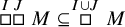 , and
$\stackrel {I}{\Box }M$
 is closed provided that M is closed. Moreover,
$\stackrel {I}{\Box } (M_1 \cup M_2) =\stackrel {I}{\Box }M_1 \cup \stackrel {I}{\Box }M_2$
 .
The following lemma is a crucial step for proving that
$\Gamma ^{\infty }(A) = Y_A^2$
 for countable A.
Proposition 5.8. Let
$A \in \mathcal {K}$
 ,
$I \subseteq (0,1)$
 be an interval and G be a countable collection of pairwise disjoint subintervals of I such that
$I \cap L(A) \subseteq \cup G$
 . Furthermore, let
$f \in Y$
 ,
$t: I[ \cap L(A) \rightarrow Y$
 and
$\{H_J\}_{J\in G}$
 be a family of closed subsets of
$Y_A^2$
 , such that for every
$J\in G$
 we have the following properties.
-
1. For all $(y,y') \in H_J$
, we have
$y \stackrel {J} {\asymp } y'$
. -
2. For all $(y,y') \in H_J$
,
$y|_{I \cap J[} =f$
, and
$y|_{I[} =t$
. -
3. For all $w \in Y_A$
, there is
$(y,y') \in H_J$
such that
$w|_{]J} = y|_{]J} $
. -
4. $\stackrel {J}{\Box }{H_J}= H_J$
.


Then, letting
$H= \bigcup _{J \in G}H_J$
 , we have
$\stackrel {I}{\Box }H \subseteq \Gamma (\overline {H})$
 .
Proof. If
$I \cap L(A) = \emptyset $
 , then
$\stackrel {I}{\Box }H = H$
 and as
$H \subseteq \Gamma (\overline {H})$
 , we are done. Hence, assume that
$I \cap L(A) \neq \emptyset $
 . Note that all
$(y,y') \in H$
 have the property that
$y \stackrel {I} {\asymp } y'$
 and
$y|_{I[} =t$
 . Considering this and Property 3, we obtain that

As such, to conclude that
$\stackrel {I}{\Box }H \subseteq \Gamma (\overline {H})$
 , it will suffice to show that for all
$v_0 \in Y_A$
 ,
$F \subseteq I \cap L(A)$
 nonempty finite set, and
$u, u': F \rightarrow Y$
 , there exists
$(w,w') \in H^+$
 such that
$w|_{]I} =v_0|_{]I}$
 and
$w,w'$
 are extensions of
$u,u'$
 , respectively. Moreover, as equivalence relations are symmetric and transitive, we may assume that
$u'$
 is a constant function taking value f. Let
$J_1, \ldots , J_n$
 be intervals in G so that
$F \subseteq \cup _{i=1}^n J_i$
 and
$J_i$
 is to the left of
$J_{i+1}$
 . Fix i for the moment. By applying Properties 1–4 to
$J_i$
 , we have that for all
$v \in Y_A$
 , there exists
$(y,y') \in H_{J_i}$
 so that
-
• $y|_{]J_i} = y'|_{]J_i}= v|_{]J_i}$
, -
• $y'|_{J_i}=f$
, y and u agree on
$F \cap J_i$
, -
• $y|_{I \cap J_i[} = y'|_{I \cap J_i[} =f$
and
$y|_{I[} = y'|_{I[} =t$
.


Applying the above observation with
$i=1$
 and
$v=v_0$
 , we obtain
$(w_0,w_1) \in H_{J_1}$
 so that
$w_0|_{]J_1}=w_1|_{]J_1} =v_0$
 ,
$w_0|_{J_1}=f$
 ,
$w_1$
 is u on
$F\cap J_1$
 ,
$w_0|_{I \cap J_1[} = w_1|_{I \cap J_1[} =f$
 and
$w_0|_{I[} = w_1|_{I[} =t$
 . Now, we apply the observation with
$i=2$
 , and
$v=w_1$
 . Hence, we obtain
$(y,w_2) \in H_{J_2}$
 so that
$y|_{]J_2}=w_2|_{]J_2} =w_1$
 ,
$y|_{J_2}=f$
 ,
$w_2$
 is u on
$F\cap J_2$
 ,
$y_0|_{I \cap J_2[} = w_2|_{I \cap J_2[} =f$
 and
$y|_{I[} = w_2|_{I[} =t$
 . Note that necessarily
$y=w_1$
 . Hence, it holds
$(w_0,w_1), (w_1, w_2) \in H$
 , that is,
$(w_0,w_2) \in H^+$
 . Continuing in this fashion, setting
$v=w_{i-1}$
 at stage i, we arrive at
$(w_0,w_n) \in H^+$
 so that
$w_n =u$
 on F,
$w_0$
 is the constant f on F and
$w_0|_{]I}=w_1|_{]I}=v_0$
 , completing the proof of
$\stackrel {I}{\Box }H \subseteq \Gamma (\overline {H})$
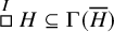 .
Let
$I \subseteq (0,1)$
 . For the rest of this section we let

We note that
$E_I$
 depends on A but A is suppressed in the notation for the sake of brevity.
Proposition 5.9. Let
$A \in \mathcal {K}$
 ,
$I \subseteq (0,1)$
 , and
$M \subseteq Y_A ^2$
 be such that for all
$(y,y') \in M$
 ,
$y = y'$
 on
$ L(A) \setminus I$
 . Then,
$ (\stackrel {I}{\Box } M )^+ = \stackrel {I}{\Box } M$
 . In particular,
$E_I^+ = E_I$
 for all
$I \subseteq (0,1)$
 .
Proof. To show that
$ (\stackrel {I}{\Box } M )^+ \subseteq \stackrel {I}{\Box } M$
 , let
$(u,v),(v,w)\in \stackrel {I}{\Box }M$
 . This implies there exist
$(x,x'),(y,y')\in M$
 such that
$u \stackrel {I} {\asymp } x$
 ,
$v \stackrel {I} {\asymp } x'$
 ,
$v \stackrel {I} {\asymp } y'$
 and
$w \stackrel {I} {\asymp } y'$
 . Using the hypothesis we conclude that
$x' \stackrel {I} {\asymp } w$
 , hence
$(u,w)\in \stackrel {I}{\Box }M$
 .
Proposition 5.10. Let
$A \in \mathcal {K}$
 ,
$\alpha $
 be a countable ordinal and
$I = (0,1)$
 or
$I\in \mathcal {C}(A^{\alpha +1})$
 . Let G be the set of all
$J \in \mathcal {C}(A^{\alpha })$
 such that
$J \subseteq I$
 . Then,
$ \bigcup _{J \in G} E_{\overset {\bullet\!- }{J}} \bigcup \Delta _{Y_A} $
 is closed.
Proof. We first show that
$E_{\overset {\bullet\!- }{J}}$
 is closed for all
$J \in \mathcal {C}(A^{\alpha })$
 . By Proposition 5.2, there is
$t:L(A) \cap J[ \rightarrow A$
 such that for all
$(y,y') \in D_a$
 ,
$a \in L(A) \cap \overset {\bullet\!- }{J}$
 , we have
$y|_{J[} = y'|_{J[} = t$
 . Now, from the definitions of
$D_a$
 and
$\stackrel {\overset {\bullet\!- }{J}}{\Box }$
 , the following holds

implying that
$E_{\overset {\bullet\!- }{J}}$
 is closed.
Let
$E = \bigcup _{J \in G} E_{\overset {\bullet\!- }{J}}\bigcup \Delta _{Y_A} $
 . To show that E is closed, let
$\{(y_n, y^{\prime }_n)\}$
 be a sequence in
$\bigcup _{J \in G} E_{\overset {\bullet\!- }{J}}$
 that converges to
$(y,y')\in Y_A^2$
 . Let
$J_n \in G$
 such that
$ (y_n,y^{\prime }_n) \in E_{\overset {\bullet\!- }{J_n}}$
 . If there is
$J \in G$
 such that
$J_n = J$
 for infinitely many n’s, then by the fact that
$E_{\overset {\bullet\!- }{J}}$
 is closed we have
$(y,y') \in E_{\overset {\bullet\!- }{J}} \subseteq E$
 and we are done. Hence, we may assume that
$J_n$
 ’s are all distinct. Since
$ (y_n,y^{\prime }_n) \in E_{\overset {\bullet\!- }{J_n}}$
 , this implies that for every
$p\in L(A)$
 ,
$y_n(p)=y^{\prime }_n(p)$
 for all but at most one n. Hence,
$y=y'$
 . As
$\Delta _{Y_A} \subseteq E$
 , the proof is complete.
Let
$A \in \mathcal {K}$
 and
$\alpha $
 be a countable ordinal. Then, we define

Proposition 5.11. Let
$A \in \mathcal {K}$
 . we have
$D_A \subseteq E_{\alpha }$
 ,
$E_{\alpha }$
 is closed, and if
$\alpha $
 is a limit ordinal, then
$E_{\alpha } = \overline { \cup _{\beta < \alpha } E_{\beta }}$
 .
Proof. That
$D_A \subseteq E_{\alpha }$
 follows from the fact that if
$J \in \mathcal {C}(A)$
 , then
$J \subseteq I$
 for some
$I \in \mathcal {C}(A^{\alpha })$
 . Note that
$\Delta _{Y_A} \subseteq D_{\max A} \subseteq E_{\alpha }$
 . Now that
$E_{\alpha }$
 is closed follows from Proposition 5.10.
Suppose
$\alpha $
 is a limit ordinal. For each
$\beta < \alpha $
 ,
$E_{\beta } \subseteq E_{\alpha }$
 . As
$E_{\alpha }$
 is closed, we have the containment
$E_{\alpha } \supseteq \overline { \cup _{\beta < \alpha } E_{\beta }}$
 . To see the reverse containment, let
$(y,y') \in E_{\alpha }$
 . By the definition of
$E_{\alpha }$
 , there is
$ I\in \mathcal {C}(A^{\alpha })$
 ,
$a \in \overset {\bullet\!- }{I}$
 and
$(w,w') \in D_a$
 such that
$w \stackrel {\overset {\bullet\!- }{I}} {\asymp } y, w' \stackrel {\overset {\bullet\!- }{I}} {\asymp } y'$
 . Let
$a_1 < \ldots < a_n$
 be in
$L(A)$
 and
$(U_1,V_1), \ldots ,(U_n,V_n)$
 be open sets in
$Y^2$
 such that
$(y(a_i),y'(a_i)) \in (U_i,V_i)$
 . To complete the proof, it suffices to show that there is
$\beta < \alpha $
 and
$(z,z') \in E_{\beta }$
 such that
$(z(a_i),z'(a_i)) \in (U_i,V_i)$
 . By enlarging, if necessary, we assume that a is one of the
$a_i$
 ’s. As
$\alpha $
 is a limit ordinal, then
$A^{\beta } \rightarrow A^{\alpha }$
 in the Hausdorff metric as
$\beta \rightarrow \alpha $
 . Hence, we may choose
$\beta <\alpha $
 sufficiently large so that there is
$J \in \mathcal {C}(A^{\beta })$
 such
$I \cap \{a_1, \ldots , a_n\} \subseteq {J} \subseteq {I}$
 . Moreover, if
$\ell (I) \in L(A)$
 , we may obtain J so that, in addition, that
$\ell (J) = \ell (I)$
 . Hence, for sufficiently large
$\beta $
 we have that
${\overset {\bullet\!- }{I}} \cap \{a_1, \ldots , a_n\} \subseteq {\overset {\bullet\!- }{J}} \subseteq {\overset {\bullet\!- }{I}}$
 . We define
$z, z'$
 in the following fashion:
$z = w$
 ,
$z' = w'$
 on
$L(A) \setminus \overset {\bullet\!- }{J}$
 ,
$z(a_i)= y(a_i)$
 ,
$z'(a_i) = y'(a_i)$
 for all
$a_i$
 ’s in
$\overset {\bullet\!- }{J}$
 and
$z(b) = w(b)$
 ,
$z'(b) = w'(b)$
 for
$b \in (L(A) \cap \overset {\bullet\!- }{J} ) \setminus \{a_1, \ldots , a_n\}$
 . Note that
$w \stackrel {\overset {\bullet\!- }{J}} {\asymp } z, w' \stackrel {\overset {\bullet\!- }{J}} {\asymp } z'$
 and as
$a \in \overset {\bullet\!- }{I} \cap \{a_1, \ldots , a_n\} \subseteq \overset {\bullet\!- }{J} $
 and
$(w,w') \in D_a$
 , then
$(z,z') \in E_{\overset {\bullet\!- }{J}} \subseteq E_{\beta }$
 . If
$a_i \in \overset {\bullet\!- }{I}$
 , then
$a_i \in \overset {\bullet\!- }{J}$
 and hence
$z(a_i) = y(a_i)$
 and
$z'(a_i)=y'(a_i)$
 , implying that
$(z(a_i),z'(a_i)) \in (U_i, V_i)$
 . If
$a_i \notin \overset {\bullet\!- }{I}$
 , then
$a_i \notin \overset {\bullet\!- }{J} $
 . In this case, we have
$z(a_i) = w(a_i) = y(a_i)$
 as
$w \stackrel {\overset {\bullet\!- }{I}} {\asymp } y$
 and similarly
$z'(a_i) = y'(a_i)$
 , yielding that
$(z(a_i), z'(a_i)) \in (U_i, V_i)$
 and completing the proof.
Proposition 5.12. Let
$A \in \mathcal {K}$
 and
$\alpha $
 be a countable ordinal. If
$I, J \in \mathcal {C} (A^{\alpha })$
 are disjoint with
$L(A) \cap \overset {\bullet\!- }{I} \neq \emptyset $
 and
$L(A) \cap \overset {\bullet\!- }{J} \neq \emptyset $
 , then
$E_{\alpha } \neq Y_A^2$
 .
Proof. Let
$a \in L(A) \cap \overset {\bullet\!- }{I}$
 and
$b \in L(A) \cap \overset {\bullet\!- }{J}$
 . Let
$(y,y') \in E_{\alpha }$
 . By the definitions of
$D_A$
 , the properties of I of J and definition of
$E_{\alpha }$
 , then either
$y(a) = y'(a)$
 or
$y(b)= y'(b)$
 , implying that
$E_{\alpha } \neq Y_A^2$
 .
Proposition 5.13. Let
$A \in \mathcal {K}$
 and
$\alpha $
 be a countable ordinal such that
$A^{\alpha } \neq \emptyset $
 . Let
$I \in \mathcal {C}(A^{\alpha +1})$
 and let G be the collection of
$\overset {\bullet\!- }{J}$
 such that
$J \in \mathcal {C}(A^{\alpha })$
 ,
$J \subseteq I$
 , and
$\overset {\bullet\!- }{J} \cap L(A) \neq \emptyset $
 . Then, G is a collection of pairwise disjoint intervals such that
$\overset {\bullet\!- }{I} \cap L(A) \subseteq \cup G$
 .
Proof. That G is pairwise disjoint is clear as elements of
$\mathcal {C}(A^{\alpha })$
 are pairwise disjoint open intervals. Let
$a \in \overset {\bullet\!- }{I} \cap L(A)$
 . If
$a \in I \setminus A^{\alpha }$
 , then a is in some interval contiguous to
$A^{\alpha }$
 which is a subset of I and we are done. Now suppose that
$a \in A^{\alpha }$
 . Recall that by the fact that
$a \in L(A)$
 , a is the left endpoint of some open interval contiguous to A. That interval is a subset of some open interval J contiguous to
$A^{\alpha }$
 . As
$a \in A^{\alpha }$
 , the left endpoint of J is a. As
$a \in \overset {\bullet\!- }{I}$
 , then
$J \subseteq I$
 . Then
$a \in \overset {\bullet\!- }{J} \in G$
 , concluding the proof.
Proposition 5.14. Let
$A \in \mathcal {K}$
 and
$\alpha $
 be a countable ordinal such that
$A^{\alpha } \neq \emptyset $
 . Then,
$E_{\alpha +1} \subseteq \Gamma (E_{\alpha })$
 .
Proof. Let
$I \in \mathcal {C}(A^{\alpha +1})$
 . It will suffice to show that
$E_{\overset {\bullet\!- }{I}} \subseteq \Gamma (E_{\alpha })$
 . Let

We will apply Proposition 5.8 to
$\overset {\bullet\!- }{I}$
 , G, and
$H_J = E_J$
 to conclude
$E_{\overset {\bullet\!- }{I}} \subseteq \Gamma (E_{\alpha })$
 . We commence by verifying the hypotheses of Proposition 5.8. By Proposition 5.13, G is a collection of pairwise disjoint subintervals of
$\overset {\bullet\!- }{I}$
 with
$\overset {\bullet\!- }{I} \cap L(A) \subseteq \cup G$
 . Next choose f according to Proposition 5.4 and let
$t=t_I$
 . Let us check that Properties 1–4 of Proposition 5.8 are satisfied. Property 1 follows simply from the definition of
$D_a$
 and
$E_J$
 . To see Property 2, let
$(y,y') \in E_J$
 . By the definition of
$\Box $
 ,
$(y,y')$
 is obtained from some
$D_a$
 ,
$a \in J \cap L(A)$
 . By Proposition 5.4, we have
$y|_{\overset {\bullet\!- }{I} \cap J[}= t_a|_{\overset {\bullet\!- }{I} \cap J[}=f$
 . Analogously, Proposition 5.2 implies that
$y|_{\overset {\bullet\!- }{I}[} =t$
 . To see Property 3, note that as
$\overset {\bullet\!- }{J} \cap L(A) \neq \emptyset $
 , some
$D_a$
 is a subset of
$E_J$
 . Property 4 is clear by the definition of
$E_J$
 . Finally, set
$H= \bigcup _{J \in G} E_J$
 . By Proposition 5.10 and the fact that
$\Delta _{Y_A} \subseteq E_{\alpha }$
 , the following holds

Now drawing on the conclusion of Proposition 5.8, we have

As
$\overset {\bullet\!- }{I} \cap L(A) \subseteq \bigcup G$
 , then
$\bigcup _{a \in \overset {\bullet\!- }{I} \cap L(A) } D_a \subseteq H $
 , implying that
$\stackrel {\overset {\bullet\!- }{I}}{\Box }H \supseteq E_{\overset {\bullet\!- }{I}}$
 and concluding the proof of
$E_{\alpha +1} \subseteq \Gamma (E_{\alpha })$
 .
Proposition 5.15. Let
$A \in \mathcal {K}$
 and
$\alpha $
 be a countable ordinal such that
$A^{\alpha } \neq \emptyset $
 . Then,

Proof. We proceed by induction on
$\alpha $
 . At stage
$\alpha =0$
 , the following holds

Suppose that
$\alpha>0$
 is a countable ordinal such that for all
$\beta < \alpha $
 we have
$E_{\beta } \subseteq \Gamma ^{\beta } (D_A)$
 . If
$\alpha $
 is a limit ordinal, then

where the rightmost equality follows by Proposition 5.11. If
$\alpha $
 is a successor ordinal, then Proposition 5.14 and the induction hypothesis give

Next we would like to study the situation when
$A^{\infty } \neq \emptyset $
 . It may seem that in this situation,
$\Gamma (E_{\alpha }) = E_{\alpha }$
 where
$\alpha = |A|_{CB}$
 . Unfortunately, such is not the case. We modify
$E_{\alpha }$
 appropriately to obtain a set E for which
$\Gamma (E) = E$
 .
Proposition 5.16. Let
$A \in \mathcal {K}$
 with
$A^{\infty } \neq \emptyset $
 ,
$\alpha = |A|_{CB}$
 , and
$I_e\in \mathcal {C}(A^{\alpha })$
 be such that
$r(I_e) =1$
 . We set

Then,
$D_A \subseteq E$
 , E is closed and
$\Gamma (E) = E$
 . Moreover,
$E \neq Y_A^2$
 .
Proof. That
$D_A \subseteq E$
 follows from the fact that
$D_A=E_0 \subseteq E_{\alpha } \subseteq E$
 . Using that
$\Box $
 is distributive over unions, Remark 5.7, then

As
$E_{\alpha }$
 is closed and
$\Box $
 of a closed set is closed, then
$E $
 is closed.
To prove that
$\Gamma (E) = E$
 , first we will show that
$E^+ = E$
 . By Proposition 5.9,
$ \left (\stackrel {I_e}{\Box } E_{\overset {\bullet\!- }{I}} \right ) ^+ = \stackrel {I_e}{\Box } E_{\overset {\bullet\!- }{I}}$
 for all
$I \in \mathcal {C} (A^{\infty })$
 . As such, it will suffice to show that if
$I, J \in \mathcal {C} (A^{\infty })$
 are distinct,
$(y,y') \in \stackrel {I_e}{\Box } E_{\overset {\bullet\!- }{I}}$
 , and
$(y',y") \in \stackrel {I_e}{\Box } E_{\overset {\bullet\!- }{J}}$
 , then
$(y,y") \in E$
 . Without loss of generality, assume that I is to the left of J. Using the definition of
$E_{\overset {\bullet\!- }{I}}$
 , and Remark 5.7, there exists
$a \in \overset {\bullet\!- }{I}$
 and
$(w_1,w_2) \in D_a$
 such that
$ w_1 \stackrel {\overset {\bullet\!- }{I} \cup \overset {\bullet\!- }{I_e}} {\asymp } y$
 and
$ w_2 \stackrel {\overset {\bullet\!- }{I} \cup \overset {\bullet\!- }{I_e}} {\asymp } y'$
 . Similarly, let
$b \in \overset {\bullet\!- }{J}$
 and
$(w_3,w_4) \in D_b$
 such that
$ w_3 \stackrel {\overset {\bullet\!- }{I} \cup \overset {\bullet\!- }{I_e}} {\asymp } y '$
 and
$ w_4 \stackrel {\overset {\bullet\!- }{I} \cup \overset {\bullet\!- }{I_e}} {\asymp } y"$
 . We now show that J must equal to
$I_e$
 . Suppose such is not the case. As
$A^{\infty }$
 is perfect we have that between any two elements of
$\mathcal {C}(A^{\infty })$
 there is an element of
$\mathcal {C}(A^{\infty })$
 . Moreover, every element of
$\mathcal {C}(A^{\infty })$
 whose endpoint is not
$0$
 contains a point of
$L(A)$
 . Hence, we may choose some
$c \in L(A) \cap J[ $
 such that
$ c \notin \overset {\bullet\!- }{I_e}$
 . Using Proposition 5.3, the definition of
$D_A$
 and the fact that
$(w_1,w_2) \in D_a$
 , we conclude that
$ w_1(c) = w_2(c) =r (I)$
 . As
$ w_1 \stackrel {\overset {\bullet\!- }{I} \cup \overset {\bullet\!- }{I_e}} {\asymp } y$
 ,
$ w_2 \stackrel {\overset {\bullet\!- }{I} \cup \overset {\bullet\!- }{I_e}} {\asymp } y'$
 ,
$c \in L(A) \in J[ $
 and
$ c \notin ]\overset {\bullet\!- }{I_e}$
 , we have
$ y(c) = y'(c) =r (I)$
 . Arguing similarly with
$(w_3,w_4)$
 , we conclude that
$ y'(c) = y"(c) =r (J)$
 , yielding a contradiction as I and J are disjoint intervals. Hence we have shown that
$J =I_e$
 . We now show that
$(y,y") \in \stackrel {I_e}{\Box } E_{\overset {\bullet\!- }{I}}$
 to complete the proof of
$\Gamma (E) = E$
 . It will suffice to show that
$w_2 \stackrel {\overset {\bullet\!- }{I} \cup \overset {\bullet\!- }{I_e}} {\asymp } y"$
 as already
$ w_1 \stackrel {\overset {\bullet\!- }{I} \cup \overset {\bullet\!- }{I_e}} {\asymp } y$
 . Indeed,
$y" = y'$
 on
$L(A) \setminus \overset {\bullet\!- }{I_e}$
 , and
$y' = w_2$
 on
$L(A) \setminus (\overset {\bullet\!- }{I} \cup \overset {\bullet\!- }{I_e})$
 , implying that
$y" = w_2$
 on
$L(A) \setminus (\overset {\bullet\!- }{I} \cup \overset {\bullet\!- }{I_e})$
 , that is,
$w_2 \stackrel {\overset {\bullet\!- }{I} \cup \overset {\bullet\!- }{I_e}} {\asymp } y"$
 .
Finally, we show that
$E \neq Y_A^2$
 to complete the proof of the proposition. Choose
$I, J \in \mathcal {C}(A^{\infty })$
 with neither one being
$I_e$
 and
$a \in L(A) \cap \overset {\bullet\!- }{I} $
 and
$b \in L(A) \cap \overset {\bullet\!- }{J}$
 . Let
$(y,y') \in E$
 . By the definitions of
$D_A$
 and E, then either
$y(a) = y'(a)$
 or
$y(b)= y'(b)$
 , implying that
$E \neq Y_A^2$
 .
Corollary 5.17. A set
$A \in \mathcal {K}$
 is countable if and only if
$\Gamma ^{\infty }(D_A) = Y_A ^2$
 .
Proof. Let
$\beta = | A |_{CB}$
 .
If A is countable, then
$\beta $
 is necessarily a successor ordinal and
$A^{\beta } = \emptyset $
 . This implies that

Applying Proposition 5.15 to
$\alpha = \beta -1$
 , we obtain
$E_{\beta } \subseteq \Gamma ^{\alpha }(D_A)$
 . Hence,
$\Gamma ^{\infty }(D_A) = Y_A ^2$
 .
If A is uncountable, then
$\Gamma ^{\infty }(D_A) \neq Y_A ^2$
 follows simply from Proposition 5.16.
Proposition 5.18. For each countable ordinal
$\alpha $
 , there exists
$A \in \mathcal {K}$
 so that the
$\Gamma $
 -rank of
$B_A$
 is greater than
$\alpha $
 .
Proof. Let
$\alpha $
 be a countable ordinal. Let
$A \in \mathcal {K}$
 be a countable compact set such that
$|A|_{CB}> \alpha +1$
 and
$A^{|A|_{CB}-1} = \{\max (A)\}$
 . For the sake of brevity, let
$e = \max (A)$
 and
$I_e \in \mathcal {C}(A)$
 with
$\ell (I_e) = e$
 . By our choices of A we get
$I_e \in \mathcal {C}(A^{\beta })$
 for all
$\beta < |A|_{CB}$
 .
Let us first prove that
$\Gamma (D_A) = \Gamma (E_0)= \stackrel {e}{\Box } E_{1}.$
 For each
$J \in \mathcal {C}(A)$
 , the following holds

Next, if
$J_1, J_2 \in \mathcal {C}(A)$
 with
$J_i \subseteq I_i \in \mathcal {C}(A')$
 with neither
$I_i$
 equal to
$I_e$
 , and
$I_1 \neq I_2$
 , then

This is so because there is
$I_3 \in \mathcal {C}(A')$
 which is to the right of
$I_1,I_2$
 and to the left of
$I_e$
 . For
$a \in L(A) \cap I_3$
 , we obtain
$t_{I_1}(a) \neq t_{I_2}(a)$
 . Hence (2) follows. Next, fix
$I \in \mathcal {C}(A')$
 momentarily. Arguing as in the proof of Proposition 5.8 with
$H_J = \stackrel {e}{\Box }E_{\overset {\bullet\!- }{J}}$
 ,
$J \in \mathcal {C}(A)$
 ,
$J \subseteq I$
 , and using (2) from above, we obtain

Finally, putting (1), (2) and (3) together, we get

The last equality follows from the fact that
$E_1$
 is closed.
The general
$\alpha $
 case is analogous to the above. Arguing in the same fashion, we have
$\Gamma ^{\beta } (D_A)=\Gamma ^{\beta } (E_0) = \stackrel {e}{\Box } E_{\beta + 1}$
 , for all
$\beta < |A|_{CB}$
 . As
$A^{|A|_{CB}-2}$
 is an infinite set, then
$\stackrel {e}{\Box } E_{|A|_{CB}-2} \neq Y_A^2$
 , implying that the
$\Gamma $
 -rank of
$D_A$
 , and hence of
$B_A$
 , is greater than or equal to
$|A|_{CB}-1> \alpha $
 .
5.2 Entropy construction
The main objective of this subsection is to translate Proposition 5.18 to the language of entropy pairs, and check that the phase space is indeed a Cantor space.
In this subsection, we will map
$(Y_A,R_A,B_A)$
 from the previous section to a dynamical system
$(X_A,T_A)$
 so that
$\Gamma ^{\infty }(B_A)=Y_A^2$
 if and only if
$\Gamma ^{\infty }(E(X_A,T_A))=X_A^2$
 .
Fix
$A \in \mathcal {K}$
 and let
$(Y_A,R_A,B_A)$
 be as defined in the last section. We continue to use the notation of the previous section. Recall that for
$a\in L(A)$
 ,
$I \in \mathcal {C}(A)$
 with
$a= \ell (I)$
 ,


We will construct
$X_A$
 as a factor. We let
$Z_{A}=X\times Y_{A}$
 be our intermediate space. Points in
$Z_{A}$
 are represented as
$xy$
 , with
$x\in X$
 and
$y\in Y_A$
 . For
$a\in L(A)$
 ,
$I \in \mathcal {C}(A)$
 with
$a= \ell (I)$
 , we let


Lemma 5.19. If
$(y,y') \in B_A$
 , then there is
$x \in X $
 such that
$(xy,xy') \in F_A$
 .
Proof. Let
$(y,y') \in B_A$
 . If
$y=y'$
 , then for any
$x \in X$
 we get
$(xy,xy') \in F_A$
 as
$\Delta _{Z_{A}} \subseteq F_A$
 . If
$y \neq y'$
 , then
$(y,y') \in B_a$
 for some
$a \in L(A)$
 and
$\{y(a),y'(a)\} \in R$
 . Without loss of generality, assume that
$R(y(a)) = y'(a)$
 . Then, letting
$x = y(a)$
 we conclude that
$(xy,xy') \in F_a \subseteq F_A$
 .
Lemma 5.20. We have
$F_{A}$
 is an equivalence relation which is a closed subset of
$Z_A^2$
 . Moreover,
$F_A$
 is
$T\times R_{A}$
 -invariant.
Proof. That
$F_A$
 is a closed subset of
$Z_A^2$
 follows from the fact that
$B_A$
 is a closed subset of
$Y_A ^2$
 (Proposition 5.5).
$B_A$
 is
$R_A$
 -invariant as the range of
$t_a$
 ,
$a \in L(A)$
 , is a subset of
$C \subseteq \text {fix}(Y,R)$
 . This implies that
$F_A$
 is
$T\times R_{A}$
 -invariant. That
$\Delta _{Z_{A}}\subseteq F_{A}$
 follows from the definition of
$F_A$
 . As
$B_A$
 is symmetric, so is
$F_{A}$
 .
Finally, we show that
$F_A$
 is transitive, that is,
$F_A^+ = F_A$
 . Let
$(xy,xy^{\prime }),(xy^{\prime },x y^{\prime \prime })\in F_{A}$
 . If
$y = y'$
 or
$y' =y"$
 , then obviously
$(xy,xy^{\prime \prime })\in F_{A}$
 . Hence, assume that
$y\neq y^{\prime }\neq y^{\prime \prime }$
 . Let
$a, a^{\prime }\in L(A)$
 be the only points where
$y(a)\neq y^{\prime }(a)$
 and
$y^{\prime } (a^{\prime })\neq y^{\prime \prime }(a^{\prime })$
 . By hypothesis, we have
$\{y(a),y^{\prime }(a)\}=\{y^{\prime }(a^{\prime }),y^{\prime \prime }(a^{\prime })\}=\{ x,Tx\}$
 . Since
$y\neq y'$
 then
$Tx\neq x$
 . We next show that
$a = a'$
 . To obtain a contradiction, assume that
$a<a'$
 . Since
$(y,y')\in B_a$
 then
$y'(a') = t_a(a')$
 which by construction is a fixed point of R, yielding a contradiction. Hence,
$a=a^{\prime }$
 . Using
$a=a^{\prime }$
 and that
$\{y(a),y^{\prime }(a)\}=\{y^{\prime }(a^{\prime }),y^{\prime \prime }(a^{\prime })\}=\{ x,Tx\}$
 , we obtain
$y(a)=y"(a)$
 , implying that
$y =y"$
 . As
$\Delta _{Z_{A}}\subseteq F_{A}$
 , we get
$(xy,xy") =(xy,xy) \in F_A$
 , completing the proof.
Let
$X_{A}=Z_{A}/F_{A}$
 endowed with the quotient topology. As
$Z_{A}$
 is a compact metrizable space and
$F_{A}$
 a closed set and an equivalence relation, we have that
$X_{A}$
 is a compact metrizable space (?, Theorem 4.2.13). Let
$P_{A}:Z_{A}\rightarrow X_{A}$
 be projection induced by
$F_{A}$
 and define
$T_{A}:X_{A}\rightarrow X_{A}$
 by
$T_{A} ([z]_{F_{A}})=[(T\times R_{A})(z)]_{F_{A}}$
 , where
$[z]_{F_{A}}$
 denotes the equivalence class of
$z\in Z_{A}$
 in
$F_{A}$
 . As
$F_{A}$
 is invariant under
$T\times R_{A}$
 , then
$T_{A}$
 is well-defined and continuous. Moreover,
$P_{A}\circ (T\times R_{A})=T_{A}\circ P_{A}$
 . In particular,
$(X_{A},T_{A})$
 is a factor of
$(Z_{A},T\times R_{A})$
 , that is, the following diagram commutes.

As the product of mixing maps is mixing, then
$T\times R_{A}$
 is mixing. As
$P_{A}$
 is surjective, and mixing is preserved under factor maps, we have that
$(X_{A},T_{A})$
 is mixing as well.
Lemma 5.21. Let
$A\in \mathcal {K}$
 . We have

Proof. Recall from Lemma 5.1 that
$E(Y_{A},R_{A})=\Delta _{Y_{A}}$
 and
$E(X,T)=X^{2}$
 . Using these facts and Theorem 2.4 (2) we obtain that

Using Theorem 2.4 (3) we get

It follows that

To prove the second
$\subseteq $
 , let
$x, x' \in X$
 and
$(y,y')\in B_A$
 . Then, by Lemma 5.19, there exists
$x"\in X$
 such that

Moreover, we have

implying that
$([xy]_{F_A},[x'y']_{F_A}) \in E(X_A,T_A)^+$
 and concluding the proof.
Theorem 5.22. Let
$A\in \mathcal {K}$
 . Then, the entropy rank of
$(X_A,T_A)$
 is greater than or equal to the
$\Gamma $
 -rank of
$B_A$
 , and

In particular, we get
$\Gamma ^{\infty }(B_A)=Y_A^2$
 if and only if
$\Gamma ^{\infty }(E(X_A,T_A))=X_A^2$
 .
Proof. Let

By Lemma 5.21, we get

for every countable ordinal
$\alpha $
 . We next prove by induction that

Assume the result holds for every
$\beta ^{\prime }<\beta $
 . If
$\beta $
 is a successor, then it is easy to check

If
$\beta $
 is a limit ordinal, one can show that

Now using the continuity of
$P_A$
 , we conclude that (*) holds.
Returning to the main proof, by (*), the
$\Gamma $
 -rank of G is the same as the
$\Gamma $
 -rank of
$B_A$
 . As
$E(X_A,T_A) \subseteq G$
 , we get that the
$\Gamma $
 -rank of G is less than or equal to the entropy rank of
$(X_A,T_A)$
 , or equivalently, the entropy rank of
$(X_A,T_A)$
 is greater than or equal to
$\Gamma $
 -rank of
$B_A$
 . Finally, the second claim of the theorem follows from the fact that,

for every countable ordinal
$\alpha $
 .
Corollary 5.23. Let
$\alpha $
 be a countable ordinal. Then there is a countable set
$A \in \mathcal {K}$
 such that
$(X_A,T_A)$
 has completely positive entropy and its entropy rank is greater than
$\alpha $
 .
Proof. Let
$A \in \mathcal {K}$
 be a countable set in the statement of Proposition 5.18. By Corollary 5.17 and Remark 5.6, we have
$\Gamma ^{\infty }(B_A)=Y_A^2$
 . Now by Theorem 5.22, we conclude that the entropy rank of
$(X_A,T_A)$
 is greater than
$\alpha $
 and
$\Gamma ^{\infty }(E(X_A,T_A))=X_A^2$
 , that is,
$(X_A,T_A)$
 has CPE.
Theorem 5.24. For each
$A\in \mathcal {K}$
 ,
$X_{A}$
 is a Cantor space.
Proof. We will show that
$X_A$
 has no isolated points and
$X_A$
 is totally disconnected. To see that
$X_A$
 is totally disconnected, let
$([xy]_{F_{A}},[x'y^{\prime }]_{F_{A}})\in X_{A}^{2}\backslash \Delta _{X_{A}}$
 . We will show that there exists a clopen set of
$X_A$
 which contains one but not the other.
Recall that
$P_{A}:Z_{A}\rightarrow X_{A}$
 is a surjection and
$X_A$
 is equipped with quotient topology. Hence, if
$D \subseteq X_A$
 and
$P_{A}^{-1}(D)$
 is clopen in
$Z_A$
 , then D is clopen in
$X_A$
 .
Case 1: Suppose that
$x\neq x'$
 . As X is zero-dimensional, we may choose a clopen set
$B\subseteq X$
 such that
$x\in B$
 and
$x'\notin B$
 . Then,
$D=B\times Y_{A}$
 is a clopen set. One can check that
$P_{A}^{-1}([D]_{F_{A}})=D$
 . Hence,
$[D]_{F_{A}}$
 is a clopen set such that
$[xy]_{F_{A}}\in [D]_{F_{A}}$
 and
$[x^{\prime }y^{\prime }]_{F_{A}}\notin [ D]_{F_{A}}$
 .
Case 2: Suppose that
$x = x'$
 . Since
$[xy]_{F_{A}}\neq \lbrack xy^{\prime }]_{F_{A}}$
 , without loss of generality, we may assume that there exists
$b\in L(A)$
 such that
$y(b)\neq y'(b)$
 and
$y(b)\notin \left \{x,T(x)\right \}.$
 Let
$B\subseteq X$
 be a clopen set such that
$y(b)\notin B$
 ,
$\{ x,T(x),y'(b)\}\subseteq B$
 , and using the continuity of T let
$F\subseteq B$
 be a clopen set such that
$x\in F$
 ,
$F\cup T(F)\subseteq B$
 .
We define

and

Observe that for
$k\in K$
 and
$k' \in [k]_{F_A}$
 , the equality
$k(b) = k'(b)$
 holds. From this it follows that
$[k]_{F_A}\subseteq K$
 . Hence,
$P_{A}^{-1}([ K]_{F_{A}\text { }})= K$
 , implying that
$[ K]_{F_{A}}$
 is clopen. Furthermore,
$[xy]_{F_{A}} \in \lbrack K]_{F_{A}}$
 and
$[xy^{\prime }]_{F_{A}}\notin \lbrack K]_{F_{A}}$
 .
With these two cases we conclude that
$X_A$
 is totally disconnected.
To see that
$X_A$
 has no isolated points, note that X and hence
$Z_A$
 has no isolated points. Moreover,
$P_A$
 is an at most two-to-one map, implying that
$X_A$
 has no isolated point.
Theorem 5.25. Let X be a Cantor space. Then,
$\text {Mix}(X) \cap \text {CPE}(X)$
 is a coanalytic subset that is not Borel.
Proof. That
$\text {Mix}(X) \cap \text {CPE}(X)$
 is coanalytic follows from the facts that
$\text {Mix}(X)$
 is Borel (Remark 3.8), and
$\text {CPE}(X)$
 is coanalytic (Proposition 2.13). By Proposition 2.14, we have that entropy rank is a
$\Pi ^1_1$
 -rank. By Corollary 5.23 and Theorem 5.24, we obtain that for each countable ordinal
$\alpha $
 there is a TDS on X whose entropy rank is bigger than
$\alpha $
 . Now from Theorem 2.11, we get that
$\text {Mix}(X) \cap \text {CPE}(X)$
 is not Borel.
Remark 5.26. It is not difficult to check that if
$(X,T)$
 and
$(Y,R)$
 have a dense set of periodic points, then
$(X_{A},T_{A})$
 also has a dense set of periodic points. This implies that the family of CPE systems on a Cantor space with Devaney chaos is not Borel.
6 Questions
We finish the paper with some open problems.
In Section 5, we proved that
$\text {Mix}(X) \cap \text {CPE}(X)$
 is coanalytic and not Borel. Although we constructed a correspondence whose domain is a complete coanalytic set, it seems that the correspondence is not Borel. Hence, we could not conclude that
$\text {Mix}(X) \cap \text {CPE}(X)$
 is complete coanalytic. We could assume every coanalytic non-Borel set is complete coanalytic (
$\Sigma ^1_1$
 -Determinacy [Reference Kechris33, Theorem 26.8]). However, such is not the case in ZFC, begging the following question.
Question 6.1. Is there a ZFC proof of the fact that
$\text {Mix}(X) \cap \text {CPE}(X)$
 is complete coanalytic?
In Theorem 4.1 we proved that the family of interval maps that have CPE is complete coanalytic. It would be interesting to determine if one can prove a similar result about smooth maps, where smooth could mean differentiable,
$C^1$
 , etc.
Question 6.2. What is the descriptive complexity of the class of smooth CPE systems on the torus? What about other manifolds?
An answer would likely depend on the topology on the space of smooth maps.
The construction of minimal CPE systems that are not UPE is, in general, complicated and technical [Reference Song and Ye42]. It is not known if one can construct such maps with arbitrarily high ranks.
Question 6.3. Given a countable ordinal
$\alpha $
 is there a minimal CPE system with entropy rank greater than
$\alpha $
 ?
As we stated in Theorem 3.7, for mixing graph maps properties of UPE and CPE coincide. The following question asks what happens in higher dimensions.
Question 6.4. Are mixing CPE systems on a manifold of dimension
$2$
 or greater always UPE? If not, what is the descriptive complexity of
$\text {UPE}(X)$
 and
$\text {CPE}(X)$
 when X is a manifold?
The final question concerns
$\text {UPE}(X)$
 .
Question 6.5. In Corollary 3.2, we proved that
$\text {UPE}(X)$
 is Borel. What is its exact descriptive complexity? How does it vary as we change the topological space X?
As an example of how
$\text {UPE}(X)$
 depends on the space, consider rigid spaces. A topological space is rigid if its only continuous self-maps are the identity or constant maps. Compact, connected, rigid metric spaces exist [Reference Cook11, Theorem 8], and for any such space,
$\text {UPE}(X)$
 is clearly empty.
Acknowledgments
The authors thank Dominik Kwietniak, Slawomir Solecki, and Linda Westrick for motivating conversations. The authors also wish to thank the anonymous reviewer for their constructive comments and suggestions that helped improve this manuscript.
Funding statement
U.B. Darji was supported by Czech Fulbright Commission and by Jagiellonian University as a Visiting Scholar.
F. García-Ramos was supported by the Grant U1U/W16/NO/01.03 of the Strategic Excellence Initiative program of the Jagiellonian University, the grant K/NCN/000198 of the Narodowe Centrum Nauki, and the SECIHTI grant 287764.
Competing interests
The authors have no competing interests to declare.
Data availability statement
Not applicable.


 Open access

