2. Gradient dynamics formulation

We study the stability properties of a nanometric thin film composed of two miscible fluids (binary fluid) on top of a solid planar surface. Figure 1 illustrates the considered geometry. In the bulk of the film of thickness $h(x,t)$, one of the fluids (say, fluid $A$) has a volume fraction, $c_A(\boldsymbol x,z,t)$, where $\boldsymbol x=(x,y)$, so that its $z$-averaged concentration, $\phi$, is

(2.1)\begin{equation} \phi(\boldsymbol x,t) = \frac{1}{h(\boldsymbol x,t)} \int_0^{h(\boldsymbol x,t)} c_A(\boldsymbol x,z,t)\, {\rm d} z = \frac{\psi(\boldsymbol x,t)}{h(\boldsymbol x,t)}. \end{equation}

Then, the corresponding $z$-averaged concentration of fluid $B$ is $1-\phi$. Here, we will also use the variable

(2.2)\begin{equation} \psi(\boldsymbol x,t)= \phi(\boldsymbol x,t) h(\boldsymbol x,t), \end{equation}

which stands for the amount of fluid $A$ inside a column of height $h(\boldsymbol x,t)$ and unit in-plane area.

Figure 1.

Sketch of the thin film–substrate system showing the main variables of the problem: thickness $h$, volume concentration $\phi$ and surface concentration $\varGamma$. Initially, the binary fluid has a volume concentration $\phi _0$ of fluid $A$ and $(1-\phi _0)$ of fluid $B$ and a film thickness $h_0$.

Initially, the thickness of the mixture is $h_0$, and the bulk concentration of fluid $A$ is $\phi _0$, so that $\psi _0=\phi _0 h_0$. At the free surface of the film, the fluid $A$ is assumed to have a surface concentration, $\varGamma (\boldsymbol x,t)$. Analogously, the surface concentration of fluid $B$ is $1-\varGamma$. If $\varGamma \ll 1$, then one could think of fluid $A$ as a soluble surfactant with surface concentration $\varGamma$ and volume concentration $\phi$. Conversely, if $1-\varGamma \ll 1$, then fluid $B$ can be thought of as a surfactant. The model includes the possibility of an exchange of fluids between the surface and the bulk, but we do not consider a mass exchange with the gaseous phase above the film. Note that conservation of mass at the free surface implies $\varGamma \, {\rm d} S_f = \tilde {\varGamma } \, {\rm d} S$, where $dS_f$ is the element of the free surface, $h(\boldsymbol x,t)$, and $\tilde {\varGamma }$ is the projected concentration on the plane element ${\rm d}\mathcal {A}={{\rm d}\kern0.7pt x}\,{\rm d} y$. Thus, we have $\tilde {\varGamma }=\varGamma \xi$, with $\xi = \sqrt {1+ |\boldsymbol {\nabla } h|^2}$.

We proceed by presenting a brief overview of the formulation developed in Thiele et al. (Reference Thiele, Archer and Pismen2016), where the gradient dynamics approach is extended to describe the non-equilibrium dissipative dynamics of thin-film systems and to cast the dynamic equations into a form that reproduces Onsager's reciprocity relations (Thiele et al. Reference Thiele, Archer and Pismen2016). We start by considering the corresponding free energy functional

(2.3)\begin{equation} {\mathcal{F}}= \int \left[ f(h,\varGamma,\phi) + h g(\phi) + \xi g_s(\varGamma) + \frac{\sigma}{2} h | \boldsymbol{\nabla} (\phi) |^2 + \frac{\sigma_s}{2} | \boldsymbol{\nabla} (\varGamma) |^2 \right] {\rm d} \mathcal{A},\end{equation}

where $f$ is the wetting energy, $g$ the bulk mixing energy and $g_s$ the surface energy.

The first term in (2.3) corresponds to the energy per unit surface of the interatomic/molecular interaction between the liquid in the film and the solid substrate (e.g. van der Waals interaction). We write it in general form as

(2.4)\begin{equation} f(h,\varGamma,\phi)= K \gamma_{ref} F(h,\varGamma,\phi),\quad K = \frac{{\mathcal{H}}_{ref}}{6{\rm \pi} \gamma_{ref} h_e^2},\end{equation}

where $h_e$ is the equilibrium film thickness, and $\gamma _{ref}$, ${\mathcal {H}}_{ref}$ are the reference values of surface tension and the Hamaker constant, respectively. Since both concentrations $\phi$ and $\varGamma$, as well as $\psi$, refer to fluid $A$, we choose $\gamma _{ref}=\gamma _{B}$ and ${\mathcal {H}}_{ref}={\mathcal {H}}_{B}$. In general, we consider a dependence on both $\varGamma$ and $\phi$ since atoms/molecules in the bulk as well as at the free surface take part in the interaction with atoms/molecules in the substrate. This contribution is relevant when the film thickness is nanometric. The function $g(\phi )$ in the second term of (2.3) represents the bulk Gibbs energy per unit volume. For convenience, we write it as

(2.5)\begin{equation} g(\phi)={\mathcal{E}} G(\phi), \quad {\mathcal{E}}= \frac{k_{\mathcal{B}} T}{a^3}, \end{equation}

where $G$ is a non-dimensional function and $a$ is an atomic/molecular length scale in the fluid bulk (e.g. the radius of a spherical atom/molecule Thiele Reference Thiele2011).

The third term in (2.3) stands for the free energy contribution due to the presence of molecules of both fluids at the free surface. We write it as

(2.6)\begin{equation} g_s(\varGamma)= {\mathcal{E}}_s G_s(\varGamma), \quad {\mathcal{E}}_s= \frac{k_{\mathcal{B}} T}{a_s^2},\end{equation}

where $a_s$ is a molecular size associated with the interphase molecular structure. According to the formulation in Thiele et al. (Reference Thiele, Archer and Pismen2016) (e.g. in their (B27)), the energy functions $g_s$ and $f$ define the general expression of surface tension as

(2.7)\begin{equation} \gamma(h,\varGamma,\phi) = g_s - \varGamma \frac{\partial g_s}{\partial \varGamma} -\varGamma \frac{\partial f}{\partial \varGamma} - \frac{\sigma_s}{2} | \boldsymbol{\nabla} \varGamma |^2 + \sigma_s \varGamma \nabla^2 \varGamma. \end{equation}

The dependence of $\gamma$ on the surface concentration, $\varGamma$, is not surprising. For instance, the first two terms correspond to the usual Marangoni effect. However, the fluid–solid interaction energy (i.e. wetting energy) given by third term on the right-hand side of (2.7)) introduces a dependence on both $\phi$ and $h$, leading to additional effects, since the fluid–solid interaction forces may also influence the free-surface tension.

The last two terms in (2.3) stand for the energetic contribution of gradients in both bulk, $\phi$, and surface, $\varGamma$, concentrations, where $\sigma$ (energy per unit length) and $\sigma _s$ (energy) denote the interfacial stiffness of the diffuse interface between the pure fluids in the bulk and at the free surface, respectively (Thiele, Madruga & Frastia Reference Thiele, Madruga and Frastia2007).

From now on, we consider a non-dimensional formulation by expressing the thicknesses $h$ and $\psi$ in units of a characteristic thickness of the film, $\bar h_0$. The in-plane coordinates $(x,y)$ are expressed in units of an arbitrary length $\ell$, and time $t$ is in units of

(2.8)\begin{equation} t_c=\frac{3 \eta \ell^4}{\gamma_{ref} {\bar h_0}^3},\end{equation}

where $\eta$ is the viscosity of the film. Therefore, the non-dimensional free energy in (2.3), in units of $\gamma _{ref} \ell ^2$, takes the form

(2.9) \begin{align} {\mathcal{F}}= \int {\mathcal{F}}_s \, {\rm d} S = \int \left[\! K F(h,\varGamma,\phi) + \beta h G(\phi) + \xi \beta_s G_s(\varGamma) + \frac{\varSigma}{2} h | \boldsymbol{\nabla} \phi |^2 + \frac{\varSigma_s}{2} | \boldsymbol{\nabla} \varGamma |^2 \!\right] {\rm d} \mathcal{A},\end{align}

where the parameters are defined as

(2.10a–d)\begin{equation} \varSigma = \frac{\sigma {\bar h}_0}{\gamma_{ref} \ell^2}, \quad \varSigma_s = \frac{\sigma_s}{\gamma_{ref} \ell^2}, \quad \beta = \frac{k_{\mathcal{B}} T {\bar h}_0}{\gamma_{ref} a^3 }, \quad \beta_s = \frac{k_{\mathcal{B}} T}{\gamma_{ref} a_s^2 }. \end{equation}

Table 1 gives a summary of the dimensional parameters and their combinations that have been used for the non-dimensionalization.

Table 1.

Scales of the non-dimensional variables used in the dimensionless equations.

In the following, we consider the general formulation of the gradient dynamics for a given expression of the total free energy, ${\mathcal {F}}$. Thus, we write the coupled evolution equations ((42) to (45) developed in Thiele et al. Reference Thiele, Archer and Pismen2016) for the three fields in the framework of linear non-equilibrium thermodynamics and the long-wave approximation ($\xi \approx 1$, requiring that we choose $h_0 \ll \ell$) as

(2.11a)$$\begin{gather} \frac{\partial h}{\partial t} + \boldsymbol{\nabla} \boldsymbol{\cdot} \left[{-}h^3 \boldsymbol{\nabla} \frac{\delta {\mathcal{F}}}{\delta h} -\frac{3}{2} h^2 \varGamma \boldsymbol{\nabla} \frac{\delta {\mathcal{F}}}{\delta \varGamma} -h^2 \psi \boldsymbol{\nabla} \frac{\delta {\mathcal{F}}}{\delta \psi} \right]=0, \end{gather}$$

(2.11b)$$\begin{gather}\frac{\partial \varGamma}{\partial t} + \boldsymbol{\nabla} \boldsymbol{\cdot} \left[ -\frac{3}{2} h^2 \varGamma \boldsymbol{\nabla} \frac{\delta {\mathcal{F}}}{\delta h} -( 3h \varGamma^2 + 3 D_s \varGamma ) \boldsymbol{\nabla} \frac{\delta {\mathcal{F}}}{\delta \varGamma} -\frac{3}{2} h \psi \varGamma \boldsymbol{\nabla} \frac{\delta {\mathcal{F}}}{\delta \psi} \right]={-}\tilde J_{ad}, \end{gather}$$

(2.11c)$$\begin{gather}\frac{\partial \psi}{\partial t} + \boldsymbol{\nabla} \boldsymbol{\cdot} \left[{-}h^2 \psi \boldsymbol{\nabla} \frac{\delta {\mathcal{F}}}{\delta h} -\frac{3}{2} h \psi \varGamma \boldsymbol{\nabla} \frac{\delta {\mathcal{F}}}{\delta \varGamma} - (h \psi^2 + 3 D \psi ) \boldsymbol{\nabla} \frac{\delta {\mathcal{F}}}{\delta \psi} \right]= J_{ad}. \end{gather}$$

Here, we have defined the non-dimensional diffusivities

(2.12)$$\begin{gather} D = \frac{M}{{\bar h}_0^2}=\frac{{\mathcal{D}}\eta} {{\mathcal{E}} {\bar h}_0^2}=\frac{{\mathcal{D}}\eta a^3} {k_B T {\bar h}_0^2}, \end{gather}$$

(2.13)$$\begin{gather}D_s= \frac{M_s}{{\bar h}_0}= \frac{{\mathcal{D}}_s \eta}{{\mathcal{E}}_s {\bar h}_0} =\frac{{\mathcal{D}}_s\eta a_s^2} {k_B T {\bar h}_0}= \frac{{\mathcal{D}}_s} {\mathcal{D}}\frac{a_s^3}{a^3} \frac{D}{s}, \end{gather}$$

(2.14)$$\begin{gather}s = \frac{a_s}{{\bar h}_0}, \end{gather}$$

where $M$ and $M_s$ are the molecular mobilities in the bulk and the surface, respectively, which are related to the molecular energy densities ${\mathcal {E}}$ and ${\mathcal {E}}_s$ through the molecular diffusion coefficients of the binary fluid for the bulk and surface, ${\mathcal {D}}$ and ${\mathcal {D}}_s$, respectively. Note that the definition of ${\mathcal {D}}$ agrees with the Stokes–Einstein relation if $M = a^2 /6{\rm \pi}$. We note that the value of ${\mathcal {D}}$ is not sufficient to determine $M$, since one still needs to estimate $a$. This quantity is of the nanometric order, and it is related to diffusion processes in the bulk. One also needs the value of $a_s$, which is associated with adsorption and desorption processes in the surface, so that it is expected to be even smaller than $a$ (Diamant & Andelman Reference Diamant and Andelman1996). It is usual to consider $a \approx a_s$, and we use this approximation here; also, we assume that ${\mathcal {D}}_s \approx {\mathcal {D}}$. Therefore, under these assumptions, we write

(2.15a–c) \begin{equation} D_s= \frac{D}{s},\quad \beta_s = s \beta, \quad \varSigma_s = s \varSigma.\end{equation}

Here, we follow the approach discussed in Diez et al. (Reference Diez, González, Garfinkel, Rack, McKeown and Kondic2021) and weight average the parameters of interest. For example, the viscosity, $\eta$, and the diffusivity, ${\mathcal {D}}$ , of the mixture are given by a weighted average of those of the components, i.e.

(2.16a,b)\begin{equation} \eta = \eta_{A} \phi_0 + ( 1- \phi_0 ) \eta_{B},\quad {\mathcal{D}} = {\mathcal{D}}_{A} \phi_0 + ( 1- \phi_0 ) {\mathcal{D}}_{B},\end{equation}

where $\eta _{A,B}$ and ${\mathcal {D}}_{A,B}$ are the corresponding values for the pure fluids.

The right-hand sides of (2.11b) and (2.11c) correspond to the adsorption–desorption flux between the bulk and the surface, given by (see e.g. (38) and (55) in Thiele et al. Reference Thiele, Archer and Pismen2016)

(2.17)\begin{equation} \tilde J_{ad}= 3 D_s \varGamma \left( \frac{1}{s} \frac{\delta {\mathcal{F}}}{\delta \varGamma} - \frac{\delta {\mathcal{F}}}{\delta \psi} \right) = 3 D_s \varGamma \left( \frac{\mu_s}{s} -\mu \right)= \frac{J_{ad}}{s}. \end{equation}

Based on the energy functional specified by (2.9), and under the long-wave approximation, we have (see the Appendix in Thiele et al. Reference Thiele, Archer and Pismen2016)

(2.18) \begin{gather} p \equiv \frac{\delta {{\mathcal{F}}}}{\delta h}={-}\boldsymbol{\nabla} [ \hat \gamma(\varGamma,h) \boldsymbol{\nabla} h ] + K \frac{\partial F}{\partial h} - K \frac{\psi}{h^2} \frac{\partial F}{\partial \phi} +\beta \left( G - \frac{\psi}{h} \frac{\partial G}{\partial \phi}\right) \nonumber\\ \phantom{p \equiv \frac{\delta {{\mathcal{F}}}}{\delta h}=}+\varSigma \left( -\frac{2 \psi}{h^3} \boldsymbol{\nabla} h \boldsymbol{\cdot} \boldsymbol{\nabla} \psi + \frac{|\boldsymbol{\nabla} \psi |^2}{2 h^2} + \frac{3 \psi^2}{2 h^4} | \boldsymbol{\nabla} h |^2 - \frac{\psi^2}{h^3} \nabla^2 h + \frac{\psi}{h^2} \nabla^2 \psi \right), \end{gather}

(2.19)$$\begin{gather} \mu_s \equiv \frac{\delta {{\mathcal{F}}}}{\delta \varGamma}= \beta_s \frac{\partial G_s}{\partial \varGamma} + K \frac{\partial F}{\partial \varGamma} - \varSigma_s \nabla^2 \varGamma, \end{gather}$$

(2.20) $$\begin{gather}\mu \equiv \frac{\delta {\mathcal{F}}}{\delta \psi}= \beta \frac{\partial G}{\partial \phi} +\frac{K}{h}\frac{\partial F}{\partial \phi} + \varSigma \left( -\frac{\psi}{h^3} |\boldsymbol{\nabla} h |^2 + \frac{\boldsymbol{\nabla} h \boldsymbol{\cdot} \boldsymbol{\nabla} \psi}{h^2} + \frac{\psi}{h^2} \nabla^2 h - \frac{\nabla^2 \psi}{h} \right), \end{gather}$$

where

(2.21)\begin{equation} \hat \gamma (\varGamma,h) = \frac{\gamma}{\gamma_{ref}} = \beta_s \left( G_s - \varGamma \frac{\partial G_s}{\partial \varGamma} \right) - K \,\varGamma \frac{\partial F}{\partial \varGamma} -\frac{\varSigma_s}{2} | \boldsymbol{\nabla} \varGamma |^2 + \varSigma_s \varGamma \nabla^2 \varGamma, \end{equation}

is the non-dimensional version of (2.7). In (2.18)–(2.20), $p$ stands for pressure, and $\mu _s$, $\mu$ stand for surface and bulk chemical potentials. Here, $p$ and $\mu$ are given in units of $\gamma _{ref} h_0/\ell ^2$, and $\mu _s$ in units of $\gamma _{ref}$.

Let us now consider the physical interpretation of the terms in (2.18)–(2.20). The total pressure, $p$, can be written as

(2.22)\begin{equation} p = p_{cap} + p_{wet} + p_{osm} + p_{Kort},\end{equation}

where the subscripts stand for capillary, wetting, osmotic and Korteweg pressures, and

(2.23) \begin{align} \left.\begin{array}{@{}c@{}} \displaystyle p_{cap}={-}\boldsymbol{\nabla} [ \hat \gamma(\varGamma,h) \boldsymbol{\nabla} h ],\quad p_{wet} = K\left( \dfrac{\partial F}{\partial h} - \dfrac{\psi}{h^2} \dfrac{\partial F}{\partial \phi}\right),\quad p_{osm} = \beta \left( G - \dfrac{\psi}{h} \dfrac{\partial G}{\partial \phi}\right),\\ \displaystyle p_{Kort} = \varSigma \left( -\dfrac{2 \psi}{h^3} \boldsymbol{\nabla} h \boldsymbol{\cdot} \boldsymbol{\nabla} \psi + \dfrac{1}{2 h^2} |\boldsymbol{\nabla} \psi |^2 + \dfrac{3 \psi^2}{2 h^4} | \boldsymbol{\nabla} h | ^2 - \dfrac{\psi^2}{h^3} \nabla^2 h + \dfrac{\psi}{h^2} \nabla^2 \psi \right). \end{array}\right\} \end{align}

The last pressure component, related to diffuse interfaces, can also be found in the literature (see e.g. Doi Reference Doi2011; Thiele et al. Reference Thiele, Todorova and Lopez2013) in terms of $\phi$ as

(2.24)\begin{equation} p_{Kort} = \varSigma \left( \frac{1}{2} | \boldsymbol{\nabla} \phi |^2 +\frac{\phi}{h} \boldsymbol{\nabla} h \boldsymbol{\cdot} \boldsymbol{\nabla} \phi + \phi\nabla^2 \phi \right).\end{equation}

The surface chemical potential, $\mu _s$, see (2.19), includes the contributions due to the Marangoni effects, i.e. the dependence of surface tension, $\gamma$, on surface concentration, $\varGamma$ (see (2.21)). These contributions can be separated as

(2.25)\begin{equation} \mu_s = \mu_{s,osm} + \mu_{s,wet} + \mu_{s,diff},\end{equation}

where

(2.26a–c)\begin{equation} \mu_{s,osm} = \beta_s \frac{\partial G_s}{\partial \varGamma},\quad \mu_{s,wet} = K \frac{\partial F}{\partial \varGamma},\quad \mu_{s,diff} ={-} \varSigma_s \nabla^2 \varGamma, \end{equation}

and the subscripts stand for osmotic, wetting and diffusive interface potentials. Thus, the first one accounts for the variation of the surface energy with respect to the surface concentration, the second one for the variation of the wetting energy with the surface concentration and the third one for the contribution of a diffuse interface at the surface.

Finally, the bulk chemical potential, $\mu$, in (2.20) has three contributions

(2.27)\begin{equation} \mu = \mu_{wet} + \mu_{osm} + \mu_{diff},\end{equation}

where

(2.28a,b)$$\begin{gather} \mu_{wet}=\frac{K}{h}\frac{\partial F}{\partial \phi},\quad \mu_{osm}=\beta \frac{\partial G}{\partial \phi}, \end{gather}$$

(2.29)$$\begin{gather} \mu_{diff}={-} \frac{\varSigma}{h} \left( \frac{\psi}{h^2} | \boldsymbol{\nabla} h |^2 - \frac{1}{h} \boldsymbol{\nabla} h \boldsymbol{\cdot} \boldsymbol{\nabla} \psi - \frac{\psi}{h} \nabla^2 h +\nabla^2 \psi \right)={-} \frac{\varSigma}{h} \boldsymbol{\nabla} \boldsymbol{\cdot} ( h \boldsymbol{\nabla} \phi ). \end{gather}$$

This completes the formulation of the problem. In order to simplify the presentation, in what follows we write (2.11a)–(2.11c) in matrix form as

(2.30)\begin{equation} \partial_t \boldsymbol{\varLambda}-\boldsymbol{\nabla} \boldsymbol{\cdot} ( \boldsymbol{Q} \boldsymbol{\nabla} \boldsymbol{P} ) = \boldsymbol{J},\end{equation}

where

(2.31a,b) \begin{equation} \boldsymbol{\varLambda} =\left( \begin{array}{c} h \\ \varGamma \\ \psi \end{array} \right), \quad \boldsymbol{P} =\frac{\delta \mathcal{F}}{\delta \boldsymbol{\varLambda}} = \left( \begin{array}{@{}c@{}} \delta \mathcal{F}/\delta h \\ \delta \mathcal{F}/\delta \varGamma \\ \delta \mathcal{F}/\delta \psi \end{array} \right) = \left( \begin{array}{@{}c@{}} p \\ \mu_s \\ \mu \end{array} \right), \end{equation}

and the matrix of mobility coefficients is

(2.32) \begin{equation} \boldsymbol{Q}= \left( \begin{array}{@{}c@{\quad}c@{\quad}c@{}} h^3 & \dfrac{3}{2} h^2 \varGamma & h^2 \psi \\ \dfrac{3}{2} h^2 \varGamma & \left( 3 h^2 \varGamma + 3 D_s \varGamma \right) & \dfrac{3}{2} h \psi \varGamma \\ h^2 \psi & \dfrac{3}{2} h \psi \varGamma & \left( h^2 \psi + 3 D \psi \right) \end{array} \right). \end{equation}

The bulk-to-surface and surface-to-bulk transfer rates on the right-hand side of (2.30) are

(2.33)\begin{equation} \boldsymbol{J} ={-}\boldsymbol{M} \frac{\delta \mathcal{F}}{\delta \boldsymbol{\varLambda}}={-}\boldsymbol{M} \boldsymbol{P} = \left( \begin{array}{@{}c@{}} 0 \\ -\tilde{J}_{ad} \\ J_{ad} \end{array} \right) , \end{equation}

where

(2.34)\begin{equation} \boldsymbol{M}= 3 D_s \varGamma \left( \begin{array}{@{}c@{\quad}c@{\quad}c@{}} 0 & 0 & 0 \\ 0 & 1/s & -1 \\ 0 & -1 & s \end{array} \right). \end{equation}

Note that both matrices $\boldsymbol {Q}$ and $\boldsymbol {M}$ are symmetric and positive definite.

Equation (2.11a) is in conservative form, in agreement with the fact that the film thickness $h({\boldsymbol x},t)$ is a conserved field, i.e.

(2.35)\begin{equation} \int h({\boldsymbol x},t) \, {\rm d} \mathcal{A}=V=V_{A}+V_{B}= {\rm const.},\end{equation}

where $V$ is the volume of the binary fluid and $V_A$, $V_B$ are the volumes of the pure fluids, respectively. On the other hand, note that both (2.11b) and (2.11c) have non-zero right-hand sides, which account for the mass transfer between the surface and the bulk. Therefore, neither $\int \varGamma ({\boldsymbol x},t) \, \textrm {d} S$ nor $\int \psi ({\boldsymbol x},t) \, \textrm {d} S$ is conserved. However, if we multiply (2.11b) by $s$ and add it to (2.11c), we obtain

(2.36)\begin{align} &\frac{\partial \varPsi}{\partial t} + \boldsymbol{\nabla} \boldsymbol{\cdot} \left[ - h^2 \left( \varPsi + s\frac{\varGamma}{2} \right) \boldsymbol{\nabla} p - 3 \varGamma \left( \frac{h \varPsi}{2} + s \frac{h \varGamma}{2} + s\, D_s \right) \boldsymbol{\nabla} \mu_s \right. \nonumber\\ &\quad - \left. ( \varPsi - s \varGamma ) \left( h \varPsi + s \frac{h \varGamma}{2} + 3 D \right) \boldsymbol{\nabla} \mu \right]= 0, \end{align}

which is in conservative form for

(2.37)\begin{equation} \varPsi = \psi + s \varGamma.\end{equation}

Then,

(2.38)\begin{align} \int \varPsi \,{\rm d} \mathcal{A}=\int ( \psi + s \varGamma ) \, {\rm d} \mathcal{A} = \int \phi \,{\rm d} V + \int s \varGamma \, {\rm d} \mathcal{A} = V_{A}^{bulk} + V_{A}^{surf} = V_{A}={\rm const.},\end{align}

which also implies the conservation of $V_B$.

The problem formulation presented so far can be mostly found in Thiele et al. (Reference Thiele, Archer and Pismen2016). We now proceed with the LSA, focusing in particular on the influence of the binary nature of the considered fluid.

3. Equilibrium base state

We now consider a base state of the film as given by $\boldsymbol {\varLambda }_0 = (h_0, \varGamma _0, \psi _0 )$. Then, we have

(3.1)\begin{equation} \partial _t \boldsymbol{\varLambda}_0 - [ \boldsymbol{\nabla} \boldsymbol{\cdot} ( \boldsymbol{Q}_0 \boldsymbol{\nabla} \boldsymbol{P}_0 )]= \boldsymbol{J}_0 ,\end{equation}

where $\boldsymbol {Q}_0= \boldsymbol {Q}|_{\boldsymbol {\varLambda }_0}$ and

(3.2)\begin{equation} \boldsymbol{J}_0 ={-}\boldsymbol{M}_0 \boldsymbol{P_0}, \quad \boldsymbol{M}_0 =3 D_s \varGamma_0 \left( \begin{array}{@{}c@{\quad}c@{\quad}c@{}} 0 & 0 & 0 \\ 0 & 1/s & -1 \\ 0 & -1 & s \end{array} \right), \quad \boldsymbol{P}_0=\left. \frac{\delta \mathcal{F}}{\delta \boldsymbol{\varLambda}} \right|_{\boldsymbol{\varLambda}_0}= \left( \begin{array}{@{}c@{}} p_0 \\ \mu_{s,0} \\ \mu_0 \end{array}\right).\end{equation}

For the spatially homogeneous base state considered in this work, i.e. $(p_0,\mu _{s_0},\mu _0)=const.$, we choose ${\bar h}_0$ as the initial thickness of a flat film so that $h_0=1$ and $\varGamma _0$, $\psi _0=\phi _0$ are also constants. Then, the square bracket in (3.1) trivially vanishes. Therefore, the time variation of $\boldsymbol {\varLambda }_0$ is controlled by the flux $\boldsymbol {J}_0$. To ensure a stationary base state, we must have

(3.3)\begin{equation} \boldsymbol{J}_0 = 3 D_s \varGamma_0 \left( \frac{\mu_{s,0}}{s} - \mu_0 \right) \left( \begin{array}{@{}c@{}} 0 \\ 1 \\ -s \end{array} \right) = 0.\end{equation}

Assuming $\varGamma _0>0$, this equation implies

(3.4)\begin{equation} \mu_{s,0} = s \mu_0. \end{equation}

Thus, the surface and volumetric chemical potentials must be balanced to ensure no net transfer between surface and bulk, in agreement with steady values of $\phi _0$ and $\varGamma _0$ and the assumption of the stationary base state. This condition leads to a constraint on the properties that the energy functions ($G$, $G_s$ and $F$) must obey in the base state. In fact, when evaluating the expressions for $\mu$ and $\mu _s$ in (2.19) and (2.20) at $\boldsymbol {\varLambda }_0 = (1, \varGamma _0, \psi _0 )$, we obtain

(3.5)\begin{equation} \left. \beta_s \frac{\partial G_s}{\partial \varGamma} \right|_{\varGamma_0}+ \left. K \frac{\partial F}{\partial \varGamma} \right|_{\varGamma_0} = s \beta \left. \frac{\partial G}{\partial \phi} \right|_{\phi_0}+s \left. K \frac{\partial F}{\partial \phi}\right|_{\phi_0}. \end{equation}

One of the simplest ways to fulfil this condition is to assume the following relations compatible with these requirements:

(3.6)$$\begin{gather} \left. \frac{\partial G_s}{\partial \varGamma} \right|_{\varGamma_0}= \left. \frac{\partial G}{\partial \phi} \right|_{\phi_0} , \end{gather}$$

(3.7)$$\begin{gather}\left. \frac{\partial F}{\partial \varGamma} \right|_{\varGamma_0} = s \left. \frac{\partial F}{\partial \phi} \right|_{\phi_0}. \end{gather}$$

Since we are interested in analysing a wide range of concentrations, we assume an entropic form for the volumetric free energy, namely (see e.g. Archer et al. Reference Archer, Pini, Evans and Reatto2007, Reference Archer, Ionescu, Pini and Reatto2008; Thiele et al. Reference Thiele, Archer and Pismen2016)

(3.8)\begin{equation} G(\phi) = \phi \ln \phi + ( 1 - \phi ) \ln ( 1 - \phi ).\end{equation}

Consistently with the approach used for volumetric concentrations, we resort to a similar form for the surface free energy, namely

(3.9)\begin{equation} G_s(\varGamma)= \frac{1}{\beta_s} + \varGamma \ln \varGamma + ( 1 - \varGamma ) \ln ( 1 - \varGamma ) . \end{equation}

Then, the surface tension of the base state, $\hat \gamma _0$, is given by

(3.10)\begin{equation} \hat \gamma_0 = \beta_s \left.\left( G_{s} - \varGamma \frac{\partial G_s}{\partial \varGamma}\right)\right|_{\varGamma_0} = 1+ \beta_s \ln ( 1- \varGamma_0 ).\end{equation}

Note that, for small $\varGamma _0$, this expression reduces to the usual linear Marangoni effect, i.e. $\hat \gamma _0 \approx 1- \beta _s \varGamma _0$. Since $\hat \gamma _0 >0$, it must be that

(3.11)\begin{equation} \varGamma <\varGamma_{0,max}=1-{\rm e}^{{-}1/\beta_s}.\end{equation}

Moreover, $\varGamma _0$ also needs to satisfy the condition specified by (3.6) which, for $G$ and $G_s$ given by (3.8) and (3.9), yields

(3.12)\begin{equation} \varGamma_0 =\phi_0,\end{equation}

which is a simple equilibrium condition (adsorption isotherm). Different choices of $G$ and $G_s$ lead to more complex isotherms, such as the Langmuir and Frumkin relations (see e.g. Thiele et al. Reference Thiele, Archer and Pismen2016).

Let us now consider the wetting energy, $F$, that depends on both $\varGamma$ and $\phi$. We propose a factorized expression for $F$ in the form

(3.13)\begin{equation} F(h,\varGamma,\phi) = \frac{\mathcal{H}(\varPhi) }{{\mathcal{H}}_{ref}}\hat{F}(h), \end{equation}

where we define

(3.14)\begin{equation} \varPhi = \phi + \frac{s}{h} \varGamma. \end{equation}

Note that this combination is of the same type as that used to define $\varPsi$ in (2.37), since $\varPhi = \varPsi /h$. We point out that the condition expressed by (3.7) is automatically satisfied by this factorized form. Here, $\mathcal {H}(\varPhi )$ is a Hamaker constant (for simplicity we assume the same constant for both attractive and repulsive forces). Also, we assume that $\mathcal {H}(\varPhi )$ depends linearly on $\varPhi$ (see e.g. Thiele et al. (Reference Thiele, Todorova and Lopez2013) and Todorova (Reference Todorova2013) for a somewhat different linear dependence of $F$ on $\phi$ only). Therefore, we have

(3.15)\begin{equation} {\mathcal{H}}(\varPhi)= {\mathcal{H}}_{ref} ( 1 + \tau \varPhi ), \end{equation}

so that $F$ can be written as

(3.16)\begin{equation} F(h,\varGamma,\phi)= F(h,\varPhi)= ( 1 + \tau \varPhi ) \hat F(h).\end{equation}

Regarding the $h$-dependence, we consider a power-law dependence of $\hat F$ on $h$, as

(3.17)\begin{equation} \hat F(h)= \frac{\zeta^{1-n}}{n-1} - \frac{\zeta^{1-m}}{m-1}, \quad \zeta=\frac{h}{h_\ast}, \end{equation}

where $h_\ast =h_e/\bar h_0$. Figure 2 illustrates the form of $F$ for $(n,m)=(3,2)$, the values successfully used to model single metal instabilities (Kondic et al. Reference Kondic, Gonzalez, Diez, Fowlkes and Rack2020). Here, $h_e$ is the equilibrium thickness.

Figure 2.

Fluid–solid interaction energy, $\hat F(\zeta )$, as a function of $\zeta =h/h_e$ for $n=3$ and $m=2$. The vertical dotted red lines indicate the points where $\hat F^\prime =0$ ($\zeta =1$) and $\hat F^{\prime \prime }=0$ ($\zeta = \textrm {e}^{\ln (m/n)/(m-n)}=1.5$).

4. Linear stability analysis

Next, we linearize the formulation by considering perturbations of order $\epsilon (\ll 1)$ as

(4.1a–e) \begin{align} \boldsymbol{\varLambda} \approx \boldsymbol{\varLambda}_0 + \epsilon \boldsymbol{\varLambda}_1, \enskip \boldsymbol{P} \approx \boldsymbol{P}_0 + \epsilon \boldsymbol{P}_1, \enskip \boldsymbol{Q} \approx \boldsymbol{Q}_0 + \epsilon \boldsymbol{Q}_1, \enskip \boldsymbol{M} \approx \boldsymbol{M}_0 + \epsilon \boldsymbol{M}_1, \enskip \boldsymbol{J} \approx \boldsymbol{J}_0 + \epsilon \boldsymbol{J}_1. \end{align}

To the first order in $\epsilon$, we obtain

(4.2)\begin{equation} \partial _t \boldsymbol{\varLambda}_1 - \boldsymbol{\nabla} \boldsymbol{\cdot} ( \boldsymbol{Q}_0 \boldsymbol{\nabla} \boldsymbol{P_1} ) = \boldsymbol{J}_1,\end{equation}

where

(4.3)\begin{align} \boldsymbol{P}_1 &= \left. \frac{\partial \boldsymbol{P}}{\partial \boldsymbol{\varLambda}}\right|_{\boldsymbol{\varLambda}_0} \boldsymbol{\varLambda}_1 +\left. \frac{\partial \boldsymbol{P}}{\partial \boldsymbol{\varLambda}_x }\right|_{\boldsymbol{\varLambda}_0} \boldsymbol{\varLambda}_{1,x} +\left. \frac{\partial \boldsymbol{P}}{\partial \boldsymbol{\varLambda}_{xx}}\right|_{\boldsymbol{\varLambda}_0} \boldsymbol{\varLambda}_{1,xx}, \nonumber\\ &= \boldsymbol{E}_0 \boldsymbol{\varLambda}_1 + \boldsymbol{E}_1 \boldsymbol{\varLambda}_{1,x} + \boldsymbol{E}_2 \boldsymbol{\varLambda}_{1,xx}. \end{align}

Here, we omit the $y$-dependence for brevity, since our focus is on the two-dimensional problem, i.e. we consider only an $x$-dependence. Note that we have $\boldsymbol {E}_1=0$, since all the gradients of $\varPsi$ in (2.18)–(2.20) are quadratic and the base state is uniform ($\boldsymbol {\nabla } \boldsymbol {\varLambda }|_0=0$).

The right-hand side of (4.2) is

(4.4)\begin{equation} \boldsymbol{J}_1 ={-}\boldsymbol{M}_0 \boldsymbol{P}_1 - \boldsymbol{M}_1 \boldsymbol{P}_0, \end{equation}

where

(4.5)\begin{equation} \boldsymbol{M}_1 = 3 D_s \varGamma_1 \left( \begin{array}{@{}c@{\quad}c@{\quad}c@{}} 0 & 0 & 0 \\ 0 & 1/s & -1 \\ 0 & -1 & s \end{array} \right). \end{equation}

Note that the last term in (4.4) can be written as

(4.6)\begin{equation} \boldsymbol{M}_1 \boldsymbol{P}_0=3 D_s \left( \frac{\mu_{s,0}}{s} - \mu_0 \right) \varGamma_1 \left( \begin{array}{@{}c@{}} 0 \\ 1 \\ -s \end{array} \right)=0. \end{equation}

Thus, this contribution to $J_1$ vanishes due to (3.3).

By considering a perturbation in terms of normal modes

(4.7)\begin{equation} \boldsymbol{\varLambda} = \boldsymbol{\varLambda}_0 + \epsilon \boldsymbol{X} \, {\rm e}^{{\rm i} k x + \omega t},\end{equation}

then (4.2) leads to

(4.8)\begin{equation} \omega \boldsymbol{X} = [( k^2 \boldsymbol{Q}_0 + \boldsymbol{M}_0 ) ( k^2 \boldsymbol{E}_2 - \boldsymbol{E}_0 )] \boldsymbol{X},\end{equation}

where $\omega$ and $\boldsymbol {X}$ are the eigenvalue and eigenfunction of the system.

As defined in (4.3), the matrix operator $\boldsymbol {E_0}$ of the linearized problem is given by

(4.9a,b) \begin{equation} \boldsymbol{E}_0 = \left( \begin{array}{@{}c@{\quad}c@{\quad}c@{}} \left.\dfrac{\partial p}{\partial h} \right|_{0} & \left.\dfrac{\partial p}{\partial \varGamma} \right|_{0} & \left.\dfrac{\partial p}{\partial \psi} \right|_{0} \\ \left.\dfrac{\partial \mu_s}{\partial h} \right|_{0} & \left.\dfrac{\partial \mu_s}{\partial \varGamma} \right|_{0} & \left.\dfrac{\partial \mu_s}{\partial \psi} \right|_{0} \\ \left.\dfrac{\partial \mu}{\partial h} \right|_{0} & \left.\dfrac{\partial \mu}{\partial \varGamma} \right|_{0} & \left.\dfrac{\partial \mu}{\partial \psi} \right|_{0} \end{array} \right), \quad \boldsymbol{E}_2 = \left( \begin{array}{@{}c@{\quad}c@{\quad}c@{}} \left.\dfrac{\partial p}{\partial h_{xx}} \right|_{0} & \left.\dfrac{\partial p}{\partial \varGamma_{xx}} \right|_{0} & \left.\dfrac{\partial p}{\partial \psi_{xx}} \right|_{0} \\ \left.\dfrac{\partial \mu_s}{\partial h_{xx}} \right|_{0} & \left.\dfrac{\partial \mu_s}{\partial \varGamma_{xx}} \right|_{0} & \left.\dfrac{\partial \mu_s}{\partial \psi_{xx}} \right|_{0} \\ \left.\dfrac{\partial \mu}{\partial h_{xx}} \right|_{0} & \left.\dfrac{\partial \mu}{\partial \varGamma_{xx}} \right|_{0} & \left.\dfrac{\partial \mu}{\partial \psi_{xx}} \right|_{0} \end{array} \right), \end{equation}

where $p$, $\mu _s$ and $\mu$ are given by (2.18)–(2.20). This calculation yields the matrices $\boldsymbol {E}_0$ and $\boldsymbol {E}_2$ as

(4.10) \begin{align} \boldsymbol{E}_0 = K \left( \begin{array}{@{}c@{\quad}c@{\quad}c@{}} \phi_0 ( U \phi_0 - 2 F_{h \phi}^0 + 2 F_{\phi}^0 ) + F_{hh}^0 & F_{h \varGamma}^0-F_{\varGamma \phi}^0 \phi_0 & F_{h \phi}^0 - F_{\phi}^0 - U \phi_0\\ F_{h \varGamma}^0-F_{\varGamma \phi}^0 \phi_0 & F_{\varGamma \varGamma }^0+\dfrac{\beta_s}{K} G_{s,\varGamma \varGamma}^0 & F_{\varGamma \phi }^0 \\ F_{h \phi}^0 - F_{\phi}^0 - U \phi_0 & F_{\varGamma \phi }^0 & U \end{array} \right),\end{align}

where $U = F_{\phi \phi }^0+\beta G_{\phi \phi }^0/K$, and

(4.11)\begin{equation} \boldsymbol{E}_2 = \left( \begin{array}{@{}c@{\quad}c@{\quad}c@{}} \varGamma_0 ( K F_{\varGamma }^0 +\beta_s G_{s,\varGamma}^0 ) - \beta_s G_s^0 -\varSigma \phi_0^2 & 0 & \varSigma \phi_0 \\ 0 & -s \varSigma & 0 \\ \varSigma \phi_0 & 0 & -\varSigma \end{array} \right).\end{equation}

Here, the subscripts on $F$, $G$ and $G_s$ stand for derivatives, and the superscript $0$ indicates that they are evaluated at the base state $(1,\varGamma _0,\phi _0)$. Note that, as expected, both $\boldsymbol {E}_0$ and $\boldsymbol {E}_2$ are symmetric matrices. Thus, the LSA for the normal modes finally leads to the eigenvalue problem (see (4.8))

(4.12)\begin{equation} \omega \boldsymbol{X} = \boldsymbol{A} \boldsymbol{X},\end{equation}

where

(4.13)\begin{equation} \boldsymbol{A} = \boldsymbol{C} \boldsymbol{E} ,\end{equation}

and

(4.14a,b)\begin{equation} \boldsymbol{E} = k^2 \boldsymbol{E}_2 - \boldsymbol{E}_0,\quad \boldsymbol{C} = k^2 \boldsymbol{Q}_0 + \boldsymbol{M}_0, \end{equation}

with

(4.15)\begin{equation} \boldsymbol{C} =\left(\begin{array}{@{}c@{\quad}c@{\quad}c@{}} \displaystyle k^2 & \dfrac{3 k^2 \varGamma _0}{2} & k^2 \phi _0 \\ \displaystyle \dfrac{3 k^2 \varGamma _0}{2} & \left(3 \varGamma _0^2+\dfrac{3 D \varGamma _0}{s}\right) k^2+\dfrac{3 D \varGamma _0}{s^2} & \dfrac{3}{2} k^2 \varGamma _0 \phi _0-\dfrac{3 D \varGamma _0}{s} \\ \displaystyle k^2 \phi _0 & \dfrac{3}{2} k^2 \varGamma _0 \phi_0 - \dfrac{3 D \varGamma _0}{s} & (\phi _0^2+3 D \phi_0) k^2+3 D \varGamma _0 \end{array} \right).\end{equation}

For reference, in Appendix A, we outline a proof showing that since $\boldsymbol {C}^{-1}$ is positive definite and $\boldsymbol {E}$ are symmetric, the eigenvalues of the matrix $\boldsymbol {A}$ are real. Therefore, the perturbations grow or decay exponentially in time.

The dispersion relation corresponding to (4.8) is obtained by requiring

(4.16)\begin{equation} \det [ \omega \boldsymbol{I} - ( k^2 \boldsymbol{Q}_0 + \boldsymbol{M}_0 ) ( k^2 \boldsymbol{E}_2 - \boldsymbol{E}_0 )] =0.\end{equation}

The critical wavenumber $k_c$ at which $\omega (k_c)=0$ is obtained from

(4.17)\begin{equation} \det [ k_c^2 \boldsymbol{E}_2 -\boldsymbol{E}_0 ] =0,\end{equation}

since $( k^2 \boldsymbol {Q}_0 + \boldsymbol {M}_0 )$ is positive definite. We note that the eigenvalue problem in (4.8) has two modes which have $\omega (k=0)=0$ (onset of the instability) since the three governing equations correspond to two conservation laws. The other real $k_c$ values, when they exist, limit the band of unstable wavenumbers.

Finally, the above equation does not necessarily lead to $\omega =0$ at $k=0$ for all modes. In fact, (4.16) for $k=0$ becomes

(4.18)\begin{equation} \det [ \omega_0 \boldsymbol{I} + \boldsymbol{M}_0 \boldsymbol{E}_0 ] =0,\end{equation}

where $\omega _0=\omega (k=0)$. Although $\omega _0=0$ is a possibility since $\det \boldsymbol {M}_0=0$, another root $\omega _0 \neq 0$ exists.

We proceed by discussing two separate sub-cases: (i) the pure Marangoni case, such that the fluid–solid interaction potential is concentration independent, and (ii) the general case, such that both the Marangoni effect and the influence of concentration-dependent wetting potentials isconsidered. The results are illustrated by analysing the instability of a metallic binary alloy.

5. Marangoni effect with wetting energy depending only on film thickness

When the wettability does not depend on the concentrations $\varGamma$ and $\phi$, i.e. $F=\hat F(h)$, the matrix $\boldsymbol {A}$, see (4.13), takes the form

(5.1)\begin{align} \boldsymbol{A}_M= \left( \begin{array}{@{}c@{\quad}c@{\quad}c@{}} \tilde \omega_h & -\dfrac{3}{2} k^2 \varGamma_0 \varDelta & 0 \\ \varGamma_0 \left( \dfrac{3}{2} \tilde \omega_h +\dfrac{\tilde \omega_\psi}{s k^2} \right) & -\dfrac{3 \varGamma_0 \Delta [ ( 1 + k^2 s ) D_s + k^2 s \varGamma_0]}{s} & -\dfrac{\varGamma_0 \tilde \omega_\psi}{k^2 s \phi_0} \\ \phi_0 ( \tilde \omega_h - \tilde \omega_\psi) - \dfrac{ \varGamma_0 \tilde \omega_\psi}{k^2} &\dfrac{3}{2} \varGamma_0 \Delta ( 2 D_s - k^2 \phi_0 ) &\tilde \omega_\psi \left( 1 + \dfrac{\varGamma_0}{k^2 \phi_0} \right) \end{array}\right),\end{align}

where we have used the reference frequencies

(5.2a,b)\begin{equation} \tilde \omega_h = k^2 ( \tilde k_{c,h}^2 - k^2), \quad \tilde \omega_\psi = 3 D_s \varSigma_s \phi_0 k^2 ( \tilde k_{c,\psi}^2 - k^2), \end{equation}

with the corresponding wavenumbers

(5.3a,b)\begin{equation} \tilde k_{c,h} = \sqrt{-\frac{K \hat F_{hh}^0}{\hat \gamma_0}}, \quad \tilde k_{c,\psi}= \sqrt{-\frac{\beta_s G_{\phi \phi }^0}{\varSigma_s}}, \end{equation}

and $\varDelta = \varSigma _s k^2 + \beta _s G_{s,\varGamma \varGamma }^0$.

According to (4.17), the critical wavenumbers $k_c$, when they are real, that limit the band of unstable wavenumbers from above are

(5.4a–c)\begin{equation} k_{c,1} = \tilde k_{c,h} , \quad k_{c,2} =\tilde k_{c,\psi}, \quad k_{c,3} = \sqrt{-\frac{\beta_s G_{s,\varGamma \varGamma}^0}{\varSigma_s}}. \end{equation}

Thus, in order to have a real critical wavenumber, at least one of the second derivatives $F_{hh}^0$, $G_{\phi \phi }^0$ and $G_{s,\varGamma \varGamma }^0$ must be negative. Otherwise, no instability is possible. In fact, when using (3.17) for the wetting energy dependence on $h$, $\hat F(h)$, as well as (3.8) for $G$ and (3.9) for $G_s$, we have

(5.5a–c)\begin{equation} F_{hh}^0 = {\hat F}_{hh}^0 <0,\quad G_{s,\varGamma \varGamma}^0=\frac{1}{\varGamma_0 (1-\varGamma_0)}>0,\quad G_{\phi \phi}^0=\frac{1}{\phi_0 (1-\phi_0)}>0,\end{equation}

for $h>1.5h_e$ (see figure 2). Thus, there is only one unstable mode, since only $k_{c,1}$ is real and positive. However, if an alternative expression for $G,G_s$ (e.g. the double-well potential as in Diez et al. Reference Diez, González, Garfinkel, Rack, McKeown and Kondic2021) is used, another unstable mode may appear. Note that the critical wavenumbers reported in Diez et al. (Reference Diez, González, Garfinkel, Rack, McKeown and Kondic2021) correspond to $k_{c,1}$ with $\hat \gamma _0=1$ (no Marangoni effect), and $k_{c,2}$. Therefore, the Marangoni effect increases the unstable $k$-range since it leads to a larger $\tilde k_{c,1}$ due to the decrease in $\hat \gamma _0$ with respect to the case without surfactant. However, if one compares a film with a homogeneous surfactant with another one without surfactant but with the same surface tension, there is no change in $k_{c,h}$.

The characteristic equation corresponding to $\boldsymbol {A}_M$ in (5.1) is given by

(5.6)\begin{align} & 6 \Delta \varGamma_0^2 s \tilde \omega_\psi [ 2 D_s (\omega-\tilde \omega_h) + \tilde \omega_\psi (\phi_0 k^2 + \varGamma_0 )- \phi_0 k^2 \omega ] \nonumber\\ &\quad +\{ 4 s \omega ( \omega - \tilde \omega_h ) + 12 D_s ( 1 + s k^2 ) \Delta \varGamma_0 ( \omega - \tilde \omega_h ) + 3 \Delta \,\varGamma_0^2 [ s k^2 (4 \omega -\tilde \omega_h)+ 2 \tilde \omega_\psi ]\} \nonumber\\ &\quad \times[\phi_0 k^2 (\omega - \tilde \omega_\psi ) - \varGamma_0 \tilde \omega_\psi ] =0. \end{align}

In what follows, we find it convenient to consider the case $s\ll 1$ (thin interface), since the leading-order results (found by considering the limit $s\rightarrow 0$) simplify considerably. For the dispersion relation specified by (5.6), such a limit leads to

(5.7)\begin{equation} 12 D_s k^2 \Delta \varGamma_0 \phi_0 (\omega -\tilde \omega_h ) ( \omega - \tilde \omega_\psi ) =0,\end{equation}

which has the roots $(\tilde \omega _h, \tilde \omega _\psi )$. When comparing with the results obtained without consideration of the Marangoni effect, see Diez et al. (Reference Diez, González, Garfinkel, Rack, McKeown and Kondic2021), we observe that they are functionally identical, except for the fact that the presence of the Marangoni effect modifies $\tilde k_{c,h}$. Since the maximum growth rates are proportional to $\tilde k_{c,h}^4$ and $\tilde k_{c,\psi }^4$, the increased $\tilde k_{c,h}$ also implies a larger maximum of $\tilde \omega _h$. Note that the modes $\tilde \omega _h$ and $\tilde \omega _\psi$ coincide (i.e. degenerate) at the wavenumber

(5.8)\begin{equation} k_d = \sqrt{\frac{\tilde k_{c,h}^2 + 3 D \varSigma \phi_0 G_{\phi \phi}^0}{1-3 D \varSigma \phi_0}}. \end{equation}

Since we here consider $G_{\phi \phi }^0>0$ and relatively small values of $D \varSigma$, we can assure that this crossing point (where $\tilde \omega _h=\tilde \omega _\psi$) exists for all values of $\phi _0$ and $k_d > \tilde k_{c,h}$.

Let us now analyse the main characteristics of matrix $\boldsymbol {A}_M$ in (5.1). For $k=0$, we have (see also (4.18))

(5.9)\begin{equation} \boldsymbol{A}_M(k =0)= \frac{3 D_s \varGamma_0 \beta_s }{s} \left( \begin{array}{@{}c@{\quad}c@{\quad}c@{}} 0 & 0 & 0 \\ -\phi_0 G_{\phi \phi}^0 & -G_{s,\varGamma \varGamma}^0 & G_{\phi \phi}^0 \\ s \phi_0 G_{\phi \phi}^0 & s G_{s,\varGamma \varGamma}^0 & -s G_{\phi \phi}^0 \end{array} \right), \end{equation}

which has two vanishing eigenvalues, $\omega _1=\omega _2=0$ (as expected due to the fact that there are two conserved quantities in the problem, $h$ and $\psi$), as well as

(5.10)\begin{equation} \omega_3 ={-}3 D_s \varGamma_0 \beta_s \left( G_{\phi \phi}^0+ \frac{G_{s,\varGamma \varGamma}^0}{s} \right), \end{equation}

whose eigenvector is $\boldsymbol {X}_3=(0,-1/s,1)$. Therefore, this mode only affects $\varGamma$ and $\psi$, and it does not contribute to $h$, i.e. to the film stability. It represents a spatially uniform decrease of $\varGamma$ while $\phi$ increases ($\boldsymbol {J}_1 \neq 0$). When both $G_{s,\varGamma \varGamma }^0$ and $G_{\phi \phi }^0$ are positive, this concentration mode is stable, confirming the thermodynamic consistency.

Regarding the behaviour of $\omega$ as $k \rightarrow \infty$, we note the matrix $\boldsymbol {A}$ in (5.1) adopts the form

(5.11) \begin{equation} \boldsymbol{A}_M (k \rightarrow \infty)= k^4 \left( \begin{array}{@{}c@{\quad}c@{\quad}c@{}} -\hat{\gamma}_0 & -\dfrac{3}{2} \varSigma_s \varGamma_0 & 0 \\ -\dfrac{3}{2} \varGamma_0 \hat{\gamma}_0 & -3 \varSigma_s \varGamma_0 ( D_s+ \varGamma _0) & 0 \\ \phi _0 ( 3 D_s \varSigma_s \phi _0 -\hat{\gamma}_0 ) & -\dfrac{3}{2} \varSigma_s \varGamma_0 \phi _0 & -3 D_s \varSigma_s \phi _0 \end{array} \right).\end{equation}

Note that $\hat \gamma _0$ is the surface tension of the base state $\boldsymbol {\varLambda }=(1,\varGamma _0,\psi _0)$. Considering the structure of the third column of the matrix defined by (5.11), we immediately realize that one eigenvalue is $\omega _3^\infty =-3 D_s \varSigma _s \phi _0 k^4< 0$, so that this mode is stable. In order to find the sign of $\omega _1^\infty$ and $\omega _2^\infty$, we analyse their characteristic quadratic equations as given by the elements of the submatrix formed by the first two elements of the first and second rows. We find that their sum and product are given by

(5.12a,b) \begin{align} \omega_1^\infty + \omega_2^\infty ={-}\hat{\gamma}_0 k^4- 3 \varSigma_s \varGamma_0 (D_s+\varGamma _0) k^4, \quad \omega_1^\infty \omega_2^\infty = \frac{3}{4} \varGamma_0 \varSigma_s ( 4 D_s+\varGamma_0 ) \hat{\gamma}_0 k^8.\end{align}

Since the product is positive and the sum is negative, both modes are stable for $k \rightarrow \infty$, as expected.

5.1. Linear stability analysis results: eigenvalues and eigenfunctions

In the following, we apply the formulation to alloys of nanometric thickness melted by laser radiation. The experiments reported in Diez et al. (Reference Diez, González, Garfinkel, Rack, McKeown and Kondic2021) correspond to a binary system such that fluids $A$ and $B$ are silver, $Ag$, and nickel, $Ni$, respectively. The results have shown that the films become unstable and break up into drops, which typically consist of both metals. In the context of modelling results, we use the expression ‘breakup’ to signify film thickness reaching its equilibrium, $h_e$, discussed later in this section. In that work, the instability leading to breakup was analysed based only on two fields, $h$ and $\psi$, without Marangoni effects. The growth rates obtained were $\tilde \omega _h$ with $\hat \gamma _0 = 1$ and $\tilde \omega _\psi$. Here, we discuss the modifications of the results due to the influence of the Marangoni effect and the presence of the additional field, $\varGamma$.

We consider the specific alloy $\textrm {Ag}_{40}\textrm {Ni}_{60}$, so that we have $\phi _0=0.4$ as the initial concentration of the $A$-component. The appropriate choice of material parameters for the problem of alloys (binary fluid) was also discussed in Diez et al. (Reference Diez, González, Garfinkel, Rack, McKeown and Kondic2021), where we considered non-constant temperature of the alloy due to heating and cooling by a laser. In the present work, for simplicity, we do not consider thermal aspects of the problem.

The first two columns of table 2 give the values of the parameters, while the third and fourth columns show the corresponding non-dimensional constants. The resulting time scale, see (2.8), is $t_c=180.47$ ns, where we have used a spatial scale $\ell =100$ nm.

Table 2.

List of dimensional parameters and non-dimensional constants that characterize the experimental set-up.

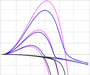
Figure 3 shows by solid lines the dispersion curves $\omega (k)$ for the metal alloy when the Marangoni effect is included, but the wetting energy depends on $h$ only, i.e. the eigenvalues of $\boldsymbol {A}_M$. The dashed lines correspond to the solutions for $s \rightarrow 0$ given by (5.7). Note that the maximum growth rate, $\omega _m$, is only slightly smaller than the one obtained by considering $s \rightarrow 0$ (dashed lines), as expected, since $s$ is fairly small (see table 2). Note that, around the crossing point of the dashed lines ($k \approx k_d$), the degeneracy of the modes $\tilde \omega _h$ and $\tilde \omega _\psi$ is broken for $s>0$ (see figure 3a). Therefore, the mode $1$ (blue line), which for $k< k_d$ can be associated with $\tilde \omega _h$ (magenta dashed line), i.e. the $h$ unstable mode, converts for $k>k_d$ into a mode dominated by the $\psi$-evolution associated with $\tilde \omega _\psi$ (black dashed line). The reverse occurs for mode 2. However, for sufficiently large $k$, mode $1$ departs from both $\tilde \omega _h$ and $\tilde \omega _\psi$, while mode $3$ (solid red line in figure 3b) approaches the asymptotic behaviour of $\tilde \omega _h$.

Figure 3.

Dispersion relations including Marangoni effect and considering wetting energy depending only on thickness ($\tau =0$): (a) zooms into the unstable region (small $k$ values), and (b) shows the results for a larger $k$-range. The solid blue, black and red lines show $\omega _{1,2,3}(k)$, while the dashed lines correspond to the results for $s \rightarrow 0$, $\tilde \omega _h$ (magenta) and $\tilde \omega _\psi$ (grey).

Once the eigenvalues $\omega _i(k)$ ($i=1,2,3$) are obtained, we proceed to calculate the corresponding complex amplitudes of the eigenfunctions

(5.13)\begin{equation} \boldsymbol{X}_i = \left( \begin{array}{@{}c@{}} h_{1i} \\ \varGamma_{1i} \\ \psi_{1i} \end{array} \right),\end{equation}

for each normal mode at a given $k$ (see (4.8)), and $|\boldsymbol {X}_i|^2=h_{1i}^2+\varGamma _{1i}^2+\psi _{1i}^2=1$. Note that, due to the nature of the considered problem, all the amplitudes are, in fact, real numbers with their signs indicating whether $\varGamma _{1i}$ or $\psi _{1i}$ are in-phase or anti-phase with $h_{1i}$. Figure 4 shows the eigenfunctions corresponding to the eigenvalues $\omega _{1,2,3}(k)$ in figure 3. For $k < k_d=0.3689$, figure 4(a) shows that the amplitude of the $h$-eigenfunctions of mode $3$ are negligible with respect to those of modes $1$ and $2$. Instead, in the same $k$-range, figure 4(b) shows that the amplitude of the unstable mode $1$ for $\varGamma$ is very small, while those of modes $2$ and $3$ are much larger. Finally, figure 4(c) shows that the amplitude of the $\psi$-eigenfunction is negligible for mode $3$ in comparison with modes $1$ and $2$. These results illustrate that, for the unstable $k$ range, modes $1$ and $2$ are mainly connected with perturbations in $h$ and $\psi$, respectively, while mode $3$ is more prone to be excited by perturbations in $\varGamma$. These results are in agreement with the previous discussion on the conversion of modes when degeneracy close to $k_d$ is broken for $s>0$. Also, note that the transitions between in-phase and anti-phase behaviour of the $\varGamma _{11}$ and $\psi _{13}$ modes occur at $k_d$.

Figure 4.

Amplitudes of the eigenfunctions including Marangoni effect and considering wetting energy depending only on thickness ($\tau =0$) (dispersion relation shown in figure 3) for (a) $h$, (b) $\varGamma$ and (c) $\psi$. The vertical grey dashed lines indicate the value of $k_d$.

5.2. Nonlinear regime

We proceed by solving numerically the nonlinear (2.11a)–(2.11c); see Appendix B for details. We consider the initial condition corresponding to the monochromatic perturbations of the three fields

(5.14)\begin{equation} \boldsymbol{\varLambda} =\boldsymbol{\varLambda}_0 +\epsilon_1 \boldsymbol{X}_1(k) \, {\rm e}^{{\rm i} k x + \omega_1(k) t},\end{equation}

where $0<\epsilon _1\ll 1$. Here, we use $\epsilon _1=0.01$.

More precisely, we consider a flat uniform film in a spatial domain $0 \leq x \leq \lambda =2 {\rm \pi}/k$ with periodic boundary conditions and initial perturbations as given by (5.14). We take $k=0.25$, so that the corresponding eigenvalue is $\omega _1=0.00395$ (see figure 3). Figure 5(a) shows the corresponding $h$, $\varGamma$, $\psi$ and $\phi$ profiles at different times. We observe the instability development until the film breakup and drop formation. Figure 6 compares the evolution of the perturbations at $x=0$ with the LSA prediction, that is, an exponential growth with the corresponding eigenvalue, $\omega _1$. Interestingly, the exponential growth is valid not only for small perturbations and early times (as expected), but even up to times close to the film breakup (i.e. $h$ approaching $h_\ast$), when the perturbations have increased at least an order of magnitude with respect to their initial values. This result is consistent with similar ones found for other single-phase films, see, e.g. Sharma & Jameel (Reference Sharma and Jameel1993) and Sharma et al. (Reference Sharma, Kishore, Salaniwal and Ruckenstein1995). The departure from the linear model is due to the change of the profiles with respect to the sinusoidal shape as the system approaches the breakup (see figure 3c,d), which requires the excitation of new wavenumbers because of a nonlinear transfer of energy to these new $k$ values (see figure 6(a) for $t>1000$). As a consequence, the evolution of the perturbations with the original wavenumber tends to a plateau, since its energy is depleted to feed the other wavenumbers. Note that $\phi$ and $\varGamma$ become identical for very long times, i.e. when the drop has formed since it constitutes a new equilibrium state.

Figure 5.

Spatial profiles of $h$, $\varGamma$, $\psi$ and $\phi$ at different times obtained from the numerical solution of the nonlinear equations when the flat film is perturbed as in (5.14) with $k=0.25$ only by mode $1$ (with Marangoni effect and wetting energy depending only on thickness ($\tau =0$)). Panels show (a) $t=609$, (b) $t=809$, (c) $t=953$ and (d) $t=1108$.

Figure 6.

Perturbations at $x=0$ as a function of time for a monochromatic ($k=0.25$) perturbation including Marangoni effect and considering wetting energy depending only on thickness ($\tau =0$). Dashed lines correspond to LSA for $h$ (blue), $\varGamma$ (green), $\psi$ (red) and $\phi$ (black): (a) single unstable mode (see (5.14)), (b) all three modes (see (5.16)). Solid lines show the numerical simulation results with the same initial conditions.

Moreover, the LSA can be used to estimate the breakup time as

(5.15)\begin{equation} t_{break}= \frac{1}{\omega_1} \ln \frac{1-h_\ast}{\epsilon_1}, \end{equation}

which yields $t_{break}= 1184$. According to the numerical simulations, this time should be between those shown in figure 5c,d) (i.e. between $t=953$ and $1108$), so that the prediction from LSA gives a reasonable estimate.

Next, we consider the case when all three normal modes are excited

(5.16)\begin{equation} \boldsymbol{\varLambda} =\boldsymbol{\varLambda}_0 +\epsilon_1 \boldsymbol{X}_1(k) \,{\rm e}^{{\rm i} k x + \omega_1(k) t} +\epsilon_2 \boldsymbol{X}_2(k) \, {\rm e}^{{\rm i} k x + \omega_2(k) t}+\epsilon_3 \boldsymbol{X}_3(k)\, {\rm e}^{{\rm i} k x + \omega_3(k) t}, \end{equation}

where $\epsilon _1$, $\epsilon _2$ and $\epsilon _3$ were chosen so as to ensure that the amplitudes of the perturbations in $h$, $\varGamma$ and $\psi$ are initially equal to $0.01$. Figure 6(b) compares the results of this numerical simulation (solid lines) with those of the LSA (dashed lines). We observe that the full problem is also very well described by the LSA, even up to times very close to breakup. Naturally, the evolution is not represented by a straight line (in linear–log scale), since it is a linear combination of three exponential terms.

Before concluding this section, we note that we have also considered a single mode perturbed by a superposition of two wavenumbers, one unstable and one stable (figures not shown for brevity). As expected, the stable wavenumber decays exponentially, while the unstable one grows. In the context of melted metallic thin films, if the duration of the laser pulses (and correspondingly the liquid lifetime) is shorter than the decay time, the subsequent solidification freezes the evolution. Therefore, the stable modes may still appear as an outcome of such experiments.

6. Marangoni effect combined with concentration-dependent wetting energy

Let us now consider the wetting energy, $F$, that depends on both $\varGamma$ and $\phi$ (see (3.16)). This type of dependence yields an additional contribution to matrix $\boldsymbol {A}$, see (4.13), of the form

(6.1)\begin{equation} \boldsymbol{A}=\boldsymbol{A}_M+ k^2 \boldsymbol{A}_1 + k^4 \boldsymbol{A}_2 ,\end{equation}

where

(6.2)$$\begin{gather} \boldsymbol{A}_1 =\frac{\tau K}{2} ({\hat F}^0-{\hat F}^{\prime 0}) \left( \begin{array}{@{}c@{\quad}c@{\quad}c@{}} 3 \varGamma _0 s-2 \phi _0 & 2 s & 2 \\[4pt] 3 \varGamma _0 (2 D+2 \varGamma _0 s-\phi _0) & 3 \varGamma _0 s & 3 \varGamma _0 \\[4pt] \phi _0 (6 D+3 \varGamma _0 s-2 \phi _0) & 2 s \phi _0 & 2 \phi _0 \end{array} \right), \end{gather}$$

(6.3)$$\begin{gather}\boldsymbol{A_2} = \frac{\tau K}{2} s \varGamma_0 {\hat F}^0 \left( \begin{array}{@{}c@{\quad}c@{\quad}c@{}} 2 & 0 & 0 \\[4pt] 3 \varGamma _0 & 0 & 0 \\[4pt] 2 \phi _0 & 0 & 0 \end{array} \right). \end{gather}$$

The additional contributions yield the characteristic equation which generalizes (5.6). Since the equation is rather cumbersome to deal with, we show here just the figures that use the parameters from the melted metal problem. The wetting energy dependence on concentration, i.e. $F(h,\varGamma,\phi )$, is assumed to be given by (3.13).

Let us first consider the case $s\rightarrow 0$. For a given $\tau$, one solution is $\tilde \omega _h$ from (5.2a,b). In this expression, $\tilde k_{c,h}$ is calculated using $F_{hh}^0$ (which depends linearly on $\tau$), but $\hat \gamma _0 =1$ (see (3.10)), since $\tilde \omega _h$ does not include Marangoni effect. Figure 7 represents these solutions for different values of $\tau$ as magenta dashed lines. In this figure, the grey dashed line corresponds to $\tilde \omega _{\psi }$, which is neither affected by the Marangoni effect, nor by the value of $\tau$. Note that the crossings, where there is degeneracy of $\tilde \omega _h (\tau )$ and $\tilde \omega _{\psi }$, give new values of $k_d$ that depend on $\tau$.

Figure 7.

Dispersion relations for modes $1$ (solid blue) and $2$ (solid black) when both Marangoni effect and concentration-dependent wetting energy are considered ($\tau =1$ and $\tau =-0.9$) compared with the case when the wetting energy depends only on $h$ ($\tau =0$) (also shown in figure 3). The magenta dashed lines correspond to $\tilde \omega _h$ and the grey dashed line corresponds to $\tilde \omega _{\psi }$.

Figure 7 also shows the corresponding dispersion relations for modes $1$ (blue) and $2$ (black) for $\tau =1$ and for $\tau =-0.9$ . These results show that the inclusion of the wetting energy dependence on concentrations ($\tau \neq 0$) produces significant changes of the growth rates with respect to $\tau =0$. In particular, we observe that both the critical wavenumber, $k_{c,1}$, and the maximum growth rate, $\omega _m$, increase (decrease) significantly for positive (negative) values of $\tau$. As a consequence, the wavenumber of the maximum growth rate, $k_m$, can fall in the stable range of the $\tau =0$ case for $\tau$ sufficiently large. The physical basis for this behaviour is that $\tau >0$ increases the wetting energy, leading to increased instability of mode $1$, which is dominated by the film thickness evolution. Note that the stable mode $3$ is not shown in figure 7 since it corresponds to much smaller growth rates (see figure 3); the effect of $\tau$ is similar to what is shown in figure 7 for mode $2$.

Figure 8 shows the amplitudes of the eigenfunctions for the eigenvalues shown in figure 7 for $\tau =1$ and $\tau =-0.9$. We note that the amplitudes for $\tau =0$ in figure 4 are qualitatively similar to the ones for $\tau =1$ in figure 8, but the transitions between in-phase and anti-phase behaviour of the $\varGamma _{11}$ and $\psi _{13}$ modes move now to larger $k$ values in consonance with the increase of $k_d (\approx k_c)$. However, there are remarkable differences between $\tau =1$ and $\tau =-0.9$ in $\varGamma$ and $\psi$ for modes $1$ and $2$ . In fact, the comparison of $\varGamma _{12}$ and $\psi _{12}$ between both values of $\tau$ shows that they change sign for small $k$ values (that include the unstable region of mode $1$), while for large $k$ values (stable region) this sign reversal does not occur. In contrast, there is no such sign change of $\varGamma _{11}$ and $\psi _{11}$ for small $k$ values, but there is a sign change for large $k$ values. Note that mode $3$ is the least affected by the value of $\tau$. As mentioned above, the contribution of $h$ perturbations to mode $1$ is predominant in the unstable domain (small $k$ values), as seen by comparing the blue lines with the black and red ones in figure 8(a,d).

Figure 8.

Amplitudes of eigenfunctions when both Marangoni effect and concentration-dependent wetting energy are considered for $\tau = 1.0$ (a–c) and $\tau = -0.9$ (d–f), and for (a,d) $h$, (b,e) $\varGamma$ and (c,f) $\psi$. The vertical grey dashed lines indicate the value of $k_d$.

Figure 9 compares LSA predictions with the nonlinear numerical simulations for the considered values of $\tau$. Here, we perturb the base state by a mode $1$ monochromatic perturbation for $\tau =1$ and $\tau =-0.9$ using $k=0.2$. According to figure 7, this wavenumber corresponds to unstable perturbations. The comparison between figures 6(a), 9 (a) and 9(c) shows a similar qualitative behaviour, except for the fact that the time scales of the breakups change due to the different growth rates as $\tau$ varies (see figure 7). Clearly, the predictions of the LSA remain valid close to the breakup time, which varies as the inverse of the growth rate, $\omega _1$.

Figure 9.

Perturbations at $x=0$ as a function of time for mode $1$ and $k=0.2$ when both Marangoni effect and concentration-dependent wetting energy are considered. Solid lines: $h$ (blue), $\varGamma$ (green), $\psi$ (red) and $\phi$ (black) as given by the numerical simulations for (a) $\tau = 1$ and (b) $\tau = -0.9$. Dashed lines: the LSA predictions. Note different time ranges for (a,b).

7. Summary and conclusions

This paper analyses the stability properties of a binary fluid thin film, focusing on the influence of the solutal Marangoni effects and the fluid–solid interaction, including its dependence on concentrations. The results include a LSA using analytical methods as well as a comparison with the numerical solutions of the full nonlinear problem. Due to the complexity of the task at hand, we have implemented various simplifications and attempted to concentrate on the main aspects of the problem as much as possible.

Carrying out tractable and insightful LSA requires the existence of a stationary base state. We find that such a state is possible when surface and volumetric chemical potentials are balanced, leading to vanishing (to the leading order) fluid exchange between the surface and the volume.

We find it helpful to separate the discussion into two separate cases. The first one focuses on the Marangoni effect assuming a wetting energy $F = F(h)$ (therefore concentration independent). Our finding is that the Marangoni effect alters the critical wavenumber, increasing the unstable $k$-range with respect to the results that do not include Marangoni effects (Diez et al. Reference Diez, González, Garfinkel, Rack, McKeown and Kondic2021). Therefore, the Marangoni effect leads to faster formation of smaller droplets, assuming that the LSA findings extend qualitatively to the nonlinear regime. We note that the previous experiments involving liquid metal nanometric films involve a set of parameters that allow for modelling of the problem accurately by assuming a very thin adsorption interface, which corresponds to the limit $s \rightarrow 0$ ($a_s \ll h_0$), and leads to simple analytical expressions for the growth rates. In the context of flows such that surfactants are relevant, we note that a case with surfactant and a certain surface tension compared with another without surfactant and the same surface tension (red dashed line in figure 3a) shows no change in $k_{c,h}$, but a slight decrease of the maximum growth rate.

Notably, comparing the LSA results with the numerical simulations of the full nonlinear problem reveals that most of the evolution is well described by the LSA results, with a significant difference between LSA and nonlinear simulations only very close to the film breakup time. Consequently, the validity of the linear approach can be extended to rather large unstable perturbations, confirming the LSA predictions regarding the expected size of the resulting drops and their formation times. We have made this comparison not only for single mode and monochromatic perturbations but also for a combination of modes and multiple wavenumbers. These combinations, which require a precise understanding of the stable modes, are relevant for the transient initial stages of the instability. In fact, this transient behaviour may be of particular interest in the case of melted metallic films, since they could re-solidify and freeze the evolution before reaching the long-time asymptotic behaviour dominated by the unstable mode.

When additional dependence of the wetting energy on both surface and bulk concentrations is considered, we can describe its influence in terms of a single parameter, $\tau$. As $\tau$ increases, both the critical wavenumber and the maximum growth rate of the unstable mode increase. While the Marangoni effect is found to be always destabilizing, the influence of concentration dependence of the wetting energy on concentrations could be either stabilizing ($\tau <0$) or destabilizing ($\tau >0$), compared with the $\tau =0$ case. Therefore, the manner in which instability develops depends on the material properties of the considered fluids. For the considered case (including the wetting energy dependence on concentration), we have also confirmed an excellent agreement of the LSA results with the nonlinear numerical simulations until times close to film breakup.

Several aspects deserve future study. In this paper, we have selected particular forms of $G(\phi )$ and $G_s(\varGamma )$ that preclude the existence of additional unstable modes, since both are convex functions of their argument. However, one could also consider potentials that include concavity due to additional quadratic terms to an entropic or double-well potential. This could lead to new unstable modes with much larger growth rates (at also much larger wavenumber), as considered in Diez et al. (Reference Diez, González, Garfinkel, Rack, McKeown and Kondic2021) for the case without the Marangoni effect and without consideration of concentration-dependent wetting energies, but with double-well potential. Therefore, an interesting extension of our analysis could be the inclusion of these types of potentials. A more involved aspect of the problem is the possibility that the base state is non-stationary, which occurs when the flux $\boldsymbol {J_0} \neq 0$. Considering these issues may allow for a better understanding of some features of experimentally observed results, such as core–shell and Janus-like droplets in the experiments carried out with liquid metals. We expect that our work provides a basic set-up that can serve as a basis for such endeavours.