1 Introduction
Most wall surfaces encountered in geophysical and engineering flows cannot be regarded as hydraulically smooth. Vegetated and urban canopies and natural river beds are considered rough walls (Raupach Reference Raupach1994b ; Finnigan Reference Finnigan2000; Cheng & Castro Reference Cheng and Castro2002), and the wall roughness is inevitably generated in production processes owing to the imperfections of surface finishing. Furthermore, erosion or corrosion by aging and by organic or inorganic fouling processes make the surfaces rough, which is well known to cause a significant rise in skin friction, especially for high-Reynolds-number turbulent flows (Wahl Reference Wahl1989; Bons et al. Reference Bons, Taylor, McClain and Rivir2001; Langelandsvik, Kunkel & Smits Reference Langelandsvik, Kunkel and Smits2008; Kirschner & Brennan Reference Kirschner and Brennan2012). This causes a serious decrement in the performance of turbomachinery (Acharya, Bornstein & Escudier Reference Acharya, Bornstein and Escudier1986; Bons Reference Bons2010), and in the case of the roughness of a ship’s hull it substantially increases fuel consumption (Townsin Reference Townsin2003; Schultz et al. Reference Schultz, Bendick, Holm and Hertel2011). It is thus crucial to estimate the rise in skin friction in mechanical, marine and aerospace engineering.
Wall roughness usually gives rise to significant skin friction, which increases turbulent flows and leads to a downward shift of the mean velocity profile that is referred to as the roughness function (Hama Reference Hama1954; Schlichting et al. Reference Schlichting, Gersten, Krause, Oertel and Mayes1955). The pioneering work on the skin friction coefficient in rough-wall turbulence was performed by Nikuradse (Reference Nikuradse1933). His large number of measurements of a pressure drop in pipes with walls covered by sand grains revealed that the skin friction coefficient only depended on an equivalent sand grain roughness in the sufficiently high-Reynolds-number regime (fully rough). Further extensions of this work were performed by Colebrook et al. (Reference Colebrook, Blench, Chatley, Essex, Finniecome, Lacey, Williamson and MacDonald1939), who investigated the skin friction coefficient for several industrial pipes. Moody (Reference Moody1944) consolidated those data as a Moody chart for practical engineering applications. The Moody chart is certainly a powerful tool for estimating pressure loss by the wall roughness as long as the equivalent roughness for the roughness of interest is known a priori, such as that of commercial steel pipes, glass and concrete. However, in terms of naturally occurring roughness due to erosion, corrosion or fouling processes, the equivalent roughness is usually unknown. Hence, to estimate the equivalent roughness to predict the skin friction, many studies have dedicated their efforts to exploring the relation between equivalent roughness and roughness topology (Schlichting et al. Reference Schlichting, Gersten, Krause, Oertel and Mayes1955; Dvorak Reference Dvorak1969; Dirling Reference Dirling1973; Coleman, Hodge & Taylor Reference Coleman, Hodge and Taylor1984; Sigal & Danberg Reference Sigal and Danberg1990; Van Rij et al. Reference Jennifer, Belnap and Ligrani2002).
For estimation of the equivalent roughness, Dirling (Reference Dirling1973) proposed a roughness parameter including a roughness density and a shape parameter. The roughness density was represented as the ratio of the average element spacing to roughness height, while the shape parameter accounted for the frontal area and the windward wetted surface area of a single roughness element. In order to extend the applicability of the roughness parameter of Dirling (Reference Dirling1973), Sigal & Danberg (Reference Sigal and Danberg1990) replaced the roughness density with the ratio of the area of the smooth surface before adding the roughness and the total frontal area over the rough surface. Van Rij et al. (Reference Jennifer, Belnap and Ligrani2002) proposed a more generalized form by replacing the shape parameter of Dirling (Reference Dirling1973) with the ratio of the total frontal area to the total wetted area for all the roughness elements, and reported that the proposed correlation could also be applicable to walls with non-uniform, three-dimensional roughness with irregular geometry and arrangement. Furthermore, this correlation was reported to provide a good estimation for real turbine blade roughness (Bons Reference Bons2002). Similar to the idea of Acharya et al. (Reference Acharya, Bornstein and Escudier1986), Sigal & Danberg (Reference Sigal and Danberg1990) and Bons (Reference Bons2005) introduced a parameter representing the forward-facing surface angle of the roughness elevation, and demonstrated the effectiveness of the parameter for characterizing real rough surfaces.
Other types of correlations for the equivalent roughness based on statistical moments of surface elevation have been explored (Musker Reference Musker1980; Townsin et al.
Reference Townsin, Byrne, Svensen and Milne1981; Flack & Schultz Reference Flack and Schultz2010; Flack et al.
Reference Flack, Schultz, Barros and Kim2016). Musker (Reference Musker1980) proposed a correlation function for the equivalent roughness for hull roughness using the standard deviation, skewness and kurtosis of the probability density function of the surface elevation. Flack & Schultz (Reference Flack and Schultz2010) stated that the standard deviation and the skewness were particularly effective parameters for describing a surface hydraulically, and proposed a correlation function including the standard deviation and the skewness. Their proposed correlation function, optimized by using experimental data for a large number of irregular rough walls, indicated that positive skewness increased the equivalent roughness. However, their correlation function was only valid for rough walls whose skewness was greater than 1.0. For application to rough surfaces with significantly negative skewness, Flack et al. (Reference Flack, Schultz, Barros and Kim2016) developed a correlation for grit-blasted rough walls whose skewness ranged from
 $-1.5$
to 0.66. Their correlation function implied that negative skewness increased the equivalent roughness, which was however in contrast to the proposition made by Flack & Schultz (Reference Flack and Schultz2010). They also mentioned that, to reveal what/how roughness characteristics affected the equivalent roughness, a systematic study of the relation between the roughness characteristics and the equivalent roughness was essentially required.
Numerical simulation, on the other hand, has been recognized as a very powerful tool for discussing fundamental flow physics inside the roughness sublayer and to systematically investigate the effects of roughness topological parameters on turbulence. Accordingly, direct numerical simulation (DNS) or large-eddy simulation (LES) for flows over spanwise extended transverse ribs (Miyake, Tsujimoto & Nakaji Reference Miyake, Tsujimoto and Nakaji2001; Leonardi et al. Reference Leonardi, Orlandi, Smalley, Djenidi and Antonia2003; Ashrafian, Andersson & Manhart Reference Ashrafian, Andersson and Manhart2004; Nagano, Hattori & Houra Reference Nagano, Hattori and Houra2004; Ikeda & Durbin Reference Ikeda and Durbin2007; Jin, Uth & Herwig Reference Jin, Uth and Herwig2015) and three-dimensional roughness with regular arrangement (Bhaganagar, Kim & Coleman Reference Bhaganagar, Kim and Coleman2004; Orlandi & Leonardi Reference Orlandi and Leonardi2008; Lee, Sung & Krogstad Reference Lee, Sung and Krogstad2011; Chatzikyriakou et al. Reference Chatzikyriakou, Buongiorno, Caviezel and Lakehal2015; Kuwata & Suga Reference Kuwata and Suga2016b ,Reference Kuwata and Suga c ) have been performed.
Orlandi & Leonardi (Reference Orlandi and Leonardi2008) carried out DNS of turbulence over cubes, cylinders, transverse wedges and longitudinal wedges with staggered arrangement to explore a new parametrization for turbulence over regularly distributed rough walls. They found a proportionality between the root-mean-square of the wall-normal Reynolds stress at the roughness peak and the roughness function. Further discussions were made by Orlandi (Reference Orlandi2013). They stressed that the wall-normal Reynolds stress could be used to parametrize turbulence structures, and demonstrated the possibility of a derivation of a new kind of Moody diagram.
Fortunately, modern computer technology enables us to perform DNS of turbulence over rough surfaces with complex geometries, including irregular/random roughness (Napoli, Armenio & De Marchis Reference Napoli, Armenio and De Marchis2008; De Marchis, Napoli & Armenio Reference De Marchis, Napoli and Armenio2010; Cardillo et al. Reference Cardillo, Chen, Araya, Newman, Jansen and Castillo2013; Yuan & Piomelli Reference Yuan and Piomelli2014; Bhaganagar & Chau Reference Bhaganagar and Chau2015; Forooghi et al. Reference Forooghi, Stroh, Magagnato, Jakirlić and Frohnapfel2017, Reference Forooghi, Stroh, Schlatter and Frohnapfel2018a ) or scanned real surfaces (Busse, Lützner & Sandham Reference Busse, Lützner and Sandham2015; Busse, Thakkar & Sandham Reference Busse, Thakkar and Sandham2017; Forooghi et al. Reference Forooghi, Weidenlener, Magagnato, Böhm, Kubach, Koch and Frohnapfel2018b )
Napoli et al. (Reference Napoli, Armenio and De Marchis2008) considered two-dimensional irregular corrugated walls to discuss the influence of surface slope on turbulence. In their study, the roughness function for the rough surfaces with an effective slope lower than a certain threshold increased with the effective slope. However, the dependence on the effective slope got weaker for rough surfaces with effective slopes higher than the threshold. The dependence of turbulence on the effective slope has also been confirmed by experiments (Schultz & Flack Reference Schultz and Flack2009) and systematic DNS studies on systematically varied sinusoidal wavy wall pipes (Chan et al. Reference Chan, MacDonald, Chung, Hutchins and Ooi2015) and surfaces with randomly distributed semi-ellipsoid/cone roughness (Forooghi et al. Reference Forooghi, Stroh, Magagnato, Jakirlić and Frohnapfel2017). Chan et al. (Reference Chan, MacDonald, Chung, Hutchins and Ooi2015) additionally suggested the importance of the absolute values of the roughness height amplitude to scale the roughness function as well as the effective slope. The systematic DNS study on the influence of the solidity, which is comparable to the effective slope (Napoli et al. Reference Napoli, Armenio and De Marchis2008; Thakkar, Busse & Sandham Reference Thakkar, Busse and Sandham2017), on turbulence was conducted by MacDonald et al. (Reference MacDonald, Chan, Chung, Hutchins and Ooi2016). Their DNS results of turbulence over three-dimensional transitionally rough sinusoidal surfaces suggested that an increase in the solidity increased the roughness function in the sparse regime of roughness but decreased in the dense regime. They also analysed the integrated mean momentum balance and reached a conclusion that the decrease in the roughness function in the dense regime was due to a reduction in the Reynolds shear stress.
In terms of the statistical moments, Bhaganagar & Chau (Reference Bhaganagar and Chau2015) found from their DNS results on turbulence over three-dimensional irregular rough surfaces that the skewness and the kurtosis could be effective for characterizing the roughness function although the spacing between the roughness elements was not sensitive to the roughness function for irregular rough walls. The importance of the skewness has also been reported by DNS studies on surfaces with randomly distributed semi-ellipsoid/cone roughness (Forooghi et al. Reference Forooghi, Stroh, Magagnato, Jakirlić and Frohnapfel2017) and realistic rough surfaces (Yuan & Piomelli Reference Yuan and Piomelli2014). Note, however, that they also stressed the importance of the effective slope (Napoli et al. Reference Napoli, Armenio and De Marchis2008). Indeed, Yuan & Piomelli (Reference Yuan and Piomelli2014) stated that, as the statistical moments did not contain information regarding the rough-surface slope, the statistical moments were not suitable for the wavy roughness. Recently, Thakkar et al. (Reference Thakkar, Busse and Sandham2017) performed a large number of DNS studies for irregular real surfaces in order to relate surface characteristics to the roughness function in the transitionally rough regime. They found that the streamwise correlation length non-dimensionalized by the mean peak-to-valley height was significantly effective as well as the known parameters of the solidity, skewness and the root-mean-square roughness. Forooghi et al. (Reference Forooghi, Stroh, Magagnato, Jakirlić and Frohnapfel2017) suggested using the roughness parameter to characterize the equivalent roughness based on DNS results of systematically varied roughness at fixed values of the root-mean-square roughness, skewness, kurtosis and effective slope. They suggested that the peak size distribution could independently influence the equivalent roughness, in addition to the peak-to-valley roughness, skewness and effective slope.
Many other important numerical/experimental studies on turbulence over rough walls can be found in the literature, and a great deal of effort has been made to examine the relation between roughness topological parameters and increase in skin friction. However, detailed mechanisms describing the increase in skin friction have not been proposed despite the fact that roughness induces many dynamical effects, namely, velocity dispersion, turbulence, and pressure and viscous drags. Therefore, in the present study, to better understand the mechanisms of skin friction modification due to the change in two important roughness parameters, i.e. the root-mean-square roughness and the skewness, we mathematically discuss the mechanisms of skin friction modification by performing DNS of turbulence over systematically varied irregular rough surfaces. The dynamical effects that contribute to an increase in the skin friction coefficient are discussed by analysing the integrated spatial and Reynolds- (double-) averaged Navier–Stokes equation. Moreover, using the recent DNS and experimental data, including the present results, the present study attempts improvement of the correlation function for the equivalent roughness based on the statistical moments (Flack & Schultz Reference Flack and Schultz2010). It should be remarked, however, that this study does not intend to explore a universal correlation for the equivalent roughness because the available DNS and experimental data are not sufficient to comprehensively examine the influence of the roughness parameters on the equivalent roughness.
2 Numerical approach
Owing to the simplicity of the curved boundary wall treatment, the lattice Boltzmann method (LBM) has achieved considerable success in complex flow simulations (e.g. Hatiboglu & Babadagli Reference Hatiboglu and Babadagli2008; Suga et al. Reference Suga, Tanaka, Nishio and Murata2009; Suga & Nishio Reference Suga and Nishio2009; Beugre et al. Reference Beugre, Sbastien, Grard, Michel, Dominique and Pierre2010; Parmigiani et al. Reference Parmigiani, Huber, Bachmann and Chopard2011; Chukwudozie & Tyagi Reference Chukwudozie and Tyagi2013). In particular, as the LBM algorithm inherently has high spatial and temporal locality, it is ideal in massive parallel computing using the message passing interface (MPI) and graphics processing units (GPUs) as reported by Xipeng et al. (Reference Xipeng, Yun, Xiaowei and Wei2013) and Huang et al. (Reference Huang, Shi, He and Chai2015). Additionally, the nature of its low numerical dissipation and dispersion leads to success in DNS of fundamental turbulent flows (e.g. Lammers et al. Reference Lammers, Beronov, Volkert, Brenner and Durst2006; Chikatamarla et al. Reference Chikatamarla, Frouzakis, Karlin, Tomboulides and Boulouchos2010; Bespalko, Pollard & Uddin Reference Bespalko, Pollard and Uddin2012; Suga et al. Reference Suga, Kuwata, Takashima and Chikasue2015; Fattahi et al. Reference Fattahi, Waluga, Wohlmuth, Rüde, Manhart and Helmig2016; Wang, Wang & Guo Reference Wang, Wang and Guo2016; Gehrke, Janßen & Rung Reference Gehrke, Janßen and Rung2017). The above-mentioned advantages enable us to apply the LBM to various complex turbulent flow problems such as flows around porous media (e.g. Hasert, Bernsdorf & Roller Reference Hasert, Bernsdorf and Roller2011; Krafczyk et al. Reference Krafczyk, Kucher, Wang and Geier2015; Kuwata & Suga Reference Kuwata and Suga2015b , Reference Kuwata and Suga2016b ,Reference Kuwata and Suga c , Reference Kuwata and Suga2017) or around rough walls (e.g. Jin et al. Reference Jin, Uth and Herwig2015; Tóth & Jánosi Reference Tóth and Jánosi2015).
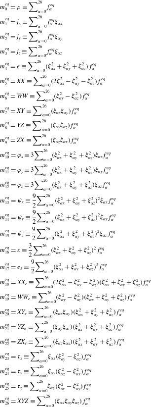
Parameters of the D3Q27 discrete velocity model.

The lattice Boltzmann equation can be obtained by discretizing the velocity space of the Boltzmann equation into a finite number of discrete velocities
 $\unicode[STIX]{x1D743}_{\unicode[STIX]{x1D6FC}}~\{\unicode[STIX]{x1D6FC}=0,\ldots ,Q-1\}$
. There are several discrete velocity models for three-dimensional flow simulations, such as the D3Q15, D3Q19 and D3Q27 models. It was reported that, although unphysical spurious currents were sometimes visible in the D3Q15 and D3Q19 models in axisymmetric flows, they were effectively suppressed by the D3Q27 model (White & Chong Reference White and Chong2011; Kang & Hassan Reference Kang and Hassan2013; Kuwata & Suga Reference Kuwata and Suga2015a
). Furthermore, to ensure numerical stability for high-Reynolds-number flows, it is effective to apply the multiple-relaxation-time (MRT) scheme (d’Humiéres et al.
Reference d’Humiéres, Ginzburg, Krafczyk, Lallemand and Luo2002). Accordingly, the present study employs the D3Q27 MRT-LBM of Suga et al. (Reference Suga, Kuwata, Takashima and Chikasue2015). The time evolution of the distribution function of the MRT-LBM can be written as
 $$\begin{eqnarray}|\,\boldsymbol{f}(\boldsymbol{x}+\unicode[STIX]{x1D743}_{\unicode[STIX]{x1D6FC}}\unicode[STIX]{x1D6FF}t,t+\unicode[STIX]{x1D6FF}t)\!\rangle -|\,\boldsymbol{f}(\boldsymbol{x},t)\!\rangle =-\boldsymbol{M}^{-1}\hat{\unicode[STIX]{x1D64E}}[|\boldsymbol{m}(\boldsymbol{x},t)\!\rangle -|\boldsymbol{m}^{eq}(\boldsymbol{x},t)\!\rangle ],\end{eqnarray}$$
where
 $|\,\boldsymbol{f}\!\rangle$
is
 $|\,\boldsymbol{f}\!\rangle =(f_{0},f_{1},\ldots ,f_{Q-1})^{\text{T}}$
and
 $\unicode[STIX]{x1D6FF}t$
is the time step. Note that for the D3Q27 model,
 $Q=27$
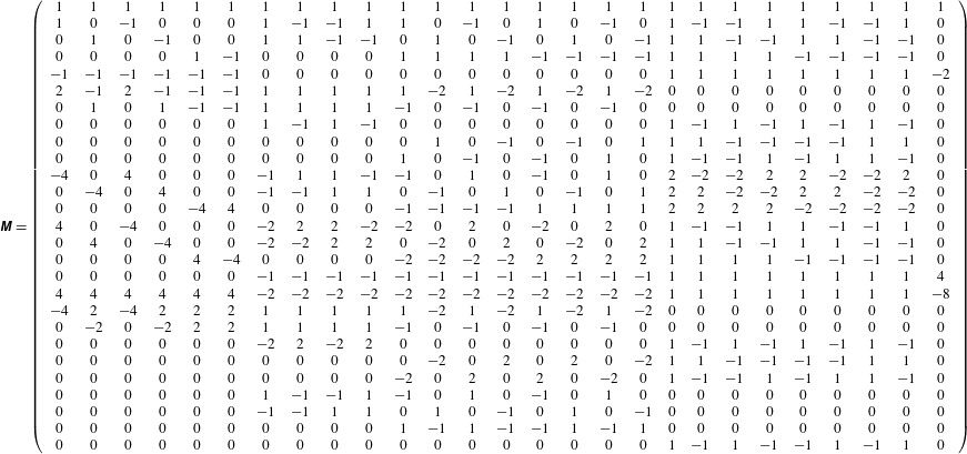
. The parameters for the D3Q27 model are listed in table 1. The matrix
 $\unicode[STIX]{x1D648}$
is a
 $Q\times Q$
matrix that linearly transforms the distribution functions to the moments as
 $|\boldsymbol{m}\!\rangle =\boldsymbol{M}|\,\boldsymbol{f}\!\rangle$
. The equilibrium moment
 $\boldsymbol{m}^{eq}$
is obtained as
 $|\boldsymbol{m}^{eq}\!\rangle =\boldsymbol{M}|\,\boldsymbol{f}^{eq}\!\rangle$
with
 $$\begin{eqnarray}f_{\unicode[STIX]{x1D6FC}}^{eq}=w_{\unicode[STIX]{x1D6FC}}\left(\unicode[STIX]{x1D70C}+\unicode[STIX]{x1D70C}_{0}\left[\frac{\unicode[STIX]{x1D743}_{\unicode[STIX]{x1D6FC}}\boldsymbol{\cdot }\boldsymbol{u}}{c_{s}^{2}}+\frac{(\unicode[STIX]{x1D743}_{\unicode[STIX]{x1D6FC}}\boldsymbol{\cdot }\boldsymbol{u})^{2}-c_{s}^{2}|\boldsymbol{u}|^{2}}{2c_{s}^{4}}\right]\right),\end{eqnarray}$$
where
 $\boldsymbol{u}$
is the fluid velocity and
 $\unicode[STIX]{x1D70C}$
is expressed as the sum of constant and fluctuation terms:
 $\unicode[STIX]{x1D70C}=\unicode[STIX]{x1D70C}_{0}+\unicode[STIX]{x1D6FF}\unicode[STIX]{x1D70C}$
(He & Luo Reference He and Luo1997). The sound speed is
 $c_{s}/c=1/\sqrt{3}$
with
 $c=\unicode[STIX]{x1D6E5}/\unicode[STIX]{x1D6FF}t$
, where
 $\unicode[STIX]{x1D6E5}$
is the lattice spacing and the values of
 $w_{\unicode[STIX]{x1D6FC}}$
are listed in table 1. The equilibrium moments and the transformation matrix are shown in tables 2 and 3, respectively. The collision matrix
 $\hat{\unicode[STIX]{x1D64E}}$
is diagonal:
 $$\begin{eqnarray}\displaystyle \hat{\unicode[STIX]{x1D64E}} & \equiv & \displaystyle \text{diag}(\!0,0,0,0,s_{4},s_{5},s_{5},s_{7},s_{7},s_{7},s_{10},s_{10},s_{10},s_{13},s_{13},\nonumber\\ \displaystyle & & \displaystyle \quad s_{13},s_{16},s_{17},s_{18},s_{18},s_{20},s_{20},s_{20},s_{23},s_{23},s_{23},s_{26}\! ).\end{eqnarray}$$
A set of relaxation parameters presently used is
 $$\begin{eqnarray}\left.\begin{array}{@{}c@{}}s_{4}=1.54,\quad s_{5}=s_{7},\quad s_{10}=1.5,\quad s_{13}=1.83,\quad s_{16}=1.4,\\ s_{17}=1.61,\quad s_{18}=s_{20}=1.98,\quad s_{23}=s_{26}=1.74.\end{array}\right\}\end{eqnarray}$$
The relaxation parameters
 $s_{5}$
and
 $s_{7}$
are related to the kinematic viscosity
 $\unicode[STIX]{x1D708}$
:
 $$\begin{eqnarray}\unicode[STIX]{x1D708}=c_{s}^{2}\left(\frac{1}{s_{5}}-\frac{1}{2}\right)\unicode[STIX]{x1D6FF}t=c_{s}^{2}\left(\frac{1}{s_{7}}-\frac{1}{2}\right)\unicode[STIX]{x1D6FF}t.\end{eqnarray}$$
The presently applied scheme of the D3Q27 MRT-LBM was validated in the application to the DNS of the turbulent channel flow at
 $Re_{\unicode[STIX]{x1D70F}}=180$
. The turbulence statistics including the higher-order turbulence correlations such as the budget terms of the turbulence energy equation and the predicted energy spectra showed almost perfect agreement with those by the spectrum method of Kim, Moin & Moser (Reference Kim, Moin and Moser1987) (see Suga et al.
Reference Suga, Kuwata, Takashima and Chikasue2015).
Equilibrium moments. Here:
 $\unicode[STIX]{x1D70C}$
, density;
 $j_{x},j_{y},j_{z}$
, momenta;
 $e$
, kinetic energy;
 $XX,WW,XY,YZ,ZX$
, second-order tensors;
 $\unicode[STIX]{x1D711}_{x},\unicode[STIX]{x1D711}_{y},\unicode[STIX]{x1D711}_{z}$
, fluxes of the energy;
 $\unicode[STIX]{x1D713}_{x},\unicode[STIX]{x1D713}_{y},\unicode[STIX]{x1D713}_{z}$
, fluxes of the square of the energy;
 $\unicode[STIX]{x1D700}$
, square of the energy;
 $e_{3}$
, cube of the energy;
 $XX_{e},WW_{e}$
, product of
 $XX$
and
 $WW$
by the energy;
 $XY_{e},YZ_{e},ZX_{e}$
, extra-diagonal second-order moments of the energy;
 $\unicode[STIX]{x1D70F}_{x},\unicode[STIX]{x1D70F}_{y},\unicode[STIX]{x1D70F}_{z}$
, third-order pseudo-vectors;
 $XYZ$
, third-order totally antisymmetric tensor.

The
 $27\times 27$
transformation matrix.

3 Flow conditions
Lattice Boltzmann DNS of turbulent open-channel flows over rough surfaces at friction Reynolds number
 $600$
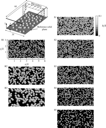
as illustrated in figure 1 are performed. The rough surfaces are generated by randomly distributing hemispheres on a reference solid plane allowing meddling among hemispheres. Simulated rough surfaces coloured by the wall-normal location are shown in figure 1.
Computational geometry and simulated rough surfaces.

To perform simulations over various rough surfaces with practical computational cost, we consider a turbulent open-channel flow system in which we apply the slip boundary condition to the top boundary surface. The turbulence structure near the slip boundary is naturally different from that in a channel centre; however, the present study focuses on turbulence modification near the wall roughness; the main conclusion of the present study is expected to be independent of the choice of the flow type. Periodic boundary conditions are applied to the streamwise and spanwise directions, and flows are driven by imposing a pressure difference between the inlet and outlet boundary faces. To impose the no-slip boundary condition to curved boundary surfaces, we apply a linear interpolated bounce-back scheme which can satisfy second-order spatial accuracy. The computational domain size
 $L_{x}\times L_{y}\times L_{z}$
is set to
 $6.0\unicode[STIX]{x1D6FF}(x)\times \unicode[STIX]{x1D6FF}(y)\times 3.0\unicode[STIX]{x1D6FF}(z)$
. The domain size is validated by comparing the skin friction coefficient with that obtained in the simulation with the larger domain of
 $9.0\unicode[STIX]{x1D6FF}(x)\times \unicode[STIX]{x1D6FF}(y)\times 4.5\unicode[STIX]{x1D6FF}(z)$
. We confirm that the relative difference in the skin friction coefficient is within 0.3 %. Moreover, to check the validity of the computational domain size, we compute the two-point spatial correlation function of the streamwise velocity fluctuations just above the roughness peak, and we confirm that the convergence magnitude values of the streamwise and spanwise correlation functions are within 0.02. Therefore, the present computational domain is expected to be sufficient for precisely reproducing turbulent flows near rough surfaces.
The regular grid domain of
 $2015(x)\times 116(y)\times 1007(z)$
is allocated near the rough surface of
 $y/\unicode[STIX]{x1D6FF}<0.35$
while the twice coarser grid domain of
 $1008(x)\times 112(y)\times 504(z)$
is allocated to the other region of
 $y/\unicode[STIX]{x1D6FF}>0.35$
with an imbalance-correction grid refinement method of Kuwata & Suga (Reference Kuwata and Suga2016a
). The grid resolution near the rough surfaces is 1.9 wall units, which is comparable to that in other lattice Boltzmann DNS studies (Lammers et al.
Reference Lammers, Beronov, Volkert, Brenner and Durst2006; Kuwata & Suga Reference Kuwata and Suga2016b
,Reference Kuwata and Suga
c
, Reference Kuwata and Suga2017; Gehrke et al.
Reference Gehrke, Janßen and Rung2017). At least
 $30(x)\times 30(y)\times 30(x)$
grid points are used to resolve each hemisphere. To validate the grid resolution, a grid independence test is performed by comparing the skin friction coefficient with that obtained by the simulation with a 1.5 times denser mesh, and we confirm that the difference is within 0.04 %.
The friction Reynolds number is based on the averaged friction velocity
 $u_{\unicode[STIX]{x1D70F}}$
and the effective channel height
 $\unicode[STIX]{x1D6FF}_{e}$
defined as
 $$\begin{eqnarray}\unicode[STIX]{x1D6FF}_{e}=\int _{0}^{\unicode[STIX]{x1D6FF}}\unicode[STIX]{x1D711}\,\text{d}y,\end{eqnarray}$$
where
 $\unicode[STIX]{x1D711}$
stands for the
 $x$
–
 $z$
plane porosity defined as the ratio of the
 $x$
–
 $z$
plane area
 $S$
and the
 $x$
–
 $z$
plane area occupied by the fluid phase
 $S_{f}$
:
 $\unicode[STIX]{x1D711}=S_{f}/S$
. The plane porosity is thus a function of the wall-normal coordinate, and varies from 0 (no fluid phase in a certain
 $x$
–
 $z$
plane) to 1 (no solid phase in a certain
 $x$
–
 $z$
plane). Note that the origin of the wall-normal coordinates
 $y=0$
is set on the reference solid plane as shown in figure 1. The averaged friction velocity is computed by the balance between the pressure drop
 $\unicode[STIX]{x0394}P$
and the averaged wall shear stress on the rough surface,
 $\unicode[STIX]{x1D70F}_{w}=\unicode[STIX]{x1D70C}u_{\unicode[STIX]{x1D70F}}^{2}$
, as
 $$\begin{eqnarray}S_{yz}\unicode[STIX]{x0394}P=L_{x}L_{z}\unicode[STIX]{x1D70F}_{w},\end{eqnarray}$$
where
 $S_{yz}$
is the effective cross-sectional area expressed as
 $S_{yz}=L_{z}\unicode[STIX]{x1D6FF}_{e}$
. Thus,
 $u_{\unicode[STIX]{x1D70F}}$
is given as
 $$\begin{eqnarray}u_{\unicode[STIX]{x1D70F}}=\left(\frac{\unicode[STIX]{x0394}P}{\unicode[STIX]{x1D70C}}\frac{\unicode[STIX]{x1D6FF}_{e}}{L_{x}}\right)^{0.5}.\end{eqnarray}$$
In the following, the value with the superscript ‘
 $(\,)^{+}$
’ indicates the value normalized by the averaged friction velocity
 $u_{\unicode[STIX]{x1D70F}}$
and the kinematic viscosity
 $\unicode[STIX]{x1D708}$
. To obtain turbulence statistics, the Reynolds averaging is performed over time for
 $70\unicode[STIX]{x1D6FF}_{e}/u_{\unicode[STIX]{x1D70F}}$
after the flows have reached fully developed states.
4 Rough walls
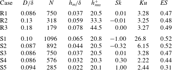
The rough surfaces considered in the present study are generated by randomly distributing a uniform size of hemispheres on a reference solid plane allowing meddling among hemispheres. By changing the number of the hemispheres
 $N$
and their diameter
 $D$
, statistical moments of the roughness elevation such as the mean height
 $h_{m}$
, the standard deviation
 $h_{rms}$
, the skewness
 $Sk$
and the kurtosis
 $Ku$
defined as
 $$\begin{eqnarray}\displaystyle & \displaystyle h_{m}=\frac{1}{L_{x}L_{z}}\iint h\,\text{d}x\,\text{d}z, & \displaystyle\end{eqnarray}$$
 $$\begin{eqnarray}\displaystyle & \displaystyle h_{rms}^{2}=\frac{1}{L_{x}L_{z}}\iint \left(h-h_{m}\right)^{2}\,\text{d}x\,\text{d}z, & \displaystyle\end{eqnarray}$$
 $$\begin{eqnarray}\displaystyle & \displaystyle Sk=\frac{1}{h_{rms}^{3}L_{x}L_{z}}\iint \left(h-h_{m}\right)^{3}\,\text{d}x\,\text{d}z, & \displaystyle\end{eqnarray}$$
 $$\begin{eqnarray}\displaystyle & \displaystyle Ku=\frac{1}{h_{rms}^{4}L_{x}L_{z}}\iint \left(h-h_{m}\right)^{4}\,\text{d}x\,\text{d}z, & \displaystyle\end{eqnarray}$$
are varied. Here,
 $h$
represents rough-surface elevation from the bottom solid wall. The importance of these parameters has been reported (Musker Reference Musker1980; Flack & Schultz Reference Flack and Schultz2010; Flack et al.
Reference Flack, Schultz, Barros and Kim2016; Forooghi et al.
Reference Forooghi, Stroh, Magagnato, Jakirlić and Frohnapfel2017). On the other hand, as reported by many studies (Napoli et al.
Reference Napoli, Armenio and De Marchis2008; Schultz & Flack Reference Schultz and Flack2009; De Marchis et al.
Reference De Marchis, Napoli and Armenio2010; Yuan & Piomelli Reference Yuan and Piomelli2014; Chan et al.
Reference Chan, MacDonald, Chung, Hutchins and Ooi2015; Forooghi et al.
Reference Forooghi, Stroh, Magagnato, Jakirlić and Frohnapfel2017), one of the other important topological characteristics that we should take into account is the slope of the roughness corrugation, which is quantified as the effective slope (
 $ES$
) and is defined as follows:
 $$\begin{eqnarray}ES=\frac{1}{L_{x}}\int \left|\frac{\unicode[STIX]{x2202}h}{\unicode[STIX]{x2202}x}\right|\,\text{d}x.\end{eqnarray}$$
Through systematic investigations for surfaces with three-dimensional pyramid roughness, Schultz & Flack (Reference Schultz and Flack2009) reported that the roughness function linearly increased with
 $ES$
in wavy surfaces where the
 $ES$
value was lower than the threshold value of
 $ES=0.35$
. However, as a focus on the present study is the influence of two parameters, namely
 $h_{rms}$
and
 $Sk$
, on turbulence, the rough surfaces in the present study are confined to surfaces whose effective slope dependence is expected to be small (
 $ES>0.35$
).
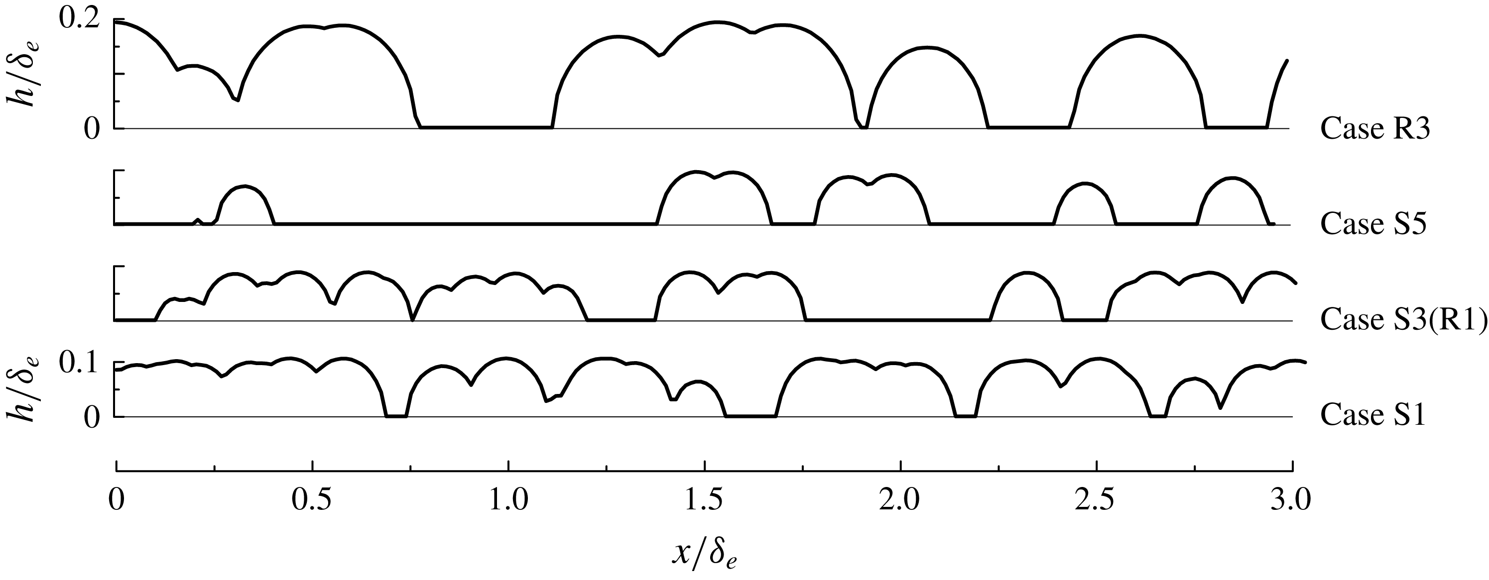
Rough-surface height profiles in cases S1, S3(R1), S5 and R3.

To systematically examine the influence of
 $h_{rms}$
and
 $Sk$
, we generate the first series of rough surfaces of cases R1–R3 whose
 $h_{rms}^{+}$
are varied (from 20 to 45) keeping
 $Sk$
as a constant value of
 $Sk\approx 0.0$
. The second series of rough surfaces are cases S1–S5 whose
 $Sk$
are varied in a wide range from negative to positive values (from
 $-1.0$
to +1.0) keeping
 $h_{rms}^{+}$
as a constant value of
 $h_{rms}^{+}\approx 21$
. (Note that the rough-wall cases R1 and S3 are identical.) Snapshots of the generated rough surfaces coloured by the wall-normal location are depicted in figure 1, and the rough-surface height profiles are depicted in figure 2. The controlling parameters for the roughness generation (
 $D,N$
) and the resultant roughness parameters (
 $h_{m},Sk,Ku,ES$
) are listed in table 4. The first series of rough surfaces (from R1 to R3) are generated by increasing the hemisphere diameter while decreasing the number of spheres. The second series of rough surfaces (from S1 to S5) are generated by decreasing the number of spheres while keeping the hemisphere diameter almost constant. As a result, as
 $Sk$
increases, the hemispheres are more sparsely distributed and the roughness peaks become more prominent as observed in figure 2. In rough-wall surface samples,
 $ES$
is larger than a threshold value of 0.35 except for the case S5 (
 $ES=0.31$
). However, it is apparent that the small value of
 $ES$
in case S5 is due to the considerable sparseness of the roughness elements, and the rough surface of case S5 is not categorized as a wavy surface whose wall friction is rather dominated by the viscous drag (Napoli et al.
Reference Napoli, Armenio and De Marchis2008). Therefore, the dependence of
 $ES$
is expected to be small in the present samples. It should be cautioned that there are many alternative ways to systematically vary rough-surface topology. However, since a goal of this study is not to explore the universal roughness correlation, this study does not consider other types of roughness structures as can be seen in the systematic DNS study by Forooghi et al. (Reference Forooghi, Stroh, Magagnato, Jakirlić and Frohnapfel2017)


5 Results and discussion
In order to statistically discuss flows near rough surfaces where mean flows become spatially inhomogeneous in an
 $x$
–
 $z$
plane owing to the presence of the roughness elements, we consider the spatial and Reynolds- (double-) averaged equations. For the spatial averaging, an
 $x$
–
 $z$
plane is considered as a representative plane. The definition of the superficial plane averaging of fluid velocity
 $u(x,y,z)$
is introduced as
 $$\begin{eqnarray}\displaystyle \langle u\rangle (y)=\frac{1}{S}\iint u(x,y,z)\,\text{d}x\,\text{d}z. & & \displaystyle\end{eqnarray}$$
The fluid velocity
 $u(x,y,z)$
can be decomposed into the contribution from an intrinsic (fluid phase) averaged value,
 $\langle u\rangle ^{f}(y)$
,
 $$\begin{eqnarray}\displaystyle \langle u\rangle ^{f}(y)=\frac{1}{S_{f}}\iint u(x,y,z)\,\text{d}x\,\text{d}z, & & \displaystyle\end{eqnarray}$$
and the deviation from the intrinsic averaged value,
 $\tilde{u} (x,y,z)$
, as
 $$\begin{eqnarray}u(x,y,z)=\langle u\rangle ^{f}(y)+\tilde{u} (x,y,z).\end{eqnarray}$$
A relation exists between the superficial and intrinsic plane-averaged values:
 $\langle u\rangle =\unicode[STIX]{x1D711}\langle u\rangle ^{f}$
. As flow variables also fluctuate in time, the Reynolds decomposition is considered as
 $$\begin{eqnarray}u(x,y,z)=\overline{u}(x,y,z)+u^{\prime }(x,y,z),\end{eqnarray}$$
where
 $\overline{u}(x,y,z)$
is the Reynolds-averaged value and
 $u^{\prime }(x,y,z)$
denotes its fluctuation.
5.1 Effective wall-normal distance
We first discuss the determination of an effective distance from a rough surface before we discuss statistical results because defining the wall-normal distance from a rough surface is not straightforward. Conventionally, in order to define the distance from a rough surface, a virtual origin for the rough surface has been introduced not only for discussing flow physics (Perry & Li Reference Perry and Li1990) but also for modelling rough-wall turbulence (Durbin et al.
Reference Durbin, Medic, Seo, Eaton and Song2001; Aupoix & Spalart Reference Aupoix and Spalart2003). When the roughness height is negligibly lower than the boundary layer thickness, as in the case of experiments in a boundary layer (Schultz & Flack Reference Schultz and Flack2009; Flack et al.
Reference Flack, Schultz, Barros and Kim2016), determination of the effective wall-normal distance is not an essential issue. However, it is quite important for the current DNS study because the mean roughness height occupies a relatively large fraction of the boundary layer thickness:
 $h_{m}/\unicode[STIX]{x1D6FF}=0.022{-}0.078$
.
One of the most reasonable and comprehensive approaches is shifting the origin to fit a mean velocity profile to a log-law profile (Perry & Li Reference Perry and Li1990). This idea has also been used in flows over porous walls or vegetated and urban canopies, and the shifted thickness is usually referred to as the displacement thickness (Raupach Reference Raupach1994a ). The other approach, suggested by Chan et al. (Reference Chan, MacDonald, Chung, Hutchins and Ooi2015), is to collapse the total shear stress profile over the rough surface regardless of the presence of the wall roughness, and they reported that the virtual origin coincided with the position of the mean roughness height.
The present study attempts to analytically derive the effective distance starting from the double-averaged Navier–stokes equation for incompressible flows (Whitaker Reference Whitaker1986):
 $$\begin{eqnarray}\displaystyle \frac{\unicode[STIX]{x2202}\langle \overline{u_{i}}\rangle ^{f}}{\unicode[STIX]{x2202}t}+\langle \overline{u}_{j}\rangle ^{f}\frac{\unicode[STIX]{x2202}\langle \overline{u}_{i}\rangle ^{f}}{\unicode[STIX]{x2202}x_{j}} & = & \displaystyle -\frac{1}{\unicode[STIX]{x1D70C}}\frac{\unicode[STIX]{x2202}\langle \overline{p}\rangle ^{f}}{\unicode[STIX]{x2202}x_{i}}+\frac{1}{\unicode[STIX]{x1D711}}\frac{\unicode[STIX]{x2202}}{\unicode[STIX]{x2202}x_{j}}\left(\unicode[STIX]{x1D708}\frac{\unicode[STIX]{x2202}\unicode[STIX]{x1D711}\langle \overline{u}_{i}\rangle ^{f}}{\unicode[STIX]{x2202}x_{j}}\right)-\frac{1}{\unicode[STIX]{x1D711}}\frac{\unicode[STIX]{x2202}}{\unicode[STIX]{x2202}x_{j}}\left(\underbrace{\unicode[STIX]{x1D711}\langle \tilde{\overline{u}}_{i}\tilde{\overline{u}}_{j}\rangle ^{f}}_{{\mathcal{T}}_{ij}}+\underbrace{\unicode[STIX]{x1D711}\langle \overline{u_{i}^{\prime }u_{j}^{\prime }}\rangle ^{f}}_{R_{ij}}\right)\nonumber\\ \displaystyle & & \displaystyle -\,\underbrace{\frac{\unicode[STIX]{x1D708}}{\unicode[STIX]{x1D711}}\frac{\unicode[STIX]{x2202}\unicode[STIX]{x1D711}}{\unicode[STIX]{x2202}x_{j}}\frac{\unicode[STIX]{x2202}\langle \overline{u}_{i}\rangle ^{f}}{\unicode[STIX]{x2202}x_{j}}}_{\overline{g}_{i}^{\unicode[STIX]{x1D711}}}-\underbrace{\left(\frac{1}{\unicode[STIX]{x1D70C}S_{f}}\int _{L}\overline{\tilde{p}}n_{i}\,\text{d}\ell -\frac{\unicode[STIX]{x1D708}}{S_{f}}\int _{L}n_{k}\frac{\unicode[STIX]{x2202}\tilde{\overline{u}}_{i}}{\unicode[STIX]{x2202}x_{k}}\,\text{d}\ell \right)}_{\overline{f}_{i}}.\end{eqnarray}$$
Here
 $L$
represents the obstacle perimeter within an averaging
 $x$
–
 $z$
plane,
 $\ell$
represents the circumference length of solid obstacles, and
 $n_{k}$
is its unit normal vector pointing outwards from the fluid to the solid phase. The second moments
 ${\mathcal{T}}_{ij}$
and
 $R_{ij}$
are the plane-dispersive covariance and the plane-averaged Reynolds stress, respectively. The dispersive covariance arises because of the spatial inhomogeneity of the mean velocity field. The inhomogeneous correction term
 $\overline{g}_{i}^{\unicode[STIX]{x1D711}}$
arises because of the spatial inhomogeneity of the plane porosity
 $\unicode[STIX]{x1D711}$
. In the present study, the
 $x$
–
 $z$
plane is considered as the averaging plane, and thus
 $\unicode[STIX]{x1D711}$
varies with respect to
 $y$
below the roughness peaks. Hence,
 $\overline{g}_{i}^{\unicode[STIX]{x1D711}}$
has a non-zero contribution to the momentum transfer below the roughness peak (
 $\unicode[STIX]{x1D711}<1$
). The plane-averaged drag force
 $f_{i}$
consists of two integration terms. The first term is expressed as the line integration of the pressure dispersion representing the form drag, while the second term consists of the dispersive mean velocity gradient representing the viscous drag. By integrating equation (5.5) over the wall-normal direction from
 $0$
to
 $y$
, the shear stress balance for the present flow system can be derived after some manipulation (Kuwata & Kawaguchi Reference Kuwata and Kawaguchi2017):
 $$\begin{eqnarray}\displaystyle -\frac{1}{\unicode[STIX]{x1D70C}}\frac{\unicode[STIX]{x2202}\langle \overline{p}\rangle ^{f}}{\unicode[STIX]{x2202}x}\unicode[STIX]{x1D6FF}_{e}\left(1-\frac{1}{\unicode[STIX]{x1D6FF}_{e}}\int _{0}^{y}\unicode[STIX]{x1D711}\,\text{d}y\right) & = & \displaystyle \unicode[STIX]{x1D708}\frac{\unicode[STIX]{x2202}\unicode[STIX]{x1D711}\langle \overline{u}\rangle ^{f}}{\unicode[STIX]{x2202}y}-R_{12}-{\mathcal{T}}_{12}-\left(\int _{0}^{y}\unicode[STIX]{x1D711}\overline{g}_{x}^{\unicode[STIX]{x1D711}}\,\text{d}y-\int _{0}^{\unicode[STIX]{x1D6FF}}\unicode[STIX]{x1D711}\overline{g}_{x}^{\unicode[STIX]{x1D711}}\,\text{d}y\right)\nonumber\\ \displaystyle & & \displaystyle -\,\left(\int _{0}^{y}\unicode[STIX]{x1D711}\overline{f}_{x}\,\text{d}y-\int _{0}^{\unicode[STIX]{x1D6FF}}\unicode[STIX]{x1D711}\overline{f}_{x}\,\text{d}y\right).\end{eqnarray}$$
With the help of a definition of the friction velocity (3.3), the total stress on the left-hand side of (5.6) can be further written as
 $$\begin{eqnarray}-\frac{1}{\unicode[STIX]{x1D70C}}\frac{\unicode[STIX]{x2202}\langle \overline{p}\rangle ^{f}}{\unicode[STIX]{x2202}x}\unicode[STIX]{x1D6FF}_{e}\left(1-y_{e}/\unicode[STIX]{x1D6FF}_{e}\right)=u_{\unicode[STIX]{x1D70F}}^{2}\left(1-y_{e}/\unicode[STIX]{x1D6FF}_{e}\right),\end{eqnarray}$$
where the effective wall-normal distance from the rough surface is introduced as
 $$\begin{eqnarray}y_{e}=\int _{0}^{y}\unicode[STIX]{x1D711}\,\text{d}y.\end{eqnarray}$$
The expression (5.7) for the total shear stress suggests that the total shear stress is expressed as a function of the normalized effective distance
 $y_{e}/\unicode[STIX]{x1D6FF}_{e}$
. To get more insight from (5.7), we transform the effective channel height
 $\unicode[STIX]{x1D6FF}_{e}$
as
 $$\begin{eqnarray}\unicode[STIX]{x1D6FF}_{e}=\int _{0}^{\unicode[STIX]{x1D6FF}}\unicode[STIX]{x1D711}\,\text{d}y=\unicode[STIX]{x1D6FF}-\int _{0}^{y_{p}}\left(1-\unicode[STIX]{x1D711}\right)\,\text{d}y=\unicode[STIX]{x1D6FF}-\frac{1}{L_{x}L_{z}}\underbrace{\int _{0}^{y_{p}}L_{x}L_{z}\left(1-\unicode[STIX]{x1D711}\right)\,\text{d}y}_{Vs},\end{eqnarray}$$
where
 $y_{p}$
is the wall-normal location of the roughness peak. It is interesting to note that the integral in the second term on the right-hand side can be interpreted as the total volume of the solid phase (roughness elements)
 $Vs$
. The total volume
 $Vs$
can also be written as an integral of the roughness height
 $h$
with infinitesimal area
 $\text{d}x\,\text{d}z$
as
 $$\begin{eqnarray}Vs=\iint h\,\text{d}x\,\text{d}z.\end{eqnarray}$$
By inserting the definition of the mean roughness height
 $h_{m}$
of (4.1) into (5.10), a simple relation can be derived from (5.9) and (5.10):
 $$\begin{eqnarray}\unicode[STIX]{x1D6FF}_{e}=\unicode[STIX]{x1D6FF}-h_{m}.\end{eqnarray}$$
Additionally, since the plane porosity is unity outside the rough wall
 $y>y_{p}$
, the effective distance outside the rough wall becomes
 $$\begin{eqnarray}\displaystyle y_{e}=\int _{0}^{y}\unicode[STIX]{x1D711}\,\text{d}y & = & \displaystyle y-\int _{0}^{y_{p}}(1-\unicode[STIX]{x1D711})\,\text{d}y=y-h_{m}.\end{eqnarray}$$
It is readily understood from (5.9) and (5.12) that the normalized effective distance
 $y_{e}/\unicode[STIX]{x1D6FF}_{e}$
outside the rough wall coincides with the expression proposed by Chan et al. (Reference Chan, MacDonald, Chung, Hutchins and Ooi2015), who considered the virtual origin as
 $h_{m}$
to define the wall-normal distance
 $(y-h_{m})/(\unicode[STIX]{x1D6FF}-h_{m})$
. However, it should be noted that, unlike the expression of Chan et al. (Reference Chan, MacDonald, Chung, Hutchins and Ooi2015), as the origin exactly indicates the points where there is no fluid phase,
 $\unicode[STIX]{x1D711}=0$
, the streamwise mean velocity strictly goes to zero at the origin
 $y_{e}/\unicode[STIX]{x1D6FF}_{e}=0$
in the present expression.
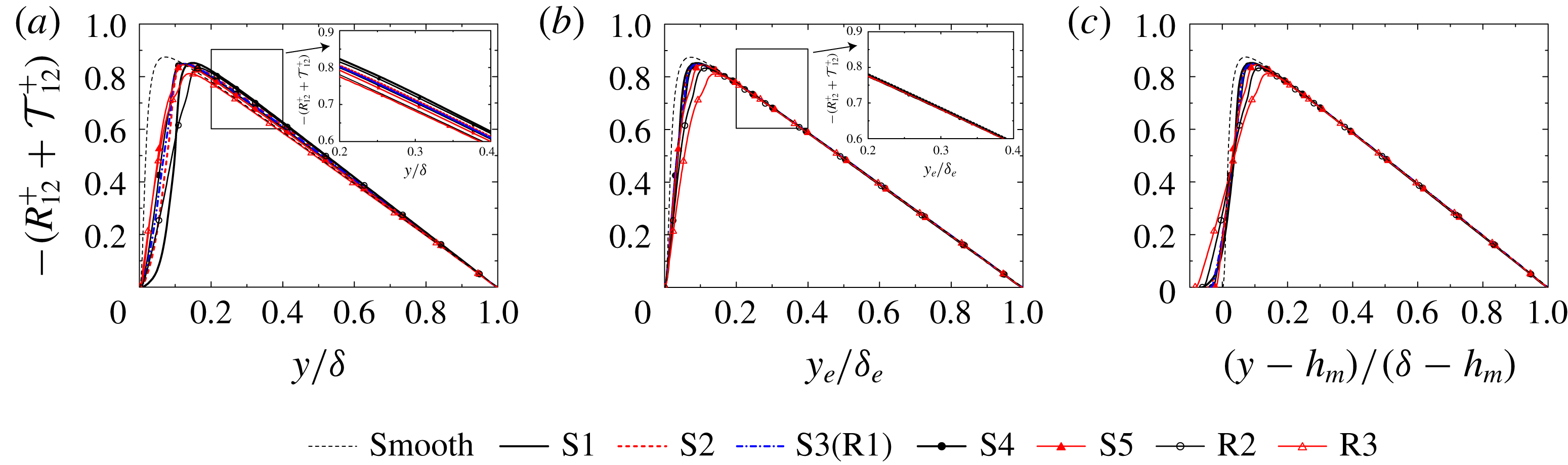
Sum of the plane-averaged Reynolds shear stress and the plane-dispersive shear stress profiles with different scalings: profiles with (a)
 $y/\unicode[STIX]{x1D6FF}$
, (b)
 $y_{e}/\unicode[STIX]{x1D6FF}_{e}$
and (c)
 $y^{\ast }=(y-h_{m})/(\unicode[STIX]{x1D6FF}-h_{m})$
. The dashed thin line indicates the smooth-wall result by Iwamoto, Suzuki & Kasagi (Reference Iwamoto, Suzuki and Kasagi2002).

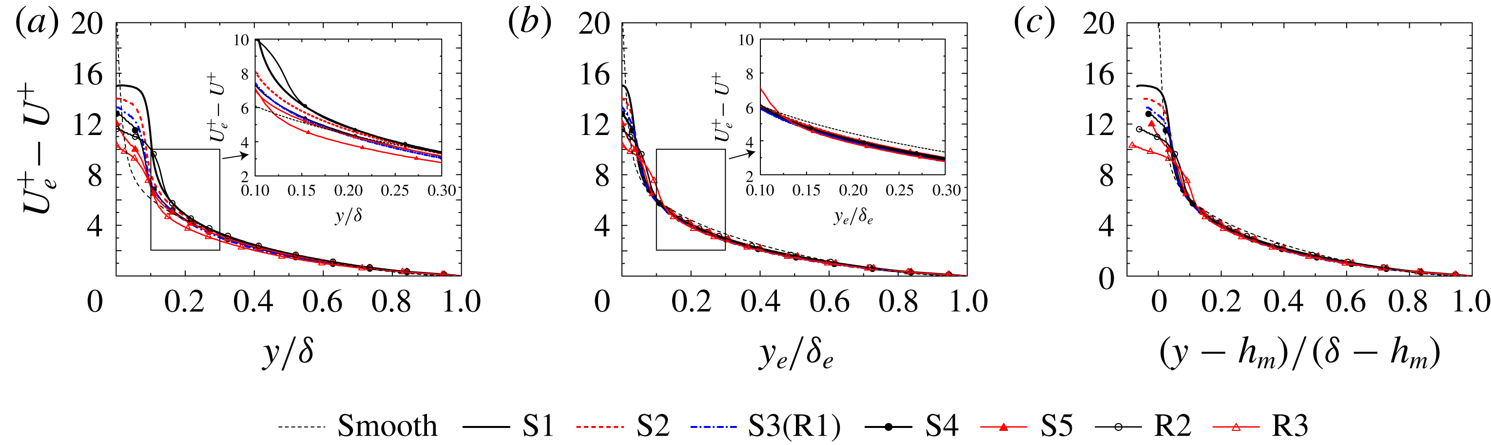
Streamwise mean velocity profiles with defect form: profiles with (a)
 $y/\unicode[STIX]{x1D6FF}$
, (b)
 $y_{e}/\unicode[STIX]{x1D6FF}_{e}$
and (c)
 $y^{\ast }=(y-h_{m})/(\unicode[STIX]{x1D6FF}-h_{m})$
. The dashed thin line indicates the smooth-wall result by Iwamoto et al. (Reference Iwamoto, Suzuki and Kasagi2002).

To demonstrate the advantage of employing the effective distance
 $y_{e}$
, profiles of the sum of the plane-averaged Reynolds shear stress
 $-R_{12}^{+}$
and the plane-dispersive shear stress
 $-{\mathcal{T}}_{12}^{+}$
for all the samples are compared between the scalings of
 $y/\unicode[STIX]{x1D6FF}$
,
 $y_{e}/\unicode[STIX]{x1D6FF}_{e}$
and
 $y^{\ast }=(y-h_{m})/(\unicode[STIX]{x1D6FF}-h_{m})$
in figure 3. For comparison, DNS results in smooth-wall turbulent channel flow at friction Reynolds number of 650 (Iwamoto et al.
Reference Iwamoto, Suzuki and Kasagi2002) are also plotted. Also, figure 4 depicts profiles of
 $U^{+}$
by defect form with reference to
 $U_{e}^{+}$
. Here,
 $U^{+}=\langle \overline{u}\rangle ^{f}$
and
 $U_{e}^{+}$
denote
 $U^{+}$
at the top slip boundary at
 $y=\unicode[STIX]{x1D6FF}$
. It is clear that the profiles of
 $-(R_{12}^{+}+{\mathcal{T}}_{12}^{+})$
as a function of
 $y_{e}/\unicode[STIX]{x1D6FF}_{e}>0.15$
and
 $y^{\ast }>0.15$
in figures 3(b) and 3(c) collapse very well, whereas the profiles as a function of
 $y/\unicode[STIX]{x1D6FF}$
in figure 3(a) do not. Jiménez (Reference Jiménez2004) pointed out that when the roughness height
 $h$
occupied a relatively large fraction of the boundary layer thickness,
 $\unicode[STIX]{x1D6FF}/h<40$
, turbulence in the whole region was modified by the roughness and then the similarity of the profiles outside the roughness sublayer was not preserved. However, almost perfect similarity can be found in the mean velocity defect with the scaling of
 $y_{e}/\unicode[STIX]{x1D6FF}_{e}$
as shown in figure 4(b) in the region of
 $y_{e}/\unicode[STIX]{x1D6FF}_{e}>0.15$
, which substantiates that the outer layer similarity may be maintained in the present rough surfaces with relatively high roughness height,
 $\unicode[STIX]{x1D6FF}/h_{m}=13{-}45$
. The observation of the similarity for the rough surfaces whose roughness height is a significant fraction of the boundary layer thickness is in accordance with the observations by another experimental study (Flack, Schultz & Connelly Reference Flack, Schultz and Connelly2007) and DNS studies (Chan et al.
Reference Chan, MacDonald, Chung, Hutchins and Ooi2015; Forooghi et al.
Reference Forooghi, Stroh, Schlatter and Frohnapfel2018a
). Moreover, the onset of the region
 $y_{e}/\unicode[STIX]{x1D6FF}_{e}=0.15$
where the similarity of the streamwise mean velocity can be clearly seen corresponds to
 $y_{e}/h_{m}=2{-}7$
. This supports the previous finding that similarity outside a roughness sublayer extends
 $5h$
from the wall (Raupach, Antonia & Rajagopalan Reference Raupach, Antonia and Rajagopalan1991). The fact that good collapse can be observed outside the roughness sublayer implies that
 $h_{m}$
can also be regarded as the displacement thickness, which is usually computed to fit the mean velocity profile to the log-law profile. Although good collapse outside the roughness sublayer can be confirmed with both scalings of
 $y_{e}$
and
 $y^{\ast }$
, a difference is obvious near the origin of the rough walls
 $y_{e}\simeq 0$
and
 $y^{\ast }\simeq 0$
. As mentioned above, as the origin of the effective distance is located at a position where there is no fluid phase,
 $\unicode[STIX]{x1D711}=0$
, the fluid velocity always goes to zero at
 $y_{e}=0$
. In contrast to that of
 $y_{e}$
, the scaling of
 $y^{\ast }$
assumes the origin to be
 $y=h_{m}$
, resulting in non-zero velocity at the origin. It is noted that the perfect collapse can be confirmed among the rough-wall results in figure 4(b,c) while the profile for a smooth wall does not perfectly agree with the rough-wall results. This discrepancy is considered to be due to the difference in the flow configurations. The present DNS is performed in the open-channel flow system while the smooth-wall result is obtained in the channel flow simulation, which may cause the difference in the mean velocity profile in the core region.
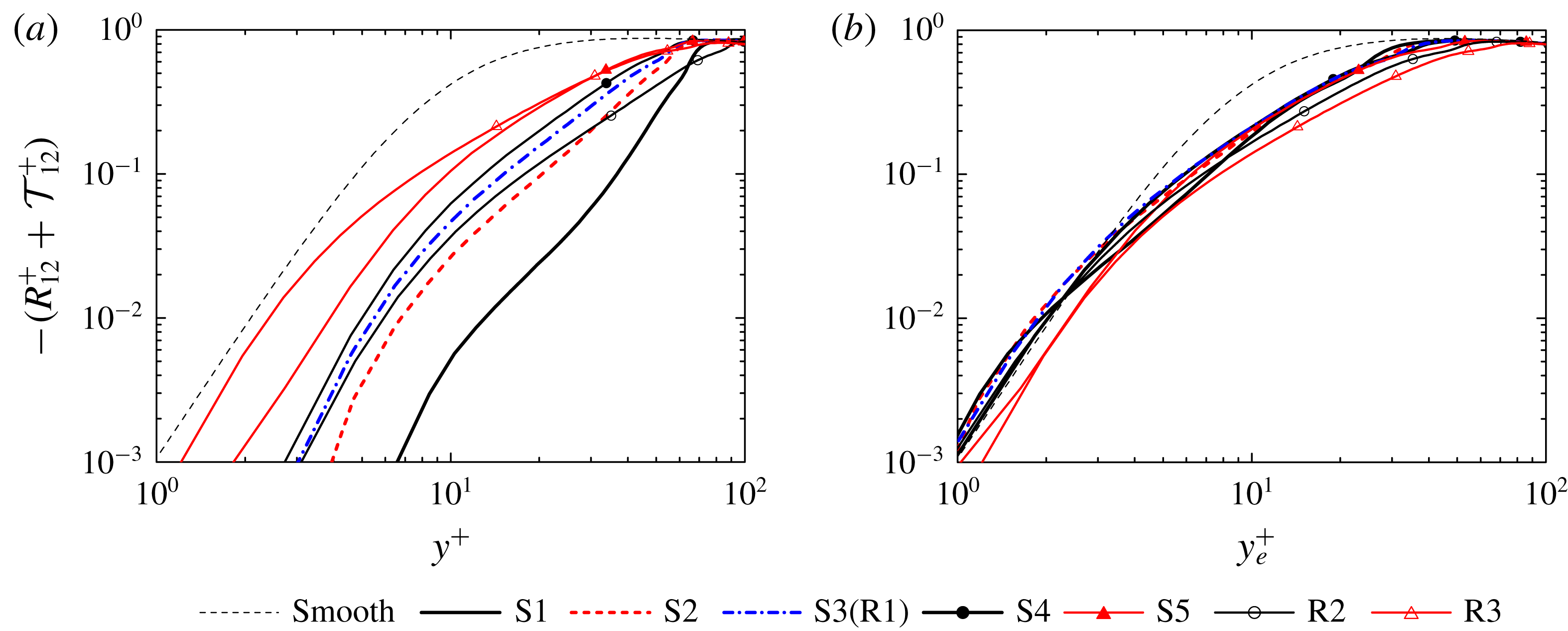
To discuss the profiles in the immediate vicinity of the origin, figure 5 compares profiles of
 $-(R_{12}^{+}+{\mathcal{T}}_{12}^{+})$
between the different scalings of
 $y^{+}$
and
 $y_{e}^{+}$
together with the smooth-wall result. The limiting behaviour of the total shear stress towards the origin with the scaling of
 $y^{+}$
is not consistent, whereas a consistent trend can be found in the profiles with
 $y_{e}^{+}$
despite the fact that the characteristics of the rough-surface geometry are very different. This suggests that the introduction of the effective distance
 $y_{e}$
enables us to compare statistics from different rough surfaces, not only outside the roughness sublayer but also in the immediate vicinity of the origin. This observation also suggests that the use of the effective distance is promising for modelling turbulence near rough surfaces. Noticeably, although the total shear stress for the rough wall is rapidly damped compared with the smooth-wall result in the region of
 $y_{e}^{+}\simeq 10$
, the limiting behaviour of the total shear stress towards the bottom wall (
 $1<y_{e}^{+}<5$
) is found to be consistent, albeit there exists the wall roughness. This observation suggests the overwhelming advantage of employing the effective distance for modelling turbulence in the vicinity of a rough wall.
Sum of the plane-averaged Reynolds shear stress and the plane-dispersive shear stress profiles in the vicinity of the origin: profiles with (a)
 $y^{+}$
and (b)
 $y_{e}^{+}$
.

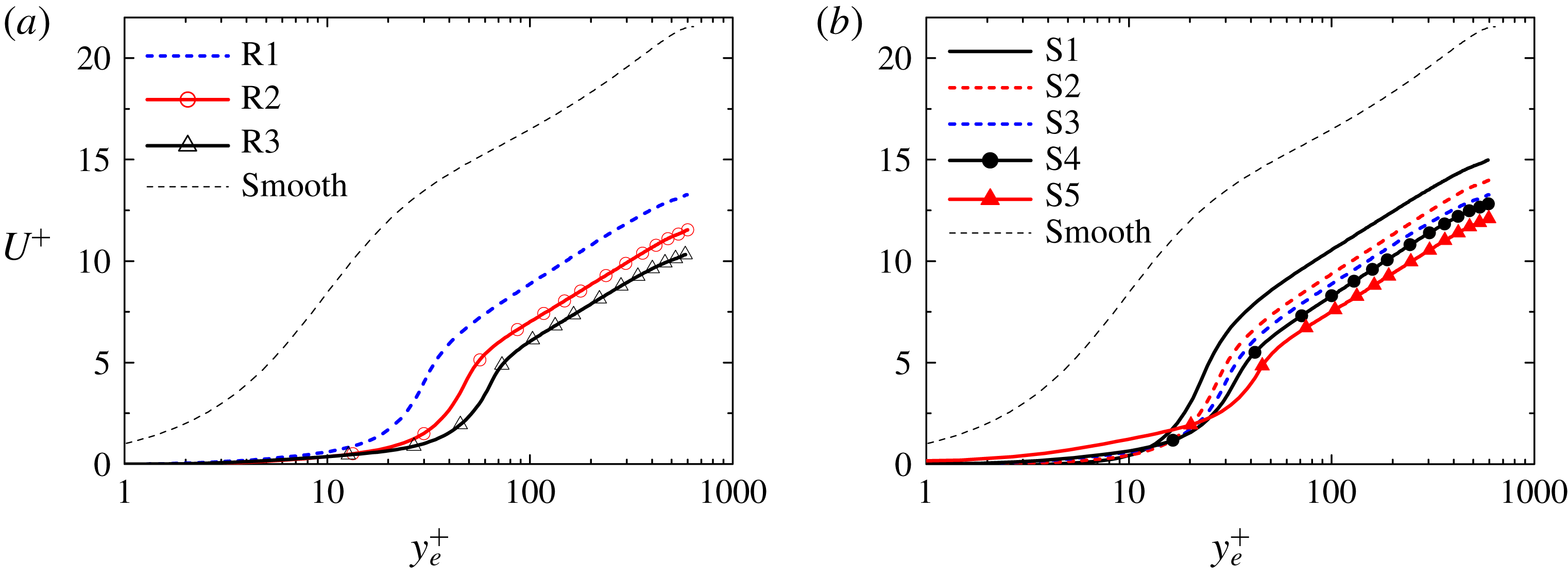
Plane-averaged streamwise mean velocity profiles with semi-logarithmic wall-scaling
 $y_{e}^{+}$
: (a) cases R1–R3 and (b) cases S1–S5. The dashed thin line indicates the smooth-wall result by Iwamoto et al. (Reference Iwamoto, Suzuki and Kasagi2002).

5.2 Mean velocity
Figure 6 presents the
 $x$
–
 $z$
plane-averaged streamwise mean velocity
 $U^{+}=\langle \overline{u}\rangle ^{f+}$
with the logarithmic scaling of the effective wall-normal distance
 $y_{e}^{+}$
together with the smooth-wall results. The profiles for the rough surfaces are significantly lower than the smooth-wall result, while the profiles seem to maintain the logarithmic profile away from the rough walls of
 $y_{e}^{+}>100$
. The mean velocity profile near the channel centre at
 $y=\unicode[STIX]{x1D6FF}$
for the smooth-wall case, however, exhibits a different trend from that observed in the rough-wall results, which is primarily due to the use of the slip boundary condition to the channel centre instead of simulating the channel flow. The downward shift of the streamwise mean velocity increases with
 $h_{rms}^{+}$
or
 $Sk$
. This indicates that rough-wall skin friction increases with increasing
 $h_{rms}^{+}$
or
 $Sk$
. The values of the downward shifts of
 $U^{+}$
referred to as roughness function
 $\unicode[STIX]{x0394}U^{+}$
are calculated by comparing
 $U^{+}$
at
 $y_{e}^{+}\simeq 100$
(
 $y_{e}/\unicode[STIX]{x1D6FF}_{e}\simeq 0.167$
) with the standard log law. Note that since the streamwise mean velocity defects in the region of
 $y_{e}/\unicode[STIX]{x1D6FF}_{e}>0.15$
are perfectly overlapped, as discussed in figure 4, the arbitrary choice of
 $y_{e}^{+}\sim 100$
does not affect the computed roughness function. (The procedure for obtaining
 $\unicode[STIX]{x0394}U^{+}$
is the same as that used by Forooghi et al. (Reference Forooghi, Stroh, Magagnato, Jakirlić and Frohnapfel2017).) The equivalent roughness
 $k_{s}^{+}$
can be uniquely determined based on the relation between
 $\unicode[STIX]{x0394}U^{+}$
and
 $k_{s}^{+}$
in the fully rough regime (Flack & Schultz Reference Flack and Schultz2010):
 $$\begin{eqnarray}B-\unicode[STIX]{x0394}U^{+}+\frac{1}{\unicode[STIX]{x1D705}}\text{ln}(k_{s}^{+})=8.5.\end{eqnarray}$$
Here,
 $\unicode[STIX]{x1D705}$
and
 $B$
respectively stand for von Kármán constant and log-law intercept for a smooth wall, and the values of
 $\unicode[STIX]{x1D705}=0.4$
and
 $B=5.0$
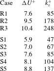
are chosen in the present study. The computed roughness functions
 $\unicode[STIX]{x0394}U^{+}$
and
 $k_{s}^{+}$
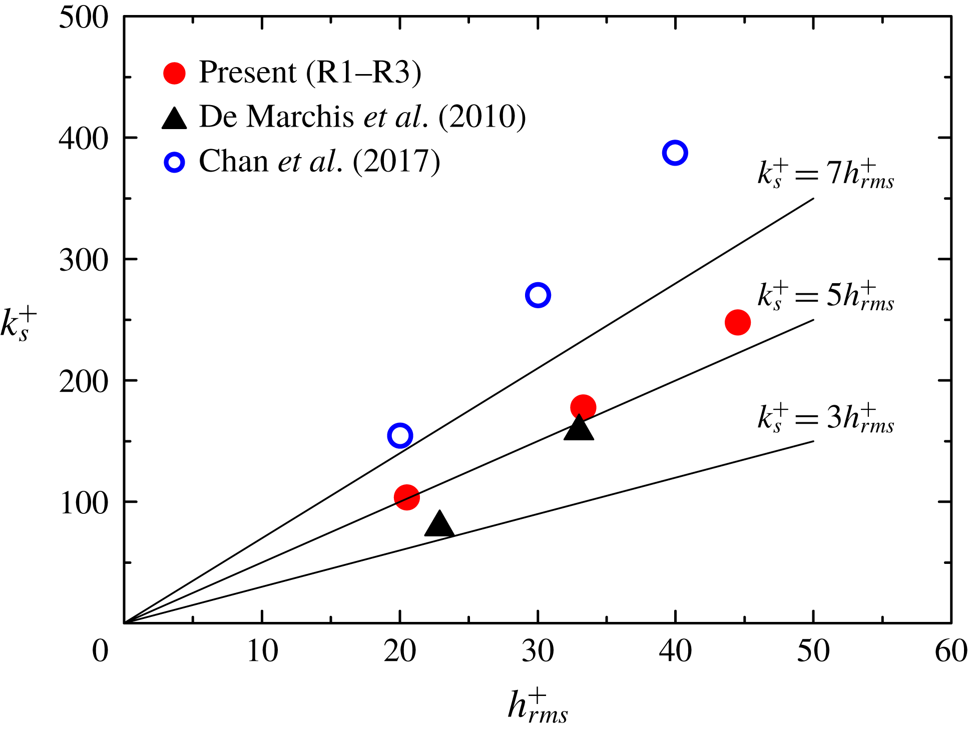
are listed in table 5. The roughness function ranges from
 $5.9$
to
 $10.4$
, and the corresponding inner-scaled equivalent roughness ranges from
 $47$
to
 $248$
. The lowest value of
 $k_{s}^{+}=47$
in case S1 roughly corresponds to the onset of the fully rough regime according to an experimental report on turbulent boundary layers over a packed sphere bed (Ligrani & Moffat Reference Ligrani and Moffat1986) in which the transitionally rough regime spanned
 $15<k_{s}^{+}<50$
. Hence, the present simulations are all expected to be in the fully rough regime. It is confirmed from table 5 that
 $k_{s}^{+}$
increases with increasing
 $h_{rms}^{+}$
or
 $Sk$
. Although the increases in
 $h_{rms}^{+}$
and
 $Sk$
both give rise in
 $k_{s}^{+}$
, the effects of the
 $h_{rms}^{+}$
and
 $Sk$
on
 $U^{+}$
profiles near the rough surface
 $y_{e}^{+}<50$
are very different. In figure 6(a), as
 $h_{rms}^{+}$
increases, the blockage effect on the
 $U^{+}$
profiles near the rough surface
 $y_{e}^{+}<50$
is more significant. In contrast, figure 6(b) confirms that the blockage effect is relaxed in the positively skewed rough wall of case S5, resulting in an increase in
 $U^{+}$
in the vicinity of the rough wall
 $y_{e}^{+}<20$
. These observations suggest that, although the increases in
 $h_{rms}^{+}$
and
 $Sk$
have the same effects on
 $\unicode[STIX]{x0394}U^{+}$
, the driving mechanism differs.
Roughness function
 $\unicode[STIX]{x0394}U^{+}$
and equivalent roughness
 $k_{s}^{+}$
.

5.3 Reynolds stress and dispersive covariance
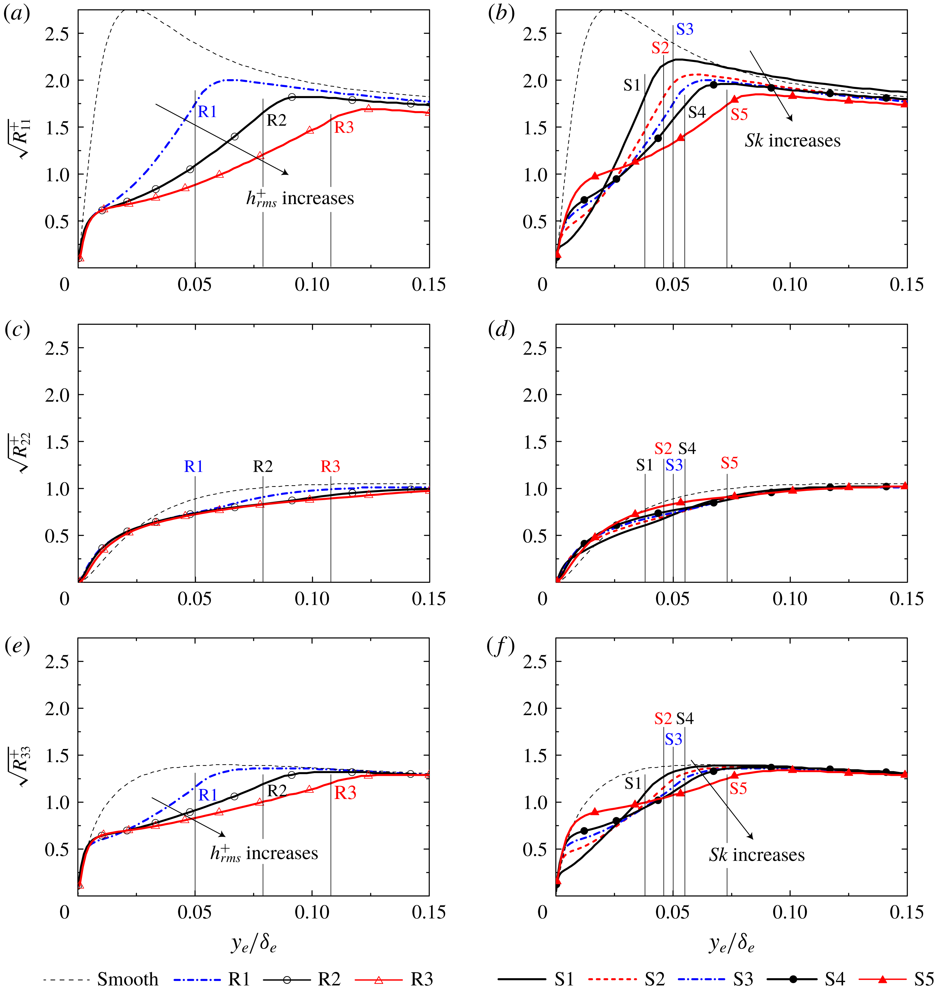
Profiles of the
 $x$
–
 $z$
plane-averaged Reynolds normal stresses
 $R_{ij}^{+}$
, which appear in the double-averaged momentum equation (5.5), are shown in figure 7. The location of the roughness peak is also indicated in the figure. In figure 7(a,c,e), as
 $h_{rms}^{+}$
increases, the Reynolds stresses are damped below the roughness peak. Reduction in the streamwise and spanwise components is pronounced in figures 7(a) and 7(e) whereas
 $R_{22}^{+}$
in figure 7(c) is insensitive to the change in the rough-surface geometry, indicating that turbulence tends to approach an isotropic state with increasing
 $h_{rms}^{+}$
. These trends are consistent with other experimental and DNS observations (Ligrani & Moffat Reference Ligrani and Moffat1986; Krogstad et al.
Reference Krogstad, Andersson, Bakken and Ashrafian2005; Flack et al.
Reference Flack, Schultz and Connelly2007; Kuwata & Suga Reference Kuwata and Suga2016b
,Reference Kuwata and Suga
c
; Forooghi et al.
Reference Forooghi, Stroh, Schlatter and Frohnapfel2018a
). In figure 7(a,c,e),
 $R_{11}^{+}$
and
 $R_{33}^{+}$
take the maximum peak just above the roughness peak, and then they are damped below the roughness peak. The significance of the damping effect depends on
 $h_{rms}^{+}$
, but the limiting behaviour of
 $R_{ij}^{+}$
towards the bottom wall is found to be similar. In figure 7(b,d,f), as
 $Sk$
increases, damping of
 $R_{11}^{+}$
and
 $R_{33}^{+}$
just below the roughness peak is more significant whereas the modification of
 $R_{22}^{+}$
is marginal, which is the same trend as in cases
 $\text{R}1{-}\text{R}3$
. However, in contrast to cases
 $\text{R}1{-}\text{R}3$
, the trends of
 $R_{11}^{+}$
and
 $R_{33}^{+}$
in the vicinity of the bottom wall
 $y_{e}/\unicode[STIX]{x1D6FF}_{e}<0.025$
are different. As
 $Sk$
increases,
 $R_{11}^{+}$
and
 $R_{33}^{+}$
gain strength in the vicinity of the bottom wall. This is because the number of hemispheres decreases with increasing
 $Sk$
, as seen in figure 1, and the blockage effect is consequently relaxed. Another important observation in the figure is that, although the behaviour of the Reynolds normal stresses near the rough surfaces of
 $y_{e}/\unicode[STIX]{x1D6FF}_{e}<0.1$
strongly depends on the roughness geometry, almost perfect collapse with the smooth-wall result can be found in
 $R_{22}^{+}$
and
 $R_{33}^{+}$
at
 $y_{e}/\unicode[STIX]{x1D6FF}_{e}=0.15$
; however, a slight discrepancy can still be found in
 $R_{11}^{+}$
at the same location.
Plane-averaged Reynolds normal stress profiles: (a) streamwise component in cases R1–R3, (b) streamwise component in cases S1–S5, (c) wall-normal component in cases R1–R3, (d) wall-normal component in cases S1–S5, (e) spanwise component in cases R1–R3, and (f) spanwise component in cases S1–S5. The location of the roughness peak is also indicated as the thin lines. The dashed thin line indicates the smooth-wall result by Iwamoto et al. (Reference Iwamoto, Suzuki and Kasagi2002).

Unlike in flows over a smooth wall, mean velocity becomes spatially inhomogeneous near rough surfaces owing to the presence of roughness elements. Hence, mean velocity dispersion defined as
 $\tilde{\overline{u}}(x,y,z)=\overline{u}(x,y,z)-\langle \overline{u}\rangle ^{f}(y)$
exists, and the plane-dispersive covariance,
 ${\mathcal{T}}_{ij}=\langle \tilde{\overline{u}}_{i}\tilde{\overline{u}}_{j}\rangle$
, accordingly arises in the double-averaged momentum equation as well as
 $R_{ij}$
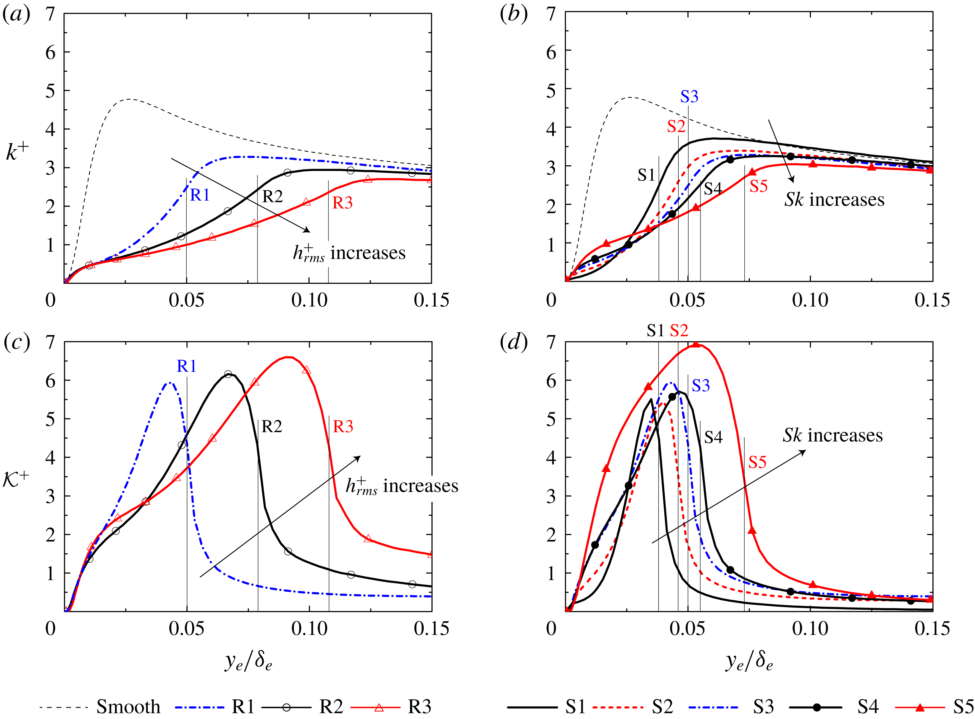
in (5.5). To compare the intensities of the mean velocity dispersion and the velocity fluctuation, the plane-dispersive kinetic energy,
 ${\mathcal{K}}^{+}={\mathcal{T}}_{kk}^{+}/2$
, and the turbulent kinetic energy,
 $k^{+}=R_{kk}^{+}/2$
, are compared in figure 8. For comparison, the turbulent kinetic energy profile for the smooth-wall case is also plotted. The figure confirms that
 ${\mathcal{K}}^{+}$
in figure 8(c,d) has a maximum below the roughness peak and it steeply decreases as it separates from the wall while
 $k^{+}$
in figure 8(a,b) has a maximum above the roughness peak. The maximum peak value of
 ${\mathcal{K}}^{+}$
is found to be far larger than that of
 $k^{+}$
in all cases, indicating that the magnitude of the mean velocity dispersion overwhelms the velocity fluctuation below the roughness peak. Although
 ${\mathcal{K}}^{+}$
steeply decreases outside the rough surfaces, it still has a meaningful value even away from the rough wall at
 $y_{e}/\unicode[STIX]{x1D6FF}_{e}=0.15$
. This implies that a spatial inhomogeneity of the mean velocity exists far away from the rough wall. The maximum peak of
 ${\mathcal{K}}^{+}$
slightly increases as
 $h_{rms}^{+}$
increases in figure 8(c), whereas the consistent trend between the maximum peak of
 ${\mathcal{K}}^{+}$
and
 $Sk$
cannot be confirmed in figure 8(d). The pronounced peak of
 ${\mathcal{K}}^{+}$
can be seen in the positively skewed rough-surface case S5, which may be due to an increase in the streamwise mean velocity in the vicinity of the rough surface in figure 6.
Plane-averaged turbulent kinetic energy and plane-dispersive kinetic energy profiles: (a) turbulent kinetic energy in cases R1–R3, (b) turbulent kinetic energy in cases S1–S5, (c) plane-dispersive kinetic energy in cases R1–R3, and (d) plane-dispersive kinetic energy in cases S1–S5. The location of the roughness peak is also indicated as the thin lines. The dashed thin line indicates the smooth-wall result by Iwamoto et al. (Reference Iwamoto, Suzuki and Kasagi2002).

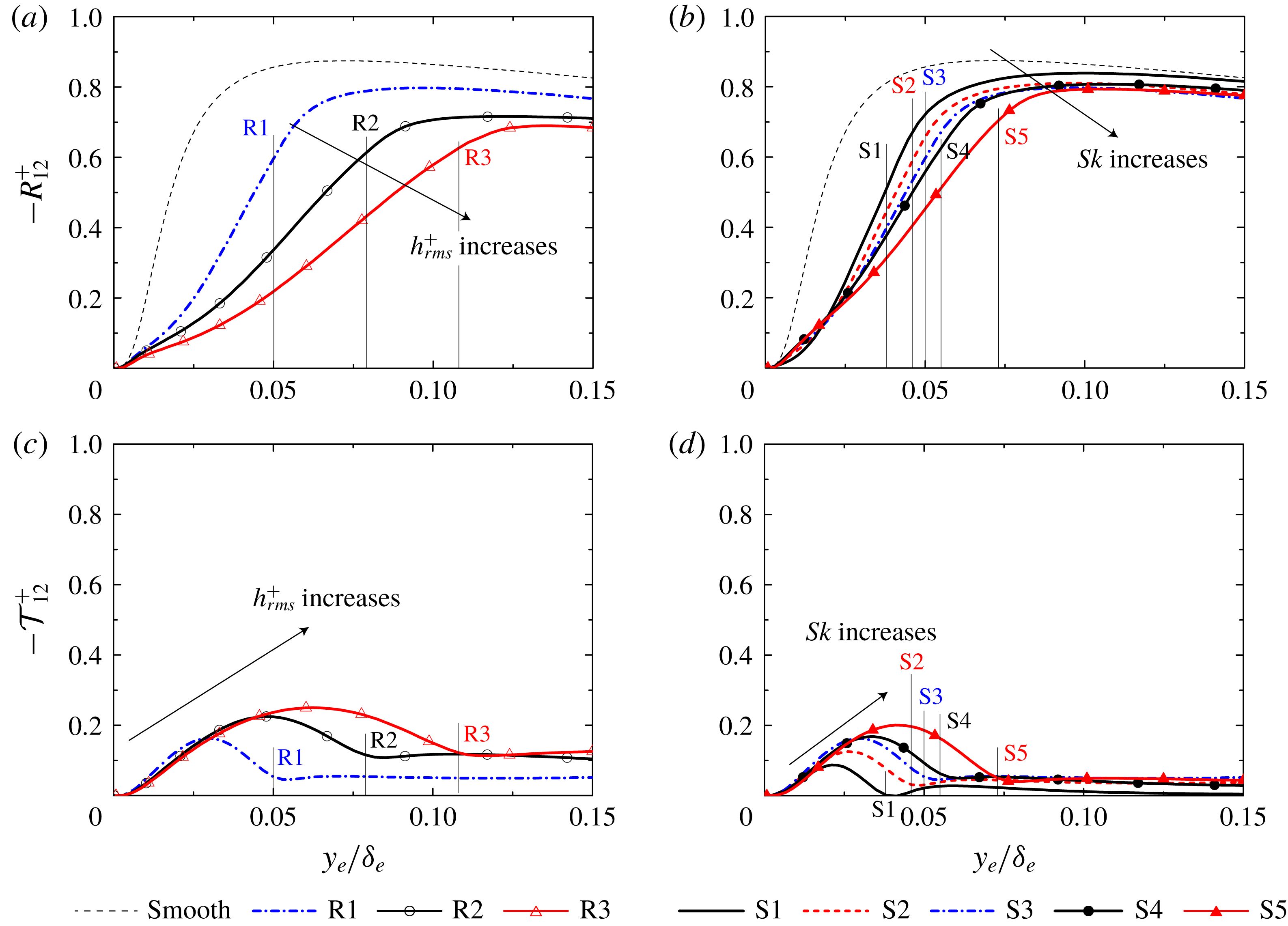
To investigate the influence of the mean velocity dispersion on the momentum transfer, figure 9 shows the contributions by the plane-averaged Reynolds shear stress
 $-R_{12}^{+}$
and the plane-dispersive covariance
 $-{\mathcal{T}}_{12}^{+}$
in the double-averaged momentum equation (5.5). The plane-dispersive covariance
 $-{\mathcal{T}}_{12}^{+}$
in figure 9(c,d) takes the maximum peak just above the roughness peak, which is similar to the trend for the plane-dispersive kinetic energy
 ${\mathcal{K}}^{+}$
in figure 8. However, the maximum peak value of
 $-{\mathcal{T}}_{12}^{+}$
is found to be far smaller than that of
 $-R_{12}^{+}$
despite the fact that the peak value of
 ${\mathcal{K}}^{+}$
overwhelms
 $k^{+}$
in figure 8. The same observation was reported in DNS studies (Busse et al.
Reference Busse, Lützner and Sandham2015; Kuwata & Kawaguchi Reference Kuwata and Kawaguchi2018). Busse et al. (Reference Busse, Lützner and Sandham2015) reported that the wall-normal velocity dispersion was approximately one order smaller than the streamwise velocity dispersion, and the plane-dispersive shear stress accordingly showed a smaller value compared with the Reynolds shear stress. In figure 9(a,c), the plane-dispersive shear stress in cases R2 and R3 has an appreciable value away from the rough surface of
 $y_{e}/\unicode[STIX]{x1D6FF}_{e}=0.15$
, whereas
 $-R_{12}^{+}$
in cases R2 and R3 shows a lower value in that region compared with its value in the smooth-wall case. However, it should be recalled that the sum of the two shear stresses,
 $-(R_{12}^{+}+{\mathcal{T}}_{12}^{+})$
, collapses irrespective of the rough geometry as seen in figure 3. The collapse of
 $-(R_{12}^{+}+{\mathcal{T}}_{12}^{+})$
indicates the collapse of the viscous shear stress, which results in the collapse of the streamwise mean velocity defect. Therefore, it can be said that the spatial inhomogeneity of the mean velocity distribution does not alter the plane-averaged streamwise mean velocity profile but alters the plane-averaged Reynolds shear stress profile.
Plane-averaged shear stress profiles: (a) plane-averaged Reynolds shear stress in cases R1–R3, (b) plane-averaged Reynolds shear stress in cases S1–S5, (c) plane-dispersive shear stress in cases R1–R3, and (d) plane-dispersive shear stress in cases S1–S5. The location of the roughness peak is also indicated as the thin lines. The dashed thin line indicates the smooth-wall result by Iwamoto et al. (Reference Iwamoto, Suzuki and Kasagi2002).

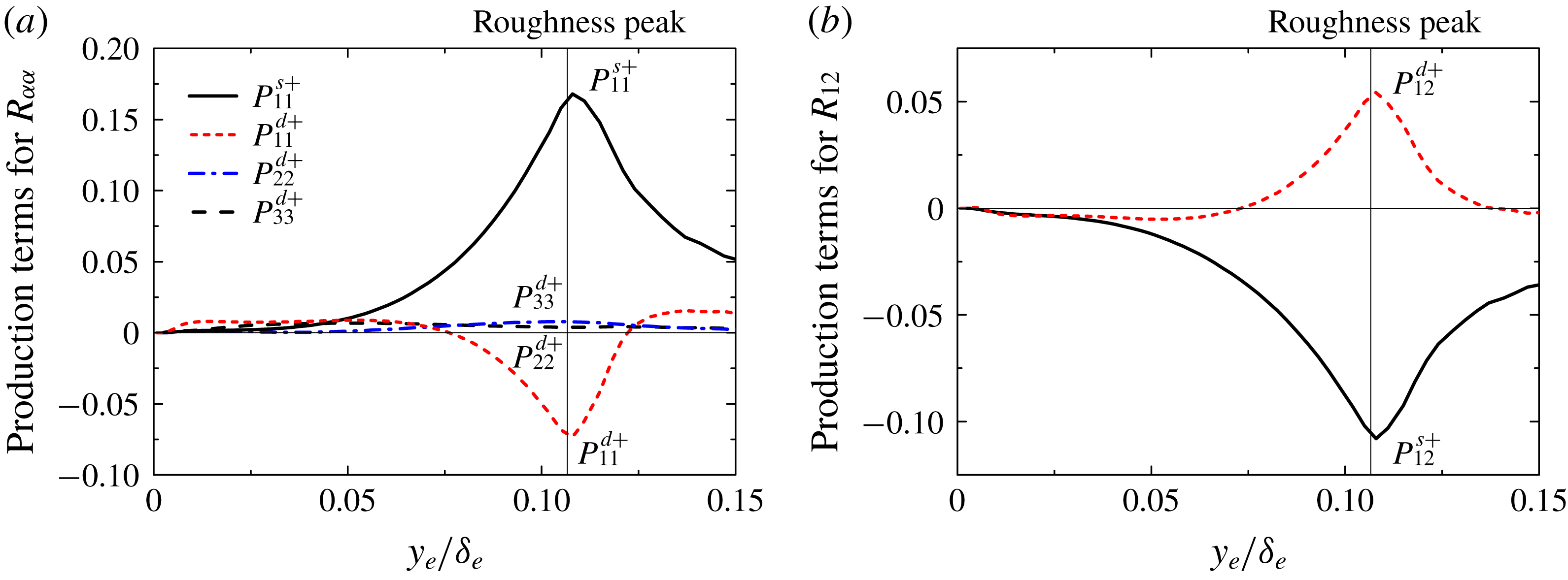
Turbulence production terms in case R3: (a) production terms for the plane-averaged Reynolds normal stresses and (b) production terms for the plane-averaged Reynolds shear stress.

For a better understanding of the influence of the mean velocity dispersion on the Reynolds stress, production terms for
 $R_{ij}^{+}$
are discussed. In the double-averaged system, two production terms, namely the mean shear production
 $P_{ij}^{s}$
and the mean dispersion-related production
 $P_{ij}^{d}$
,
 $$\begin{eqnarray}\displaystyle P_{ij}^{s} & = & \displaystyle -R_{ik}\frac{\unicode[STIX]{x2202}\langle \overline{u_{j}}\rangle ^{f}}{\unicode[STIX]{x2202}x_{k}}-R_{jk}\frac{\unicode[STIX]{x2202}\langle \overline{u_{i}}\rangle ^{f}}{\unicode[STIX]{x2202}x_{k}},\end{eqnarray}$$
 $$\begin{eqnarray}\displaystyle P_{ij}^{d} & = & \displaystyle -\unicode[STIX]{x1D711}\left\langle \left(\overline{\tilde{u} _{j}^{\prime }\tilde{u} _{k}^{\prime }}+\overline{\langle u_{k}^{\prime }\rangle ^{f}\tilde{u} _{j}^{\prime }}+\overline{\tilde{u} _{k}^{\prime }\langle u_{j}^{\prime }\rangle ^{f}}\right)\frac{\unicode[STIX]{x2202}\tilde{\overline{u}}_{i}}{\unicode[STIX]{x2202}x_{k}}\right\rangle ^{f}\nonumber\\ \displaystyle & & \displaystyle -\,\unicode[STIX]{x1D711}\left\langle \left(\overline{\tilde{u} _{i}^{\prime }\tilde{u} _{k}^{\prime }}+\overline{\langle u_{k}^{\prime }\rangle ^{f}\tilde{u} _{i}^{\prime }}+\overline{\tilde{u} _{k}^{\prime }\langle u_{i}^{\prime }\rangle ^{f}}\right)\frac{\unicode[STIX]{x2202}\tilde{\overline{u}}_{j}}{\unicode[STIX]{x2202}x_{k}}\right\rangle ^{f},\end{eqnarray}$$
can be defined (Kuwata & Suga Reference Kuwata and Suga2016c
). The production term of
 $P_{ij}^{s}$
is the turbulence generation due to the mean shear of the plane-averaged mean velocity, and the components of
 $P_{11}^{s}$
and
 $P_{22}^{s}$
remain in the present flow system because
 $\unicode[STIX]{x2202}\langle \overline{u}\rangle ^{f}/\unicode[STIX]{x2202}y$
exists. On the other hand, the production of
 $P_{ij}^{d}$
termed as the mean dispersion-related production is the production term due to the dispersive mean velocity gradients, and all components
 $P_{11}^{d},P_{22}^{d},P_{33}^{d}$
and
 $P_{12}^{d}$
have the possibility to appear near the rough surfaces. It should be mentioned that
 $P_{ij}^{d}$
also appears in the transport equation of
 ${\mathcal{T}}_{ij}$
with an opposite sign (Kuwata & Suga Reference Kuwata and Suga2016c
), and thus
 $P_{ij}^{d}$
is interpreted as an energy transfer term between
 ${\mathcal{T}}_{ij}$
and
 $R_{ij}$
. The contributions of those productions (
 $P_{ij}^{s}$
and
 $P_{ij}^{d}$
) normalized by
 $u_{\unicode[STIX]{x1D70F}}$
and
 $\unicode[STIX]{x1D708}$
in case R3, in which the mean velocity dispersion intensity is the most significant as shown in figure 8, are compared in figure 10. The productions due to the mean shear
 $P_{11}^{s}$
and
 $P_{12}^{s}$
are found to be the dominant contributors to the generation of
 $R_{11}$
and
 $R_{22}$
. In terms of the production terms for
 $R_{11}$
and
 $R_{22}$
, the sign of the mean dispersion-related production
 $P_{ij}^{d}$
is the opposite sign of
 $P_{ij}^{s}$
near the roughness peak
 $0.075<y_{e}/\unicode[STIX]{x1D6FF}_{e}<0.13$
. This indicates that
 $P_{ij}^{d}$
acts as a sink term for
 $R_{ij}$
near the roughness peak. The magnitude of the peak values of
 $P_{11}^{d+}$
and
 $P_{12}^{d+}$
near the roughness peak reach 44 % of
 $P_{11}^{s+}$
and 50 % of
 $P_{12}^{s+}$
, respectively. Although the terms
 $P_{11}^{d}$
and
 $P_{12}^{d}$
substantially reduce
 $R_{11}$
and
 $R_{22}$
near the roughness peak region of
 $0.075<y_{e}/\unicode[STIX]{x1D6FF}_{e}<0.13$
, it is observed that they work as a source in the other region. In contrast to
 $P_{11}^{d}$
and
 $P_{12}^{d}$
, the other components
 $P_{22}^{d}$
and
 $P_{33}^{d}$
do not work as sink terms, but their contributions are found to be small. The significance of
 $P_{11}^{d}$
and
 $P_{12}^{d}$
partly explains the noticeable reduction in the streamwise Reynolds stress and the Reynolds shear stress near the roughness peak as observed in figure 7. Furthermore, this also explains the discrepancies in
 $R_{11}^{+}$
and
 $R_{12}^{+}$
even away from the rough wall of
 $y_{e}/\unicode[STIX]{x1D6FF}_{e}=0.15$
in figures 7 and 9 because the significance of
 $P_{11}^{d}$
and
 $P_{12}^{d}$
, which are generated due to the dispersive mean velocity gradients, strongly depends on the roughness topology. Additionally, considering that
 $P_{12}^{d}$
appears in the transport equation of
 ${\mathcal{T}}_{12}$
with an opposite sign, it can be said that a reduction in
 $R_{12}$
leads to the generation of
 ${\mathcal{T}}_{12}$
. This may also explain the observation that the sum of
 $-(R_{12}^{+}+{\mathcal{T}}_{12}^{+})$
collapses in all cases irrespective of the significance of
 ${\mathcal{T}}_{12}^{+}$
as shown in figures 3 and 9. However, to give a complete answer, a full budget term analysis for
 ${\mathcal{T}}_{ij}$
and
 $R_{ij}$
is essential.
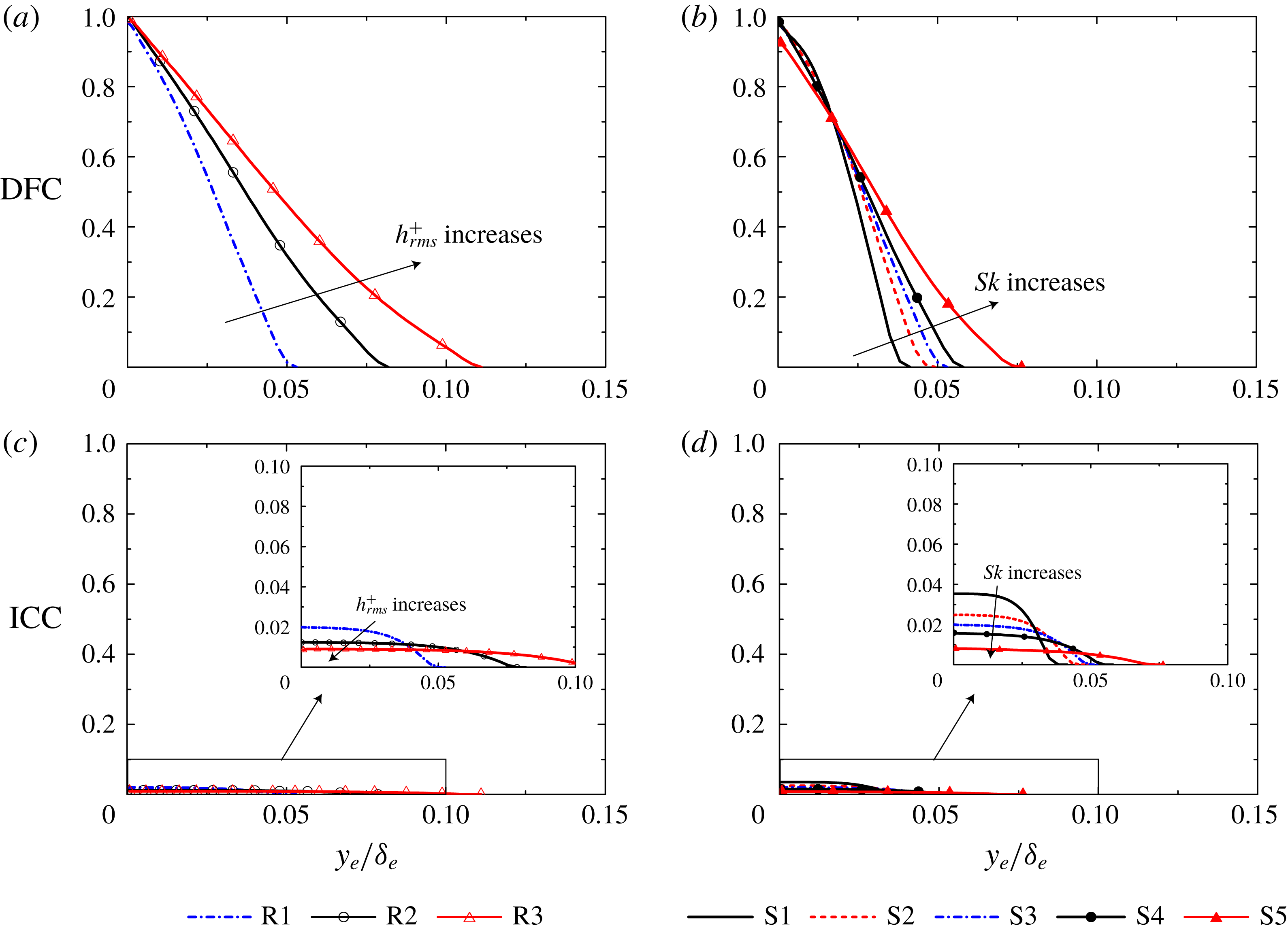
Plane-averaged drag force contribution (DFC) and the inhomogeneous correction contribution (ICC): (a) DFC in cases R1–R3, (b) DFC in cases S1–S5, (c) ICC in cases R1–R3, and (d) ICC in cases S1–S5.

5.4 Drag force and inhomogeneous correction terms
The plane-averaged Reynolds shear stress and the plane-dispersive covariance are damped on approaching the bottom wall at
 $y_{e}/\unicode[STIX]{x1D6FF}_{e}=0$
, while the inhomogeneous correction contribution (ICC) and the drag force contribution (DFC) in (5.5), defined as
 $$\begin{eqnarray}\left.\begin{array}{@{}c@{}}\displaystyle ICC=-\left(\int _{0}^{y}\unicode[STIX]{x1D711}\overline{g}_{x}^{\unicode[STIX]{x1D711}}\,\text{d}y-\int _{0}^{\unicode[STIX]{x1D6FF}}\unicode[STIX]{x1D711}\overline{g}_{x}^{\unicode[STIX]{x1D711}}\,\text{d}y\right),\\ \displaystyle DFC=-\left(\int _{0}^{y}\unicode[STIX]{x1D711}\overline{f}_{x}\,\text{d}y-\displaystyle \int _{0}^{\unicode[STIX]{x1D6FF}}\unicode[STIX]{x1D711}\overline{f}_{x}\,\text{d}y\right),\end{array}\right\}\end{eqnarray}$$
are generated below the roughness peak instead. To investigate the contribution of ICC and DFC defined in (5.16), the terms (DFC and ICC) are normalized by
 $u_{\unicode[STIX]{x1D70F}}$
(figure 11). The drag force term DFC in figure 11(a) and (b) increases towards the bottom wall of
 $y_{e}/\unicode[STIX]{x1D6FF}_{e}=0$
and it reaches almost unity because the other stress terms become negligibly small at the bottom wall. However, in case S5, as a slight viscous stress exists at the bottom wall (not shown here), DFC shows a lower value at
 $y_{e}/\unicode[STIX]{x1D6FF}_{e}=0$
compared with those in the other cases. In contrast to DFC, the contribution of ICC in figure 11(c) and (d) is negligibly smaller compared with DFC. As
 $h_{rms}^{+}$
or
 $Sk$
increases, the location of the roughness peak scaled with the effective distance moves away from the bottom wall, and then the influence of DFC and ICC extends away from the bottom wall. The term ICC at the bottom wall is found to consistently decrease with
 $Sk$
or
 $h_{rms}^{+}$
.
5.5 Skin friction coefficient
This subsection discusses the contribution of the stress terms in (5.6) to the skin friction coefficient
 $C_{f}$
defined as
 $C_{f}=\unicode[STIX]{x1D70F}_{w}/(0.5\unicode[STIX]{x1D70C}U_{b}^{2})$
. Here, the bulk mean velocity is computed with the mass flow rate
 $Q$
divided by the effective cross-sectional area
 $S_{yz}$
as
 $U_{b}=Q/S_{yz}$
. Applying further double integration over the wall-normal direction to (5.6) with normalization of
 $\unicode[STIX]{x1D6FF}$
and
 $2U_{b}$
, the FIK identity (Fukagata, Iwamoto & Kasagi Reference Fukagata, Iwamoto and Kasagi2002) for the double-averaged system can be derived as
 $$\begin{eqnarray}\displaystyle C_{f} & = & \displaystyle \underbrace{\frac{\unicode[STIX]{x1D6FF}_{e}}{\unicode[STIX]{x1D6FF}C^{\prime }}\frac{4}{Re_{b}}}_{laminar}\underbrace{+\,\frac{8}{C^{\prime }}\int _{0}^{1}\left(1-y\right)\left(-R_{12}\right)\,\text{d}y}_{turbulence}\underbrace{+\frac{8}{C^{\prime }}\int _{0}^{1}\left(1-y\right)\left(-{\mathcal{T}}_{12}\right)\,\text{d}y}_{dispersion}\nonumber\\ \displaystyle & & \displaystyle \underbrace{+\,\frac{8}{C^{\prime }}\int _{0}^{1}\left(y-\frac{1}{2}y^{2}\right)\left(\unicode[STIX]{x1D711}\overline{f}_{x}\right)\,\text{d}y}_{drag}\underbrace{+\,\frac{8}{C^{\prime }}\int _{0}^{1}\left(y-\frac{1}{2}y^{2}\right)\left(\unicode[STIX]{x1D711}\overline{g^{\unicode[STIX]{x1D711}}}_{x}\right)\,\text{d}y}_{inhomogeneous~correction},\end{eqnarray}$$
where
 $Re_{b}$
is the bulk mean Reynolds number, and constant
 $C^{\prime }$
is expressed as
 $$\begin{eqnarray}C^{\prime }=\frac{\unicode[STIX]{x1D6FF}}{\unicode[STIX]{x1D6FF}_{e}}\int _{0}^{1}\left(y-\frac{1}{2}y^{2}\right)\unicode[STIX]{x1D711}\,\text{d}y.\end{eqnarray}$$
In addition to the laminar and turbulence contributions, the dispersion, drag and inhomogeneous correction contribution terms appear as contributors to
 $C_{f}$
owing to the presence of a rough surface. (See appendix A for the detailed derivation of (5.17).) As well as the turbulence contribution, the dispersion contribution is expressed as an integration of the weighted plane-dispersive covariance
 $(1-y){\mathcal{T}}_{12}$
, which suggests that
 ${\mathcal{T}}_{12}$
near the bottom wall contributes more to the skin friction coefficient. Unlike
 $R_{12}$
and
 ${\mathcal{T}}_{12}$
, the weighting function for
 $\overline{f}_{x}$
and
 $\overline{g}_{x}^{\unicode[STIX]{x1D711}}$
,
 $(y-\frac{1}{2}y^{2})$
, increases with distance from the bottom wall, suggesting that
 $\overline{f}_{x}$
and
 $\overline{g}_{x}^{\unicode[STIX]{x1D711}}$
away from the bottom wall contribute more to the skin friction coefficient. Additionally, unlike the FIK identity for the turbulent channel or pipe flows as discussed by Fukagata et al. (Reference Fukagata, Iwamoto and Kasagi2002), the constant
 $C^{\prime }$
appears in the denominator of each contribution. Hence, all contributions are consistently affected depending on the value of
 $C^{\prime }$
. When we consider the smooth channel flow (i.e.
 $\unicode[STIX]{x1D711}=1$
for the entire region and
 $\unicode[STIX]{x1D6FF}_{e}=\unicode[STIX]{x1D6FF}$
),
 $C^{\prime }$
takes value
 $1/3$
and (5.17) consequently reduces to the FIK identity for the fully developed turbulent channel flow. For the presently tested rough surfaces, however, variation in
 $C^{\prime }$
is not significant;
 $C^{\prime }$
varies in the range from 0.34 (case S5) to 0.35 (case R3). Hence, the value of
 $C^{\prime }$
is not a key parameter that determines
 $C_{f}$
in the presently tested cases.
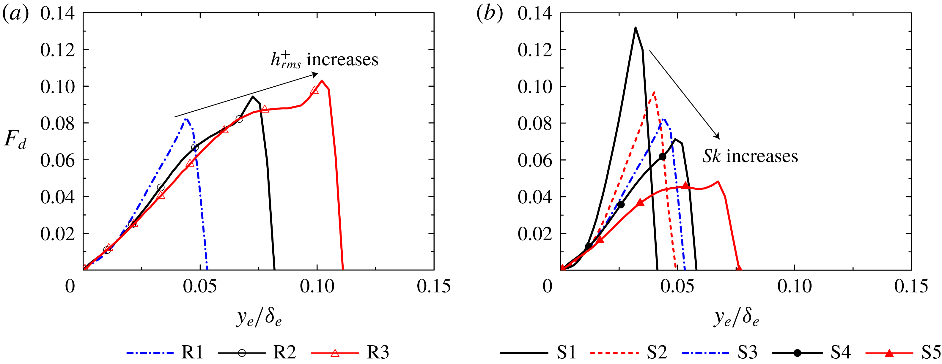
Weighted drag force term of (5.19): (a) cases R1–R3 and (b) cases S1–S5.

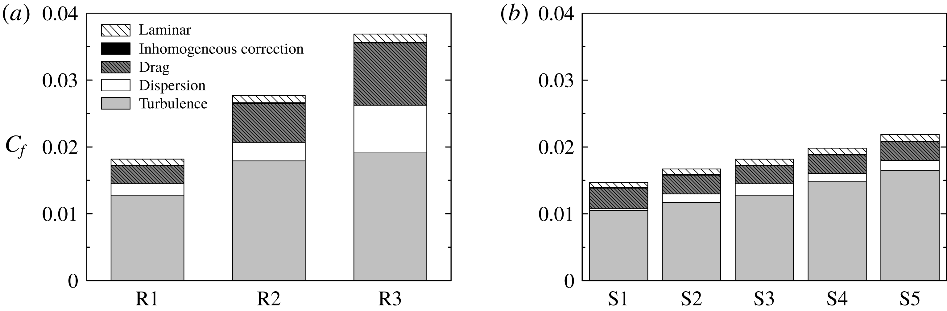
The contribution terms in (5.17) are presented in figure 13. It is revealed that the most dominant contribution to
 $C_{f}$
is turbulence, and the second contribution is the drag force in all cases. The laminar contribution is almost independent of the change in
 $h_{rms}^{+}$
or
 $Sk$
, and the inhomogeneous correction term is found to hardly contribute to an increase in
 $C_{f}$
. The dispersion contribution increases with increasing
 $h_{rms}^{+}$
in figure 13(a) and its contribution in case R3 reaches 37 % of the turbulence contribution. In contrast, as shown in figure 13(b), the dispersion contribution is far smaller compared with the turbulence contribution, and the dispersion contribution takes almost an constant value irrespective of the change in
 $Sk$
. In terms of the turbulence and drag force contribution terms, the turbulence and drag force contribution terms in figure 13(a) increase with
 $h_{rms}^{+}$
. In particular, the increase in the drag contribution is found to be prominent (the drag contribution in case R3 is
 $3.3$
times larger than that in case R1). In contrast, it is observed in figure 13(b) that an increase in
 $Sk$
dose not significantly affect an increase in the drag contribution while the turbulence contribution increases with
 $Sk$
. Hence, it is understood that the impacts of
 $h_{rms}^{+}$
and
 $Sk$
on the drag force contribution are different.
To identify the reason for these observations, figure 12 shows the integral function for the drag force contribution defined as follows:
 $$\begin{eqnarray}F_{d}(y)=\frac{8}{C^{\prime }}\left(y-\frac{1}{2}y^{2}\right)\left(\unicode[STIX]{x1D711}\overline{f}_{x}\right).\end{eqnarray}$$
Corresponding to an increase in the roughness peak height scaled with the effective distance with
 $h_{rms}^{+}$
or
 $Sk$
, the influence of
 $F_{d}$
is extended away from the bottom wall with
 $h_{rms}^{+}$
or
 $Sk$
. However, it is observed that the maximum peak of
 $F_{d}$
in figure 12(b) steeply decreases with increasing
 $Sk$
while the maximum peak of
 $F_{d}$
in figure 12(a) gradually increases with
 $h_{rms}^{+}$
. The primary reason for the decrease in the maximum peak
 $F_{d}$
with
 $Sk$
is a decrease in the surface area of the roughness element. Since the pressure and viscous drag terms are expressed as the sum of the surface integration of the viscous stress and the pressure per a certain
 $x$
–
 $z$
plane as in (5.5), the decrease in the surface area directly results in a decrease in the drag force. As
 $Sk$
increases, the number of hemispheres decreases, keeping the hemisphere diameter almost constant, which obviously decreases the surface area, as can be seen in figure 1, resulting in the decrease in
 $F_{d}$
.
Contribution terms to the skin friction coefficient in (5.17): (a) cases R1–R3 and (b) cases S1–S5.

Variation of
 $k_{s}^{+}$
with
 $h_{rms}^{+}$
; data of De Marchis et al. (Reference De Marchis, Napoli and Armenio2010) are for two-dimensional irregular wavy walls and data of Chan et al. (Reference Chan, MacDonald, Chung, Hutchins and Ooi2015) are for three-dimensional sinusoidal rough walls.

5.6 Improvement of correlation function for the equivalent roughness
This subsection concentrates on the relation between the equivalent roughness and the statistical moments, namely
 $h_{rms}^{+}$
and
 $Sk$
. However, it should be cautioned that equivalent roughness is not a physical property but a flow property, and the equivalent roughness is not necessarily guaranteed to have a relation with the roughness topological parameters. Figure 14 shows the variation in
 $k_{s}^{+}$
with
 $h_{rms}^{+}$
in case R1–R3. For comparison, we also plot data for the rough surfaces of
 $Sk\simeq 0$
and
 $ES>0.35$
in the fully rough regime, namely two-dimensional irregular wavy walls (De Marchis et al.
Reference De Marchis, Napoli and Armenio2010) and three-dimensional sinusoidal rough walls (Chan et al.
Reference Chan, MacDonald, Chung, Hutchins and Ooi2015). Furthermore, linear lines with slopes of 3.0, 5.0 and 7.0 are shown. It is observed that
 $k_{s}^{+}$
in the present data linearly increases with
 $h_{rms}^{+}$
, and the factor of the proportionality is approximately
 $5.0$
. The results in two-dimensional irregular wavy walls by De Marchis et al. (Reference De Marchis, Napoli and Armenio2010) are close to the present results of cases R1 and R2 whereas the data of Chan et al. (Reference Chan, MacDonald, Chung, Hutchins and Ooi2015) are substantially larger than the present results. The discrepancy can be partly explained by the difference in the roughness arrangement. The rough surfaces in this study and the rough surfaces of De Marchis et al. (Reference De Marchis, Napoli and Armenio2010) are irregular while the roughness corrugations of Chan et al. (Reference Chan, MacDonald, Chung, Hutchins and Ooi2015) are regularly aligned with a staggered arrangement. Forooghi et al. (Reference Forooghi, Stroh, Magagnato, Jakirlić and Frohnapfel2017) reported that the staggered arrangement of the roughness elements resulted in higher equivalent roughness compared with randomly distributed roughness elements. Another implication in terms of the discrepancy is the presence of more suitable roughness height parameters. Indeed, although the present study chooses
 $h_{rms}$
as the roughness height parameter, there are different possible choices for the roughness height parameter (e.g. mean peak height, peak-to-valley height, or roughness height amplitude). However, as the data are not sufficient to explore alternative parameters to
 $h_{rms}$
, we do not discuss it here. (See Flack & Schultz (Reference Flack and Schultz2010), Flack, Schultz & Rose (Reference Flack, Schultz and Rose2012), Forooghi et al. (Reference Forooghi, Stroh, Magagnato, Jakirlić and Frohnapfel2017) and Thakkar et al. (Reference Thakkar, Busse and Sandham2017) for detailed discussions on the peak-to-valley height, and see De Marchis et al. (Reference De Marchis, Napoli and Armenio2010) and Chan et al. (Reference Chan, MacDonald, Chung, Hutchins and Ooi2015) for the roughness height amplitude.) In terms of the relation between
 $h_{rms}$
and
 $k_{s}$
, Flack & Schultz (Reference Flack and Schultz2010) derived a correlation by fitting a large number of experimental data, including several kinds of real rough surfaces:
 $$\begin{eqnarray}k_{s}=4.43h_{rms}(1+Sk)^{1.37}.\end{eqnarray}$$
The correlation suggests that the proportionality constant becomes
 $4.43$
for
 $Sk=0$
, which is found to be close to the value obtained by the present DNS. The other reports on the relation between
 $k_{s}$
and
 $h_{rms}$
state that
 $k_{s}\sim 3h_{rms}$
for honed surfaces (Shockling, Allen & Smits Reference Shockling, Allen and Smits2006) and
 $k_{s}\sim 1.6h_{rms}$
for a commercial steel pipe (Langelandsvik et al.
Reference Langelandsvik, Kunkel and Smits2008), whose proportionality constants are significantly lower than those obtained in this study. However, it should be cautioned that those proportionality constants were not for rough surfaces of
 $Sk=0$
.
Variation
 $k_{s}/h_{rms}$
against
 $Sk$
; data of Schultz & Flack (Reference Schultz and Flack2009) are for pyramid roughness, data of Yuan & Piomelli (Reference Yuan and Piomelli2014) are for numerically generated sand grains, data of Busse et al. (Reference Busse, Thakkar and Sandham2017) are for graphite roughness and grit-blasted roughness, data of Forooghi et al. (Reference Forooghi, Stroh, Schlatter and Frohnapfel2018a
) are for randomly distributed hemispheres/cones, and data of Forooghi et al. (Reference Forooghi, Weidenlener, Magagnato, Böhm, Kubach, Koch and Frohnapfel2018b
) are for combustion chamber deposits. The dashed line indicates the correlation of (5.20) (Flack & Schultz Reference Flack and Schultz2010), and the solid line indicates the fitted curve of (5.21).

To see the influence of
 $Sk$
on
 $k_{s}^{+}$
, figure 15 shows
 $k_{s}/h_{rms}$
versus
 $Sk$
. For comparison, we also plot experimental data for pyramid roughness (Schultz & Flack Reference Schultz and Flack2009), and other DNS data for randomly distributed hemispheres/cones (Forooghi et al.
Reference Forooghi, Stroh, Schlatter and Frohnapfel2018a
), graphite roughness (Busse et al.
Reference Busse, Thakkar and Sandham2017), grit-blasted roughness (Busse et al.
Reference Busse, Thakkar and Sandham2017), numerically generated sand grains (Yuan & Piomelli Reference Yuan and Piomelli2014) and combustion chamber deposits (Forooghi et al.
Reference Forooghi, Weidenlener, Magagnato, Böhm, Kubach, Koch and Frohnapfel2018b
) with
 $ES>0.35$
. The dashed line indicates the correlation function of (5.20) by Flack & Schultz (Reference Flack and Schultz2010), and the solid line displays the best-fitted curve
 $$\begin{eqnarray}k_{s}/h_{rms}=4.0\left(1+0.17Sk\right)^{4}.\end{eqnarray}$$
Clearly, all the results suggest that
 $k_{s}^{+}$
monotonically increases with
 $Sk$
in the range
 $-1<Sk<3$
. This observation is in line with the correlation of Flack & Schultz (Reference Flack and Schultz2010) whereas it is in contrast to the findings by Flack et al. (Reference Flack, Schultz, Barros and Kim2016) that an increase in
 $Sk$
slightly reduces
 $k_{s}$
. It should be noted that the finding by Flack et al. (Reference Flack, Schultz, Barros and Kim2016) was, however, based on experimental data for grit-blasted surfaces with negative skewness, and is not the implication for a generic rough surface. The correlation function by Flack & Schultz (Reference Flack and Schultz2010) reasonably works in the range of
 $-0.5<Sk<0.5$
; however, the correlation function is found to overestimate the influence of
 $Sk$
in the rough-wall case with significantly positive/negative skewness
 $Sk<-0.5,~Sk>0.5$
. One possible reason for the discrepancy is the influence of small short-wavelength undulation. Besides the numerically generated rough surfaces in Chan et al. (Reference Chan, MacDonald, Chung, Hutchins and Ooi2015) and Forooghi et al. (Reference Forooghi, Stroh, Magagnato, Jakirlić and Frohnapfel2017) and the presently used samples, real rough surfaces usually include short- and long-wavelength undulations. Howell & Behrends (Reference Howell and Behrends2006) reported in terms of measurements on real rough surfaces that sampling interval and sampling length had significant effects on roughness statistics. The rough-surface samples used in the DNS (Busse et al.
Reference Busse, Thakkar and Sandham2017; Forooghi et al.
Reference Forooghi, Weidenlener, Magagnato, Böhm, Kubach, Koch and Frohnapfel2018b
) were filtered to remove uninfluential undulation by the low-pass filter. Additionally, it should be noted that DNS can completely reflect the scanned rough-surface geometry even though they contain some measurement uncertainty originating from insufficiency of resolution, sampling interval or sampling length. On the other hand, as the samples used in Flack & Schultz (Reference Flack and Schultz2010) were not filtered, the influence of the short-wavelength undulation or the measurement condition may emerge. Another possible reason for the underprediction of
 $k_{s}/h_{rms}$
for the rough surfaces with
 $Sk<-0.5$
by Flack & Schultz (Reference Flack and Schultz2010) is that only two samples were used in Flack & Schultz (Reference Flack and Schultz2010) which had negative skewness, and both were relatively mild (
 $Sk=-0.455,-0.19$
). The values
 $k_{s}/h_{rms}$
are inconsistent even though
 $Sk$
are the same, which is clearly seen in the results by Schultz & Flack (Reference Schultz and Flack2009) and Forooghi et al. (Reference Forooghi, Weidenlener, Magagnato, Böhm, Kubach, Koch and Frohnapfel2018b
). This points out the fact that
 $k_{s}/h_{rms}$
is not simply expressed as a function of
 $Sk$
, but other roughness parameters should be included to take account of the other roughness characteristics such as the slope or the solidity. Indeed, Forooghi et al. (Reference Forooghi, Stroh, Magagnato, Jakirlić and Frohnapfel2017) demonstrated that peak height distribution independently affected the equivalent roughness as well as the skewness and the effective slope, and Thakkar et al. (Reference Thakkar, Busse and Sandham2017) presented the significant impact of the streamwise correlation length on the equivalent roughness. Since the presently used data are limited, it is unknown whether the correlation function of (5.21) successfully works for another type of rough surface or for rough surfaces with significantly higher equivalent roughness. Further examination is essentially required to derive a universal correlation for the equivalent roughness. Another important finding from figures 14 and 15 is that, even though the presently considered rough surfaces have inconsistent kurtosis as seen in table 4, the consistent trend of
 $k_{s}^{+}$
can be clearly confirmed in the present DNS results. This observation supports the statement by Flack & Schultz (Reference Flack and Schultz2010) that the kurtosis of the surface elevation distribution does not have strong correlation with
 $k_{s}^{+}$
compared with
 $h_{rms}^{+}$
and
 $Sk$
.
6 Concluding remarks
The influence of roughness parameters related to a probability density function of rough-surface elevation on turbulence is studied by means of direct numerical simulation (DNS) of turbulent open-channel flows over randomly distributed hemispheres. A series of DNS studies is carried out at friction Reynolds number
 $600$
by the D3Q27 multiple-relaxation-time (MRT) lattice Boltzmann method (LBM). The present study specifically focuses on two roughness parameters, namely, the root-mean-square roughness and the skewness. Starting from the spatial and Reynolds-averaged Navier–Stokes equation, an effective wall-normal distance from a rough surface is defined as a wall-normal integration of plane porosity, and flow physics near systematically varied rough surfaces is discussed. The contribution of dynamical effects to the skin friction coefficient is discussed by analysing the integrated double-averaged Navier–Stokes equation. Finally, we attempt to improve a correlation function for the equivalent roughness based on the statistical moments and validate in various types of rough surfaces.
It is found that similarity of the streamwise mean velocity is clearly observed by introducing the effective distance. Furthermore, the Reynolds shear stress profile in the vicinity of the origin of the rough surface can be reasonably scaled by the inner-scaled effective distance irrespective of the rough-surface geometry. Near the roughness peak, the streamwise velocity fluctuation is significantly suppressed by increasing the root-mean-square roughness and/or the skewness, whereas the wall-normal velocity fluctuation is found to be insensitive to the change in the roughness geometry. Below the roughness peak, mean velocity dispersion arises owing to spatial inhomogeneity of the mean velocity, and the magnitude of the mean velocity dispersion is more significant than that of the turbulent velocity fluctuation. It is found that the mean velocity dispersion near the roughness peak reduces the streamwise Reynolds stress and the Reynolds shear stress by generating negative turbulence production. By analysing the integrated Navier–Stokes equation, we can conclude that the main contributors to the skin friction coefficient are turbulence and drag force. The turbulence contribution increases with the root-mean-square roughness/skewness. The drag force contribution, on the other hand, significantly increases with the root-mean-square roughness, whereas an increase in the skewness does not increase the drag force contribution because the increase in the skewness does not necessarily increase the surface area of the roughness elements.
A relation between topological parameters and the equivalent roughness is examined to better understand the precise estimation of the equivalent roughness. The examination confirms a linear correlation between the root-mean-square roughness and the equivalent roughness while the equivalent roughness monotonically increases with the skewness. The new correlation function, which is expressed as a function of the root-mean-square roughness and the skewness, is developed with the available experimental and DNS data, and it is confirmed that the correlation reasonably predicts the equivalent roughness of various types of real rough surfaces. However, it is also confirmed that the equivalent roughness cannot simply be expressed as a function of the root-mean-square roughness and the skewness. This implies that other roughness parameters should be taken into account for a universal correlation, and further examination is essentially required.
Acknowledgements
The authors express their gratitude to their colleagues: PhD K. Suga, Dr M. Kaneda and Dr T. Tsukahara for their support. Part of this study was financially supported by JSPS Japan (nos. 17K14591, 16K14162). The numerical calculations were carried out on the TSUBAME3.0 supercomputer in the Tokyo Institute of Technology in research projects (ID: hp180052).
Appendix A
The integrated streamwise plane- and Reynolds-averaged momentum equation can be written as
 $$\begin{eqnarray}\displaystyle -\frac{1}{\unicode[STIX]{x1D70C}}\frac{\unicode[STIX]{x2202}\langle \overline{p}\rangle ^{f}}{\unicode[STIX]{x2202}x}\left(\int _{0}^{\unicode[STIX]{x1D6FF}}\unicode[STIX]{x1D711}\,\text{d}y-\int _{0}^{y}\unicode[STIX]{x1D711}\,\text{d}y\right) & = & \displaystyle \unicode[STIX]{x1D708}\frac{\unicode[STIX]{x2202}\unicode[STIX]{x1D711}\langle \overline{u}\rangle ^{f}}{\unicode[STIX]{x2202}y}-R_{12}-{\mathcal{T}}_{12}\nonumber\\ \displaystyle & & \displaystyle -\,\left(\int _{0}^{y}\unicode[STIX]{x1D711}\overline{g}_{x}^{\unicode[STIX]{x1D711}}\,\text{d}y-\int _{0}^{\unicode[STIX]{x1D6FF}}\unicode[STIX]{x1D711}\overline{g}_{x}^{\unicode[STIX]{x1D711}}\,\text{d}y\right)\nonumber\\ \displaystyle & & \displaystyle -\,\left(\int _{0}^{y}\unicode[STIX]{x1D711}\overline{f}_{x}\,\text{d}y-\int _{0}^{\unicode[STIX]{x1D6FF}}\unicode[STIX]{x1D711}\overline{f}_{x}\,\text{d}y\right).\end{eqnarray}$$
Using the definition of skin friction coefficient, which is defined as
 $$\begin{eqnarray}\displaystyle C_{f}=\frac{\unicode[STIX]{x1D70F}_{w}}{0.5\unicode[STIX]{x1D70C}U_{b}^{2}}=-\frac{\unicode[STIX]{x2202}\langle \overline{p}\rangle ^{f}}{\unicode[STIX]{x2202}x}\frac{\unicode[STIX]{x1D6FF}_{e}}{0.5\unicode[STIX]{x1D70C}U_{b}^{2}}, & & \displaystyle\end{eqnarray}$$
the integrated momentum equation normalized by the channel half-width
 $\unicode[STIX]{x1D6FF}$
and twice the bulk mean velocity
 $2U_{b}$
can be written as
 $$\begin{eqnarray}\displaystyle \frac{C_{f}}{8}\frac{\unicode[STIX]{x1D6FF}}{\unicode[STIX]{x1D6FF}_{e}}\left(\int _{0}^{1}\unicode[STIX]{x1D711}\,\text{d}y-\int _{0}^{y}\unicode[STIX]{x1D711}\,\text{d}y\right) & = & \displaystyle \frac{1}{Re_{b}}\frac{\unicode[STIX]{x2202}\langle \overline{u}\rangle }{\unicode[STIX]{x2202}y}-R_{12}-{\mathcal{T}}_{12}\nonumber\\ \displaystyle & & \displaystyle -\,\left(\int _{0}^{y}\unicode[STIX]{x1D711}\overline{g}_{x}^{\unicode[STIX]{x1D711}}\,\text{d}y-\int _{0}^{1}\unicode[STIX]{x1D711}\overline{g}_{x}^{\unicode[STIX]{x1D711}}\,\text{d}y\right)\nonumber\\ \displaystyle & & \displaystyle -\,\left(\int _{0}^{y}\unicode[STIX]{x1D711}\overline{f}_{x}\,\text{d}y-\int _{0}^{1}\unicode[STIX]{x1D711}\overline{f}_{x}\,\text{d}y\right).\end{eqnarray}$$
Here, all variables without superscripts denote normalized values. By applying further double integration to (A 3), the resultant form can be expressed as
 $$\begin{eqnarray}\displaystyle & & \displaystyle \frac{C_{f}}{8}\frac{\unicode[STIX]{x1D6FF}}{\unicode[STIX]{x1D6FF}_{e}}\int _{0}^{1}\int _{0}^{y}\left(\int _{0}^{1}\unicode[STIX]{x1D711}\,\text{d}y-\int _{0}^{y}\unicode[STIX]{x1D711}\,\text{d}y\right)\,\text{d}y\,\text{d}y=\frac{\unicode[STIX]{x1D6FF}_{e}}{2\unicode[STIX]{x1D6FF}Re_{b}}-\int _{0}^{1}(1-y)\left(R_{12}+{\mathcal{T}}_{12}\right)\,\text{d}y\nonumber\\ \displaystyle & & \displaystyle \qquad -\,\int _{0}^{1}\int _{0}^{y}\left(\int _{0}^{y}\unicode[STIX]{x1D711}\overline{g}_{x}^{\unicode[STIX]{x1D711}}\,\text{d}y-\int _{0}^{1}\unicode[STIX]{x1D711}\overline{g}_{x}^{\unicode[STIX]{x1D711}}\,\text{d}y\right)\,\text{d}y\,\text{d}y\nonumber\\ \displaystyle & & \displaystyle \qquad -\,\int _{0}^{1}\int _{0}^{y}\left(\int _{0}^{y}\unicode[STIX]{x1D711}\overline{f}_{x}\,\text{d}y-\int _{0}^{1}\unicode[STIX]{x1D711}\overline{f}_{x}\,\text{d}y\right)\,\text{d}y\,\text{d}y.\end{eqnarray}$$
The multiple integration of the plane porosity can be transformed by applying the partial integration as
 $$\begin{eqnarray}\displaystyle \frac{C_{f}}{8}\frac{\unicode[STIX]{x1D6FF}}{\unicode[STIX]{x1D6FF}_{e}}\int _{0}^{1}\int _{0}^{y}\left(\int _{0}^{1}\unicode[STIX]{x1D711}\,\text{d}y-\int _{0}^{y}\unicode[STIX]{x1D711}\,\text{d}y\right)\,\text{d}y\,\text{d}y & = & \displaystyle \frac{C_{f}}{8}\frac{\unicode[STIX]{x1D6FF}}{\unicode[STIX]{x1D6FF}_{e}}\left(\frac{1}{2}\int _{0}^{1}\unicode[STIX]{x1D711}\,\text{d}y-\frac{1}{2}\int _{0}^{1}(1-y)^{2}\unicode[STIX]{x1D711}\,\text{d}y\right)\nonumber\\ \displaystyle & = & \displaystyle \frac{C_{f}}{8}\frac{\unicode[STIX]{x1D6FF}}{\unicode[STIX]{x1D6FF}_{e}}\int _{0}^{1}\left(y-\frac{1}{2}y^{2}\right)\unicode[STIX]{x1D711}\,\text{d}y.\end{eqnarray}$$
As in (A 5), the multiple integration of the plane-averaged drag force can also be transformed to
 $$\begin{eqnarray}\displaystyle \int _{0}^{1}\int _{0}^{y}\left(\int _{0}^{y}\unicode[STIX]{x1D711}\overline{f}_{x}\,\text{d}y-\int _{0}^{1}\unicode[STIX]{x1D711}\overline{f}_{x}\,\text{d}y\right)\,\text{d}y\,\text{d}y & = & \displaystyle \frac{1}{2}\int _{0}^{1}(1-y)^{2}\unicode[STIX]{x1D711}\overline{f}_{x}\,\text{d}y-\frac{1}{2}\int _{0}^{1}\unicode[STIX]{x1D711}\overline{f}_{x}\,\text{d}y\nonumber\\ \displaystyle & = & \displaystyle -\int _{0}^{1}\left(y-\frac{1}{2}y^{2}\right)\unicode[STIX]{x1D711}\overline{f}_{x}\,\text{d}y.\end{eqnarray}$$
The inhomogeneous contribution can also be transformed in the same way. By substituting multiple integration terms for single integration expressions, the triple-integrated streamwise plane- and Reynolds-averaged moment equation becomes
 $$\begin{eqnarray}\displaystyle C_{f}\frac{\unicode[STIX]{x1D6FF}}{\unicode[STIX]{x1D6FF}_{e}}\int _{0}^{1}\left(y-\frac{1}{2}y^{2}\right)\unicode[STIX]{x1D711}\,\text{d}y=\frac{4\unicode[STIX]{x1D6FF}_{e}}{\unicode[STIX]{x1D6FF}Re_{b}} & + & \displaystyle 8\int _{0}^{1}(1-y)\left(-R_{12}-{\mathcal{T}}_{12}\right)\,\text{d}y\nonumber\\ \displaystyle & + & \displaystyle \int _{0}^{1}\left(y-\frac{1}{2}y^{2}\right)\unicode[STIX]{x1D711}\overline{g}_{x}^{\unicode[STIX]{x1D711}}\,\text{d}y\nonumber\\ \displaystyle & + & \displaystyle \int _{0}^{1}\left(y-\frac{1}{2}y^{2}\right)\unicode[STIX]{x1D711}\overline{f}_{x}\,\text{d}y.\end{eqnarray}$$
Defining
 $C^{\prime }$
as
 $$\begin{eqnarray}C^{\prime }=\frac{\unicode[STIX]{x1D6FF}}{\unicode[STIX]{x1D6FF}_{e}}\int _{0}^{1}\left(y-\frac{1}{2}y^{2}\right)\unicode[STIX]{x1D711}\,\text{d}y,\end{eqnarray}$$
equation (5.17) can be now derived as
 $$\begin{eqnarray}\displaystyle C_{f} & = & \displaystyle \frac{\unicode[STIX]{x1D6FF}_{e}}{\unicode[STIX]{x1D6FF}C^{\prime }}\frac{4}{Re_{b}}+\frac{8}{C^{\prime }}\int _{0}^{1}\left(1-y\right)\left(-R_{12}\right)\,\text{d}y+\frac{8}{C^{\prime }}\int _{0}^{1}\left(1-y\right)\left(-{\mathcal{T}}_{12}\right)\,\text{d}y\nonumber\\ \displaystyle & & \displaystyle +\,\frac{8}{C^{\prime }}\int _{0}^{1}\left(y-\frac{1}{2}y^{2}\right)\left(\unicode[STIX]{x1D711}\overline{f}_{x}\right)\,\text{d}y+\frac{8}{C^{\prime }}\int _{0}^{1}\left(y-\frac{1}{2}y^{2}\right)\left(\unicode[STIX]{x1D711}\overline{g^{\unicode[STIX]{x1D711}}}_{x}\right)\,\text{d}y.\end{eqnarray}$$